simulation based exploration of a loading strategy...

Umea University

Master Thesis

Simulation based exploration of aloading strategy for a LHD-vehicle

Author:Daniel Lindmark

Supervisor:Martin Servin

Examiner:Eddie Wadbro

October 5, 2016

Abstract

Simulation based exploration of a loading strategyfor a LHD-vehicle

Optimizing the loading process of a front loader vehicle is a chal-lenging task. The design space is large and depends on the designof the vehicle, the strategy of the loading process, the nature ofthe material to load etcetera. Finding an optimal loading strat-egy, with respect to production and damage on equipment wouldgreatly improve the production and environmental impacts inmining and construction.

In this thesis, a method for exploring the design space of aloading strategy is presented. The loading strategy depends onfour design variables that controls the shape of the trajectoryrelative to the shape of the pile. The responses investigatedis the production, vehicle damage and work interruptions due torock spill. Using multi-body dynamic simulations many differentstrategies can be tested with little cost. The result of these sim-ulations are then used to build surrogate models of the originalunknown function. The surrogate models are used to visualizeand explore the design space and construct Pareto fronts for thecompeting responses.

The surrogate models were able to predict the productionfunction from the simulations well. The damage and rock spillsurrogate models was moderately good in predicting the simula-tions but still good enough to explore how the design variablesaffect the response. The produced Pareto fronts makes it easyfor the decision maker to compare sets of design variables andchoose an optimal design for the loading strategy.

i

Sammanfattning

Simuleringsbaserad utforskning av styrstrategierfor frontlastare

Det ar en utmanande uppgift att optimera styrstrategin for enfrontlastare. Designrummet ar stort och inkluderar designen pafordonet, strategin for att lasta, materialegenskaper hos materi-alet man lastar osv. Att hitta en optimal lastningsstrategi, medavseende pa produktion och skada pa utrustning ar intressantfor bade gruvindustrin och fordonstillverkare.

I den har uppsatsen presenteras en metod for att utforskadesignrummet av en styrstrategi for att lasta granulart mate-rial. Styrstrategin som undersoks beror av fyra designvariablersom bestammer den planerade trajektorien for skopan. Det somundersoks ar produktionen, skada pa fordonet och icke plan-erade stopp i arbetet. Flera olika strategier testas med hjalpav flerkroppsdynamik simuleringar. Resultatet fran dessa simu-leringar anvands for att bygga surrogatmodeller av den okandaursprungliga funktionen. Surrogatmodellerna anvands sedan foratt visualisera och utforska designrummet och konstruera Paretofronter.

Produktionens surrogatmodell approximerar resultaten fransimuleringarna bra. Modellerna for skada och avbrott i arbetetar nagot samre men fortfarande bra nog for att utforska hurdesignvariablerna paverkar resultatet av strategin. De funnaPareto fronterna gor det enkelt for designern att jamfora set meddesignvariabler och valja en optimal design for styrstrategin.

ii

Acknowledgements

First of all I want to thank my colleagues at UMIT and especially mysupervisor Martin Servin for always being optimistic and helping meduring the thesis. I also want to thank Algoryx Simulation and TomasBerglund who have shared his knowledge about granular simulationsand modeling.

iii

Nomenclature

Application

Ai+1 Transformation matrix between the two frames i and i+ 1

T Transformation from first frame to final frame

θ2 A Denavit-Hartenberg parameter used defining the kinematics of thevehicle

θ3 A Denavit-Hartenberg parameter used defining the kinematics of thevehicle

d A Denavit-Hartenberg parameter used defining the kinematics of thevehicle

J Jacobian for vehicle kinematics

qa Actuators position

Z State for the pile

HHH Height field for the pile

fff Front curve for the pile

ΘΘΘ Angle curve for the pile

VVV C Volume centrum curve for the pile

s The parameterized distance the bucket tip have moved in the currentstage

xg The goal distance in the x dimension for the current stage

zg The goal distance in the z dimension for the current stage

φg The goal angle to tilt the bucket in the current stage

vx The velocity in the x dimension for the current stage

vz The velocity in the z dimension for the current stage

wy The tilting velocity in the current stage

Vb Volume of the vehicle bucket

τy The torque required for the joint to yield

τi The torque on the joint on this time step

Nc Total number of loading cycles in one simulation

CCC Cost objective function

iv

α The design variable that adjust the depth so the expected filling gradeof the bucket is achieved

β The design variable that decides the height of the trajectory

γ The design variable that decides where to attack the pile

κ The design variable that decides how much to tilt the bucket

Multibody Dynamics

qqq The position vector

MMM Mass matrix for the system of bodies

gggc The contact constraint

GGGc The contact Jacobian

λλλc Contact Lagrange multiplier

gggj Generic constraint

GGGj Jacobian of generic constraint

λλλj Lagrange multiplier for generic constraint

µt Friction coefficient

εn Regularization parameter in constraint

τn Regularization parameter in constraint

γt Regularization parameter in constraint

Design exploration

f Original unknown function

f Approximating surrogate model

xxx(i) The i:th set of design variables or sample point

XXX The sample plan used when building the surrogate model

yi Response to the sample point xxx(i)

ccc(i) The i:th center point

www Model parameters for surrogate model

θθθ Model parameters for the kriging basis function

ppp Model parameters for the kriging basis function

λ Regularization parameter that is added to the diagonal of ΨΨΨ

ψ Basis function

v

ΨΨΨ The correlation matrix

P Probability of data set given some model parameters

L Likelihood of model parameters given some data set

ε Error function

ξ Criterion for scoring a surrogate model

Λ Generalization estimator

τ Target value required for approving a surrogate model

µ Estimated mean value used in MLE

ε Error between f and f

σ2 Estimated variance used in MLE

vi

Contents

Nomenclature iv

1 Introduction 11.1 Purpose . . . . . . . . . . . . . . . . . . . . . . . . . . . . . . 21.2 Goal . . . . . . . . . . . . . . . . . . . . . . . . . . . . . . . . 21.3 Related work . . . . . . . . . . . . . . . . . . . . . . . . . . . 31.4 Application case . . . . . . . . . . . . . . . . . . . . . . . . . 31.5 Limitations . . . . . . . . . . . . . . . . . . . . . . . . . . . . 5

2 Theory 52.1 Multi-objective design optimization and exploration . . . . . 5

2.1.1 Surrogate models . . . . . . . . . . . . . . . . . . . . . 72.1.2 Maximum Likelihood Estimation . . . . . . . . . . . . 82.1.3 Scoring surrogate models . . . . . . . . . . . . . . . . 82.1.4 Surrogate-model Kriging . . . . . . . . . . . . . . . . . 92.1.5 Kriging predictions . . . . . . . . . . . . . . . . . . . . 122.1.6 Regression Kriging . . . . . . . . . . . . . . . . . . . . 132.1.7 Validation set . . . . . . . . . . . . . . . . . . . . . . . 13

2.2 Multi-body dynamics . . . . . . . . . . . . . . . . . . . . . . . 14

3 Application Problem 153.1 Vehicle Model . . . . . . . . . . . . . . . . . . . . . . . . . . . 15

3.1.1 Kinematics of the vehicle . . . . . . . . . . . . . . . . 183.2 Tunnel Model . . . . . . . . . . . . . . . . . . . . . . . . . . . 223.3 Rock pile model . . . . . . . . . . . . . . . . . . . . . . . . . . 24

3.3.1 Rock pile representation . . . . . . . . . . . . . . . . . 243.4 Loading strategy . . . . . . . . . . . . . . . . . . . . . . . . . 26

3.4.1 Execution of trajectory . . . . . . . . . . . . . . . . . 273.4.2 Loading control algorithm . . . . . . . . . . . . . . . . 293.4.3 Planning of trajectory . . . . . . . . . . . . . . . . . . 30

3.5 Objective Function Formulation . . . . . . . . . . . . . . . . . 31

4 Method 334.1 Design exploration and optimization . . . . . . . . . . . . . . 334.2 SUMO . . . . . . . . . . . . . . . . . . . . . . . . . . . . . . . 36

4.2.1 The control flow . . . . . . . . . . . . . . . . . . . . . 364.3 Configuration of SUMO . . . . . . . . . . . . . . . . . . . . . 374.4 Simulator . . . . . . . . . . . . . . . . . . . . . . . . . . . . . 39

4.4.1 Simulation . . . . . . . . . . . . . . . . . . . . . . . . 404.5 AgX . . . . . . . . . . . . . . . . . . . . . . . . . . . . . . . . 40

5 Results 415.1 Sample distribution . . . . . . . . . . . . . . . . . . . . . . . . 42

vii

5.2 Surrogate model . . . . . . . . . . . . . . . . . . . . . . . . . 435.3 Validation of surrogate model . . . . . . . . . . . . . . . . . . 485.4 Pareto fronts . . . . . . . . . . . . . . . . . . . . . . . . . . . 49

6 Discussion 526.1 The effect of the design variables. . . . . . . . . . . . . . . . . 536.2 The validation of the surrogate model . . . . . . . . . . . . . 546.3 Goals . . . . . . . . . . . . . . . . . . . . . . . . . . . . . . . 546.4 Future work . . . . . . . . . . . . . . . . . . . . . . . . . . . . 55

A Image sequences 56A.1 Good loading cycle . . . . . . . . . . . . . . . . . . . . . . . . 56A.2 Bad loading cycle . . . . . . . . . . . . . . . . . . . . . . . . . 56

B Material Parameters and solver settings 58B.1 Material Parameters . . . . . . . . . . . . . . . . . . . . . . . 58B.2 Solver settings . . . . . . . . . . . . . . . . . . . . . . . . . . 59

References 60

viii

Daniel Lindmark Section 1

1 Introduction

Optimizing a process like loading granular material with an excavator ora wheel loader is hard to do because the process is dependent on manydifferent variables, each of which will affect the result of the loading process.The different variables are everything from the design of the vehicle to theexcavation strategy. The design of the vehicle includes buckets size, weightdistribution, wheels, motor etcetera, and the excavation strategy decideshow to excavate given a certain pile of granular material. These variablescan be viewed as design variables and they affect the result of the loadingprocess. All together these design variables form a design space. This designspace is very large because of the many combinations of the design variables.It is intractable from an economic and time perspective to design, buildand test a vehicle and test all the possible strategies to find an optimaldesign.

Simulations can make the process of exploring the design space much fasterand cheaper. Changing a design on the vehicle or changing the strategywill only take a fraction of the time in modeling work compared to actu-ally manufacturing and testing the vehicle. It is also possible to repeatthe experiments. For example dig in the same exact pile twice and takingdetailed measurements. This enables systematic analysis of different exca-vation strategies that is not possible with real experiments. The modelingand simulations can also be incorporated into a pipeline that require littleto none user interaction. It can change the design and/or strategy of thevehicle, run simulations and save the results, autonomously working its waythrough the design space.

Of course this will require that the problem can be modeled and simulatedcorrectly and efficiently. Thanks to great progress in the functionality andperformance of dynamic multi-body and discrete element methods (DEM)[23], [14], [6], it is possible to do relative detailed simulations studies forthese kind of systems. That includes dynamic interaction between objectswith large mass ratio, complex geometries and accurate friction calculations.The advancement in simulation software provides tools to acquire accurateresults in a reasonable time, but it is not enough for exploring a large designspace. For example with two design variables and 10 variations of each itresults in 102 = 100 sample points to evaluate. If one simulation take at anaverage 10 hours that is a total simulation time of 42 days.

By approximating the heavy simulation with a surrogate model (meta-model) one can reduce the time for exploring the design space drastically.Evaluating 100 sample points can be done in seconds instead of days (it de-

1


pends a lot on the surrogate model used). When constructing the surrogatemodel, sample points evaluated using the original function are used in afitting process. All the points will however be chosen independently makingit possibly to run them in parallel thus reducing the total simulation time.If 100 sample points is required for building an accurate enough surrogatemodel it is possible to acquire them all in 10 hours.

A method for exploring the design space efficiently of a complex systemsthat can be simulated using multi-body dynamic simulations is interestingfor mining companies that can possibly use it to increase productivity andanalyze the work strategy. Vehicle manufactures should also be interestedby getting insights of what design changes would mean for the productbefore starting the manufacturing. And finally it is an interesting researchand development question for simulation companies and researchers in thefield.

1.1 Purpose

The purpose of this thesis is to investigate the strategy of a load-haul-dumpvehicle (LHD-vehicle). This should lead to greater understanding how toload granular material best with an efficient use of the equipment.

In the extension this knowledge could be used when developing tools for as-sisting the operator controlling a LHD-vehicle or when building autonomousand semi-autonomous systems [4].

1.2 Goal

The goal with the thesis is to produce an effective and robust method for sim-ulation based exploration of the strategy for a wheel loader in undergroundmining and how it affects the productivity and damage of the machine.

A theoretical and algorithmic description of the method will be presentedtogether with code modules for analysis and visualization. These are testedon the example problem described in section 1.4.

2


1.3 Related work

The goal of previous research have often been to find an optimal trajectory,control strategy or attack position given a certain pile or material to load.The articles have an analytic approach looking at the forces acting on thebucket [10], [11] and then some of the articles are using simulations [6], [2],or real experiments [16], [21], [22], to confirm the results.

No research that builds surrogate models from simulations or experiments inthis field have been found. It is however a popular method for optimizationpurposes, when replacing an expensive calculation in regulating processes orin computational fluid dynamics simulations [28].

1.4 Application case

Sub-level caving is a common mining method in Sweden and LKAB is usingit in for example Kiruna [15]. In sub-level caves you build transport roads,called drifts, through the orebody. In the drifts 40–55 meter long holesare drilled in a fan-shaped pattern. It is called a fan-cut and each fan-cutconsists of eight drill holes.

Figure 1: Shows the sub-level caving work process

When all the fan-cuts are drilled explosives are pumped into the holes andthe first fan-cut is blasted. After the blast fumes have been ventilated the

3


iron ore is loaded from the drift using a LHD-vehicle. When the concentra-tion of iron in each loaded bucket is too low the next fan-cut in the drift isblasted and the procedure repeats. The concentration of iron ore is calcu-lated by weighing the bucket and using the density difference between theiron ore and the waste rock. The concentration of the iron ore can often goa little up and down depending on the blast and the ore body. The LHD-vehicle operator have a big responsibility to decide when to stop loading.The decision is based on general trend curves but also on the experience ofthe operator.

It is a very special case of loading granular material. The body of blastedore continues tens of meters above the tunnel where the loading takes placecreating a pressure on the pile. How you dig at the bottom of the pile couldaffect the gravity flow of the ore body. That is how the large body of oreand waste rock flows down to the loading sight. A certain strategy mightcause the flow to stop, leaving you with no choice but to blast the next fan-cut, or it could mean that it flows more from the locations with waste rockleaving you to load worthless rock instead of valuable ore. This makes it aninteresting application example to investigate how the strategy of loadinggranular material affects the productivity.

The potential improvements are mainly increasing productivity and decreas-ing stops due to damage on equipment. Time efficiency is important formining companies and increasing productivity at the loading sight will cre-ate the possibility to increase the total output for the whole mine. It istherefore interesting to see how the loading strategy in this special situationaffects the productivity and the damage on the equipment. Energy efficiencyis frankly not as interesting as increasing productivity because the amountof energy the LHD-vehicles use is very small compared to the total energythe mine consumes.

Another interesting gain of investigating this application is the possibilitiesautonomous systems would mean. When each fan-cut is blasted the loca-tion must of course be evacuated and after the blast the tunnels must beventilated before work can resume. This means that a lot of time is lostwaiting between blasts. An autonomous system could work without waitingon ventilation. Reducing time lost and the enormous amount of energy thatis used in the underground mining ventilation systems.

4


1.5 Limitations

The whole optimization problem of maximizing productivity and minimizingdamage and interruptions on the vehicle depends on every design part ofthe vehicle including the strategy of the vehicle and the execution of thatstrategy. To make the problem more manageable, the design of the vehicleand the execution of the planned strategy will be constant. The design ofthe vehicle includes the geometry, the kinematics, the drivetrain model, theactuator models etcetera. This reduces the design space to only include theplanning of the trajectory shape. Meaning that the results found on optimaltrajectory shape will only apply on this vehicle and execution strategy.

There are also some simplifications to the application case. Transportingand dumping the ore will be excluded. This because it can be viewed as aseparate problem that do not require multi-body dynamic simulations. Noverification of the vehicle and the tunnel model will be done against realworld test data. The body of blasted ore is truncated at a certain height forsimulation performance reasons.

2 Theory

This section contains the background theory for the thesis. It begins withformulating the theory around multi-objective design optimization and ex-ploration. Then it moves on to the general idea with surrogate models andlater elaborates on the model that is used and the method for constructing it.The surrogate model theory comes from the book [7] if no other reference ismentioned. Finally the theory for multi-body dynamics is presented.

2.1 Multi-objective design optimization and exploration

Multi-objective optimization problems are optimization problems that in-cludes optimizing multiple objectives at once. It can be formulated as

minimizexxx

[c1(xxx) c2(xxx), . . . , cn(xxx)

]Tsubject to xlow

i ≤ xi ≤ xupperi , i = 1, . . . , k = Ω.

(1)

Where each ci is a single objective depending on the design variables xxx,

5


and Ω is the set of allowed design variables. In non-trivial applicationsthese objectives will compete with each other. For example when searchingfor the design of a part that both minimizes the weight and maximizesthe durability. It probably does not exist a single solution where both theobjectives are at its optimal value. Instead one can find a set of solutionsthat are compromised. More precisely, the solution does not optimize allof the objectives, but it is impossible to improve one objective withoutdegrading at least one of the other objectives. These kind of solutions arecalled Pareto-optimal and can be defined as: xxx∗ ∈ Ω dominates anothersolution (xxx∗ + ∆xxx) ∈ Ω if

ci(xxx∗) ≤ ci(xxx∗ + ∆xxx), for all indices i = 1, 2, . . . , n and

cj(xxx∗) < cj(xxx

∗ + ∆xxx) for at least one j = 1, 2, . . . k.(2)

If a solution is not dominated by any other solution it is Pareto-optimal.All the Pareto-optimal solutions form the Pareto front.

Finding the Pareto-optimal solutions can be done in many ways. Geneticalgorithms (GA) is a popular way for finding a finite set of Pareto-optimalsolutions [18]. GA is an iterative process that simulates natural evolution.The set of solutions in each iteration is called a population. The populationevolves in each iteration to better fit the environment. Fitness is determinedby the objective function and the most fit individuals in the population areused to generate the next population. In the case of multiple objectives theGA must handle the criterion in equation (2). Thus searching for nondom-inated solutions to use when generating the next population. One popularalgorithm that does this is the NSGA-II [5].

The main advantages with GA for finding Pareto-optimal solutions is thatit uses one population to seek solutions in parallel. They are also capableof finding the Pareto-front of various problems having convex, concave ordiscontinuous Pareto fronts [18]. The disadvantage is that you can neverguarantee that the solution in fact are Pareto-optimal. It is only knownthat the solutions in the set acquired do not dominate each other. Anotherproblem with GA is that they require a lot of evaluations of the objectivefunction. If the objective function is evaluated using a simulation that takesa couple of hours to run then a genetic algorithm will be very intractable.One solution to this is to not use the original simulation as the objectivefunction. Instead one creates another function that is fast to compute andapproximates the original simulation. This can be achieved with surrogatemodels.

6


2.1.1 Surrogate models

A surrogate model is an approximation of an original function f . The orig-inal function can be viewed as a black box that takes the sample planXXX = xxx(0),xxx(1), . . . ,xxx(n) and gives the set of outputs (responses) yyy =y(0), y(1), . . . , y(n). Using these the modeling process tries to find the bestapproximation y ≈ f(xxx). The surrogate model is constructed because theevaluation of f is too expensive and time consuming. The surrogate modelwill however be a lot cheaper to compute but the with an error in the re-sult.

One of the simplest models is the linear regression f(xxx,www) = wwwTxxx+ v. De-ciding on this model however mean that you have decided that the structureof the model is a hyperplane and modeling data with another structure willnot be possible. There are a number of different surrogate-models,

• Polynomial functions

• Radial Basis Functions

• Kriging

• Neural networks

to just name a few. Different models are good at different things, for examplewhen approximating a linear function with a higher order polynomial it couldbe too flexible and overfit the data. The steps for building a surrogate modelare:

1. Choose what type of surrogate model. This is based on the knowledgeof the original function. Is it linear/non-linear? Is it smooth? Is itdiscontinuous? Are the design variables discrete?

2. Next you need to create the sample plan XXX. You want one that fillsthe design space with sample points.

3. Call the original function with the sample plan to receive the set ofresponses yyy. Using the sample plan and the responses the surrogatemodel is constructed.

4. Validate the surrogate model. Is the accuracy good enough?

Next follows the theory for doing the steps above. Maximum likelihoodestimation (MLE) is used for fitting the model parameters www in f(xxx,www) tominimize the error between the model and the original function. Then amethod for scoring a surrogate model is presented. The section finisheswith the theory of the Kriging surrogate model and how to construct and

7


validate it.

2.1.2 Maximum Likelihood Estimation

From the data set of inputs XXX and outputs yyy one can compute the proba-bility that it came from the model f(xxx,www). If the errors is assumed to beindependent uniformly distributed according to N (µ, σ2) then the probabil-ity of the data set is

P =1

(2πσ2)(n/2)

n∏i=1

exp

[− 1

2

(y(i) − f(xxx,www)

σ

)2]ε

. (3)

If the probability that the data set comes from the model f(xxx,www) is highthen the likelihood of the parameters www given the data set is high as well.This can be used to fit the model parameters. The likelihood of the modelparameters is derived from equation (3) by taking the natural logarithm andremoving the constant terms,

L = −[ n∑i=1

(y(i) − f(xxx,www))2

2σ2− n ln ε

]. (4)

Maximizing equation (4) with respect to www will also maximize the likelihoodof f(xxx,www). It is common to formulate it as an minimization problem,

minwww

[−L]. (5)

Finding the correct model parameters for the surrogate model can thus bedone by solving this optimization problem. There are however multiplemethods for finding the correct model parameters. Which to use dependson the type of surrogate model used.

2.1.3 Scoring surrogate models

Surrogate models can be scored according to a criterion ξ [9], described bythe three parts

8


ξ = (Λ, ε, τ) (6)

Where Λ is a generalization estimator, ε the error function and τ the targetvalue required by the user. Cross-validation is an example of a generalizationestimator were you build the surrogate model without using some of thesamples, then testing the resulting model against the samples left out.

Choosing the error function ε used by the generalization estimator is impor-tant and will give a different meanings to τ since they are closely linked [9].One error function are the Root Mean Square Error (RMSE),

RMSE(y, y) =

√√√√ 1

n

n∑i=1

(yi − yi)2. (7)

The RMSE is an absolute error function and the most popular. The mainadvantage is that it is the best finite-sample approximation of the standarderror

√E(y − y), but it penalizes large errors too severely, virtually ignores

small errors and is not unit free. Specifying τ before testing is harder becausethe error is unit and context dependent. Normalizing the RMSE (NRMSE)with the range of the test data,

NRMSE(y, y) =RMSE

ymax − ymin, (8)

makes it easier to set the target value τ . Now it is possible to aim for anNRSME within a certain percentage of the range of the test data.

2.1.4 Surrogate-model Kriging

Radial basis functions is a general way of approximating any smooth, con-tinuous function as a combination of simple basis functions. These basisfunctions are symmetrical around its center points that are scattered aroundthe design space.

The radial basis function approximation f(xxx) is formulated as

f(xxx) = wwwTψψψ =

nc∑i=1

wiψi(||xxx− ccc(i)||) (9)

9


where ccc(i) denotes the ith of the nc basis function centers and ψψψ is the nc-vector containing the values of the basis function ψ themselves, evaluatedat the Euclidian distance between the prediction site xxx and the centers ofthe basis functions.

Now come the choice of basis functions ψ. The parameters to be determinedthis far is only the wi and that is one per basis function. If the basisfunction ψ is chosen as a fixed bases such as the linear ψ(r) = r, will thenumber of model parameters to determine be equal to the number of basisfunctions.

Calling the function f with the sample plan XXX = xxx(1),xxx(2), . . . ,xxx(n) theresponses yyy = y(1), y(2), . . . , y(n) are oberved. Assuming that the basescenters coincide with the data points, that is ccc(i) = xxx(i), one can formulatethis linear system of equations

ΨwΨwΨw = yyy, (10)

where ΨΨΨ denotes the Gram matrix.

ΨΨΨi,j = ψ(||xxx(i) − xxx(j)||), i, j = 1, . . . , n. (11)

The model parameters www is then calculated as www = ΨΨΨ−1yyy. The choice of thebasis function ψ is very important to make sure that the inverse of ΨΨΨ is easyto compute. Certain basis functions always leads to a symmetric positivedefinite Gram matrix [27] and thus the computation of www via Choleskyfactorization is safe.

One such basis function is

ψ(i) = exp

(−

k∑j=1

θj |x(i)j − xj |

pj

)(12)

this basis function is used in the very popular surrogate model known asKriging. Using this basis function another set of model parameters are

introduced beyond the www from before. That is the θθθ =[θ1, θ2, . . . , θk

]Tand

the ppp =[p1, p2, . . . , pk

]T.

From the values of these new parameters one can draw conclusions of theeffect a certain design variabel xj has on the original function f . This since alow θj will result in a wider basis function meaning that all the points will besimilar and y(xj) do not change much. While if θj is high one can expect a

10


lot of difference between the responses y(xj). Thus, a high θj means that xjis a more important design variable affecting the result of the final functionmore compared to a low θ. The model parameter pj affects the smoothnessof the basis function.

Figure 2: The left plot shows how p affects the smoothness and the rightplot shows how θ affects the width of the basis function ψ(i).

The Gram matrix ΨΨΨ that consists of the basis function is often called thecorrelation function when talking in terms of Kriging models. This sincewhen deciding the new parameters θθθ and ppp the responses yyy is viewed ascoming from a stochastic process with mean of 111µ,

YYY =

Y (xxx(1))...

Y (xxx(n))

. (13)

The random variables Y is then correlated using the basis function whichgives the correlation function

cor[Y (xxx(i)), Y (xxx(l))] = exp

(−

k∑j=1

θj |x(i)j − x

(l)j |). (14)

Now one can make sure to choose the model parameters θθθ and ppp to maximize

11


the likelihood of the responses yyy given the inputs x. Using the theory of MLEdescribed in section 2.1.2 the concentrated ln-likelihood can be derived

ln(L) ≈ −n2

ln(σ2)− 1

2ln |ΨΨΨ|, (15)

where µ = 1T Ψ−1y1T Ψ−1y1T Ψ−1y

1T Ψ−111T Ψ−111T Ψ−11and σ2 = (y−1y−1y−1µ)TΨ−1Ψ−1Ψ−1(y−1y−1y−1µ)T

n . To find the best values forthe model parameters θθθ and ppp one maximizes the equation (15) with respectto the model parameters. This maximization cannot be done analytically.It is however not expensive to compute equation (15) if not the number ofdesign variables or sample points are too large. Thus making it possible touse a direct search algorithm for finding the best θθθ and ppp.

2.1.5 Kriging predictions

When evaluating the Kriging surrogate model at a new point xxx the responsey = f(xxx,www) should be consistent with the oberved data yyy and with the cho-sen model parameters. The prediction is therefore chosen so that it maxi-mizes the likelihood of both the prediction and the sample data given thealready calculated model parameters. This is done by adding the prediction

to the oberved data yyy =[yyyT y

]Tand constructing a vector of correlations

between the observed data and the new prediction

ψψψ =

cor[Y (xxx(1)), Y (xxx)]...

cor[Y (xxx(n)), Y (xxx)]

(16)

Using the added data the likelihood, L, is maximized with respect to y.This can be solved analytically giving the following expression for the pre-diction,

y(xxx) = µ+ψψψTΨΨΨ−1(yyy − 111µ), (17)

where µ = 1T Ψ−1y1T Ψ−1y1T Ψ−1y

1T Ψ−111T Ψ−111T Ψ−11.

12


2.1.6 Regression Kriging

In the formulations above it has been assumed that the outputs yyy are fromdeterministic computer simulations and that the surrogate should interpo-late the data points. By using an interpolating surrogate model that haveno means to discriminate between noise and response there is a chance ofover training the model on a noisy original function f .

In the regression Kriging it is solved by allowing the approximation f to notpass through the training points. This is done by adding a regularizationparameter λ to the main diagonal of the matrix in equation (11). Adding λwill change equation (10) to

(ΨΨΨ + λIII)www = yyy. (18)

Ultimately λ should be set to the variance of the original function f butit is rarely known. The parameter is therefore often added to the set ofparameters that is estimated using MLE.

2.1.7 Validation set

Testing the model is very important to know if the model is good to use.In cross-validation an error is measured when removing a certain amount oftraining samples, but in the end all of these samples have been used to trainthe model and can therefore give a biased result.

The validation set are a set of data points that have never been touchedduring the training of the model. This data set can then be used to truly testhow well the model approximates the true function f . The recommendedamount of samples to use is approximately 25% of the sample points thatare generated.

Calculating the RMSE between the surrogate model and the validation setgives a score that shows how good the model can be expected to predict newvalues of data points. If the standard deviation of f is known the aim couldbe to fit the RMSE within one standard deviation. Otherwise one could aimfor a RMSE below a certain threshold such as a percentage of the range ofobjective values in the observed data.

13


2.2 Multi-body dynamics

Multi-body dynamical simulations can be done in different ways. Becausethe nature of the problem, the non-smooth discrete element (NDEM) [24]method is used. It can handle impacts and frictional stick-slip transitionsas instantaneous events leading to discontinuous velocities and allowing anevent to propagate through the entire system in the same time step. Thisfeature is important in systems with big mass ratios and many bodies.

The contacts in NDEM is handled by an kinematic constraint force GGGTc λλλcwith the Lagrange multiplier λλλc and the Jacobian GGGc. To this the exter-nal forces, FFF ext, and the an generic constraint force, GGGTj λλλj is added. Theequation of motion can then be defined as,

qqq = vvv (19)

MMMvvv = FFF ext +GGGTc λλλc +GGGTj λλλj (20)

εjλλλj + ηjgggj + τjGGGtvvv = 0 (21)

law[vvv,λλλc] = true. (22)

Where qqq is the position. The generic constraint may model kinematic jointsand motors and is defined in equation (21). This is useful when buildingthe vehicle model. It makes it possible to define joints between differentrigid bodies that together forms the vehicle. Motors can be defined onjoints for controlling certain parts, for example the bucket. Equation (22)represents the contacts laws, that can be the Signorini-Coulomb law fornon-penetration and dry friction,

0 ≤ εnλλλn + gggn + τnGGGnqqq ⊥ λλλn ≥ 0 (23)

γtλλλt +GGGtqqq = 0, |λλλt| ≤ µt|GGGTnλn| (24)

The variables εn, τn and γt are regularization and stabilization variables,with them equal to zero equations (23)-(24) reads that the contact allowsno penetration gggn(qqq) ≥ 0, the normal force should separate the bodies,λλλn ≥ 0, and the contacts should have zero relative slide velocity, GGGtqqq = 0 ifthe friction force is bounded by the Coulomb friction law.

With the regularization and stabilization variables non-zero dissipation andcompliance are added to the violated constraints. By choosing these care-

14


fully one can map the constraint parameters to conventional force models,such as the Hertz contact law [24].

Time integration of the NDEM system require that the Lagrange multiplier λλλis found for every time step which includes solving a mixed complementarityproblem (MCP). The stepping scheme is based on the SPOOK stepper [13]implemented in the AgX software [1].

3 Application Problem

This section describes how everything in the application problem are imple-mented and defined. It presents the modeling work required when imple-menting the simulation, the vehicle model, the tunnel through the ore bodyand the pile of iron ore in the back of the tunnel. It then continues with theimplementation of the autonomous controller and finishes with the objectivefunction, defining the objectives that will be studied and the optimizationproblem. The objectives includes the production, damage on joints and rockspill.

3.1 Vehicle Model

The vehicle is a Sandvik LH621 weighing in on 21 tonne, 12 m long and3 m wide. Different configurations of this vehicle are used in the under-ground mines in for example Kiruna. Some have a diesel engine other havean electric engine, some are tele-operated but most have a driver in thecabin.

15


Figure 3: Sandvik LH621 underground loader.

A 3D model of the vehicle was acquired [3] and prepared for simulation usingDynamics for SpaceClaim. The movable parts in the vehicle (wheels andbucket arm etc.) are constrained to each other using hinge and prismaticjoints. Both hinge and prismatic joints have one degree of freedom. Ahinge joint allows the constrained object to only rotate around one axisand a prismatic joint allows the constrained object to only move along thedirection of one axis. The wheels are constrained to the body using hingejoints and instead of an engine model with gears and differential each wheelhinge has its own motor. This simplification was done to save time in themodeling work.

16


Figure 4: The loading unit of LH621 vehicle model.

The complexity of the bucket arm is completely kept. The movable parts aremodeled with ten hinges and three prismatic joints that makes it possible tolift and tilt the bucket in the same way the real vehicle can. In the simulationthe vehicle never steer. The attacking angle will always be perpendicularto the piles front and during loading the direction is kept. This means thatthe steering of the vehicle is not handled and does not contributed to theloading time.

17


Table 1: Tables over the rigid bodies, the joints and the actuators in thevehicle model.

(a) The table lists the rigid bodies in the vehicle model

Number of bodies Name

4 wheel

1 chassie

1 bucket

1 front body

3 bucket arm

6 lift/tilt cylinder

4 rear to front connector

(b) The table lists the joints in the vehicle model

Number of joints Name

4 wheel hinge

2 pivot hinge

2 steering hinge

10 bucket arm hinge

3 bucket arm prismatic

(c) The table lists the actuators in the vehiclemodel

Number of bodies Name

4 hinge wheel motor

1 hinge lifting motor

1 hinge tilting motor

3.1.1 Kinematics of the vehicle

The LHD vehicle consists of two parts a driving unit and a loading unit.The two units is connected with a pivot connection making it possible tonavigate narrow curves in underground mines. In figure 5 the schematic ofthe loading unit is shown.

18


β

xw

zw

yw

z0

x0

y0

x1

y1

x2

y2

y3

x3

x4

y4

F

G

K

Figure 5: shows the bucket arm kinematics.

The whole loading mechanism can be represented as one prismatic constraintand two hinge constraints. The prismatic constraint frame is x0y0z0 andmoving along z0-axis. The first hinge constraint is placed at x1y1z1 androtating around z1-axis. Rotating around this joint lifts the bucket. Thesecond hinge constraint is placed at x2y2z2 and rotating around the z2-axis,rotating around this joint controls the tilting of the bucket.

The last two frames are attached to the tip of the bucket. Frame x3y3z3

is rotated so that its x-axis will go through the origin of frame x2y2z2 andframe x4y4z4 are rotated from frame x3y3z3 with a constant angle ψ. Thex4-axis is then placed so that the angle it forms with the world x-axis is theangle the bucket is tilted, β.

The frames in figure 5 are placed according to the Denavit–Hartenberg con-vention [25] making it easy to calculate the forward kinematics and in ex-tension the velocity kinematics.

Table 2: The Denavit–Hartenberg (DH) parameters.

Joint αDH aDH dDH θDH

1 90 a1 d+ d1 0

2 0 FG 0 θ2

3 0 GK 0 θ3

19


In table 2, d, θ2 and θ3 are the variables for each joint. The forward kine-matics calculates the bucket tip position in frame x0y0z0 given values of theDH parameters.

The transformation matrix between two frames i and i + 1 are definedas Ai+1. The transformation matrices between each frame is then givenby,

A1 =

1 0 0 a1

0 0 −1 00 1 0 d1 + d0 0 0 1

(25)

A2 =

cos θ2 − sin θ2 0 FG cos θ2

sin θ2 cos θ2 −1 FG sin θ2

0 0 1 00 0 0 1

(26)

A3 =

cos θ3 − sin θ3 0 GK cos θ3

sin θ3 cos θ3 −1 GK sin θ3

0 0 1 00 0 0 1

(27)

A4 =

cosψ − sinψ 0 0sinψ cosψ 0 0

0 0 −1 00 0 0 1

(28)

The transformation from frame 0 to frame j is given by T 0j = A1 . . . Aj . So

the transformation from frame x0y0z0 to frame x4y4z4 is given by

T 04 =

cosθ2θ3ψ sinθ2θ3ψ 0 GK cosθ2θ3 +FG cosθ2 +a1

0 0 1 0sinθ2θ3ψ − cosθ2θ3ψ 0 GK sinθ2θ3 +FG sinθ2 +d1 + d

0 0 0 1

, (29)

where the abbreviation cosθi···θj = cos(θi + · · ·+ θj).

20


This result gives the position of the bucket tip given the positions of theactuators (i.e. the values of the DH parameters d, θ1 and θ2), but forcontrolling the bucket tip along a planned trajectory the velocity relationshipbetween the actuators and the bucket tip is required. This is given by theJacobian of the forward kinematics,

qqq = JJJqqqa. (30)

Where qqq =[vvv ωωω

]Tis the translational and angular velocities of the bucket

tip, JJJ is the Jacobian of the forward kinematics and qqqa =[d θ2 θ3

]is the

velocity vector of the actuators. Since the frames are setup according to theDenavit-Hartenberg convention the Jacobian is given by,

J =

[JvJω

]. (31)

Where Jv =[Jv1 . . . Jvn

]in which the i:th column Jvi is given by

Jvi =

zi−1 × (on − on−1) for a hinge joint

zi1 for a prismatic joint(32)

and

Jwi =

zi−1 for a hinge joint

0 for a prismatic joint(33)

This gives the Jacobian matrix

J =

0 −GK sin (θ2 + θ3) + FG sin (θ2) −GK sin (θ2 + θ3)0 0 01 GK cos (θ2 + θ3) + FG cos (θ2) GK cos (θ2 + θ3)0 0 00 −1 −10 0 0

(34)

Given a desired velocity vx, vz and ωy equation (30) can be solved for theactuators velocities.

21


θ2 =ωyGK sin (θ2 + θ3)− vx

FG sin θ2(35)

θ3 = −θ2 − ωy (36)

d = vz − θ2[GK cos (θ2 + θ3) + FG cos (θ2)]− θ3GK cos (θ2 + θ3) (37)

Using equations (35)-(37) the actuators velocity can be set so that the buckettip have the specified translational and angular velocity.

3.2 Tunnel Model

The tunnel is created using dynamics for SpaceClaim that can generatemodels to load into the simulation with the AgX API. It consists of a 20 mlong tunnel ending with a cone geometry in the ceiling where the blastedore will be. In the absolute end a back wall of static rocks is created. Thisis done by filling a mold with rocks in a pre-simulation. When the mold isfilled the temporary wall is removed together with all the rocks in contactwith the wall. This way a rough back wall is created consisting entirely ofthe same rocks as the pile is. Since the rocks are all static the bodies arenot included in the solver step.

22


(a) The figure shows a screenshot from the beginning of a loading cycle.

(b) The figure shows a screenshot from the end of a loading cycle.

Figure 6: A series of images from a loading cycle.

23


In figures 6a and 6b one can see two snapshots from a loading cycle insidethe tunnel. The tunnel walls are transparent showing the vehicle loadingfrom the pile of granular material.

3.3 Rock pile model

The pile in the tunnel is created by an emitter in the top of the cone. Thisis done in a pre-simulation initiating the pile in the tunnel and saving thestate. The emitter creates rocks randomly from a distribution of geometriesand sizes of rocks. Six different rock geometries were modeled in spaceclaim.This was done by modeling the rock geometry after images of rocks from ablast [29].

All the rock geometries are modeled so that the longest dimension is about1 m. This way all the geometries can be scaled to match the size distribu-tion data from [29]. The smallest sizes have been truncated for simulationperformance reasons.

Table 3: The rock size distribution.

Length [m] mass distribution %

0.3 20

0.4 30

0.6 30

0.8 20

In the real scenario the fan-cut that blasts the ore can be 50 m high. Sim-ulating this entire body of rocks would be a too heavy computation burdenfor this thesis. The height of the pile is therefore truncated at 8 m aboveground. This is three meters above the tunnel roof so that the rocks stillcan stuck in the opening to the tunnel. Because of truncating the pile heightthis way the right flow behavior cannot be expected. The big mass that isremoved will affect the flow behavior of the rocks. Instead of simulating thewhole mass one could apply a force profile to the pile from above. How thisforce profile looks like is not known therefore this is not done.

3.3.1 Rock pile representation

In the simulation the exact position of every rock can be retrieved meaningthat the piles state can be represented exact. Outside of simulations this isnot possible and therefore an other method for representing the piles state

24


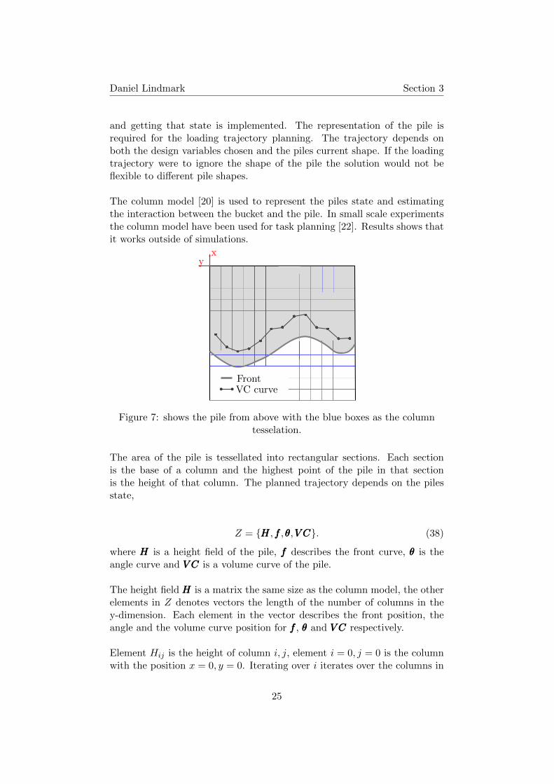
and getting that state is implemented. The representation of the pile isrequired for the loading trajectory planning. The trajectory depends onboth the design variables chosen and the piles current shape. If the loadingtrajectory were to ignore the shape of the pile the solution would not beflexible to different pile shapes.

The column model [20] is used to represent the piles state and estimatingthe interaction between the bucket and the pile. In small scale experimentsthe column model have been used for task planning [22]. Results shows thatit works outside of simulations.

yx

VC curveFront

Figure 7: shows the pile from above with the blue boxes as the columntesselation.

The area of the pile is tessellated into rectangular sections. Each sectionis the base of a column and the highest point of the pile in that sectionis the height of that column. The planned trajectory depends on the pilesstate,

Z = HHH,fff,θθθ,V CV CV C. (38)

where HHH is a height field of the pile, fff describes the front curve, θθθ is theangle curve and V CV CV C is a volume curve of the pile.

The height field HHH is a matrix the same size as the column model, the otherelements in Z denotes vectors the length of the number of columns in they-dimension. Each element in the vector describes the front position, theangle and the volume curve position for fff , θθθ and V CV CV C respectively.

Element Hij is the height of column i, j, element i = 0, j = 0 is the columnwith the position x = 0, y = 0. Iterating over i iterates over the columns in

25


x-dimension and j iterates over y-dimension.

The front fi is defined as the first column in row i equal to zero wheniterating over j = 0, 1, 2, . . . , n.

The angle of a row i is then simply calculated as

θi = tan−1

(Hij

l

)(39)

where l is the length from the front to the volume centrum curve positionand Hij is the height at the volume centrum curve position.

The volume curve position for a row i, is defined as

V Ci =1

VNv

Nv∑j=1

vjxj (40)

where Nv is the number of columns from the front until the point that thesummed volume in the columns equals Vb

(wb/wg) . That is the total volume of

the bucket divided by the number of columns that fit inside the bucket. Thevolume curve position for each row represent this way the volume centrum ofthat row of columns between the front and the column that fills its fractionof the bucket.

3.4 Loading strategy

The controller for the vehicle can be divided into two parts, the planningalgorithm and the execution algorithm. The planner is in charge of planningthe trajectory that the bucket tip should follow. The executer is in charge ofexecuting the planned trajectory and will try to make the bucket tip followthe trajectory as close as possible.

There is an infinite number of trajectories but most of them will be reallybad. A few different categories of trajectories have been proposed [6]. Oneof these is chosen to be investigated. It consists of four stages.

26


A B

C

DE

θ

hd

Figure 8: shows the pile from above with the blue boxes as the columntesselation.

1. A-B, enter the pile with bucket flat on the ground until the planneddepth is reached.

2. B-C, start lifting and tilting the bucket while carving out an equallythick slice from the pile. Until the planned height is reached.

3. C-D, completely tilt the bucket to the maximum tilt angle

4. D-E, and then back away from the pile.

If the planned height in the stage 2 (B-C) are zero the entire stage is skipped,meaning that the bucket will enter the pile and drive into it until the desireddepth is reached then will the executor go directly to stage 3 and just tiltthe bucket back to max. Changing from one stage to another and whatvelocities the actuators of the vehicle should have at any moment is decidedby the execution algorithm. These rules and velocities will of course alsoaffect the production etc. and should ideally be included as design variables,but are excluded in this thesis.

3.4.1 Execution of trajectory

The planned trajectory is executed in the four stages. The executor checksat every time step

• How far the bucket tip has moved in this stage, s.

• How long time spent in this stage.

• What the actual velocities (not the target velocities) of the actuatorsare.

This is then used to set the velocities on the actuators for the next time

27


step and check whether to switch stage or not. The stage can be changedif the maximum time spent in a stage has passed (the vehicle is stuck), ifthe actual velocity of an actuator is less than 10 per cent of the set velocityfor a maximum amount of time (it is too heavy for the vehicle to follow thetrajectory) or if the planned trajectory point is reached. The parameter smeasures how far the bucket tip has moved in the current stage.

s =

√∆x2 + ∆z2 + ∆φ2

x2g + z2

g + φ2g

. (41)

The ∆ terms is how much in that dimension the bucket tip has moved fromthe start of the current stage and the xzφg terms are the goal distances inthat dimension. When s = 1 the goal is met and the executer switches tothe next stage.

vvv(s) =

vx(s)vz(s)wy(s)

(42)

The velocities that the bucket tip should have for following the trajectory aredescribed by the velocity vector in equation (42). The first element is thetranslational velocity in the worlds x-direction, the second is the verticalin the worlds z-direction and the third is the rotation around the worldsy-axis.

Each of the four stages has its own velocity vector defined below by equations(43) to (46).

vvv(s)A-B =

vx000

(43)

vvv(s)B-C =

vx1 (1− s2)vz1(1− s2)wy1(1− s)

(44)

vvv(s)C-D =

00

wy2(1− s2)

(45)

28


vvv(s)D-E =

−vd3(1− s2)00

(46)

In the first stage the bucket tip should only move flat on the ground until itreaches the planned depth, equation (43). Then the bucket is lifted and tilteduntil the bucket tip is at the planned height, equation (44). At that point thebucket is tilted max, equation (45), and then the vehicle is backed up to thestarting position, equation (46). These velocities is then used in equations(35)-(37) for calculating the velocity on the vehicles actuators.

3.4.2 Loading control algorithm

Every time step a new target velocity for the vehicles actuators is calculatedusing the current bucket tip position. The stage is switched to the next oneif the bucket tip have moved into a new stage, s > 1, or if the vehicle is stuck.If the vehicle moved into the fifth stage the loading cycle is completed andat the beginning of the next time step a new trajectory is planned.

Algorithm 1: The algorithm for the loading cycle strategy.

1 while Vehicle running do2 if planNext then3 T ← planTrajectory();4 stage ← 0;5 planNext ← False;

6 end7 s ← calculateS( BuckTipPosition );8 vx, vz, wy ← calculateBucketTipVelocity( s );9 wheelVel, liftVel, tiltVel ← calculateActuatorsVelocity( vx, vz, wy );

10 setActuatorsVelocity(wheelVel, liftVel, tiltVel);11 if s > 1 Or checkStuck() then12 stage ← stage + 113 end14 if stage > 5 then15 planNext ← True;16 end

17 end

29


3.4.3 Planning of trajectory

The planned trajectory, ttt, is a function of the state of the pile, Z, and fourdesign variables,

xxx =[α β γ κ

]T. (47)

By varying the four design variables in equation (47) the structure of theplanned trajectory will change. The planned trajectory can be one that triesto over estimate the filling grade in the bucket or under estimate. It can beone that excavates shallow but high or it can go deep and low etcetera. Thetrajectory is formulated as,

ttt(Z,xxx) =[d h a φ

]T. (48)

where d is the depth, h is the height, a where to attack the pile and φ isthe angle the bucket should tilt during stage 2. ttt then defines the plannedtrajectory in figure 8. The planned height h is calculated using,

h = hmaxβ. (49)

where hmax is the maximum height that the bucket tip can reach on the pilecontour and is calculated using the height field in Z. The design variabel βdecides the fraction of the piles height that the bucket tip aims to end stage2 at. If β = 1 the planned height will be at the maximum height and ifβ = 0 the planned height of stage 2 is zero and the stage is skipped.

The depth controls how much to fill the bucket. Meaning that given a heightthe depth is chosen so that the estimated filling of the bucket is equal to thewanted filling grade αVb. The estimated filling of the bucket is taken to beequal to the volume, V , between the bucket trajectory and the contour ofthe pile. This is the sum of a parallelogram with the base d and the heighth and the circle sector of radius d and angle θ. Setting V = αVb and solvingfor d gives,

d =

(− h

θ+

√h2

θ+

2Vbα

wbθ

). (50)

30


Where wb is the bucket width. With α = 0 the estimated filling grade iszero and the bucket will never enter the pile and with α = 1.0 the estimatedfilling grade will be exactly the volume of the bucket. It is interesting tosee if it is good to over or under estimate the filling grade of the bucket forthe production and damage on equipment. Therefore α is allowed to varybetween the values 0.2 and 2.0.

In stage 2 the bucket will tilt an angle φ. This angle is a fraction of theangle the piles contour makes with the ground.

φ = κθ. (51)

Where θ is the angle of the pile. If κ = 0 the bucket will be held parallelwith the ground during stage 2 but if κ = 1 the bucket will be tilted so thatit at the end of stage 2 is at the same angle as the piles contour.

How to position the vehicle sideways in the tunnel is decided by the designvariable γ and the volume centrum curve defined in equation (40). A lowγ will position the vehicle at a point where the volume centrum is closer tothe back wall while a high γ will position the vehicle at a position that isfurther away from the back wall. The V CV CV C vector is sorted in descendingorder, then is the γ mapped to index the vector. This way γ = 1 will returnthe position that is the furthest away from the back wall and γ = 0 willreturn the position closest to the back wall.

3.5 Objective Function Formulation

The objectives that is investigated in this thesis are the negative productionc1, a measure of damage on the equipment c2, and a measure of the stoppingrate c3. These are all put together into a cost objective function,

CCC(xxx) =

c1(xxx)c2(xxx)c3(xxx)

. (52)

The optimization can be formulated as a minimization problem

31


minimizex

[c1(xxx) c2(xxx) c3(xxx)

]Tsubject to xlow

i ≤ xi ≤ xupperi , i = 1, . . . ,m = Ω.

(53)

Since all of the objectives in CCC will probably compete with each other itwill not exist a single solution where all the objectives are at its optimalvalue. Solving the optimization problem in equation (53) are therefore doneby seeking Pareto-optimal solutions, defined in equation (2).

The production is the mass of material loaded each cycle divided by the timeduration of the loading cycle. Objective c1 is the negative of productionsince the optimization problem is formulated as an minimization problemand production is something you typically want to maximize. The time ismeasured between the beginning of stage 1 and the end of stage 4. Thestages are defined in section 3.4.

c1 = −Mass

Time(54)

The second objective c2 is the damage on the tilt joint, that is joint G infigure 5, but can be applied to all joints. The damage model on that jointbuild on a simple plasticity model. Torques on the joint are observed and ifthe torque is greater than a limit τy an irreversible deformation in the jointis registered. Otherwise is the deformation elastic. The damage is definedas

c2 =1

τy

N∑i=1

max

(τi − τy, 0

)∆t. (55)

Where τi is the magnitude of the torque vector at time step i, τy is a measurehow big the torque can be before the hinge yields and ∆t is the time step.It is only the torque that is included because that it is forces that tries totwist the bucket out of place that is interesting. These kind of torques isarises for example if the bucket is loaded unevenly or driven into a heavyobstacle.

The value of the limit τy should be provided by the manufacturer. In thisthesis τy is decided by testing in the simulation what magnitude the torqueis during a specific situation. In the test the vehicle is placed on a horizontalplane with the bucket flat on the ground. In front of the bucket a static rock

32


is placed. The vehicle is then driven with the maximum velocity into therock and then magnitude of the torque in hinge G is recorded. This is thenset as the threshold τy = 145000 Nm.

The third objective c3 measures the rock spill after a loading trajectory. Therocks that lies in front of the pile are spill rocks and damages the wheelsof the vehicle. When this occurs the loading work may have to paus whileclearing the ground. This is costly because it takes time and affects theoverall production. The measure of how much the rocks in front of the pileaffects the loading work is defined as

c3 =1

Nc

Nc∑i=1

mri

mmax. (56)

After every loading cycle the mass of the rocks in front of the pile are summedtogether and saved as mr =

∑mspill. In equation (56) the mr are scaled

with a maximum mass mmax that is estimated amount of mass that willstop the loading work and then summed over the number of loading cyclesNc.

4 Method

The method for building and exploring the surrogate models of the multi-body dynamic simulations are presented in this section. It starts with sum-marizing the work flow used in this thesis and then defines exactly whatsurrogate model is used. It then finishes with the method for building thesurrogate model.

4.1 Design exploration and optimization

The method proposed in this thesis for performing design exploration andoptimization can be used in other applications than the one discussed inthis thesis. The purpose of it is to make it possible to efficently explorethe design space of an objective function that is the result of an expensivemulti-body dynamic simulation. The simulation is replaced with a surrogatemodel. The steps of the method is summarized below:

33


1. A system model is implemented.

2. An Operation model is implemented.

3. Formulation of the optimization problem.

(a) Define the design variables.

(b) Formulate the objective function.

4. Surrogate model

(a) Generate sample points in the design space using a design ofexperiments (DoE) method.

(b) Perform dynamic simulations using the sample points.

(c) Fit surrogate models to the results from the simulations.

(d) Validate the surrogate models using a independent validation set.

5. Explore the design space using the surrogate models.

6. Design optimization of the design variables using the surrogate models.

Steps 1–3 are application problem specific. The system model in this thesisincludes the vehicle model, tunnel model and granular model. Choosingthe surrogate model is also application problem specific in the sense thatknowledge about the system is required for making an intelligent decision.Since rocks are constantly added in the top of the pile by an emitter usinga mass distribution to generate random rocks the output of the simulationwill be non-deterministic. Noise in all three outputs is expected and thusis the regression Kriging surrogate model chosen. This gives the correlationmatrix on the form

ΨΨΨ =

cor[Y (xxx(1)), Y (xxx(1))] + λ · · · Y (xxx(1)), Y (xxx(n))]...

. . ....

cor[Y (xxx(n)), Y (xxx(1))] · · · Y (xxx(n)), Y (xxx(n))] + λ

, (57)

where

cor[Y (xxx(i)), Y (xxx(l))] = exp

(−

k∑j=1

θj |x(i)j − x

(l)j |

2

). (58)

The basis function used is equation (12) but with the parameters pj =2. The parameters to determine are then the θ:s and the regularization

34


parameter λ. They are found by maximizing the likelihood function inequation (15).

The design exploration is done last when surrogate models that are accurateenough have been obtained. Exploration is done both manually by inspect-ing plots and automatically by running optimization algorithms that findsPareto solutions. With four design variables plotting of the outputs mustbe clever for the explorer to get an understanding of the system. One suchway is a 2D-contour plot in a grid, with two of the design variables varyingover the axes in each plot and the other two variables varying in a discretefashion over the rows and columns in the grid.

4

Example Grid Plot

32

1

c=0

d=0

1 2 3 4 0

5

10

15

Figure 9: Shows f(a, b, c, d) = ac+ 2b2 − 3c on the range [0, 5]

In figure 9 one can see a grid contour plot of the example function f(a, b, c, d) =ac+ 2b2 − 3c, with a and b on the x-/y-axis and c/d vary over the columnsand rows. In the figure one can see that the function is constant in the ddimension.

To find the 3D Pareto front, matlabs gamultiobj function is used with thesurrogate models as objective functions. That is a multi-objective optimiza-tion algorithm using a controlled elitist genetic algorithm [17] and it is basedon the NSGA-II. The obtained Pareto solution can then be plotted as a 3Dscatter plot or as 3 different 2D scatter plot (by projecting the solution down

35


on each of the three planes). From the Pareto plots can the decision makercompare solutions and do trade-off analysis between them.

4.2 SUMO

For building the surrogates the SUMO matlab toolbox is used [8] imple-mented by a research group at Ghent University. The main goal of the tool-box is to build highly accurate global surrogate models for computationalexpensive simulation code. The toolbox provides methods for achieving this,including initial design of experiments (DOE), adaptive sampling algorithmsand many different surrogate model types. The simulation program (hence-forth simulator) interfaces the toolbox. The toolbox is then able to drivethe simulator making it possible to build the surrogates without any userinteraction after the initial configuration of the toolbox.

4.2.1 The control flow

The general control flow of the SUMO toolbox is visualized in figure 10. Itcontinuously adds samples and build new models until it fulfills the criteriaset.

Figure 10: The general SUMO control flow [26].

1. First it generates a set of initial sample points, XXXi.

2. The simulator is called with these sample points. It runs the simula-tions and give back the responses.

36


3. SUMO then generates models while optimizing the model parameters.

(a) The optimization of the model parameters is driven by the mea-sures enabled.

(b) Every time the SUMO build a model with a lower measure scorethe model is saved.

4. When the optimization of the model parameters are done the currentbest models measure score is compared against the criteria set.

5. If the score is not good enough the sequential design generates a newset of sample points and the simulator is called again.

6. Otherwise the best surrogate model is returned.

For every output from the simulation SUMO builds one surrogate model,defined by its own model parameters. This means that step three above willbe repeated for every model that is built and to get the outputs from onesample point xxx all three surrogate models need to be evaluated. Comparedto the simulation where all the outputs are returned at once.

Design Variables Simulation Outputs

Design Variables Surrogate Output

Figure 11: Difference between the simulation and a surrogate model.

4.3 Configuration of SUMO

The SUMO toolbox is configured with two xml files, toolbox configurationand simulator configuration. The toolbox configuration configures the tool-box itself, what model to use, how to score the model, sample strategy, whento finish and so on. In the simulator configuration the interface with thesimulator is defined. That is how many inputs and outputs, ranges, path tothe executable or dataset.

37


Table 4: The toolbox configuration.

Configuration option Value

Initial design LHD with corner points

Sequential design Lola-voronoi ∗ 0.7 + error ∗ 0.3

MeasureName ε τ Use Misc

Validation set RMSE 0.0 Off 20%

Surrogate modelName Basis function Optimizer

Regression Kriging corrGauss fmincon

SUMO

Max number of samples 500

Min number of samples 0

Maximum time Inf

Maximum modeling iterations Inf

LHD with corner points is a Latin Hypercube Design that fill in samplepoints at the corners of the design space. For filling in sample points betweenmodeling iterations a combination of the Lola-Voronoi and the error methodis used. The surrogate model chosen is the regression Kriging. For stoppingthe toolbox a maximum of 500 generated samples are set.

Table 5: The simulator configuration.

Configuration option Value

Design variables

Name Type min,max

α real 0.2,2.0β real 0.0,1.0κ real 0.0,1.0γ real 0.0,1.0

Outputs

Name Type

Production realHingeWear realSpillRock real

ImplementationPlatform Batch Batch Size

Matlab True 8

There are four design variables that control the planning of the loadingtrajectory. The three outputs (responses) defines how many outputs thetoolbox expect to receive from the simulator. For the implementation of thesimulator a matlab script is chosen. Batch is set to true and the batch sizeto eight.

38


4.4 Simulator

The simulator platform is configured as matlab as stated in table 5, butthe actual simulation is implemented as a Lua script interfacing the AgXAPI. An interface between the Matlab script and the Lua script is imple-mented.

Matlab

Python

...Sim1

production.txthingeWear.txtspillRock.txt

SimN

production.txthingeWear.txtspillRock.txt

Figure 12: Shows the structure of the simulator.

The batch mode of the simulator is set to true. This enables SUMO to sendmultiple sample points to the simulator at once and run these simulationsin parallel. The structure of this is shown in figure 12.

1. SUMO calls the specified matlab script with the set of N samplepoints.

2. The matlab script in turn calls a python script with the sample points

3. N simulations are started in parallel by the python script.

4. Every simulation logs the outputs at every time step or loading cycleto a text file.

5. When a simulation is done the python script parses the log files andgives a single scalar value for each output and simulation back tomatlab.

6. Matlab return the outputs back to SUMO

By logging the data in separate text files at a high frequency none of the

39


source data for the output is lost. This makes it possible to investigatedifferent output functions defined in section 3.5 without the need of re-running the simulations. One only needs to rewrite the parser in the Pythonscript and then call that parser with the paths to the data files.

4.4.1 Simulation

The simulations all start from the same initial state. That is the samepile in the same tunnel with the same vehicle. The difference between thesimulations are the design variables that the planned strategy of the vehicledepends on. Thus will every trajectory differ from each other.

In every simulation the vehicle performs one loading cycle on its initial pile,changing the state of the pile. When the pile is at rest again another loadingcycle is planned and executed on the resulting pile. This is repeated 30 timesto reduce noise in the result.

Every simulation will thus have its own tree of resulting piles that the designvariables have created and been tested on. The results will then include theeffect that a certain kind of strategy puts a pile in a state that is hard to loadfrom. The overall production of such a strategy will be lower even thoughit might perform best for one loading cycle.

4.5 AgX

The physics engine AgX Dynamics [1] is used for the simulations. It supportfast simulations of rigid-bodies with non-smooth dynamic, such as contactswith friction. The granular material is represented as rigid bodies withconvex geometry. It is handled with non-smooth discrete element method[24], [19] and an iterative solver.

The vehicle is modelled as constrained rigid bodies. Different actuatorscan be defined by applying a motor on the joints. The vehicle dynamicsis calculated with an direct solver for high precision and stability [12] andthe interaction between the vehicle and environment is handled with a splitsolver. That solves all constraints except for frictional contacts with thedirect solver and then are the normal and frictional contacts solved usingthe iterative solver.

40


5 Results

In this section the surrogate models built from the simulations are presented.First some general results from a simulation then the sample distribution inthe design space is presented, both for the samples used to build the modelsand for validating them. Then the surrogate models are plotted with varyingvalues for the design variables. Continuing with the result for validating saidmodels and finally finishing with the Pareto fronts of the models.

A typical loading cycle was about 12 seconds long. That time can of coursevary a couple of seconds depending on the design variables set. A plannedtrajectory that goes really deep into the pile is typical longer and a shallowtrajectory results in a shorter cycle. One loading cycle took about 15 minutesto simulate. Since one simulation run consisted of 30 cycles the typical timefor one simulation run is about 8 hours including time for the pile to come torest between each cycle. Since 8 simulation ran in parallel all 500 simulationswere completed in about 21 days.

-1 0 1 2 3 4 5 6

Depth [m]

0

0.5

1

1.5

2

2.5

3

Heig

ht [m

]

Pile contour

Planned trajectory

Actual trajectory

(a) The figure shows a goodfollowed trajectory.

-1 0 1 2 3 4 5

Depth [m]

0

0.5

1

1.5

2

2.5

Heig

ht [m

]

Pile contour

Planned trajectory

Actual trajectory

(b) The figure shows a bad followedtrajectory.

Figure 13: The figure shows two planned trajectories and the trajectorythat the bucket actually followed.

The trajectories were followed quite good in some cases but really bad inother. It mostly depends on the type of trajectory. When the plannedtrajectory was low and deep like in figure 13b the execution strategy hada hard time to make the bucket follow the planned trajectory. But if thetrajectory is high and shallow like in figure 13a the trajectory is generallyfollowed a lot better.

In some of the plots below three example points are marked out. They rep-resent three different trajectories that give different responses. The pointsare,

• The red plus: xxx+ =[1.2 0.8 0.8 0.0

],

41


• The red circle: xxx =[0.3 0.6 0.4 0.4

],

• The red cross: xxx× =[1.8 0.1 0.0 0.8

].

The point xxx+ results in a high trajectory (β = 0.8), that over estimates thebucket filling grade with 20 % (α = 1.2), do not tilt the bucket during lifting(κ = 0.0) and positions the vehicle at a point where the front is far away fromthe back wall (γ = 0.8). The trajectory represented by xxx underestimates thebucket filling grade (α = 0.3) and lifts the bucket somewhere in the middle(β = 0.5). The last point xxx× results in a low trajectory that overestimatesthe filling grade of the bucket a lot.

5.1 Sample distribution

The initial design and the sequential design fills the design space with samplepoints. It is important when constructing a global surrogate model to makesure that the design space is filled. Each subplot in figure 14 and 15 showsthe distribution of the samples projected on two axes. So the subplot (2, 1)shows the samples against the design variables α and β. On the diagonal ahistogram of that design variable values is shown.

Sample distribution

0 0.5 1

κ

0 0.5 1

γ

0 0.5 1

β

0 1 2

α

0

0.5

1

κ

0

0.5

1

γ

0

0.5

1

β

0

1

2

α

Figure 14: Shows the distribution of the samples used to build thesurrogate model.

It is clear that the initial design and the sequential design have filled thedesign space well. The sample points are relatively uniformed distributedacross the design space and one can see that the corner points of the design

42


space is represented, thanks to the latin hyper cube with corner points initialdesign. This should be a good set to build the surrogate models with. Thethree example points mentioned above are plotted in figure 14. One cansee that they are spread out around the design space and thus representingdifferent strategies.

Validation set distribution

0 0.5 1

κ

0 0.5 1

γ

0 0.5 1

β

0 1 2

α

0

0.5

1

κ

0

0.5

1

γ

0

0.5

1

β

0

1

2

α

Figure 15: Shows the distribution of the samples used to validate thesurrogate model.

The samples for the validation set were drawn from an uniform randomdistribution.The validation set consists 100 points instead of the 500 pointsused when building the model. The validation sample points is also gener-ated from a completely random process. The design space is filled out nicelyand will be good test to the surrogate model with.

5.2 Surrogate model

The surrogate models were built using the 500 sample points plotted infigure 14. The θ model parameters from this process can be seen in table6. As stated in the theory and from figure 2, a large θ means that thecorresponding design variable is more important. For the production, table6a, α is the design variable that is by far the most important, second mostimportant is β, third κ and fourth γ. For the joint damage β is the mostimportant design variable and α the second most important, κ is still thirdand γ still fourth. For the rock spill surrogate model α is again the mostimportant and β the second most important design variable, κ is howevernot as far behind the other two anymore. γ is still the least important design

43


variable, as it is in all the surrogate models.

Table 6: Tables over the model parameters θj for the production, jointdamage and rock spill surrogate models

(a) Production model parameters

Model parameter Value

θα 0.4332

θβ 0.0466

θγ 0.0020

θκ 0.0058

(b) Joint damage model parame-ters


θα 0.1544

θβ 0.2679

θγ 0.0025

θκ 0.0911

(c) Rock spill model parameters


θα 0.1056

θβ 0.0479

θγ 0.0003

θκ 0.0230

Plotting the resulting surrogate models one can see what the design variablesvalues actually give for output. First is one slice of the models plotted withα and β varying on the x and y-axis respectively and with γ = κ = 0.5 infigures 16 – 18. Then are the surrogate models plotted in nested contourplots in figures 19 – 21, again is the α and β varying on the x and y-axisand within each of the subplots the γ and κ is a constant value.

44


-500

1

-450

-400

-350

0.82

-300

-250

0.61.5

Production

-200

β

-150

α

0.4 1

-100

0.2 0.5

0 0

Figure 16: Shows a slice of the production surrogate model.

The negative production is plotted in figure 16 and one can see that for verylow α (the expected filling grade of the bucket) the production is very lowbut as α increases so does the production. It seems to be the biggest aroundα = 1.0, at least for γ = 0.5 and κ = 0.5 as in this plot.

0

1

5

10

0.8

15

2

20

0.6

25

1.5

Joint damage

β

30

α

0.4 1

35

0.2 0.5

0 0

Figure 17: Shows a slice of the joint damage surrogate model.

The joint damage is clearly the largest around α = 1.0 and then moves downon both sides of that value. This correlates well with the production beingthe highest for that region as well.

45


0.1

1

0.15

0.8

0.2

2

0.25

0.61.5

Rock spill

β

0.3

α

0.4 1

0.35

0.2 0.5

0 0

Figure 18: Shows a slice of the rock spill surrogate model.

If the bucket is overfilled and high above the ground it is likely that morerocks will fall out of the bucket and roll further away from the piles front.This is also seen in the surrogate model in figure 18.

A nested contour plot can show how the model varies with all the designvariables at once. In each figure below the α varies along the x-axis and βalong the y-axis in each subplot, then for each subplot the design variablesκ and γ is held constant. It is then clear that for all the figures 19 - 21 belowthat the surrogate model varies more in the α and β dimension comparedto the κ and γ dimension. This is consistent with θκ and θγ is smaller thanθα and θβ.

46


Figure 19: Shows production surrogate model.

Even though it is small one can see a dependency on the production in theγ and κ dimensions. With γ = 0.8 the maximum production is higher thanwith γ = 0.0. The example point xxx+ results in high production, xxx resultsin low production and xxx× lies in the middle of them.

Figure 20: Shows the joint damage surrogate model.

A clear dependence in the κ dimension can be seen in figure 20. The jointdamage is clearly highest when κ is about in the middle of its range atκ = 0.4. In the γ direction a small dependence is observed. It does notchange the value a lot but the general shape of the contour is changed.Example point xxx+ results in the highest joint damage of the three points,

47


but it is still not the highest joint damage possible in the design space. Thepoint xxx and xxx× both have really low joint damage.

Figure 21: Shows the rock spill surrogate model.

The γ design variable is hardly having any effect on the rock spill surrogatemodel. While a small difference can be seen in the κ direction, mostly thatthe maximum rock spill decreases as κ increases. Example point xxx+ resultsalso in the highest rock spill, xxx results in the lowest rock spill and xxx× againlies in the middle of them.

5.3 Validation of surrogate model

Using the RMSE error function, equation (7), and the validation set the sur-rogate models were validated. The RMSE error function is unit dependentand the value will depend on the range of the function tested, therefore isalso the NRMSE calculated. The validation test shows that the productionsurrogate model is the best at predicting accurate results and that jointdamage and rock spill is about equally good.

Table 7: The RMSE and the NRMSE values for validating the surrogatemodels.

Output RMSE NRMSE

Production 24.81 0.06

Joint damage 6.93 0.16

Rock spill 0.059 0.17

48


5.4 Pareto fronts

For optimizing the problem and finding the optimal set of design variables forall three outputs Pareto fronts are identified using the matlab optimizationfunction gamultiobj.

-550 -500 -450 -400 -350 -300 -250 -200 -150 -100 -50

Production

0

20

40

Join

t dam

age

0.15

0.2

0.25

co

lors

Ro

ck s

pill

-550 -500 -450 -400 -350 -300 -250 -200 -150 -100 -50

Production

0.1

0.2

0.3

Rock s

pill

10

20

30

co

lors

Jo

int

dam

ag

e

0 5 10 15 20 25 30 35

Joint damage

0.1

0.2

0.3

Rock s

pill

-500

-400

-300

-200

-100

co

lors

Pro

ductio

nFigure 22: Shows the three projections and the points are colored after the

value of the final output.

In figure 22 the same Pareto front is plotted in three different subplots. Ineach subplot the points are projected on two of the outputs and the colorsof the points comes from the third output. The example points are alsoplotted for reference. They do however not belong to the Pareto front. Asseen from figures 19-21 the point xxx+ results in high production, rock spilland joint damage. The point xxx results in low production, rock spill andjoint damage. While the point xxx× lies somewhere in the middle.

In the first subplot one can see that the joint damage and production iscompeting in such away that if you want a high production you will need toaccept a high load on the joint. The colors in the subplot shows that at thehigh production and high joint damage the rock spill is high as well. This isalso seen in the middle subplot where rock spill and production are on theaxes. In the last subplot joint damage and rock spill are on the axes showingthe same result with rock spill and joint damage large the production is alsoat it highest.

Unfortunately doing this do not show what the design variables are for eachpoint on the Pareto front. This is instead visualized in the figures 23 - 25below. The Pareto front is again projected on two of the axes but each

49


point on the Pareto front is colored after the value of one of the designvariables.

-550 -500 -450 -400 -350 -300 -250 -200 -150 -100 -50

Production

0

5

10

15

20

25

30

35

Jo

int

da

ma

ge

0.2

0.4

0.6

0.8

1

1.2

1.4

1.6

1.8

2

Th

e c

olo

rs f

rom

α

(a) The colors on the Pareto frontis set from value on α.

-550 -500 -450 -400 -350 -300 -250 -200 -150 -100 -50

Production

0

5

10

15

20

25

30

35

Jo

int

da

ma

ge

0

0.1

0.2

0.3

0.4

0.5

0.6

0.7

0.8

0.9

1

Th

e c

olo

rs f

rom

β

(b) The colors on the Pareto frontis set from value on β.

-550 -500 -450 -400 -350 -300 -250 -200 -150 -100 -50

Production

0

5

10

15

20

25

30

35

Jo

int

da

ma

ge

0

0.1

0.2

0.3

0.4

0.5

0.6

0.7

0.8

0.9

1

Th

e c

olo

rs f

rom

γ

(c) The colors on the Pareto frontis set from value on γ.

-550 -500 -450 -400 -350 -300 -250 -200 -150 -100 -50

Production

0

5

10

15

20

25

30

35

Jo

int

da

ma

ge

0

0.1

0.2

0.3

0.4

0.5

0.6

0.7

0.8

0.9

1

Th

e c

olo

rs f

rom

κ

(d) The colors on the Pareto frontis set from value on κ.

Figure 23: Shows the Pareto front projected on the production and jointdamage axes.

In the figure 23a the points are colored from the design variable α, one cansee that the higher values of α results in higher production and joint damage.One can also see that no α > 1.5 is found. The greatest production comesfrom α ≈ 1.2 and lower production is found for lower α. This is consistentwith the figure 16 and 19.

A high β, figure 23b, generally means high production and joint damage.However are some high β:s also giving a low production and low joint dam-age. This is clearly in combination with really low α values and that cannever lead to high production. The highest production output is clearly aresult of the lowest values κ can have.

50


-550 -500 -450 -400 -350 -300 -250 -200 -150 -100 -50

Production

0.1

0.12

0.14

0.16

0.18

0.2

0.22

0.24

0.26

0.28

0.3

Rock s

pill

0.2

0.4

0.6

0.8

1

1.2

1.4

1.6

1.8

2

Th

e c

olo

rs f

rom

α


-550 -500 -450 -400 -350 -300 -250 -200 -150 -100 -50

Production

0.1

0.12

0.14

0.16

0.18

0.2

0.22

0.24

0.26

0.28

0.3

Rock s

pill

0

0.1

0.2

0.3

0.4

0.5

0.6

0.7

0.8

0.9

1

Th

e c

olo

rs f

rom

β


-550 -500 -450 -400 -350 -300 -250 -200 -150 -100 -50

Production

0.1

0.12

0.14

0.16

0.18

0.2

0.22

0.24

0.26

0.28

0.3

Rock s

pill

0

0.1

0.2

0.3

0.4

0.5

0.6

0.7

0.8

0.9

1

Th

e c

olo

rs f

rom

γ


-550 -500 -450 -400 -350 -300 -250 -200 -150 -100 -50

Production

0.1

0.12

0.14

0.16

0.18

0.2

0.22

0.24

0.26

0.28

0.3

Rock s

pill

0

0.1

0.2

0.3

0.4

0.5

0.6

0.7

0.8

0.9

1

Th

e c

olo

rs f

rom

κ


Figure 24: Shows the Pareto front projected on the production and rockspill axis.

Figure 24 looks a lot like 23 with how the design variables affects the Paretofront. The front is however a lot smoother than the Pareto front in figure23.

51


0 5 10 15 20 25 30 35

Joint damage

0.1

0.12

0.14

0.16

0.18

0.2

0.22

0.24

0.26

0.28

0.3

Rock s

pill

0.2

0.4

0.6

0.8

1

1.2

1.4

1.6

1.8

2

Th

e c

olo

rs f

rom

α


0 5 10 15 20 25 30 35

Joint damage

0.1

0.12

0.14

0.16

0.18

0.2

0.22

0.24

0.26

0.28

0.3

Rock s

pill

0

0.1

0.2

0.3

0.4

0.5

0.6

0.7

0.8

0.9

1

Th

e c

olo

rs f

rom

β


0 5 10 15 20 25 30 35

Joint damage

0.1

0.12

0.14

0.16

0.18

0.2

0.22

0.24

0.26

0.28

0.3

Rock s

pill

0

0.1

0.2

0.3

0.4

0.5

0.6

0.7

0.8

0.9

1

Th

e c

olo

rs f

rom

γ


0 5 10 15 20 25 30 35

Joint damage

0.1

0.12

0.14

0.16

0.18

0.2

0.22

0.24

0.26

0.28

0.3

Rock s

pill

0

0.1

0.2

0.3

0.4

0.5

0.6

0.7

0.8

0.9

1

Th

e c

olo

rs f

rom

κ


Figure 25: Shows the Pareto front projected on the rock spill and jointdamage axis.

When looking at the projection on the rock spill and the joint damage axesin figure 25 it is clear that a low α results in low rock spill and joint damage.The design variable γ effect is the same as α:s, a low value means low rockspill and joint damage, while a high means high joint damage and rockspill.

6 Discussion

In this section the results are discussed. It starts off with looking at how thedesign variables effects the outputs and is it possible to understand why theydo it. Then the optimal set of design variables are discussed. The validationresults are then looked at and what can be done to improve the validationof the surrogate models. The section continues with if the goals have beenfulfilled and finishes with what future work should focus on.

52


6.1 The effect of the design variables.

As seen in table 6, the two most important design variables are α thatcontrols the estimated filling grade of the bucket by adjusting how deep theplanned trajectory will be and β that controls the height of the plannedtrajectory. It is not surprising that these two are the most important sincethey have the most effect on the trajectory shape. The third most importantvariable κ controls how much the bucket is tilted during stage 2 of thestrategy, a low value will keep the bucket parallel with the ground and ahigh will tilt it so the angle with the ground is the same as the contour ofthe pile. It is also expected to have an effect on the three outputs. The tiltingjoint is where the joint damage is investigated and it should be affected byhow the bucket tilts in the path through the granular material. One canalso see that the rock spill is higher with a low κ. Which makes sense sincea low κ means that the bucket is parallel with the ground and it is thuseasier for rock to fall out of the bucket. The least important design variableγ decides where the vehicle is placed during the loading cycle. It appearsthat this have very little effect in all of the models. This could be becausethe difference of the front of the pile is very small and will therefore nevermatter.

A good set of design variables will of course depend on what the decisionmaker is interested in. A high production together with low joint damageand rock spill is probably what you strive for. But since the objectivesare competing the decision maker will have to make a decision what is moreimportant. It could be that the highest measured rock spill in the simulationis acceptable and one can therefore choose a set of design variables that givethe highest production even though it results in high rock spill as well. Orit could be that there is a strict limit the joint damage cannot pass, in thatcase one can look at that limit and find a set of design variables that givesthe highest production possible but is below the joint damage limit.

Taking out a specific set of design variables is therefore not possible withoutmore information about acceptable joint damage and rock spill values. Onecan however say that α should not be higher than 1.2, since higher α thenleads to decreasing production without improving the rock spill and jointdamage response, as seen in figures 23 – 25. Another observation is that thehighest productions is in the higher range of β:s. Even though there is somelow productions as well with high β in figure 24b but this is in combinationwith very low α values and that can never result in high production. Thehighest production values is in combination with high γ values and low κvalues. That is the vehicle is placed so that the bucket will drive into thepile where the front of the pile is far away from the back wall and the bucket

53


do not tilt while being raised.

For keeping the joint damage and rock spill too its minimal the absolutelymost important thing is to choose a small α this is seen in figure 25. Logicalbecause if the bucket is not filled the load on the joint will be small and thenumber of rocks to fall out of the bucket are few.

6.2 The validation of the surrogate model

The production surrogate model is accurate as seen by the validation test.The RMSE is at 6 per cent of the range of the production values in thevalidation data. Given that the buckets total load weight is 21000 kg andthe RMSE is approximately 25 kg/s that is not a big error. The surrogatemodel could be used for predicting the production of different trajectorieswith a good accuracy.

The validation of the joint damage and rock spill is not as satisfying. TheRMSE of 16 and 17 per cent respectively of the range in the validationdata set. The result is still not terrible but these surrogate models are alot worse at predicting results than the production surrogate model. Onecan still rely on the affect the design variables have on the function, but theprediction should be taken with caution. This will also affect the result andthe credibility of the pareto fronts. Meaning that the decision maker cannotrely on the results from these models without improving them first.

Improving the surrogate models could either be done by experimenting withdifferent kinds of basis functions or by changing/improving the functionsmeasuring the joint damage and the rock spill. One could for example lookinto a way of reducing the noise of the models. This could be some kindof filtering function that smooths out the output or completely redefine thefunctions.

6.3 Goals

The goal of the thesis was to produce an effective and robust method forsimulation based exploration of the strategy for a wheel loader and how itaffects the productivity and damage of the machine. This is achieved. Themethod presented in this thesis is capable of exploring the design space ofa strategy for a wheel loader in an effective way. It is shown that the dy-namical simulations can be used to build surrogate models and that those

54


surrogate models are good at predicting the results from the validation sim-ulations. Thus presenting a way of exploring the design space of a strategyand minimizing the number of simulations needed to do so.

6.4 Future work

This thesis have shown it is possible to build surrogate models for the out-put from multi-body dynamical simulations. It is possible to explore thesesurrogate models instead of running individual simulations for each set ofdesign variables one want to test. The simulations have however not beenvalidated against real world data. This must to be done before the surro-gate models can be trusted. That includes fitting of material parameters,validation of vehicle model and kinematics. Right now very little work havebeen put into parameterizing the vehicle correctly. It is essentially put to-gether and given the right weight and strength in the actuators from thespecification, no verification have been done.

The controller developed in this thesis is very simple. It only plans a tra-jectory and sets appropriate velocities on the actuators, it is not particulargood at reacting when getting off track from the planned trajectory and ifthe bucket get stuck the only option is to stop the loading cycle early andback away from the pile. If this method of exploring the design space of astrategy would be used to find an optimal strategy the strategy it self mustbe good before it is going to be worth optimizing it. That includes bothexecution of the strategy, how it handles tough unforeseen situations, as wellas the planning of the strategy. The strategy in this thesis limit it self tothe group of trajectories that carves out an equally thick slice of the pile.Any comparisons on other types of trajectories have not been made.

Adding more design variables is also an option. Everything from the designof the bucket to velocities on the actuators would be interesting. Thenrelastionships between the trajectory shape and the design or the velocitieswould be found.

55

Daniel Lindmark Section A

A Image sequences

A.1 Good loading cycle

(a) (b)

(c) (d)

(e) (f)

(g) (h)

Figure 26: The figures shows a series of images from a loading cycle withhigh production.

A.2 Bad loading cycle

56

Daniel Lindmark Section A

(a) (b)

(c) (d)

(e) (f)

(g) (h)

Figure 27: The figures shows a series of images from a loading cycle withlow production.

57

Daniel Lindmark Section B

B Material Parameters and solver settings

B.1 Material Parameters

The contact materials in the simulations that are used:

Table 8: The rock-bucket contact material

Rolling resistance 0.9

Friction coefficient 1.0

Restitution 0.0

Youngs Modulus 1E8

Table 9: The terrain-bucket contact material



Restitution 0.0

Youngs Modulus 1E8

Table 10: The rock-tire contact material



Restitution 0.0

Youngs Modulus 1E8

58


Table 11: The rock-terrain contact material



Restitution 0.0

Youngs Modulus 1E8

Adhesion* 0

Adhesive Overlap* 0

Table 12: The tire-terrain contact material



Restitution 0.0

Youngs Modulus 1E10

Table 13: The rock-rock contact material



Restitution 0.0

Youngs Modulus 1E10

Adhesion* 0

Adhesive Overlap* 0

* The material property are not set right now.

B.2 Solver settings

The settings that are set on the solver are

• Using parallel PGS: True

• Number of resting iterations: 150

59


References

[1] AgX. AgX-Dynamics User Manual, 2016.

[2] Coetzee, C. J., Basson, A. H., and Vermeer, P. A. Discrete and continuummodelling of excavator bucket filling. Journal of Terramechanics, 44:177–186,2007.

[3] creativecrash. Sandvik loader toro 0011/lh621 3d model, 2016. URLhttps://www.creativecrash.com/3d-model/

sandvik-loader-toro-0011-3d-model.

[4] Dadhich, S. A Survey in Automation of Earth-moving Machines. Technicalreport, Department of Computer Science, Electrical and Space Engineering,Lulea, 2015.

[5] Deb, K., Pratap, A., Agarwal, S., and Meyarivan, T. A Fast and ElitistMultiobjective Genetic Algorithm: NSGA-II. IEEE Transactions onEvolutionary Computation, 6(2), April 2002.

[6] Filla, R., Obermayr, M., and Frank, B. A study to compare trajectorygeneration algorithms for automatic bucket filling in wheel loaders. In Thethird International Commercial Vehicle Techology Symposium, Kaiseralutern,March 2014. doi: 10.13140/RG.2.1.3604.2723.

[7] Forrester, A., Sobester, A., and Keane, A. Engineering design. via Surrogatemodelling. John Wiley & Sons, Inc., New York, 2008.

[8] Gorissen, D., Chouckuyt, I., Dhaene, T., and Demeester, P. A surrogatemodeling and adaptive sampling toolbox for computer based design. Journalof Machine Learning Research, 11:2051–2055, 2010.

[9] Gorissen, D., Chouckuyt, I., Laermans, E., and Dhaene, T. Multiobjectiveglobal surrogate modeling, dealing with the 5-percent problem. Engineeringwith Computers, 26:81–98, 2010. doi: 10.1007/s00366-009-0138-1.

[10] Hemami, A. Motion Trajectory Study in the Scooping Operation of anLHD-Loader. IEEE Transactions on Industry Applications, 30(5):1333–1338,1994.

[11] Hemami, A. and Hassani, F. Simulation Study of a Control Procedure forAutomated Loading of Bulk Media. In The 22nd International Symposiumon Automation and Robotics in Construction (ISARC), Ferrara, September2005.

[12] Lacoursiere, C., Linde, M., and Sabelstrom, O. Direct Sparse Factorization ofBlocked Saddle Point Matrices. In Applied Parallel and Scientific Computing,pages 324–335, Reykjavik, June 2010. 10th International Conference, PARA.

[13] Lacousriere, C. Regularized, stabilized, variational methods for multibodies.In The 48th Scandinavian Conference on Simulation and Modeling (SIMS),pages 40–48. Linkoping University Electronic Press, 2007.

[14] Lacousriere, C., Servin, M., and Backman, A. Fast and stable simulation ofgranular matter and machines. In Discrete element methods - Simulation ofDiscontinua: Theory and applications, London, August 2010. The FifthInternational Conference on Discrete Element Methods.

60


[15] LKAB. Sub-level caving lkab, 2016. URL https:

//www.lkab.com/en/About-us/Overview/Mining/Sub-Level-Mining/.

[16] Marshall, J., Murphy, P., and Daneshmend, L. Toward AutononmousExcavation of Fragmented Rock: Full-Scale Experiments. IEEE Transactionson Automatic Science and Engineering, 5(3), July 2008.

[17] Matlab. Controlled elitist genetic algorithm, 2016. URL http:

//se.mathworks.com/help/gads/gamultiobj.html?requestedDomain=

www.mathworks.com&requestedDomain=se.mathworks.com.

[18] Obayashi, S., Jeong, S., and Chiba, K. Multi-Objective Design Explorationfor Aerodynamic Configurations. In 35th AIAA Fluid Dynamics Conferenceand Exhibit, Toronto, June 2005.

[19] Radjai, F. and Dubois, F. Discrete-element Modeling of Granular Materials.ISTE Ltd and John Wiley & Sons, Inc, New York, 2011.

[20] Sarata, S. Model-based task planning for loading operation in mining. InIntelligent Robots and Systems, volume 1, pages 439–445, Maui, 2001.

[21] Sarata, S., Osumi, H., Kawai, Y., and Tomita, F. Trajectory arrangement ofbucket motion of wheel loader. In IEEE International Conference onRobotics and Automation, pages 3488–3493, New Orleans, April 2005.

[22] Sarata, S., Weeramhaeng, Y., and Tsubouchi, T. Approach Path Generationto Scooping Position for Wheel Loader. In IEEE International Conference onRobotics and Automation, pages 1809–1814, Barcelona, April 2005.

[23] Servin, M. and Wang, D. Adaptive model reduction for nonsmooth discreteelement simulation. Computational Particle Mechanics, 3:107–121, 2016. doi:10.1007/s40571-015-0100-5.

[24] Servin, M., Wang, D., Lacoursiere, C., and Bodin, K. Examining the smoothand nonsmooth discrete element approaches to granular matter. InternationalJournal for Numerical Methods in Engineering, 97(12):878–902, 2014.

[25] Spong, M. W., Hutchinson, S., and Vidyasagar, M. Robot Modeling andControl. John Wiley & Sons, Inc., New York, 2006. ISBN 0-47164990-2.

[26] SUMO. Sumo wiki page, 2016. URLhttp://sumowiki.intec.ugent.be/Main_Page.

[27] Vapnik, V. Statistical Learning Theory. John Wiley & Sons, Inc., New York,1998.

[28] Wang, G. G. and Shan, S. Review of metamodeling techniques for productdesign with computational intensive processes. Journal of MechanicalDesign, 129(4), 2007.

[29] Wimmer, M., Nordqvist, A., Righetti, E., Petropoulos, N., and Thurley,M. J. Analysis of Rock Fragmentation and its Effect on Gravity Flow at theKiruna Sublevel Caving Mine. In 11th International Symposium on RockFragmentation by Blasting : FragBlast11, pages 891–921, Sydney, August2015.

61

simulation based exploration of a loading strategy...

Documents