simulating corporate income tax reform proposals … · simulating corporate income tax reform...
TRANSCRIPT
Simulating Corporate Income Tax Reform Proposals
With a DCGE Model
K. Bhattarai1, J. Haughton2, M. Head3 and D.G. Tuerck4
September 2015
Abstract
U.S. opinion leaders and policy makers have turned their focus to the corporate income tax, which is now the highest in the developed world. Using a dynamic computable general equilibrium model (the “NCPA-DCGE Model”), we simulate alternative policies for reducing the U.S. corporate income tax. We find that all hypothesized policies result in significant positive impacts on output, investment, capital formation, employment and household well-being. All of the hypothesized reforms also result in a more streamlined public sector. These results are plausible insofar as the DCGE model from which they were obtained is parameterized by plausible elasticity assumptions and incorporates the adjustments in prices, output, employment and investment that result from changes in tax policy.
Research for this paper was conducted under a grant from the National Center for Policy Analysis, 14180 Dallas Parkway, Suite 350, Dallas, Texas 75254 1Keshab Bhatterai. The Business School, University of Hull, Cottingham Road, Hull, HU6 7SH, UK; [email protected], phone: 44-1482463207; fax: 44-1482463484; Web: http://www.hull.ac.uk/php/ecskrb/. 2Jonathan Haughton. Department of Economics and Beacon Hill Institute at Suffolk University, 8 Ashburton Place, Boston, MA 02108; [email protected], phone: 617-573-8750 fax: 617-994-4279; Web: http://web.cas.suffolk.edu/faculty/jhaughton/. 3 Michael Head, Department of Economics and Beacon Hill Institute at Suffolk University, 8 Ashburton Place, Boston, MA 02108; [email protected] 617-573-8750 fax: 617-994-4279; Web: www.beaconhill.org. 4 David G. Tuerck. Department of Economics and Beacon Hill Institute at Suffolk University, 8 Ashburton Place, Boston, MA 02108; [email protected], phone: 617-573-8263; fax: 617-994-4279; Web: www.beaconhill.org.
2
Table of Contents
1. Introduction .................................................................................................................................. 3
2. The Formal Specification of the DCGE Model of the US Economy ........................................... 9
2.1 Main Features of the Model ................................................................................... 9
2.2 Preferences ........................................................................................................... 10
2.3 Production Function ............................................................................................. 13
2.4 Labor Supply and Capital Accumulation ............................................................ 16
2.5 Foreign Direct Investment and Capital Inflows ................................................... 18
2.6 Calibration............................................................................................................ 19
3. The Current Tax System and Elasticities ..................................................................................... 21
4. Results of the DCGE with Corporate Tax Reforms ..................................................................... 25
5. Macro Impacts of Alternative Corporate Income Tax Rates ....................................................... 37
6. Conclusion ................................................................................................................................... 38
7. References .................................................................................................................................... 39
8. Glossary for Sectors ..................................................................................................................... 40

3
1. Introduction
U.S. corporate tax reform has emerged as a dominant issue in the political season now upon
American voters. Tax reform proposals have been put forward by President Barack Obama
and several candidates for president.1 The political campaign for president offers an
opportunity to revisit the rich academic literature, which seeks to explain the burden
corporate taxes places on investment. This paper aims to provide information useful to both
the political debate and to the academic literature.
The debate over corporate taxes ties into the broader debate over how best to satisfy the two
major goals of sound tax policy: efficiency and equity. The tension between the two
objectives is inseparable from policy debates, but there is a growing consensus that the
existing U.S. tax system is highly inefficient. Mirrlees et al. (2010), writing about the United
Kingdom, speaks of a hopeful consensus among most economists observing that "there are
taxes that are fairer, less damaging, and simpler than those that we have now. To implement
them will take a government ...willing to put long term strategy ahead of short term tactics."
As early as 1985, Hall and Rabushka (2007) in the U.S. expressed the urgency for tax reform,
by declaring “it is time for another Declaration of Independence, this time from an unfair,
costly, complicated federal income tax. The alternative is a low simple flat tax.”
The purpose of this paper is to assess the effects of corporate tax reform on the U.S.
economy. This analysis is the first based on the dynamic computable general equilibrium
model we are building for the National Center for Policy Analysis – Dynamic Computable
General Equilibrium (NCPA-DCGE). The purpose of the NCPA-DCGE Model is to examine
U.S. tax policy changes for their effects on major economic indicators, including:
• The level and distribution of household income; • GDP, capital investment, and private sector employment; • Government tax revenues, employment and spending; and, • Short-term and long-term consumer welfare.
1 For a review of several corporate tax reforms under consideration see James P. Angelini and David G. Tuerck, “The U.S. Corporate Income Tax: A Primer for U.S. Policymakers,” The Beacon Hill Institute at Suffolk University and the National Center for Policy Analysis (July 2015), http://www.ncpa.org/pdfs/sp_The%20U.S.%20Corporate%20Income%20Tax.pdf.
4
Dynamic CGE models are the most appropriate tools for assessing the impacts of taxes. Our
earlier study found significant benefits from the implementation of the FairTax in terms
growth and redistribution in the US economy (Bhattarai, Haughton and Tuerck, forthcoming
2015). This paper focuses on the impacts of changes in corporate income taxes, and the
model uses the micro-consistent data from a Social Accounting Matrix (SAM2015) for
benchmarking.
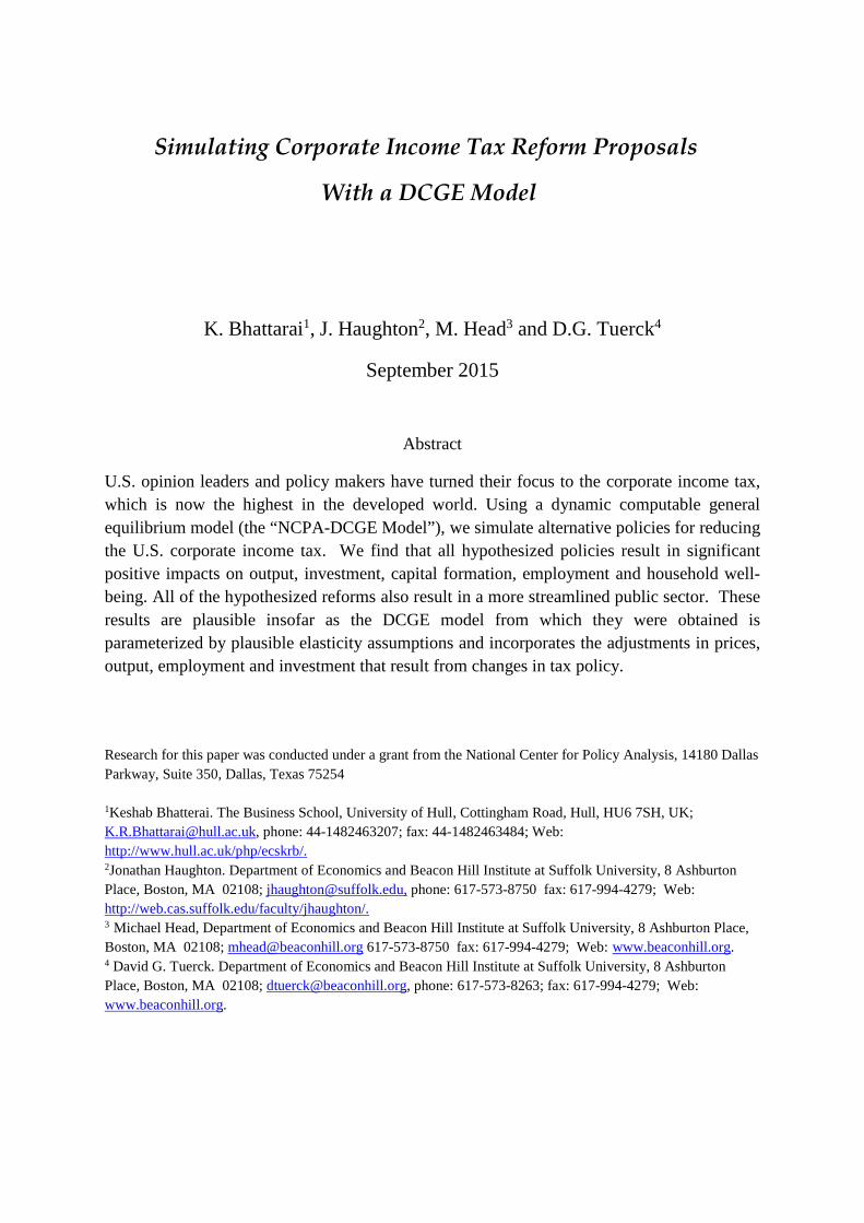
There are three main reasons why we focus on corporate tax reform here. First, as shown in
Figure 1.1, the United States has the highest statutory tax rate among OECD countries. In their
survey of the literature, Angelini and Tuerck (2015) find U.S. corporate rates to be relatively
high and to impose a substantial burden on the U.S. economy. While several other countries,
including Japan, Germany and the UK, have reduced corporate taxes substantially, the United
States still has a combined federal, state and local corporate tax rate of greater than 39 percent.
Overesch and Rincke (2011) provide an analysis of the declining rate of corporate taxes
across the OECD economies. Leibrecht and Hochgatterer (2012) and Zellner, Ngoie and
Kibambe (2015), attribute these falling rates of corporate taxes in OECD countries to the
pace of globalization and tax competition.
Second, the high U.S. corporate tax rate appears to represent an inefficient source of revenue.
Despite a lower average tax rate (ATR), the marginal tax rate is quite high in the corporate
income in the US. This creates distortions. As shown in Figure 1.2, U.S. corporate tax
revenue has represented only two percent of GDP in recent years, and is small in comparison
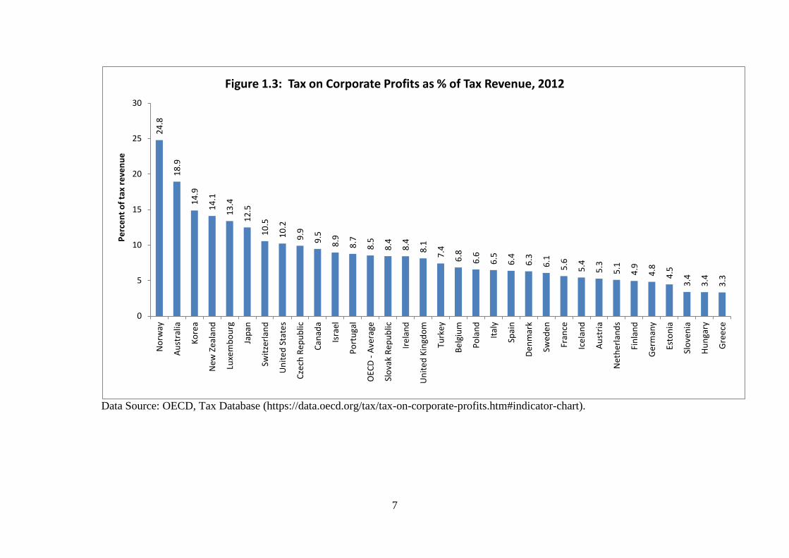
to the average of the OECD economies. The U.S. corporate tax contributed about 10 percent
of total tax revenue, compared to 8.5 percent across OECD countries. Finally, and as we show
below, the existing corporate tax rate imposes a substantial burden on the U.S. economy.
Third, tax reform is back on the political agenda, and features prominently in the policy
platforms of several of the leading candidates for the presidency.
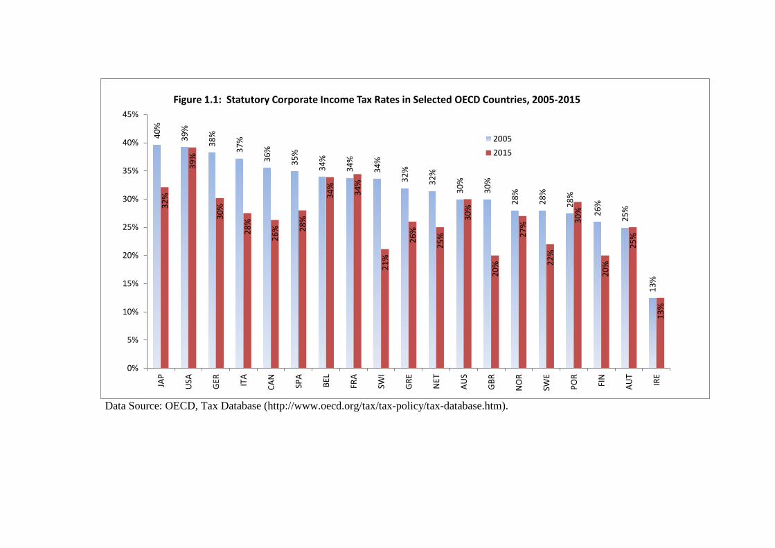
Data Source: OECD, Tax Database (http://www.oecd.org/tax/tax-policy/tax-database.htm).
40%
39%
38%
37%
36%
35%
34%
34%
34%
32%
32%
30%
30%
28%
28%
28%
26%
25%
13%
32%
39%
30%
28%
26% 28
%
34%
34%
21%
26%
25%
30%
20%
27%
22%
30%
20%
25%
13%
0%
5%
10%
15%
20%
25%
30%
35%
40%
45%
JAP
USA GER IT
A
CAN
SPA
BEL
FRA
SWI
GRE NET
AUS
GBR
NO
R
SWE
POR
FIN
AUT
IRE
Figure 1.1: Statutory Corporate Income Tax Rates in Selected OECD Countries, 2005-2015
20052015

6
Data Source: OECD, Tax Database (http://www.oecd.org/tax/tax-policy/tax-database.htm).
0
0.5
1
1.5
2
2.5
3
3.5
4
4.5
5
1965
1970
1975
1980
1985
1990
1995
2000
2005
2010
perc
ent
Figure 1.2: Ratio Corporate Tax Revenue to GDP for US, UK and OECD, 1965-2013
UK
USA
OECD
7
Data Source: OECD, Tax Database (https://data.oecd.org/tax/tax-on-corporate-profits.htm#indicator-chart).
24.8
18.9
14.9
14.1
13.4
12.5
10.5
10.2
9.9
9.5
8.9
8.7
8.5
8.4
8.4
8.1
7.4
6.8
6.6
6.5
6.4
6.3
6.1
5.6
5.4
5.3
5.1
4.9
4.8
4.5
3.4
3.4
3.3
0
5
10
15
20
25
30
Nor
way
Aust
ralia
Kore
a
New
Zea
land
Luxe
mbo
urg
Japa
n
Switz
erla
nd
Uni
ted
Stat
es
Czec
h Re
publ
ic
Cana
da
Isra
el
Port
ugal
OEC
D - A
vera
ge
Slov
ak R
epub
lic
Irela
nd
Uni
ted
King
dom
Turk
ey
Belg
ium
Pola
nd
Italy
Spai
n
Denm
ark
Swed
en
Fran
ce
Icel
and
Aust
ria
Net
herla
nds
Finl
and
Ger
man
y
Esto
nia
Slov
enia
Hung
ary
Gre
ece
Perc
ent o
f tax
reve
nue
Figure 1.3: Tax on Corporate Profits as % of Tax Revenue, 2012
8
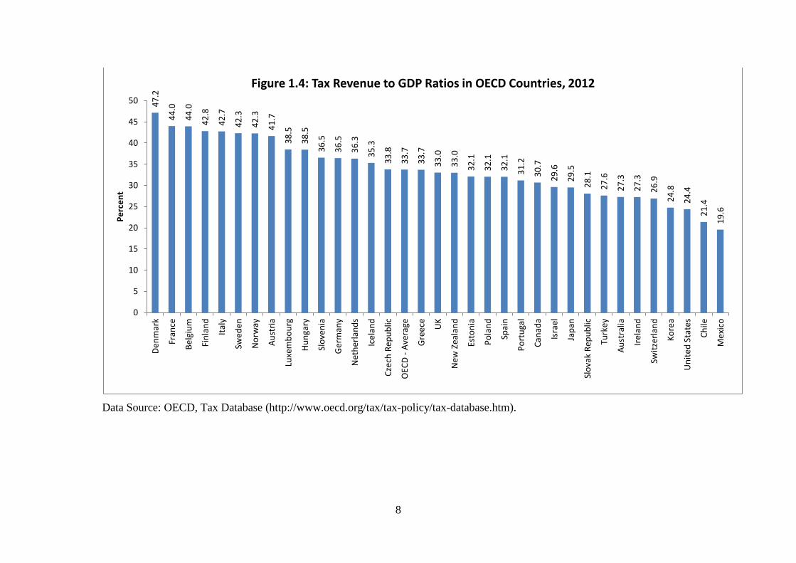
Data Source: OECD, Tax Database (http://www.oecd.org/tax/tax-policy/tax-database.htm).
47.2
44.0
44.0
42.8
42.7
42.3
42.3
41.7
38.5
38.5
36.5
36.5
36.3
35.3
33.8
33.7
33.7
33.0
33.0
32.1
32.1
32.1
31.2
30.7
29.6
29.5
28.1
27.6
27.3
27.3
26.9
24.8
24.4
21.4
19.6
0
5
10
15
20
25
30
35
40
45
50
Denm
ark
Fran
ce
Belg
ium
Finl
and
Italy
Swed
en
Nor
way
Aust
ria
Luxe
mbo
urg
Hung
ary
Slov
enia
Ger
man
y
Net
herla
nds
Icel
and
Czec
h Re
publ
ic
OEC
D - A
vera
ge
Gre
ece
UK
New
Zea
land
Esto
nia
Pola
nd
Spai
n
Port
ugal
Cana
da
Isra
el
Japa
n
Slov
ak R
epub
lic
Turk
ey
Aust
ralia
Irela
nd
Switz
erla
nd
Kore
a
Uni
ted
Stat
es
Chile
Mex
ico
Perc
ent
Figure 1.4: Tax Revenue to GDP Ratios in OECD Countries, 2012

9
2. The Formal Specification of the DCGE Model of the US Economy
2.1 Main Features of the Model There is an extensive literature that identifies the excess burden of corporate taxes on
investment. Angelini and Tuerck (2015) show how corporate taxation in the U.S. imposes a
double tax on investors. But past studies are mostly comparative static, partial equilibrium
analyses.
A general equilibrium model is a complete specification of the price system in which
quantities and prices are determined by the interaction of the demand and supply of goods
and factor markets. Governments influence market outcomes by altering prices by means of
taxes and transfers and, in the process, exert significant impacts on investments and the
economic growth rate of various sectors of the economy. The NCPA-DCGE model allows for
labor-leisure choices, and consumption-saving choices, both in the current period and over
time. The household is assumed to adopt an optimization rule, which it revises in response to
tax-policy changes.
In the NCPA-DCGE model, the structural features of the U.S. economy are akin to those
adopted in Bhattarai, Haughton and Tuerck (2015). The model can be used to compare
alternative tax policies to determine which are more efficient in terms of maximizing the
welfare of U.S. households, consistent with existing levels of technology, and labor and
capital endowments.
Households and producers optimize, given their budget and time constraints. Price
adjustments bring about the most efficient economic outcomes. The general equilibrium is
achieved when excess demand is zero in each market for each period, representing balance
between demand and supply. The existence of the general equilibrium is guaranteed by fixed
point theorems, and the model is solved using the dynamic routines in the GAMS/MPSGE
software.2 Given the desirable properties of the Constant Elasticity of Substitution (CES) or
2 General Algebraic Modeling Systems. http://www.gams.com/ and Mathematical Programming System for General Equilibrium Analysis. http://www.gams.com/solvers/mpsge/.
10
Cobb-Douglas demand and supply functions, equilibrium is stable and unique, and will
determine the evolution of the model economies from 2017 to 2050.
The next sections describe the components of the model in more detail.
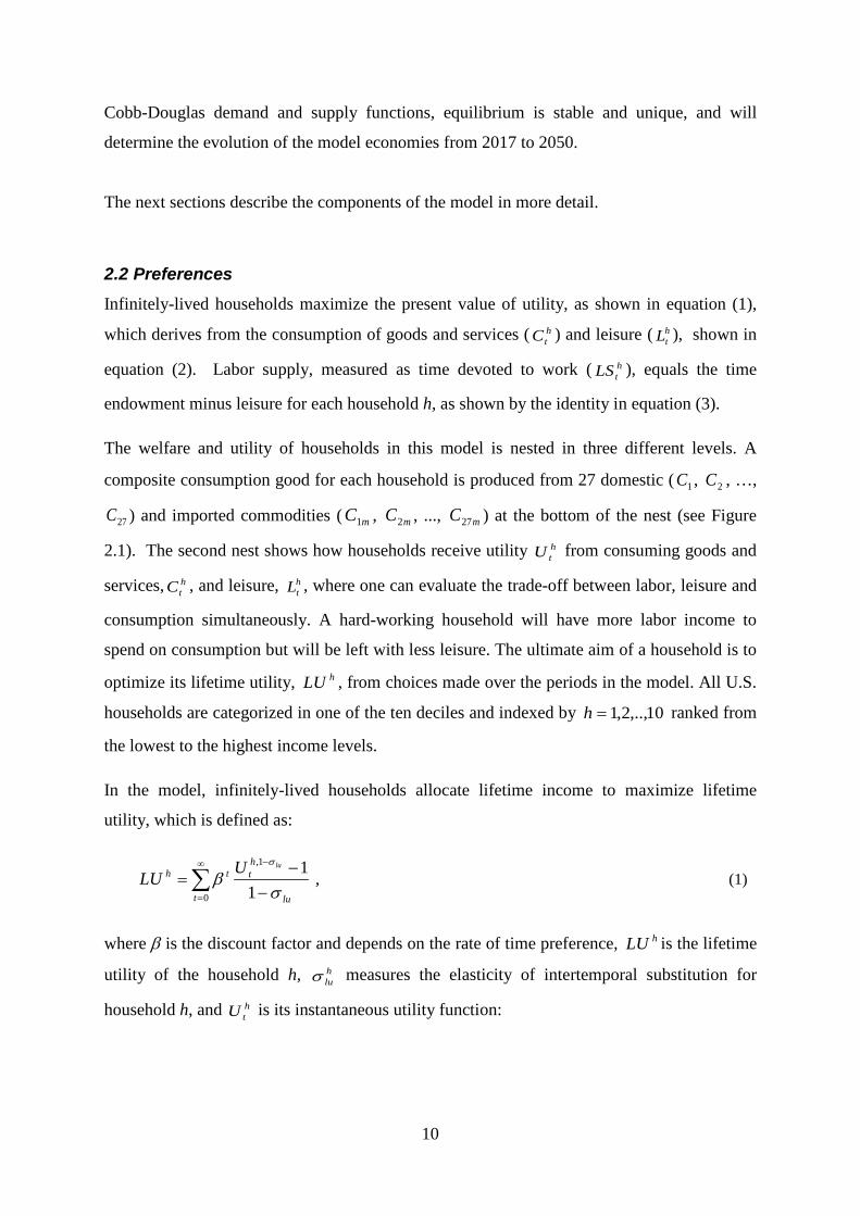
2.2 Preferences Infinitely-lived households maximize the present value of utility, as shown in equation (1),
which derives from the consumption of goods and services ( htC ) and leisure ( h
tL ), shown in
equation (2). Labor supply, measured as time devoted to work ( htLS ), equals the time
endowment minus leisure for each household h, as shown by the identity in equation (3).
The welfare and utility of households in this model is nested in three different levels. A
composite consumption good for each household is produced from 27 domestic ( 1C , 2C , …,
27C ) and imported commodities ( mC1 , mC2 , ..., mC27 ) at the bottom of the nest (see Figure
2.1). The second nest shows how households receive utility htU from consuming goods and
services, htC , and leisure, h
tL , where one can evaluate the trade-off between labor, leisure and
consumption simultaneously. A hard-working household will have more labor income to
spend on consumption but will be left with less leisure. The ultimate aim of a household is to
optimize its lifetime utility, hLU , from choices made over the periods in the model. All U.S.
households are categorized in one of the ten deciles and indexed by 10,..,2,1=h ranked from
the lowest to the highest income levels.
In the model, infinitely-lived households allocate lifetime income to maximize lifetime
utility, which is defined as:
∑∞
=
−
−−
=0
1,
11
t lu
htth
luULU
σβ
σ
, (1)
where β is the discount factor and depends on the rate of time preference, hLU is the lifetime
utility of the household h, hluσ measures the elasticity of intertemporal substitution for
household h, and htU is its instantaneous utility function:
11
111
)1(),(
−
−+=
−− hu
hu
hu
hu
hu
hu
ht
hc
ht
hc
ht
ht LCLCU
σ
σ
σ
σ
σ
σ
αα . (2)
ht
ht
ht LLLS −= . (3)
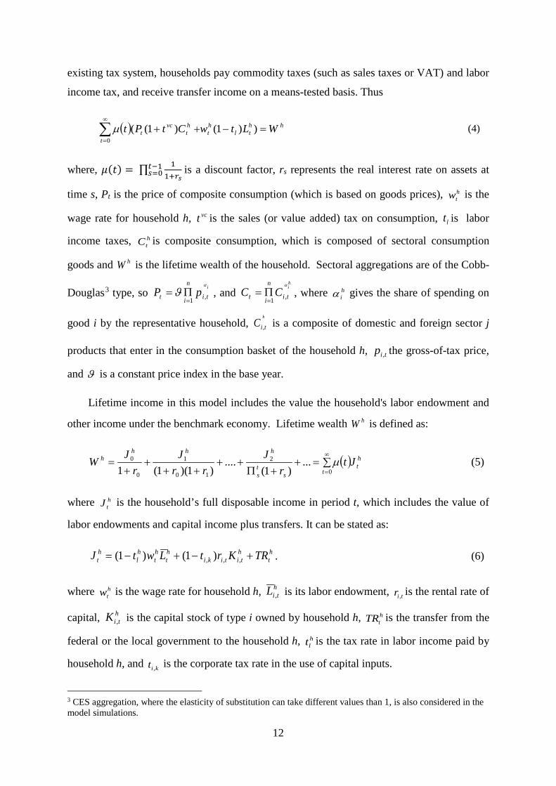
Figure 2.1 Nesting of Utilities
C1 C2 C3 C4 C5 C6 C7 C8 C9 C10 C11 C12 C13 C14 C15 C16 C17 C18 C19 C 20 C21 C22 C23 C24 C25 C26 c27
C1m C2m C3m C4m C5m C6m C7m … ….…….C14m C15m C16m C17m C18m C19m C20m …… …………………….…. C25 C26m c27m
Lifetime and Instantaneous Utility Function of a Household in the NCPA-DCGE Model
huσ
hcσ
htU
htLh
tC
hLU
hU1hU 2
hTU
hluσ
Here htC is composite consumption in period t, and h
tL is leisure in period t, hcα is the
consumption share of household h, and hcσ and h
uσ respectively represent elasticities of
substitution between goods and services and between consumption and leisure. The larger the
value of huσ , the more responsive are consumption and labor supply to changes in commodity
prices and wage rates.
The representative household in each income decile faces an intertemporal budget
constraint whereby the present value of its consumption and leisure in all periods cannot
exceed the present value of infinite lifetime full income (wealth constraint), hW . In the
12
existing tax system, households pay commodity taxes (such as sales taxes or VAT) and labor
income tax, and receive transfer income on a means-tested basis. Thus
( ) hhtl
ht
t
ht
vct WLtwCtPt =−++∑
∞
=
))1()1((0µ (4)
where, 𝜇𝜇(𝑡𝑡) = ∏ 11+𝑟𝑟𝑠𝑠
𝑡𝑡−1𝑠𝑠=0 is a discount factor, rs represents the real interest rate on assets at
time s, Pt is the price of composite consumption (which is based on goods prices), htw is the
wage rate for household h, vct is the sales (or value added) tax on consumption, lt is labor
income taxes, htC is composite consumption, which is composed of sectoral consumption
goods and hW is the lifetime wealth of the household. Sectoral aggregations are of the Cobb-
Douglas3 type, so i
ti
n
it pPα
ϑ ,1=Π= , and
hi
ti
n
it CCα
,1=Π= , where h
iα gives the share of spending on
good i by the representative household, h
tiC , is a composite of domestic and foreign sector j
products that enter in the consumption basket of the household h, tip , the gross-of-tax price,
and ϑ is a constant price index in the base year.
Lifetime income in this model includes the value the household's labor endowment and
other income under the benchmark economy. Lifetime wealth hW is defined as:
( ) ht
tsts
hhhh Jt
rJ
rrJ
rJ
W ∑=++Π
++++
++
=∞
=0
2
10
1
0
0 ...)1(
....)1)(1(1
µ (5)
where htJ is the household’s full disposable income in period t, which includes the value of
labor endowments and capital income plus transfers. It can be stated as:
ht
htitiki
ht
ht
hl
ht TRKrtLwtJ +−+−= ,,, )1()1( . (6)
where htw is the wage rate for household h, h
tiL , is its labor endowment, tir , is the rental rate of
capital, htiK , is the capital stock of type i owned by household h, h
tTR is the transfer from the
federal or the local government to the household h, hlt is the tax rate in labor income paid by
household h, and kit , is the corporate tax rate in the use of capital inputs.
3 CES aggregation, where the elasticity of substitution can take different values than 1, is also considered in the model simulations.
13
We combine equations (1) to (6) to form the Lagrangian for the consumer’s intertemporal
allocation problem in (7):
( ) ]))1()1(,)1(([1
1)1(
)1
1(0
1
1,
0
11
hhtk
ht
htl
ht
ht
vc
tt
hhu
ht
hc
ht
hc
t
t
h WKtrkLtwCtPt
LC
hu
hu
hu
hu
hu
hu
hu
−−+−+++−
−
−+
+=ℑ ∑∑
∞
=
−
−
∞
=
−−
µλσ
αα
ρ
σ
σ
σ
σ
σ
σ
σ
.
(7)
Here, huσ is the intratemporal elasticity of substitution between consumption and leisure, h
cα
is the consumption share of household h, hλ is the shadow price of income in terms of the
present value of utility, and β is replaced byρ+1
1 , where 0>ρ is the rate of time preference,
which indicates the degree to which the household prefers leisure and consumption in earlier
rather than in later years.
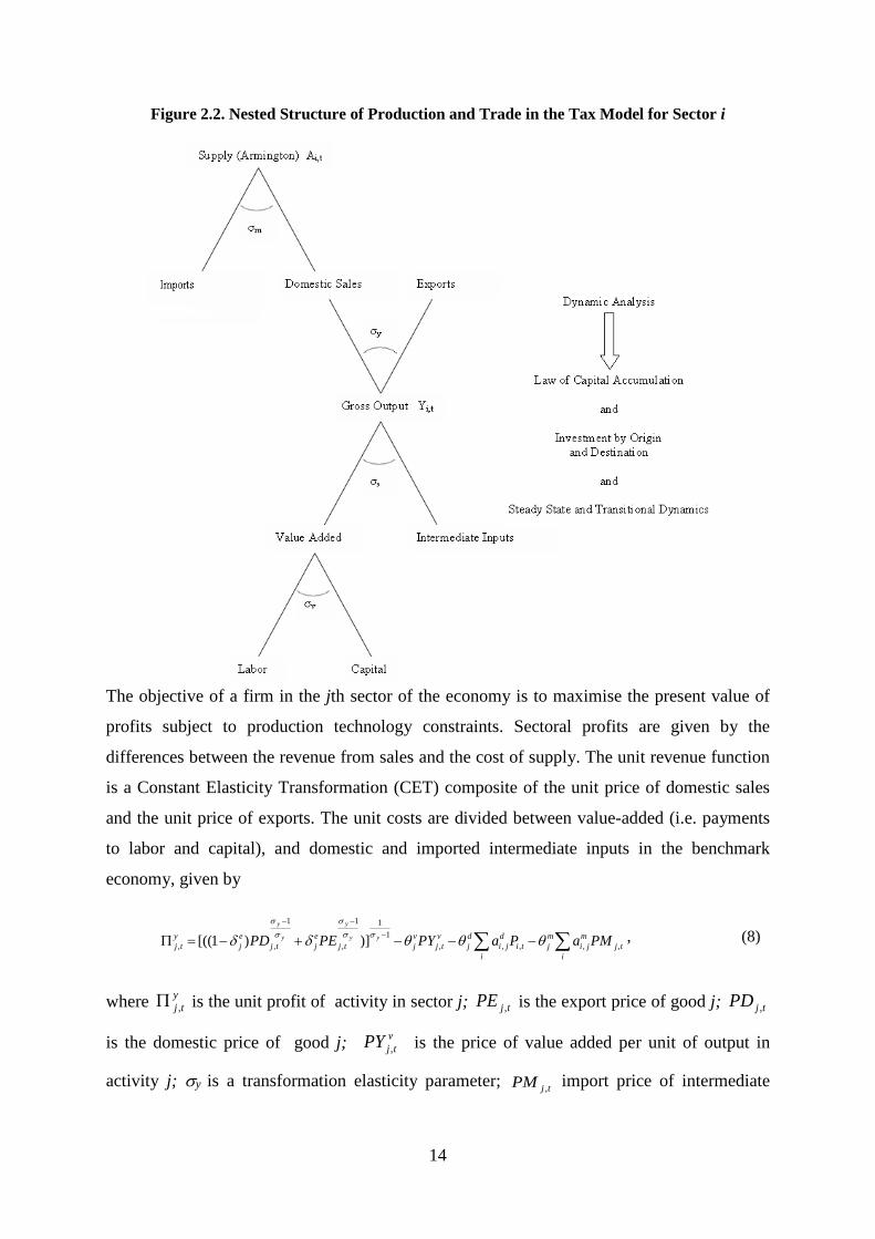
2.3 Production Function
In each period, the supply process in this economy can be explained by nested production
functions for each of 27 sectors. Producers use intermediate inputs in fixed proportions (a
“Leontief” technology), but there is flexibility in the use of capital and labor. The nested
production structure in Figure 2.2 includes a composite labor supply function from ten
categories of households; a sector-specific capital accumulation and capital allocation
function; a value-added function; a Leontief function between value added and intermediate
inputs; a constant elasticity of transformation (CET) export function between U.S. markets
and the rest of the world; a constant elasticity of substitution (CES) function between
domestically supplied goods and imports; and a measure of total absorption in the economy.
14
Figure 2.2. Nested Structure of Production and Trade in the Tax Model for Sector i
The objective of a firm in the jth sector of the economy is to maximise the present value of
profits subject to production technology constraints. Sectoral profits are given by the
differences between the revenue from sales and the cost of supply. The unit revenue function
is a Constant Elasticity Transformation (CET) composite of the unit price of domestic sales
and the unit price of exports. The unit costs are divided between value-added (i.e. payments
to labor and capital), and domestic and imported intermediate inputs in the benchmark
economy, given by
∑∑ −−−+−=Π −
−−
itj
mji
mj
iti
dji
dj
vtj
vjtj
ejtj
ej
ytj PMaPaPYPEPD yy
y
y
y
,,,,,1
11
,
1
,, )])1[(( θθθδδ σσσ
σσ
, (8)
where ytj ,Π is the unit profit of activity in sector j; tjPE , is the export price of good j; tjPD ,
is the domestic price of good j; vtjPY , is the price of value added per unit of output in
activity j; σy is a transformation elasticity parameter; tjPM , import price of intermediate
15
input; Pi t, is the price of final goods used as intermediate goods; ejδ is the share parameter
for exports in total production; vjθ is the share of costs paid to labor and capital; d
jθ is the
cost share of domestic intermediate inputs; mjθ is the cost share of imported intermediate
inputs; the djia , are input-output coefficients for domestic supply of intermediate goods; and
the mjia , are input-output coefficients for imported supply of intermediate goods.
Producers maximize the net of tax profit ( ytjF ,Π ) as:
( )
−−−+−−=Π ∑∑−
−−
itj
mji
mj
iti
dji
dj
vtj
vjtj
ejtj
eji
ytj PMaPaPYPEPDtF yy
y
y
y
,,,,,1
11
,
1
,, )])1[((1 θθθδδ σσ
σ
σ
σ
(9)
The government takes a part of pre-tax profit as its revenue from taxes on profits ( FR ) as:
−−−+−=Π= ∑∑−
−−
itj
mji
mj
iti
dji
dj
vtj
vjtj
ejtj
eji
ytjiF PMaPaPYPEPDttR yy
y
y
y
,,,,,1
11
,
1
,, )])1[(( θθθδδ σσ
σ
σ
σ
(10)
At the bottom of the nest of the production side of the economy, producers use labor and
capital in each of N sectors to produce value added. The amount of each type of these inputs
employed by a producer in a particular sector is based upon the sector-specific production
technology and input prices. We use a CES function to express this relationship:
( ) vvv
tiitiii LSKtiY σσ
δδ σ1
,, )())(1(, +−Ω= , (11)
where tiY , is the gross value added of sector i, iΩ is a shift or scale parameter in the
production function, tiK , and tiLS , are the amounts of capital and labor used in sector i, iδ is
the share parameter of labor in production, and vσ is the CES substitution elasticity
parameter. This is a constant-returns-to-scale production function. Euler's product exhaustion
theorem implies that total output (value added) equals payments to labor and capital, and
each factor receives remuneration at the rate of its marginal productivity:
tititittiti KrkLSwYPY ,,,,, += (12)

16
where tw is the gross-of-tax composite wage rate that the employer pays to use labor input,
and tirk , is the gross rental rate of capital. Note that the tw is a composite of wage rates for
each category of household, htw ; similarly, tiLS , is the composite of h
tiLS , , the labor supplied
by households, for h =1, 2,…, 10.
Then the second nest in production is given by the relationship between the intermediate
inputs and gross output as expressed by input-output coefficients, which form a fixed
physical non-price based constraint on the production system. The general form of the
production function is
=
== jim
ji
tji
jid
ji
tjititi a
MIa
DIYGY
,
,,
,
,,,, ,,min (13)
where the djia , are input-output coefficients for domestic supply of intermediate goods; m
jia ,
are input-output coefficients for imported supply of intermediate goods, tjiDI ,, is the supply
of domestic intermediate input and tjiMI ,, is the supply of imported intermediate inputs. The
presence of input-output linkages in the model enables us to assess various kinds of backward
and forward impacts of policy changes. For instance, a tax on agricultural output has a direct
effect on demands for agricultural goods, and a backward impact that spreads to other sectors
that provide inputs to that sector. Similarly, through forward linkages, the tax affects the cost
of agricultural inputs to other sectors. For this NCPA-DCGE model these domestic input-
output coefficients are obtained from the 27 sector input-output table contained in the Social
Accounting Matrix.
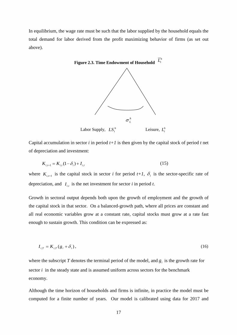
2.4 Labor Supply and Capital Accumulation
The underlying growth rate in the DCGE model is determined by the growth rate of labor and
capital. The labor supply, htLS for each household h is given by the difference between the
household labor endowment, htL , and the demand for leisure, h
tL .
ht
ht
ht LLLS −= . (14)
17
In equilibrium, the wage rate must be such that the labor supplied by the household equals the
total demand for labor derived from the profit maximizing behavior of firms (as set out
above).
Figure 2.3. Time Endowment of Household htL
hLσ
Labor Supply, htLS Leisure, h
tL
Capital accumulation in sector i in period t+1 is then given by the capital stock of period t net
of depreciation and investment:
tiititi IKK ,,1, )1( +−=+ δ (15)
where 1, +tiK is the capital stock in sector i for period t+1, iδ is the sector-specific rate of
depreciation, and tiI , is the net investment for sector i in period t.
Growth in sectoral output depends both upon the growth of employment and the growth of
the capital stock in that sector. On a balanced-growth path, where all prices are constant and
all real economic variables grow at a constant rate, capital stocks must grow at a rate fast
enough to sustain growth. This condition can be expressed as:
)(,, iiTiTi gKI δ+= , (16)
where the subscript T denotes the terminal period of the model, and ig is the growth rate for
sector i in the steady state and is assumed uniform across sectors for the benchmark
economy.
Although the time horizon of households and firms is infinite, in practice the model must be
computed for a finite number of years. Our model is calibrated using data for 2017 and
18
stretches out for 33 years (i.e. through 2050). To ensure that households do not consume the
capital stock prior to the (necessarily arbitrary) end point, a “transversality” condition is
needed, characterizing the “steady state” that is assumed to reign after the end of the time
period under consideration. We assume, following Ramsey (1928) that the economy returns
to the steady state growth rate of 3 percent at the end of the final period T.
The model also requires a number of identities. After-tax income is either consumed or spent
on savings (which equals investment here). Net consumption is defined as gross
consumption spending less any consumption tax. The flow of savings is defined as the
difference between after-tax income and gross spending on consumption, and gross
investment equals national saving plus foreign direct investment.
2.5 Foreign Direct Investment and Capital Inflows
The zero trade balance is a property of a Walrasian general equilibrium model; export or
import prices adjust until the demand equals supply in international markets. However,
foreign direct investment (FDI) plays a crucial role in the U.S. economy as exports and
imports are not automatically balanced by automatic price adjustments. Therefore the
Walrasian model is modified here to incorporate capital inflows so that the FDI can pay for
whenever imports exceed exports.
∑∑ −=i
titii
titit EPEMPMFDI ,,,, (17)
where for period t, tFDI is the amount of net capital inflows into the U.S. economy,
∑i
titi MPM ,, is the volume of imports and ∑i
titi EPE ,, is the volume of exports.
This DCGE model assumes that the FDI is only used to import investment goods. Larger
amounts of FDI increase investment, capital stock, output, utility level and lifetime well-
being of households in the model.

19
2.6 Calibration
The model is truly “dynamic” in that it optimizes the lifetime utility of households and profits
of firms over time, given their constraints, and is calibrated using SAM data for 2017. The
model is programmed in General Algebraic Modeling System (GAMS) along with it
Mathematical Programming for System of General Equilibrium (MPSGE) module, a
specialized program that is widely used for solving DCGE models4.
The dynamics in this model arise from an endogenous process of capital accumulation and
exogenous growth rate of the labor force. We rule out uncertainty and rely on the perfect
foresight of households and firms, which means that actual and expected values of variables
are the same.
There are essentially five steps involved in calibration of this dynamic model. The first step
relates to forming a relation between the price of commodities at period t, tiP , , and the price
of investment good tiPINV , . Then, the composite investment generates capital stock in
period t+1 with price ktiP 1, + . It also needs a link between the prices of the capital stock at
periods t and t+1, ktiP , , tiPINV , and k
tiP 1, + , with due account of the rental on capital and the
depreciation rate. For instance, one unit of investment made using one unit of output in
period t generates one unit of an investment good. This then generates one unit of capital
stock in period t+1. This implies that
ktititi PPINVP 1,,, +⇒⇒ (18)
where tiP , is the price of one output in period t, and tiPINV , and ktiP 1, + are the t period prices
of one unit of investment, and capital goods, in period t+1 in sector i. Capital depreciates at
the rate iδ . One unit of capital at the beginning of period t in sector i earns a rental rate tirk ,
at time t, and ( )iδ−1 units of it remain for the next period (or at the start of the t+1 period),
( ) kti P 11 +−δ . Therefore:
4 MPSGE was written by Thomas Rutherford for further explanation see his paper, “Applied General Equilibrium Modeling with MPSGE as a GAMS Subsystem: An Overview of the Modeling Framework and Syntax”, University of Colorado, 1995; www.gams.com.

20
ktiti
kti PrkP 1,,, )1( +−+= δ (19)
The second step involves setting up a link between the rental rate with the benchmark interest
rate and the depreciation rate; the rental covers depreciation and interest payments for each
unit of investment. If the rental is paid at the end of the period, then:
( ) ktiiti Prrk 1,, ++= δ , (20)
The third step involves forming a relation between the future and the current price of capital,
which is just the benchmark reference price as given by:
rP
Pkti
kti
+=+
11
,
1, . (21)
This means that the ratio of prices of the capital at period t and t+1 equals the market
discount factor, r+1
1 .
The fourth step involves setting up the equilibrium relationship between capital earnings
(value added from capital) and the cost of capital. We compute values for sectoral capital
stocks from sectoral capital earnings in the base year. If capital income in sector i in the base
year is iV , we can write iii KrkV = . Since the return to capital must be sufficient to cover
interest and depreciation, we can also write
iktiii KPrV 1,)( ++= δ or (22)
)( i
ii r
VK
δ+= (23)
with normalization 11 == +k
tt PP .
The fifth step involves setting up the relation between the investment and capital earning on
the balanced growth path. Investment should be enough to provide for growth and
depreciation, iiii KgI )( δ+= , which implies that
ii
iii V
rg
I)()(
δδ
++
= . (24)

21
Thus investment per sector is tied to earnings per sector. In the benchmark equilibrium, all
reference quantities grow at the rate of labor force growth, and reference prices are
discounted on the basis of the benchmark rate of return. The balance between investment and
earnings from capital is restored here by adjustment in the growth rate ig , which responds to
changes in the marginal productivity of capital associated to change in investment.
Readjustment of capital stock and investment continues until this growth rate and the
benchmark interest rates become equal.
If the growth rate in sector i is larger than the benchmark interest rate, then more investment
will be drawn to that sector. The capital stock in that sector rises as more investment takes
place. Eventually, the declining marginal productivity of capital retards growth in that sector.
In addition, the DCGE model builds scenarios for open capital markets and capital inflows to
evaluate the impacts of corporate tax reforms anticipated in 2017.
To solve the model, we allow for a time horizon sufficient enough to approximate the
balanced-growth path for the economy. Currently the model uses a thirty-three year horizon,
which can be increased if the model economy does not converge to the steady state.
3. The Current Tax System and Elasticities
The tax rates currently falling on labor and capital inputs, household income, sales of goods
and services, social security and employment are presented in a set of tables in this section. A
glossary describing the acronyms of the production sectors is available at the end of this
paper.
Table 3.1: Taxes rates on the cost of labor input by sectors
AGRICF 0.0188 MINING 0.0580 CONSTR 0.0106 FOODPR 0.1259
APPARL 0.0584 MFRCON 0.0212 PPAPER 0.0375 CHEMIC 0.0919
ELECTR 0.0288 MVOTRA 0.0637 MFROTH 0.0970 TRANSP 0.0354
INFORM 0.0767 WHOLSA 0.0743 RETAIL 0.0939 BANKNG 0.0646
REALST 0.0052 PROTEC 0.0202 MANGAD 0.0663 HEALTH 0.0071
ENTRHO 0.0160 OTHSVC 0.0116 COMPUT 0.1103 METALS 0.0638
MACHIN 0.1046 UTILIT 0.0192 INSURS 0.0767 Source: Derived from SAM 2017.
22
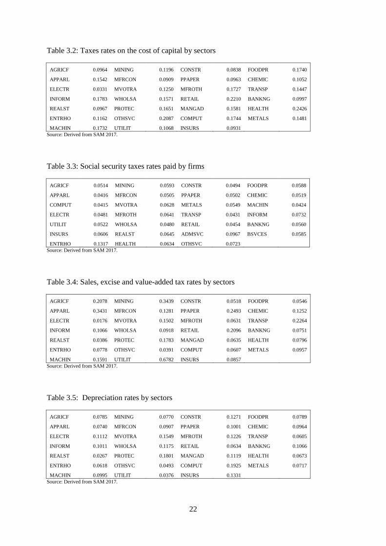
Table 3.2: Taxes rates on the cost of capital by sectors
AGRICF 0.0964 MINING 0.1196 CONSTR 0.0838 FOODPR 0.1740
APPARL 0.1542 MFRCON 0.0909 PPAPER 0.0963 CHEMIC 0.1052
ELECTR 0.0331 MVOTRA 0.1250 MFROTH 0.1727 TRANSP 0.1447
INFORM 0.1783 WHOLSA 0.1571 RETAIL 0.2210 BANKNG 0.0997
REALST 0.0967 PROTEC 0.1651 MANGAD 0.1581 HEALTH 0.2426
ENTRHO 0.1162 OTHSVC 0.2087 COMPUT 0.1744 METALS 0.1481
MACHIN 0.1732 UTILIT 0.1068 INSURS 0.0931 Source: Derived from SAM 2017.
Table 3.3: Social security taxes rates paid by firms
AGRICF 0.0514 MINING 0.0593 CONSTR 0.0494 FOODPR 0.0588
APPARL 0.0416 MFRCON 0.0505 PPAPER 0.0502 CHEMIC 0.0519
COMPUT 0.0415 MVOTRA 0.0628 METALS 0.0549 MACHIN 0.0424
ELECTR 0.0481 MFROTH 0.0641 TRANSP 0.0431 INFORM 0.0732
UTILIT 0.0522 WHOLSA 0.0480 RETAIL 0.0454 BANKNG 0.0560
INSURS 0.0606 REALST 0.0645 ADMSVC 0.0967 BSVCES 0.0585
ENTRHO 0.1317 HEALTH 0.0634 OTHSVC 0.0723 Source: Derived from SAM 2017.
Table 3.4: Sales, excise and value-added tax rates by sectors
AGRICF 0.2078 MINING 0.3439 CONSTR 0.0518 FOODPR 0.0546
APPARL 0.3431 MFRCON 0.1281 PPAPER 0.2493 CHEMIC 0.1252
ELECTR 0.0176 MVOTRA 0.1502 MFROTH 0.0631 TRANSP 0.2264
INFORM 0.1066 WHOLSA 0.0918 RETAIL 0.2096 BANKNG 0.0751
REALST 0.0386 PROTEC 0.1783 MANGAD 0.0635 HEALTH 0.0796
ENTRHO 0.0778 OTHSVC 0.0391 COMPUT 0.0607 METALS 0.0957
MACHIN 0.1591 UTILIT 0.6782 INSURS 0.0857 Source: Derived from SAM 2017.
Table 3.5: Depreciation rates by sectors
AGRICF 0.0785 MINING 0.0770 CONSTR 0.1271 FOODPR 0.0789
APPARL 0.0740 MFRCON 0.0907 PPAPER 0.1001 CHEMIC 0.0964
ELECTR 0.1112 MVOTRA 0.1549 MFROTH 0.1226 TRANSP 0.0605
INFORM 0.1011 WHOLSA 0.1175 RETAIL 0.0634 BANKNG 0.1066
REALST 0.0267 PROTEC 0.1801 MANGAD 0.1119 HEALTH 0.0673
ENTRHO 0.0618 OTHSVC 0.0493 COMPUT 0.1925 METALS 0.0717
MACHIN 0.0995 UTILIT 0.0376 INSURS 0.1331 Source: Derived from SAM 2017.

23
Table 3.6: Social security tax rates by households
DCL1 0.1551 DCL2 0.1551 DCL3 0.1551 DCL4 0.1551 DCL5 0.1551
DCL6 0.1551 DCL7 0.1551 DCL8 0.1551 DCL9 0.1551 DCL10 0.1551 Source: Derived from SAM 2017.
An overview of tax rate figures from Tables 3.1-3.6 above convinces us that that the current
structure of taxes in the US economy is complex. The current system is neither efficient nor
economical, nor good for horizontal or vertical equality among individuals in the US
economy.
3.2 Elasticity parameters
Elasticities of substitution measure the responses of relative changes in quantities to relative
changes prices of goods and services and factors of production in the economy. More flexible
markets have larger values of elasticities. A dynamic CGE model is constructed with sets of
elasticities in consumption, production, trade and inter-temporal choices of households and
firms. Key sets of these elasticities used in the model are provided in the tables in this
section.
Table 3.7: Elasticity of substitution in production
AGRICF 0.9 MINING 0.8 CONSTR 0.9 FOODPR 0.9
APPARL 0.9 MFRCON 0.8 PPAPER 0.8 CHEMIC 0.8
COMPUT 0.9 MVOTRA 0.9 METALS 0.8 MACHIN 0.8
ELECTR 0.9 MFROTH 0.9 TRANSP 0.9 INFORM 0.9
UTILIT 0.8 WHOLSA 0.9 RETAIL 0.9 BANKNG 0.9
INSURS 0.9 REALST 0.9 ADMSVC 0.8 BSVCES 0.8
ENTRHO 0.8 HEALTH 0.8 OTHSVC 0.8 Source: Fair Tax Model, BHT (2015).
Table 3.8: Elasticity of transformation of domestic products in exports
AGRICF 2 MINING 2 CONSTR 2 FOODPR 2
APPARL 2 MFRCON 2 PPAPER 2 CHEMIC 2
COMPUT 2 MVOTRA 2 METALS 2 MACHIN 2
ELECTR 2 MFROTH 2 TRANSP 2 INFORM 2
UTILIT 2 WHOLSA 2 RETAIL 2 BANKNG 2
INSURS 2 REALST 2 ADMSVC 2 BSVCES 2
ENTRHO 2 HEALTH 2 OTHSVC 2 Source: Fair Tax Model, BHT (2015).
24
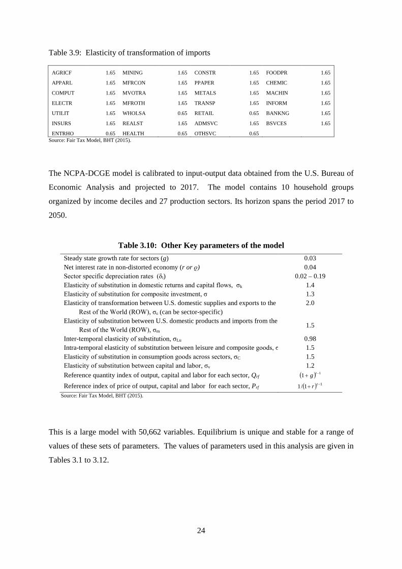
Table 3.9: Elasticity of transformation of imports
AGRICF 1.65 MINING 1.65 CONSTR 1.65 FOODPR 1.65
APPARL 1.65 MFRCON 1.65 PPAPER 1.65 CHEMIC 1.65
COMPUT 1.65 MVOTRA 1.65 METALS 1.65 MACHIN 1.65
ELECTR 1.65 MFROTH 1.65 TRANSP 1.65 INFORM 1.65
UTILIT 1.65 WHOLSA 0.65 RETAIL 0.65 BANKNG 1.65
INSURS 1.65 REALST 1.65 ADMSVC 1.65 BSVCES 1.65
ENTRHO 0.65 HEALTH 0.65 OTHSVC 0.65 Source: Fair Tax Model, BHT (2015).
The NCPA-DCGE model is calibrated to input-output data obtained from the U.S. Bureau of
Economic Analysis and projected to 2017. The model contains 10 household groups
organized by income deciles and 27 production sectors. Its horizon spans the period 2017 to
2050.
Table 3.10: Other Key parameters of the model
Steady state growth rate for sectors (g) 0.03 Net interest rate in non-distorted economy (r or ϱ) 0.04 Sector specific depreciation rates (δi) 0.02 – 0.19 Elasticity of substitution in domestic returns and capital flows, σk 1.4 Elasticity of substitution for composite investment, σ 1.3 Elasticity of transformation between U.S. domestic supplies and exports to the
Rest of the World (ROW), σε (can be sector-specific) 2.0
Elasticity of substitution between U.S. domestic products and imports from the
Rest of the World (ROW), σm 1.5
Inter-temporal elasticity of substitution, σLu 0.98 Intra-temporal elasticity of substitution between leisure and composite goods, σ 1.5 Elasticity of substitution in consumption goods across sectors, σC 1.5 Elasticity of substitution between capital and labor, σv 1.2 Reference quantity index of output, capital and labor for each sector, Qrf ( ) 11 −+ tg
Reference index of price of output, capital and labor for each sector, Prf ( ) 11/1 −+ tr Source: Fair Tax Model, BHT (2015).
This is a large model with 50,662 variables. Equilibrium is unique and stable for a range of
values of these sets of parameters. The values of parameters used in this analysis are given in
Tables 3.1 to 3.12.
25
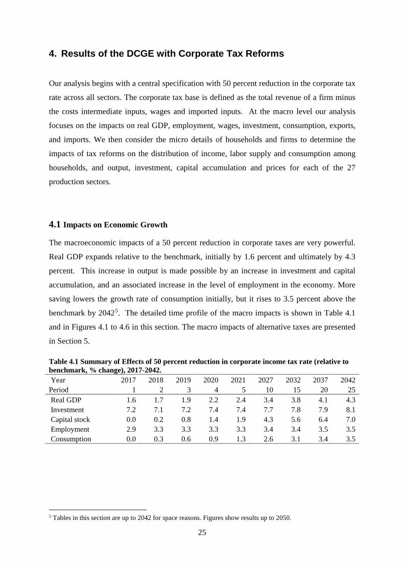
4. Results of the DCGE with Corporate Tax Reforms
Our analysis begins with a central specification with 50 percent reduction in the corporate tax
rate across all sectors. The corporate tax base is defined as the total revenue of a firm minus
the costs intermediate inputs, wages and imported inputs. At the macro level our analysis
focuses on the impacts on real GDP, employment, wages, investment, consumption, exports,
and imports. We then consider the micro details of households and firms to determine the
impacts of tax reforms on the distribution of income, labor supply and consumption among
households, and output, investment, capital accumulation and prices for each of the 27
production sectors.
4.1 Impacts on Economic Growth
The macroeconomic impacts of a 50 percent reduction in corporate taxes are very powerful.
Real GDP expands relative to the benchmark, initially by 1.6 percent and ultimately by 4.3
percent. This increase in output is made possible by an increase in investment and capital
accumulation, and an associated increase in the level of employment in the economy. More
saving lowers the growth rate of consumption initially, but it rises to 3.5 percent above the
benchmark by 20425. The detailed time profile of the macro impacts is shown in Table 4.1
and in Figures 4.1 to 4.6 in this section. The macro impacts of alternative taxes are presented
in Section 5.
Table 4.1 Summary of Effects of 50 percent reduction in corporate income tax rate (relative to benchmark, % change), 2017-2042. Year 2017 2018 2019 2020 2021 2027 2032 2037 2042 Period 1 2 3 4 5 10 15 20 25 Real GDP 1.6 1.7 1.9 2.2 2.4 3.4 3.8 4.1 4.3 Investment 7.2 7.1 7.2 7.4 7.4 7.7 7.8 7.9 8.1 Capital stock 0.0 0.2 0.8 1.4 1.9 4.3 5.6 6.4 7.0 Employment 2.9 3.3 3.3 3.3 3.3 3.4 3.4 3.5 3.5 Consumption 0.0 0.3 0.6 0.9 1.3 2.6 3.1 3.4 3.5
5 Tables in this section are up to 2042 for space reasons. Figures show results up to 2050.

26
Both investment and capital stock keep rising under the tax-change scenario relative to
benchmark as shown on Figures 4.3 and 4.4. GDP is above the benchmark economy for most
of the years. This is possible because of the increase in capital accumulation that raises the
productivity of workers. Similarly, total employment also rises in the beginning relative to
the benchmark because the abundantly available capital results in more demand for labor.
Total investment also follows the pattern of total output.
0
15
30
45
60
75
90
105
120
135
150
2017
2022
2027
2032
2037
2042
2047
Trill
ion
USD
Figure 4.1: Level of real GDP
without reforms
With tax reforms
97
98
99
100
101
102
103
104
105
106
2017
2022
2027
2032
2037
2042
2047
Inde
x
Figure 4.2: Real output under the tax reforms relative to the benchmark
without reforms
With tax reforms

27
94
96
98
100
102
104
106
108
110
2017
2022
2027
2032
2037
2042
2047
Inde
x
Figure 4.3: Investment under the tax reforms relative to the benchmark
without reforms
With tax reforms
94
96
98
100
102
104
106
108
110
2017
2022
2027
2032
2037
2042
2047
Inde
x
Figure 4.4: Capital stock under the tax reforms relative to the benchmark
without reforms
With tax reforms

28
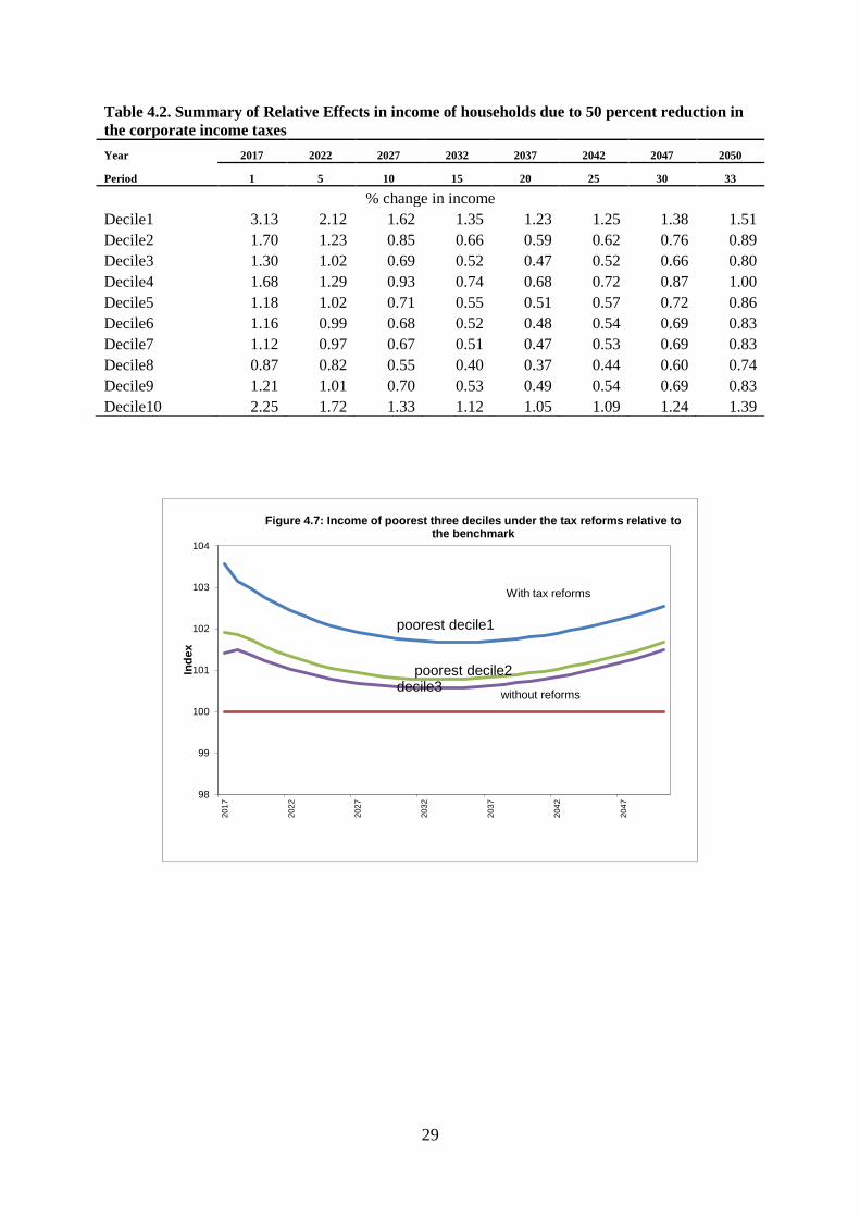
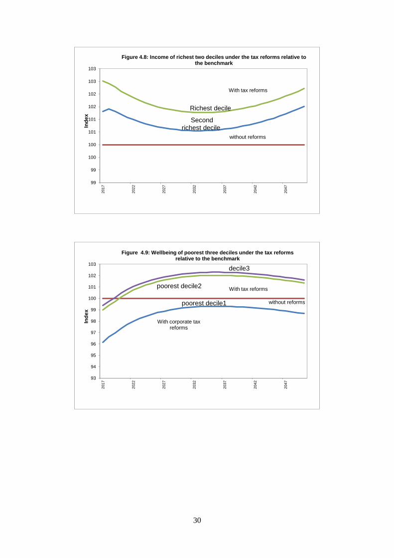
4.2 Impacts on the distribution of income
The income of households rises under the rate reduction as shown in table 4.2. Thus the
redistributive impacts of reforms are very encouraging (See Figures 4.7-4.8.).
97
98
99
100
101
102
103
104
105
2017
2022
2027
2032
2037
2042
2047
Inde
x
Figure 4.5: Employment under the tax reforms relative to the benchmark
without reforms
With tax reforms
98
99
100
101
102
103
104
2017
2022
2027
2032
2037
2042
2047
Inde
x
Figure 4.6: Consumption under the tax reforms relative to the benchmark
without reforms
With tax reforms
29
Table 4.2. Summary of Relative Effects in income of households due to 50 percent reduction in the corporate income taxes Year 2017 2022 2027 2032 2037 2042 2047 2050
Period 1 5 10 15 20 25 30 33
% change in income Decile1 3.13 2.12 1.62 1.35 1.23 1.25 1.38 1.51 Decile2 1.70 1.23 0.85 0.66 0.59 0.62 0.76 0.89 Decile3 1.30 1.02 0.69 0.52 0.47 0.52 0.66 0.80 Decile4 1.68 1.29 0.93 0.74 0.68 0.72 0.87 1.00 Decile5 1.18 1.02 0.71 0.55 0.51 0.57 0.72 0.86 Decile6 1.16 0.99 0.68 0.52 0.48 0.54 0.69 0.83 Decile7 1.12 0.97 0.67 0.51 0.47 0.53 0.69 0.83 Decile8 0.87 0.82 0.55 0.40 0.37 0.44 0.60 0.74 Decile9 1.21 1.01 0.70 0.53 0.49 0.54 0.69 0.83 Decile10 2.25 1.72 1.33 1.12 1.05 1.09 1.24 1.39
poorest decile1
poorest decile2decile3
98
99
100
101
102
103
104
2017
2022
2027
2032
2037
2042
2047
Inde
x
Figure 4.7: Income of poorest three deciles under the tax reforms relative to the benchmark
without reforms
With tax reforms
30
Second richest decile
Richest decile
99
99
100
100
101
101
102
102
103
103
2017
2022
2027
2032
2037
2042
2047
Inde
x
Figure 4.8: Income of richest two deciles under the tax reforms relative to the benchmark
without reforms
With tax reforms
poorest decile1
poorest decile2
decile3
93
94
95
96
97
98
99
100
101
102
103
2017
2022
2027
2032
2037
2042
2047
Inde
x
Figure 4.9: Wellbeing of poorest three deciles under the tax reforms relative to the benchmark
without reforms
With tax reforms
With corporate tax reforms
31
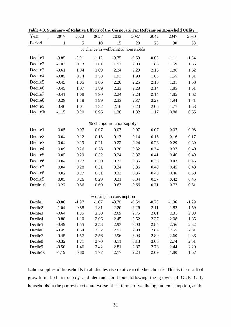
Table 4.3. Summary of Relative Effects of the Corporate Tax Reforms on Household Utility Year 2017 2022 2027 2032 2037 2042 2047 2050 Period 1 5 10 15 20 25 30 33
% change in wellbeing of households
Decile1 -3.85 -2.01 -1.12 -0.75 -0.69 -0.83 -1.11 -1.34 Decile2 -1.03 0.73 1.61 1.97 2.03 1.88 1.59 1.36 Decile3 -0.61 1.04 1.89 2.24 2.29 2.15 1.86 1.62 Decile4 -0.85 0.74 1.58 1.93 1.98 1.83 1.55 1.31 Decile5 -0.45 1.05 1.86 2.20 2.25 2.10 1.81 1.58 Decile6 -0.45 1.07 1.89 2.23 2.28 2.14 1.85 1.61 Decile7 -0.41 1.08 1.90 2.24 2.28 2.14 1.85 1.62 Decile8 -0.28 1.18 1.99 2.33 2.37 2.23 1.94 1.71 Decile9 -0.46 1.01 1.82 2.16 2.20 2.06 1.77 1.53 Decile10 -1.15 0.20 0.96 1.28 1.32 1.17 0.88 0.65
% change in labor supply Decile1 0.05 0.07 0.07 0.07 0.07 0.07 0.07 0.08 Decile2 0.04 0.12 0.13 0.13 0.14 0.15 0.16 0.17 Decile3 0.04 0.19 0.21 0.22 0.24 0.26 0.29 0.30 Decile4 0.09 0.26 0.28 0.30 0.32 0.34 0.37 0.40 Decile5 0.05 0.29 0.32 0.34 0.37 0.41 0.46 0.49 Decile6 0.04 0.27 0.30 0.32 0.35 0.38 0.43 0.46 Decile7 0.04 0.28 0.31 0.34 0.36 0.40 0.45 0.48 Decile8 0.02 0.27 0.31 0.33 0.36 0.40 0.46 0.50 Decile9 0.05 0.26 0.29 0.31 0.34 0.37 0.42 0.45 Decile10 0.27 0.56 0.60 0.63 0.66 0.71 0.77 0.81
% change in consumption Decile1 -3.86 -1.97 -1.07 -0.70 -0.64 -0.78 -1.06 -1.29 Decile2 -1.04 0.88 1.81 2.20 2.26 2.11 1.82 1.59 Decile3 -0.64 1.35 2.30 2.69 2.75 2.61 2.31 2.08 Decile4 -0.88 1.10 2.06 2.45 2.52 2.37 2.08 1.85 Decile5 -0.49 1.55 2.53 2.93 3.00 2.85 2.56 2.32 Decile6 -0.49 1.54 2.52 2.92 2.98 2.84 2.55 2.31 Decile7 -0.45 1.57 2.56 2.96 3.03 2.89 2.60 2.36 Decile8 -0.32 1.71 2.70 3.11 3.18 3.03 2.74 2.51 Decile9 -0.50 1.46 2.42 2.81 2.87 2.73 2.44 2.20 Decile10 -1.19 0.80 1.77 2.17 2.24 2.09 1.80 1.57
Labor supplies of households in all deciles rise relative to the benchmark. This is the result of
growth in both in supply and demand for labor following the growth of GDP. Only
households in the poorest decile are worse off in terms of wellbeing and consumption, as the
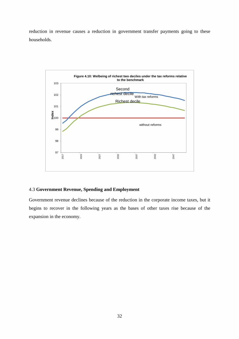
32
reduction in revenue causes a reduction in government transfer payments going to these
households.
4.3 Government Revenue, Spending and Employment
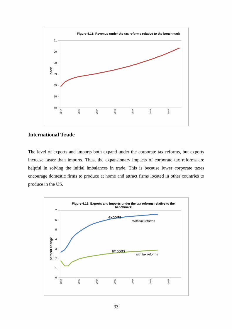
Government revenue declines because of the reduction in the corporate income taxes, but it
begins to recover in the following years as the bases of other taxes rise because of the
expansion in the economy.
Second richest decile
Richest decile
97
98
99
100
101
102
103
2017
2022
2027
2032
2037
2042
2047
Inde
x
Figure 4.10: Welbeing of richest two deciles under the tax reforms relative to the benchmark
without reforms
With tax reforms
33
International Trade
The level of exports and imports both expand under the corporate tax reforms, but exports
increase faster than imports. Thus, the expansionary impacts of corporate tax reforms are
helpful in solving the initial imbalances in trade. This is because lower corporate taxes
encourage domestic firms to produce at home and attract firms located in other countries to
produce in the US.
88
88
89
89
90
90
91
2017
2022
2027
2032
2037
2042
2047
Inde
x
Figure 4.11: Revenue under the tax reforms relative to the benchmark
exports
Imports
0
1
2
3
4
5
6
7
2017
2022
2027
2032
2037
2042
2047
perc
ent c
hang
e
Figure 4.12: Exports and imports under the tax reforms relative to the benchmark
with tax reforms
With tax reforms
34
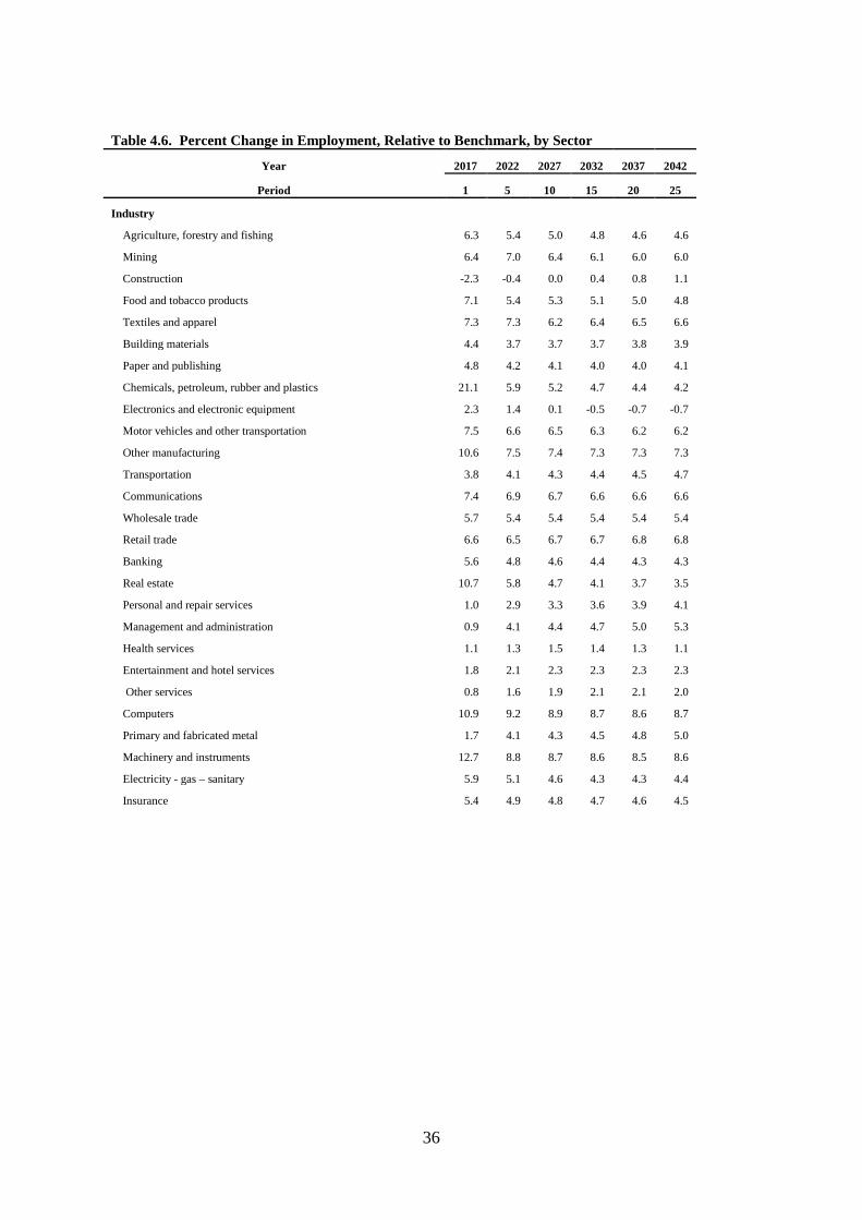
4.5 Sectoral analysis Every sector is growing faster with the reforms in the corporate income taxes than without
reforms. The machinery and instrument, real estate, and computer sectors grow faster than
any other sectors. These sectoral growth rates come mainly from the increased stock of
capital across sectors and the creation of more jobs across sectors. Under this reform
experiment, the construction sector grows the least among all sectors, this is a puzzle that will
be investigated further.
Table 4.4. Percent Change in Real Output, Relative to Benchmark, by Sector
Year 2017 2022 2027 2032 2037 2042
Period 1 5 10 15 20 25 Industry
Agriculture, forestry and fishing 2.9 4.4 5.1 5.4 5.6 5.7 Mining 3.5 5.5 6.4 6.8 7.1 7.4 Construction -2.5 -1.0 -0.2 0.3 0.8 1.2 Food and tobacco products 0.8 2.7 3.6 4.0 4.1 4.1 Textiles and apparel 2.3 3.4 4.7 5.0 5.1 5.1 Building materials 1.8 2.7 3.4 3.7 3.9 4.1 Paper and publishing 2.2 2.9 3.5 3.8 4.0 4.2 Chemicals, petroleum, rubber and plastics 1.6 3.9 5.0 5.6 6.0 6.2 Electronics and electronic equipment 0.4 0.7 1.3 1.8 2.2 2.6 Motor vehicles and other transportation 3.4 3.9 4.5 4.8 4.9 5.0 Other manufacturing 1.7 4.1 4.6 4.8 4.8 4.8 Transportation 2.8 3.4 3.9 4.1 4.2 4.3 Communications 3.7 4.0 4.5 4.7 4.8 4.9 Wholesale trade 2.3 3.0 3.6 3.9 4.0 4.0 Retail trade 2.5 4.4 4.7 4.6 4.5 4.4 Banking 2.5 3.3 4.0 4.4 4.6 4.7 Real estate 1.4 4.8 5.9 6.4 6.8 7.1 Personal and repair services 0.8 1.2 1.8 2.1 2.3 2.5 Management and administration 1.5 2.3 3.0 3.4 3.7 3.9 Health services 0.8 1.1 1.2 1.1 0.9 0.7 Entertainment and hotel services 1.1 1.7 2.2 2.4 2.4 2.4
Other services 0.7 1.5 1.8 1.9 1.9 1.8 Computers 2.7 5.0 5.4 5.6 5.7 5.8 Primary and fabricated metal 1.8 2.8 3.6 4.1 4.4 4.7 Machinery and instruments 5.4 7.2 7.4 7.4 7.4 7.4 Electricity - gas – sanitary 3.5 4.6 5.3 5.7 6.1 6.4 Insurance 1.2 2.9 4.3 5.0 5.4 5.5
The demand and supply for products in the markets increase because of the rise in the income
of households and more investment by firms, leading to expansion across all sectors. The
sectors that are more efficient attract more capital and create more jobs and grow faster. The
underlying elasticities of substitution in consumption, production and trade also matter for the
flexibility of markets and growth rates across these sectors.
35
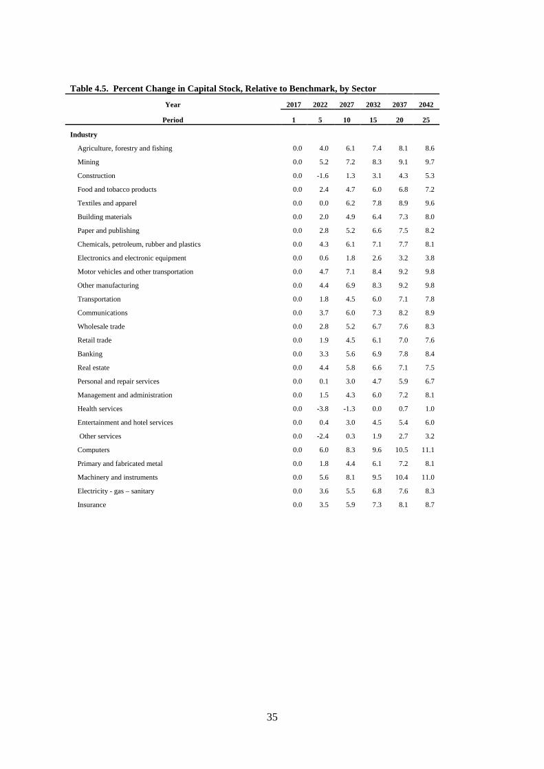
Table 4.5. Percent Change in Capital Stock, Relative to Benchmark, by Sector
Year 2017 2022 2027 2032 2037 2042
Period 1 5 10 15 20 25
Industry
Agriculture, forestry and fishing 0.0 4.0 6.1 7.4 8.1 8.6
Mining 0.0 5.2 7.2 8.3 9.1 9.7
Construction 0.0 -1.6 1.3 3.1 4.3 5.3
Food and tobacco products 0.0 2.4 4.7 6.0 6.8 7.2
Textiles and apparel 0.0 0.0 6.2 7.8 8.9 9.6
Building materials 0.0 2.0 4.9 6.4 7.3 8.0
Paper and publishing 0.0 2.8 5.2 6.6 7.5 8.2
Chemicals, petroleum, rubber and plastics 0.0 4.3 6.1 7.1 7.7 8.1
Electronics and electronic equipment 0.0 0.6 1.8 2.6 3.2 3.8
Motor vehicles and other transportation 0.0 4.7 7.1 8.4 9.2 9.8
Other manufacturing 0.0 4.4 6.9 8.3 9.2 9.8
Transportation 0.0 1.8 4.5 6.0 7.1 7.8
Communications 0.0 3.7 6.0 7.3 8.2 8.9
Wholesale trade 0.0 2.8 5.2 6.7 7.6 8.3
Retail trade 0.0 1.9 4.5 6.1 7.0 7.6
Banking 0.0 3.3 5.6 6.9 7.8 8.4
Real estate 0.0 4.4 5.8 6.6 7.1 7.5
Personal and repair services 0.0 0.1 3.0 4.7 5.9 6.7
Management and administration 0.0 1.5 4.3 6.0 7.2 8.1
Health services 0.0 -3.8 -1.3 0.0 0.7 1.0
Entertainment and hotel services 0.0 0.4 3.0 4.5 5.4 6.0
Other services 0.0 -2.4 0.3 1.9 2.7 3.2
Computers 0.0 6.0 8.3 9.6 10.5 11.1
Primary and fabricated metal 0.0 1.8 4.4 6.1 7.2 8.1
Machinery and instruments 0.0 5.6 8.1 9.5 10.4 11.0
Electricity - gas – sanitary 0.0 3.6 5.5 6.8 7.6 8.3
Insurance 0.0 3.5 5.9 7.3 8.1 8.7
36
Table 4.6. Percent Change in Employment, Relative to Benchmark, by Sector
Year 2017 2022 2027 2032 2037 2042
Period 1 5 10 15 20 25
Industry
Agriculture, forestry and fishing 6.3 5.4 5.0 4.8 4.6 4.6
Mining 6.4 7.0 6.4 6.1 6.0 6.0
Construction -2.3 -0.4 0.0 0.4 0.8 1.1
Food and tobacco products 7.1 5.4 5.3 5.1 5.0 4.8
Textiles and apparel 7.3 7.3 6.2 6.4 6.5 6.6
Building materials 4.4 3.7 3.7 3.7 3.8 3.9
Paper and publishing 4.8 4.2 4.1 4.0 4.0 4.1
Chemicals, petroleum, rubber and plastics 21.1 5.9 5.2 4.7 4.4 4.2
Electronics and electronic equipment 2.3 1.4 0.1 -0.5 -0.7 -0.7
Motor vehicles and other transportation 7.5 6.6 6.5 6.3 6.2 6.2
Other manufacturing 10.6 7.5 7.4 7.3 7.3 7.3
Transportation 3.8 4.1 4.3 4.4 4.5 4.7
Communications 7.4 6.9 6.7 6.6 6.6 6.6
Wholesale trade 5.7 5.4 5.4 5.4 5.4 5.4
Retail trade 6.6 6.5 6.7 6.7 6.8 6.8
Banking 5.6 4.8 4.6 4.4 4.3 4.3
Real estate 10.7 5.8 4.7 4.1 3.7 3.5
Personal and repair services 1.0 2.9 3.3 3.6 3.9 4.1
Management and administration 0.9 4.1 4.4 4.7 5.0 5.3
Health services 1.1 1.3 1.5 1.4 1.3 1.1
Entertainment and hotel services 1.8 2.1 2.3 2.3 2.3 2.3
Other services 0.8 1.6 1.9 2.1 2.1 2.0
Computers 10.9 9.2 8.9 8.7 8.6 8.7
Primary and fabricated metal 1.7 4.1 4.3 4.5 4.8 5.0
Machinery and instruments 12.7 8.8 8.7 8.6 8.5 8.6
Electricity - gas – sanitary 5.9 5.1 4.6 4.3 4.3 4.4
Insurance 5.4 4.9 4.8 4.7 4.6 4.5
37
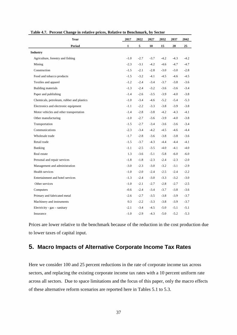
Table 4.7. Percent Change in relative prices, Relative to Benchmark, by Sector
Year 2017 2022 2027 2032 2037 2042
Period 1 5 10 15 20 25
Industry
Agriculture, forestry and fishing -1.0 -2.7 -3.7 -4.2 -4.3 -4.2
Mining -2.3 -3.1 -4.2 -4.6 -4.7 -4.7
Construction -1.5 -2.1 -2.8 -3.0 -3.0 -2.8
Food and tobacco products -1.5 -3.2 -4.1 -4.5 -4.6 -4.5
Textiles and apparel -1.2 -2.4 -3.4 -3.7 -3.8 -3.6
Building materials -1.3 -2.4 -3.2 -3.6 -3.6 -3.4
Paper and publishing -1.4 -2.6 -3.5 -3.9 -4.0 -3.8
Chemicals, petroleum, rubber and plastics -1.0 -3.4 -4.6 -5.2 -5.4 -5.3
Electronics and electronic equipment -1.1 -2.2 -3.3 -3.8 -3.9 -3.8
Motor vehicles and other transportation -1.4 -2.8 -3.8 -4.2 -4.3 -4.1
Other manufacturing -1.0 -2.7 -3.6 -3.9 -4.0 -3.8
Transportation -1.5 -2.7 -3.4 -3.6 -3.6 -3.4
Communications -2.3 -3.4 -4.2 -4.5 -4.6 -4.4
Wholesale trade -1.7 -2.8 -3.6 -3.8 -3.8 -3.6
Retail trade -1.5 -3.7 -4.3 -4.4 -4.4 -4.1
Banking -1.1 -2.5 -3.5 -4.0 -4.1 -4.0
Real estate 1.3 -3.6 -5.1 -5.8 -6.0 -6.0
Personal and repair services -1.8 -1.8 -2.3 -2.4 -2.3 -2.0
Management and administration -3.0 -2.3 -3.0 -3.2 -3.1 -2.9
Health services -1.0 -2.0 -2.4 -2.5 -2.4 -2.2
Entertainment and hotel services -1.3 -2.4 -3.0 -3.3 -3.2 -3.0
Other services -1.0 -2.1 -2.7 -2.8 -2.7 -2.5
Computers -0.6 -2.4 -3.4 -3.7 -3.8 -3.6
Primary and fabricated metal -2.6 -2.7 -3.5 -3.8 -3.9 -3.7
Machinery and instruments 0.3 -2.2 -3.3 -3.8 -3.9 -3.7
Electricity - gas – sanitary -2.1 -3.4 -4.5 -5.0 -5.1 -5.1
Insurance -1.0 -2.9 -4.3 -5.0 -5.2 -5.3 Prices are lower relative to the benchmark because of the reduction in the cost production due
to lower taxes of capital input.
5. Macro Impacts of Alternative Corporate Income Tax Rates
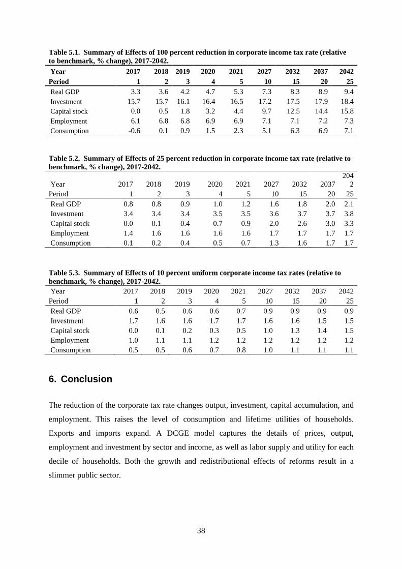
Here we consider 100 and 25 percent reductions in the rate of corporate income tax across
sectors, and replacing the existing corporate income tax rates with a 10 percent uniform rate
across all sectors. Due to space limitations and the focus of this paper, only the macro effects
of these alternative reform scenarios are reported here in Tables 5.1 to 5.3.
38
Table 5.1. Summary of Effects of 100 percent reduction in corporate income tax rate (relative to benchmark, % change), 2017-2042. Year 2017 2018 2019 2020 2021 2027 2032 2037 2042 Period 1 2 3 4 5 10 15 20 25 Real GDP 3.3 3.6 4.2 4.7 5.3 7.3 8.3 8.9 9.4 Investment 15.7 15.7 16.1 16.4 16.5 17.2 17.5 17.9 18.4 Capital stock 0.0 0.5 1.8 3.2 4.4 9.7 12.5 14.4 15.8 Employment 6.1 6.8 6.8 6.9 6.9 7.1 7.1 7.2 7.3 Consumption -0.6 0.1 0.9 1.5 2.3 5.1 6.3 6.9 7.1 Table 5.2. Summary of Effects of 25 percent reduction in corporate income tax rate (relative to benchmark, % change), 2017-2042.
Year 2017 2018 2019 2020 2021 2027 2032 2037 204
2 Period 1 2 3 4 5 10 15 20 25 Real GDP 0.8 0.8 0.9 1.0 1.2 1.6 1.8 2.0 2.1 Investment 3.4 3.4 3.4 3.5 3.5 3.6 3.7 3.7 3.8 Capital stock 0.0 0.1 0.4 0.7 0.9 2.0 2.6 3.0 3.3 Employment 1.4 1.6 1.6 1.6 1.6 1.7 1.7 1.7 1.7 Consumption 0.1 0.2 0.4 0.5 0.7 1.3 1.6 1.7 1.7
Table 5.3. Summary of Effects of 10 percent uniform corporate income tax rates (relative to benchmark, % change), 2017-2042. Year 2017 2018 2019 2020 2021 2027 2032 2037 2042 Period 1 2 3 4 5 10 15 20 25 Real GDP 0.6 0.5 0.6 0.6 0.7 0.9 0.9 0.9 0.9 Investment 1.7 1.6 1.6 1.7 1.7 1.6 1.6 1.5 1.5 Capital stock 0.0 0.1 0.2 0.3 0.5 1.0 1.3 1.4 1.5 Employment 1.0 1.1 1.1 1.2 1.2 1.2 1.2 1.2 1.2 Consumption 0.5 0.5 0.6 0.7 0.8 1.0 1.1 1.1 1.1
6. Conclusion
The reduction of the corporate tax rate changes output, investment, capital accumulation, and
employment. This raises the level of consumption and lifetime utilities of households.
Exports and imports expand. A DCGE model captures the details of prices, output,
employment and investment by sector and income, as well as labor supply and utility for each
decile of households. Both the growth and redistributional effects of reforms result in a
slimmer public sector.
39
The model is also able to identify the complexity of the current tax system with detailed
information on labor, and capital input taxes across sector, and sales, household income and
social security taxes.
7. References
Angelini J. P. and D.G. Tuerck. 2015. The U.S. Corporate Income Tax: A Primer for U.S. Policymakers. The Beacon Hill Institute at Suffolk University. http://www.ncpa.org/pdfs/sp_The%20U.S.%20Corporate%20Income%20Tax.pdf.
Arulampalam, W., M. P. Devereux, and G. Maffini. 2012. The Direct Incidence of Corporate Income Tax on Wages. European Economic Review, 56(6), 1038-1054.
Bhattarai K., J. Haughton and D.G. Tuerck. 2015. Fiscal Policy, Growth and Income
Distribution in the UK, Applied Economics and Finance (2:3):20-36.
Bhattarai K., J. Haughton and D.G. Tuerck (2015) The Economic Effects of the Fair Tax: Analysis of Results of a Dynamic CGE Model of the US Economy, International Economics and Economic Policy, forthcoming.
Hall, R.E. and A, Rabushka. 1985. The Flat Tax, Hoover Press.
Leibrecht, M. and C. Hochgatterer. 2012. Tax Competition as a Cause of Falling Corporate Income Tax Rates: A Survey of Empirical Literature. Journal of Economic Surveys, (26)4: 616-48.
Mirrlees J., S., Adam, T., Besley, R., Blundell, S., Bond, R., Chote, M., Gammie, P. J., Myles, G., & Poterba, J. 2010, Dimensions of Tax Design: The Mirrlees Review, Oxford: Oxford University Press.
Overesch, M. and J. Rincke, 2011. What Drives Corporate Tax Rates Down? A Reassessment of Globalization, Tax Competition, and Dynamic Adjustment to Shocks. The Scandinavian Journal of Economics, 113: 579–602. doi: 10.1111/j.1467-9442.2011.01650.x.
U.S. Council of Economic Advisers. 2015. Economic Report of the President, U.S. Government Printing Office, Washington DC.
Zellner, A., and J.K. Ngoie. 2015. Evaluation of the Effects of Reduced Personal and Corporate Tax Rates on the Growth Rates of the U.S. Economy Econometric Reviews 34, (1-5):56-81.
40
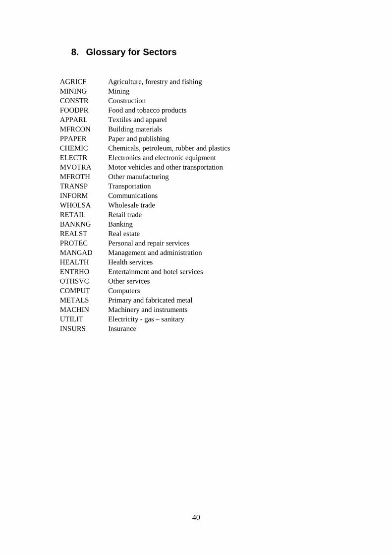
8. Glossary for Sectors
AGRICF Agriculture, forestry and fishing MINING Mining
CONSTR Construction FOODPR Food and tobacco products APPARL Textiles and apparel MFRCON Building materials PPAPER Paper and publishing CHEMIC Chemicals, petroleum, rubber and plastics ELECTR Electronics and electronic equipment MVOTRA Motor vehicles and other transportation MFROTH Other manufacturing TRANSP Transportation INFORM Communications WHOLSA Wholesale trade RETAIL Retail trade BANKNG Banking
REALST Real estate PROTEC Personal and repair services MANGAD Management and administration HEALTH Health services ENTRHO Entertainment and hotel services OTHSVC Other services COMPUT Computers
METALS Primary and fabricated metal MACHIN Machinery and instruments UTILIT Electricity - gas – sanitary INSURS Insurance