simulating and estimating dsge model with dynare›¾涛-dyanre-slides.pdf · simulating and...

Simulating and Estimating DSGE Model with Dynare

Tao Zeng

Wuhan University

April 2016

SEM (Institute) Short Couse 04/28 1 / 68

What is Dynare?

Dynare is a Matlab frontend to solve and simulate dynamic models

Either deterministic or stochastic

Developed by Michel Juillard at CEPREMAP

website: http://www.cepremap.cnrs.fr/dynare/


How does it work?

Write the code of the model

Takes care of parsing the model to Dynare

Rearrange the model

Solves the model

Use the solution to generate some output

Can estimate the model


Structure of the mod file: Simulation

Preamble: Define variables and parameters

Model: Equations of the model

Steady State: Compute the steady state

Shocks: Define the properties of Shocks

Solution: Compute the Solution and Product Output


Structure of the mod file: Preamble

In this part, we need to define endogenous variables, shocks andparameters by three commands var, varexo and parameters.

VAR: define the endogenous variables of your modelVAREXO: define the list of shocks in your modelPARAMETERS: define the list of parameters and then assign theparameters values.

Assume the model takes the form

xt = ρxt−1 + et

with et ∼ N(0, σ2

).

Variable is xt , exogenous variables is et and parameters are ρ and σ.


Structure of the mod file: PreambleMotivated Example: Match

In practice, we always want to know wether our model match data

The model takes the form

xt = ρxt−1 + et

with et ∼ N(0, σ2

).

We compute the sample moments such as mean, variance andcovariance of the data.

Then we compute the theoretical moments of the model.

Compare the sample moments with the theoretical moments.

Here we simulate data from the model, treat the simulated data asreal data and compute the moments such as mean, variance andcovariance.


Structure of the mod file: PreambleAn example

The dynare code for the Preamble part

var x;varexo e;

parameters rho,se;rho = 0.90;se = 0.01;


Structure of the mod file: ModelAn example

In the model block, we need to define model equations using"model;" and "end;"

Model the AR(1) processes asmodel;x=rho*x(-1)+e;end;

Between the command model and end, there need to be as manyequations as you declared endogenous variables in the var part.Each line of instruction ends with a semicolon.

Variable with a time t subscript, such as xt ,is written as x .

Variable with a time t-n subscript, such as xt−n, is written as x (−n).Variable with a time t+n subscript, such as xt+n, is written as x (+n).


Structure of the mod file: Steady State

Compute the long—run of the model which is the deterministic valuethat the dynamic system will converge to.

We will take appximation around this long run.

The structure is as follows

inival;· · ·end;steady;check;

Steady computes the long run of the model using a non—linearNew-type solver.

It therefore needs initial conditions. That is the role of theinival ;· · · end ; statement. Note that if the inival block is not followedby steady, the steady state computation will still be triggered bysubsequent commands (stoch_simul, estimation,...).



You would better give a initial value close to the exact steady state.

histval;...end; block allows setting the starting point of thosesimulations in the state space (it does not affect the starting point forimpulse response functions).histval;x(0)=0;end;

check is optional. It checks the dynamic stability of the system by BKcondition. It computes and displays the eigenvalues of the system. Anecessary conditions for the uniqueness of a stable equilibrium in theneighborhood of the steady state is that there are as manyeigenvalues larger than 1 in modulus as there are forward lookingvariables in the system.



Again take the AR(1) example:

xt = ρxt−1 + et

In deterministic steady state: et = e = 0, therefore

x = ρx =⇒ x = 0

Henceinitivale = 0x = 0end;steady;check;


Structure of the mod file: Shocks

Exogenous shocks are gaussian innovations with 0 mean.

Structure:shocks;var ...;stderr ...;

Therefore, for the AR(1) exampleshocks;var e;stderr se;end;


Structure of the mod file: Solution

Final step: Compute the solution and produce some output

Solution method: First or Second order perturbation method

Then compute some moments and impulse responses.

Getting solution: stoch_simul(...)...;

Again take the AR(1) example: xt = ρxt−1 + etTherefore (because the model is linear): stoch_simul(linear);


Structure of the mod file: SolutionOptions of the stoch_simul

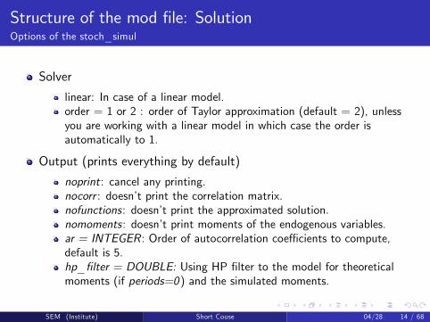
Solver

linear: In case of a linear model.order = 1 or 2 : order of Taylor approximation (default = 2), unlessyou are working with a linear model in which case the order isautomatically to 1.

Output (prints everything by default)

noprint: cancel any printing.nocorr : doesn’t print the correlation matrix.nofunctions: doesn’t print the approximated solution.nomoments: doesn’t print moments of the endogenous variables.ar = INTEGER: Order of autocorrelation coeffi cients to compute,default is 5.hp_filter = DOUBLE: Using HP filter to the model for theoreticalmoments (if periods=0) and the simulated moments.



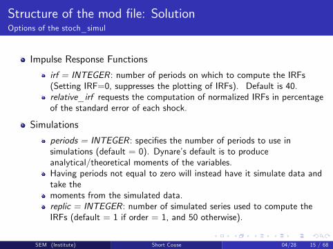
Impulse Response Functions

irf = INTEGER : number of periods on which to compute the IRFs(Setting IRF=0, suppresses the plotting of IRFs). Default is 40.relative_irf requests the computation of normalized IRFs in percentageof the standard error of each shock.

Simulations

periods = INTEGER: specifies the number of periods to use insimulations (default = 0). Dynare’s default is to produceanalytical/theoretical moments of the variables.Having periods not equal to zero will instead have it simulate data andtake themoments from the simulated data.replic = INTEGER: number of simulated series used to compute theIRFs (default = 1 if order = 1, and 50 otherwise).



Simulations

drop = INTEGER : number of points dropped in simulations (default =100). By default, Dynare drops the first 100 values from a simulation,so you need to give it a number of periods greater than 100 for this towork. Hence, typing “stoch simul(periods=300);”will producemoments based on a simulation with 200 periods.set_dynare_seed (INTEGER): set the random seeds

To run a Dynare file, simply type "dynare filename" into thecommand window while in Matlab. For e.g.: "dynare *.mod"


Structure of the mod file: Some tipsLog-linearized: Neoclassical example

Dynare obtains linear approximations to the policy functions thatsatisfy the first-order conditions.

State variables: xt = [x1t , x2t , · · · , xnt ]′

The endogenous variable can be expressed as

yt = y + a (xt − x)

where a bar above a variable indicates steady state value.


Structure of the mod file: Some tipsNeoclassical example

Specification of the model in level

max{ct ,kt}∞

t=1

E∞

∑t=1

βt−1c1−vt − 11− v

ct + kt+1 = ztkαt−1 + (1− δ) kt−1

zt = (1− ρ) + ρzt−1 + εt

k0 given, Et (εt+1) = 0 and Et(ε2t+1

)= σ2

Model equations

c−vt = Et[βc−vt+1

(αzt+1kα−1

t + 1− δ)]

ct + kt = ztkαt−1 + (1− δ) kt−1

zt = (1− ρ) + ρzt−1 + εt



xt = [kt−1, zt ], yt = [ct , kt , zt ]

Linearized solution

ct = c + ack (kt−1 − k) + acz (zt − z) (1)

kt = k + akk (kt−1 − k) + akz (zt − z) (2)

zt = ρzt−1 + εt (3)

Dynare does not understand what ct is, it only generates a linearsolution in what you specify as the variables.



The equation (2) and (3) can of course be written (less conveniently)as

kt = k + akk (kt−1 − k) + akz−1 (zt−1 − z) + akz εt

zt = ρzt−1 + εt

by substituting (3) into (2) with akz−1 = ρakz .

Dynare gives the solution in the less convenient form

ct = c + ack (kt−1 − k) + acz−1 (zt−1 − z) + acz εt

kt = k + akk (kt−1 − k) + akz−1 (zt−1 − z) + akz εt

zt = ρzt−1 + εt



Dynare equations

c^(-nu)=beta*c(+1)^(-nu)*(alpha*z(+1)*k^(alpha-1)+1-delta);c+k=z*k(-1)^alpha+(1-delta)k(-1);

z=(1-rho)+rho*z(-1)+e;

δ = 0.025, v = 2, α = 0.36, β = 0.99, and ρ = 0.95 and the resultsfrom the dynare

POLICY AND TRANSITION FUNCTIONSk z c

constant 37.989254 1.000000 2.754327k(-1) 0.976540 -0.000000 0.033561z(-1) 2.597386 0.950000 0.921470e 2.734091 1.000000 0.969968



The table must be interpreted as follows

k z cconstant 37.989254 1.000000 2.754327k(-1)-kss 0.976540 -0.000000 0.033561z(-1)-zss 2.597386 0.950000 0.921470e 2.734091 1.000000 0.969968

That is, explanatory variables are relative to steady state. (Note thatsteady state of e is zero by definition)

If explanatory variables take on steady state values, then choices areequal to the constant term, which of course is simply equal to thecorresponding steady state value



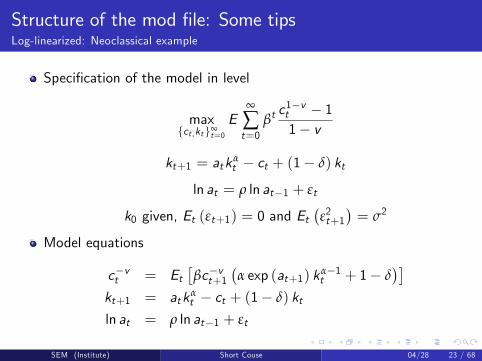
Specification of the model in level

max{ct ,kt}∞

t=0

E∞

∑t=0

βtc1−vt − 11− v

kt+1 = atkαt − ct + (1− δ) kt

ln at = ρ ln at−1 + εt

k0 given, Et (εt+1) = 0 and Et(ε2t+1

)= σ2

Model equations


(α exp (at+1) kα−1

t + 1− δ)]

kt+1 = atkαt − ct + (1− δ) kt




In particular, Dynare requires that predetermined variables (like thecaptical stock) show up as dated t − 1 in the time t equatiion and tin the tiime t + 1 equations.We rewrite the model as


(α exp (at+1) kα−1

t + 1− δ)]

kt = atkαt−1 − ct + (1− δ) kt−1


yt = atkαt−1

it = yt − ctIf want all the variable in log form, which means that we want to getthe pecentige deviation, then the model equations can be writtenasexp(c)^(-nu) =beta*(exp(c(+1))^(-nu)*(alpha*exp(a(+1))*exp(k)^(alpha-1) +(1-delta)));exp(y) = exp(a)*exp(k(-1))^(alpha);exp(k) = exp(I) + (1-delta)*exp(k(-1));exp(y) = exp(c) + exp(I);a = rho*a(-1)+ e



If want all the variable in log form, which means that we want to getthe pecentige deviation, then the model equations can be writtenasexp(c)^(-nu) =beta*(exp(c(+1))^(-nu)*(alpha*exp(a(+1))*exp(k)^(alpha-1) +(1-delta)));exp(y) = exp(a)*exp(k(-1))^(alpha);exp(k) = exp(I) + (1-delta)*exp(k(-1));exp(y) = exp(c) + exp(I);a = rho*a(-1)+ e


Structure of the mod file: Some tipsTypes of endougenous variables

Dynare distinguishes four types of endogenous variables:

Purely backward (or purely predetermined) variables Those that appearonly at current and past period in the model, but not at future period(i.e. at t and t-1 but not t + 1). The number of such variables is equalto M_.npred, such as kt .Purely forward variables Those that appear only at current and futureperiod in the model, but not at past period (i.e. at t and t+1 but nott-1). The number of such variables is stored in M_.nfwrd, here is ct .Mixed variables Those that appear at current, past and future period inthe model (i.e. at t, t+1 and t-1). The number of such variables isstored in M_.nboth, such as at here.Static variables Those that appear only at current, not past and futureperiod in the model (i.e. only at t, not at t+1 or t-1). The number ofsuch variables is stored in M_.nstatic, such as It , yt here.



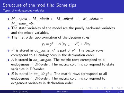
M_.npred + M_.nboth + M_.nfwrd + M_.static =M_.endo_nbrThe state variables of the model are the purely backward variablesand the mixed variables.The first order approximation of the decision rules

yt = y s + A (xt−1 − x s ) + Buty s is stored in oo_.dr.ys, x s is part of y s . The vector rowscorrespond to all endogenous in the declaration order.A is stored in oo_.dr.ghx. The matrix rows correspond to allendogenous in DR-order. The matrix columns correspond to statevariables in DR-order.B is stored in oo_.dr.ghu. The matrix rows correspond to allendogenous in DR-order. The matrix columns correspond toexogenous variables in declaration order.



Internally, Dynare uses two orderings of the endogenous variables:

the order of declaration (which is reflected in M_.endo_names)the order based on the four types described above, which we will callthe DR-order (“DR”stands for decision rules).

Most of the time, the declaration order is used, but for elements ofthe decision rules, the DR-order is used.

The DR-order is the following: static variables appear first, thenpurely backward variables, then mixed variables, and finally purelyforward variables. Inside each category, variables are arrangedaccording to the declaration order.

Variable oo_.dr.order_var maps DR-order to declaration order, forinstance, y s is stored in declearation order, theny s (oo_.dr .order_var) is tranformed to DR-order.



Variable oo_.dr.inv_order_var contains the inverse map, k-thdeclared variable is numbered oo_.dr.inv_order_var(k) in DR-order.


Excute the mod file in Matlab

addpath (’G:\program\ dynare\4.4.3\matlab’); //Add path of dynareto matlab,

pwd=’G:\My Program\Teaching\Bayesian DSGE\dynareslides\dynare code\Neoclassical’;cd (pwd) // set working directory

dynare *.mod


DSGE as State Space Model

DSGE model can be casted into a linear state space form

State equation

yt = Et [yt+1] + gt − Et [gt+1]−1τ

(Rt − Et [πt+1]− Et [zt+1]

)πt = βEt [πt+1] + κ

(yt −

τ

$gt

)yt = ct + gt

Rt = ρR Rt−1 + (1− ρR )ψ1πt + (1− ρR )ψ2

(yt −

τ

$gt

)where

κ =1− ν

νφπ2$, $ = τ + ϕ (1− α) +

α

1− α

gt = ρg gt−1 + εg ,t

zt = ρz zt−1 + εz ,t


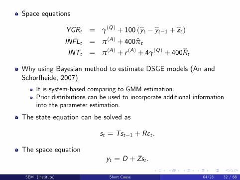
Space equations

YGRt = γ(Q ) + 100 (yt − yt−1 + zt )INFLt = π(A) + 400πt

INTt = π(A) + r (A) + 4γ(Q ) + 400Rt

Why using Bayesian method to estimate DSGE models (An andSchorfheide, 2007)

It is system-based comparing to GMM estimation.Prior distributions can be used to incorporate additional informationinto the parameter estimation.

The state equation can be solved as

st = Tst−1 + Rεt .

The space equationyt = D + Zst .


Bayesian Estimation for DSGE Model

Dejong, Ingram, and Whiteman (2000), Schorfheide (2000) and Otrok(2001) – the first papers using Bayesian techniques to DSGE models.

Smets and Wouters (2003, 2007) – more than a dozen hidden statesand 36 estimators.

Schorfheide (2000) and Otrok (2001) – Random Walk MetrolpolisHasting (RWMH) algorithm

95% of papers published from 2005 —2010 in eight top economicsjournals use the RWMH algorithm to estimate DSGE models (Herbst,2011)

Dynare with Matlab facilitates the use of the RWMH algorithm.


Bayesian Estimation for DSGE Model

Choosing prior density

Computing posterior mode

Simulating posterior distribution

Computing point estimates and confidence regions

Computing posterior probabilities


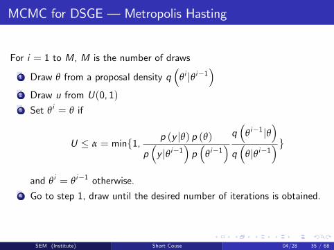
MCMC for DSGE – Metropolis Hasting

For i = 1 to M, M is the number of draws

1 Draw θ from a proposal density q(

θi |θi−1)

2 Draw u from U(0, 1)3 Set θi = θ if

U ≤ α = min{1, p (y |θ) p (θ)p(y |θi−1

)p(

θi−1) q(

θi−1|θ)

q(

θ|θi−1)}

and θi = θi−1 otherwise.4 Go to step 1, draw until the desired number of iterations is obtained.


Random Walk Metropolis Hasting

Random Walk Metropolis Hasting (RWMH) (Schorfheide, 2000):

θ = θi−1 + η, α = min{1, p (y |θ) p (θ)p(y |θi−1

)p(

θi−1)}

where η is a multivariate normal distribution with mean 0 andvariance cΣ.How to choose Σ

Σ−1 = −∂2 log p (θ|y)∂θ∂θ′

|θ=θm

where θm = argmax log p (θ|y).c is used to control the acceptance rate, 0.234 for multivariate normaltarget distribution (Roberts et al., 1997) and between 0.20− 0.40 inpractice.For the linearized case, p (y |θ) can be evaluated by Kalman Filter.SEM (Institute) Short Couse 04/28 36 / 68

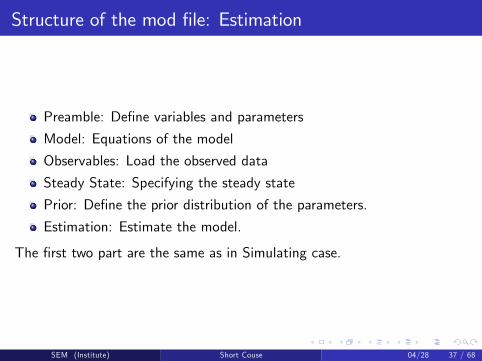
Structure of the mod file: Estimation

Preamble: Define variables and parameters

Model: Equations of the model

Observables: Load the observed data

Steady State: Specifying the steady state

Prior: Define the prior distribution of the parameters.

Estimation: Estimate the model.

The first two part are the same as in Simulating case.


Structure of the mod file: EstimationObservables and Prior

Observables: varobs y

Note that the number of the obsevations should be less than thenumber of shocks.

Prior: estimated_params;... end;

The four parameters: parameter name, prior shape, prior mean, priorstandard error


Structure of the mod file: EstimationPrior

The shape should be consistent with the domain of definition of theparameter

Use values obtained in other studies (micro or macro)

Check the graph of the priors

Check the implication of your priors by running stoch_simul withparameters set at prior mean

Do sensitivity tests by widening your priors


Structure of the mod file: EstimationSteady state

Give initial values for steady stateinitval;lc = -1.02;lk = -1.61;lz = 0;end;

Steady state must be calculated for many different values ofparameters, it is better to

Linearize the system yourself, then it is easy to solve for steady state.Give the exact solution of steady state as initial values.Provide program to calculate the steady state yourself.



Give the exact solution of steady state as initial values, in your *.modfile include:steady_state_model;lz = 0;lk = log(((1-beta*(1-delta))/(alpha*beta))^(1/(alpha-1)));lc = log(exp(lk)^alpha-delta*exp(lk));ly = alpha*lk;li = log(delta)+lk;end;

Provide program to calculate the steady state yourself.

If your *.mod file is called xxx.mod then write a filexxx_steadystate.m. The two files will be in the same directory.Dynare checks whether a file with this name exists and will use it.Sequence of output should correspond with sequence given in var list.



function [ys,check] = Neoclassical_estimation_ex_steadystate(ys,exo)global M_alpha = M_.params(1);beta = M_.params(2);delta = M_.params(3);rho = M_.params(4);nu = M_.params(5);z = 1;k = ((1-beta*(1-delta))/(alpha*beta))^(1/(alpha-1));c = k^alpha-delta*k;i = delta*k;y =c+i;ys =[ y; i; k; c; z ];ys =ln(ys);


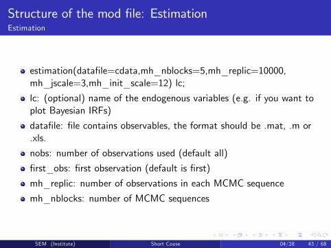
Structure of the mod file: EstimationEstimation

estimation(datafile=cdata,mh_nblocks=5,mh_replic=10000,mh_jscale=3,mh_init_scale=12) lc;

lc: (optional) name of the endogenous variables (e.g. if you want toplot Bayesian IRFs)

datafile: file contains observables, the format should be .mat, .m or.xls.

nobs: number of observations used (default all)

first_obs: first observation (default is first)

mh_replic: number of observations in each MCMC sequence

mh_nblocks: number of MCMC sequences


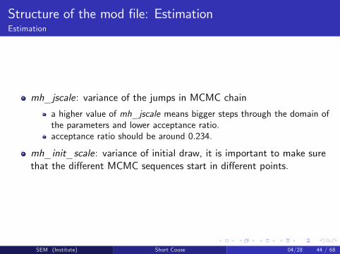
Structure of the mod file: EstimationEstimation

mh_jscale: variance of the jumps in MCMC chain

a higher value of mh_jscale means bigger steps through the domain ofthe parameters and lower acceptance ratio.acceptance ratio should be around 0.234.

mh_init_scale: variance of initial draw, it is important to make surethat the different MCMC sequences start in different points.


Result AnalysisConvergence

MCMC should generate sequence as if drawn from the posteriordistribution.

Minimum requirement is that distribution is same

for different parts of the same sequence.across sequence (if you have more than one).

θij the ith draw (out of I ) in the jth sequence (out of J), θj is themean of jth sequence,–θ is the mean across all available data (poolingall the data).

Define the between variance

BI=

1J − 1

J

∑j=1

(θj −–θ

)2where B

I is the estimator of the variance of sample mean.



Given a sequence {θi}Ii=1 which is i.i.d. from a random variable ywith variance σ2, the variance of the sample mean θ = ∑I

i=1 θi isσ2/I .If we have J different i.i.d. sequences from θ, which is denoted by{θij}Ii=1, then for each chain we have the mean θj , then {θj}Jj=1 is ani.i.d. sequence with variance σ2/I .BI is the estimator of σ2/I .



Define the within variance

W =1J

J

∑j=1

(1I

I

∑i=1

(θij − θj

)2),W =

1J

J

∑j=1

(1

I − 1I

∑i=1

(θij − θj

)2)

then W and W are both consistent estimators of σ2, since1I ∑I

i=1

(θij − θj

)2 is consistent estimator of σ2.

Between variance should go to zero, limI→∞BI −→ 0. And within

variance should settle down limI→∞ W −→ σ2.

In dynare, read line denote W as function of I and blue line denoteV = W + B

I

(1+ 1

m

).



We need red and blue line to get close, and red line to settle down.

The above can be done for any moment, not just the variance.

Dynare computes 3 sets of MCMC statistics

Interval: The length of the Highest Probability Density intervalcovering 80% of the posterior distribution.M2: VarianceM3: Skewness

For each of these, dynare computes a statistic related to thewithin-sequence value of each of these (red) and essentially a sum ofthe within-sequence statistic and a between-sequence variance (blue)



For each moment of interest you can calculate the multivariateversion, such as covariance matrix.

These higher-dimensional objects have to be transformed into scalarobjects that can be plotted.

The acceptance rate should be "around" 0.234.

A relatively low acceptance rate makes it more likely that the MCMCtravels through the whole domain of θ.If the acceptance rate is too high, you can increase mh_jscale.


Result AnalysisIRF

Impulse responses trace out the response of current and future valuesof each of the variables to a one-unit increase (or to a one-standarddeviation increase, when the scale matters) in the current value ofone of the VAR errors, assuming that this error returns to zero insubsequent periods and that all other errors are equal to zero.

The implied thought experiment of changing one error whileholding the others constant makes most sense when the errorsare uncorrelated across equations, so impulse responses aretypically calculated for recursive and structural VARs.


Result AnalysisIRF

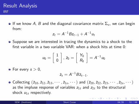
If we know A, B and the diagonal covariance matrix Σu , we can beginfrom:

zt = A−1Bzt−1 + A−1ut

Suppose we are interested in tracing the dynamics to a shock to thefirst variable in a two variable VAR: when a shock hits at time 0:

u0 =[10

], z0 =

[Y0R0

]= A−1u0

For every s > 0,zs = A−1Bzs−1.

Collecting (z10, z12, z13, · · · , z1s , · · · ) and (z20, z22, z23, · · · , z2s , · · · )as the impluse response of variables z1t and z2t to the structuralshock u1t respectively.


Result AnalysisIRF

The SVMA (structral vector moving average) representation of VAR is

zt = Φ (L) et = Φ0ut +Φ1ut−1 +Φ2ut−2 + · · ·+ · · ·

Consider the SVMA representation at time t + s[z1t+sz2t+s

]=

[φ11,0 φ12,0φ21,0 φ22,0

] [u1t+su2t+s

]+ · · ·

+

[φ11,s φ12,sφ21,s φ22,s

] [u1tu2t

]


Result AnalysisIRF

The structural dynamic multipliers are

∂z1t+su1t

= φ11,s ,∂z1t+su2t

= φ12,s

∂z2t+su1t

= φ21,s ,∂z2t+su2t

= φ22,s .

The structural impulse response functions (IRFs) are the plots of φij ,svs. s for i , j = 1, 2.

These plots summarize how unit impulses of the structural shocks attime t impact the level of z at time t + s for different values of s.


Result AnalysisIRF

In stoch_simul command, the option is irf = periods.

In estimation command, the option is bayesian_irf which is used totrigger the computation of IRFs. The length of the IRFs arecontrolled by the option irf = periods.


Result AnalysisForecast Error Variance Decomposition

Variance decomposition separates the variation in an endogenousvariable into the component shocks to the VAR.The variance decomposition provides information about the relativeimportance of each random innovation in affecting the variables in theVAR.The SVMA (structral vector moving average) representation of VAR is

zt = Φ (L) et = Φ0ut +Φ1ut−1 +Φ2ut−2 + · · ·+ · · ·

The error in forecasting zt in the future is, for each horizon s:

zt+s − Etzt+s = Φ0ut+s +Φ1ut+s−1 +Φ2ut+s−2 + · · ·+Φs−1ut+1

The variance of the forcasting error is

var (zt+s − Etzt+s ) = Φ0ΣuΦ′0+Φ1ΣuΦ′1+Φ2ΣuΦ′2+ . . .+Φs−1ΣuΦ′s−1(4)



Since Σu is diagonal, for the first equation

var (z1t+s − Etz1t+s ) = σ21 (s) = σ21(φ211,0 + φ211,1 + · · ·+ φ211,s−1

)+σ22

(φ212,0 + φ212,1 + · · ·+ φ212,s−1

),

And for the second

var (z2t+s − Etz2t+s ) = σ22 (s) = σ21(φ221,0 + φ221,1 + · · ·+ φ221,s−1

)+σ22

(φ222,0 + φ222,1 + · · ·+ φ222,s−1

).

The proportion of σ21 (s) due to shocks in u1t is then

ρ1,1 =σ21(φ211,0 + φ211,1 + · · ·+ φ211,s−1

)σ21 (s)

,



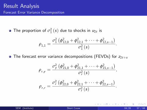
The proportion of σ21 (s) due to shocks in u2t is

ρ1,1 =σ21(φ212,0 + φ212,1 + · · ·+ φ212,s−1

)σ21 (s)

.

The forecast error variance decompositions (FEVDs) for z2t+s

ρr ,y =σ2y(φ221,0 + φ221,1 + · · ·+ φ221,s−1

)σ2r (s)

,

ρr ,r =σ2r(φ222,0 + φ222,1 + · · ·+ φ222,s−1

)σ2r (s)

.


Result AnalysisForecast Error Variance Decomposition (FEVD)

conditional_variance_decomposition = INTEGER

conditional_variance_decomposition = [INTEGER1:INTEGER2]

conditional_variance_decomposition = [INTEGER1 INTEGER2 ...]

In stoch_simul comand, the conditional variance decomposition iscomputed at calibrated values of parameters.

In estimation comand, these options compute the posteriordistribution of the conditional variance decomposition, for thespecified period(s).

Note that this option requires the option moments_varendo to bespecified.


Result AnalysisModel Comparison

Prior density p (θA |A), where A represents the model and θA, theparameters of that model.

Conditional densityp (y |θA,A)

Conditional density for dynamic time series models

p (YT |θA,A) = p (y0|θA,A)T

∏t=1p (yt |YT−1, θA,A)

where YT are the observations until period T .

Likelihood function

L (θA |YT ,A) = p (YT |θA,A)



Geweke (1999) modified harmonic mean

P (YT |A) =∫

ΘA


P (YT |A) =

1n

n

∑i=1

f(

θ(i )A

)p(YT |θ(i )A ,A

)p(

θ(i )A |A

)−1

where

f (θ) = p−1 (2π)−k/2∣∣∣ΣθMA

∣∣∣−1/2exp

{−12

(θ − θMA

)Σ−1

θMA

(θ − θMA

)′}×{(

θ − θMA

)Σ−1

θMA

(θ − θMA

)′≤ F−1X 2k (p)

}with p an arbitray probability and k, the number of eatimatedparameters.



ΣθMAis the minus second order derivative of p (YT |θA,A) p (θA |A)

evaluated at the mode θMA .

Larger marginal likelihood means a better model.

In Geweke (1999) modified harmonic mean, f (θ) is truncatedmultivariate normal distribution.

In Geweke (1999) modified harmonic mean, we need to use theposterior draws and the mode.

For Laplace method, we only need the mode.



In Dynare, the marginal density can be compute by estimationcommand.

The Laplace approximation of marginal density is stored inoo._MarginalDensity.LaplaceApproximation.

The Modified Harmonic Mean of marginal density is stored inoo._MarginalDensity.ModifiedHarmonicMean which is used withmh_replic>0 or load_mh_file option.


Result AnalysisLoop with dynare

Sometimes we need to include dynare in a loop of matlab overdifferent parameters.

In our AR(1) model, starting with .m file with the following code:rho = 0.90;se = 0.01;save parameterfile rho se

And in the .mod file, we change the code toparameters rho,se; // Parameters of the modelload parameterfileset_param_value(’rho’, rho);set_param_value(’se’, se);


Result AnalysisLoop with dynare

To include dynare in a loop of Matlab, we use the following coderho_value=[0.85 0.90 0.95];N = size(rho_value,2);se = 0.01;Simmean=zeros(N,1); % We want to get the simulated mean foreach value of rhofor i=1:Nrho = rho_value(i);save parameterfile rho sedynare AR_demo.mod noclearallSimmean(i)=oo_.mean;end


simulating and estimating dsge model with dynare›¾涛-dyanre-slides.pdf · simulating and...

Documents