simulated turbulent fluxes over land from general circulation models and reanalyses compared with...

INTERNATIONAL JOURNAL OF CLIMATOLOGY

Int. J. Climatol. 22: 1235–1247 (2002)

Published online 24 May 2002 in Wiley InterScience (www.interscience.wiley.com). DOI: 10.1002/joc.792

SIMULATED TURBULENT FLUXES OVER LAND FROM GENERALCIRCULATION MODELS AND REANALYSES COMPARED WITH

OBSERVATIONS

R. SHEPPARD* and M. WILDInstitute for Atmospheric and Climate Sciences, ETH, Winterthurerstrasse 190, Zurich 8057, Switzerland

Received 28 February 2001Revised 20 February 2002

Accepted 3 March 2002

ABSTRACT

Turbulent fluxes over land in three general circulation models (GCMs) and the three reanalyses are compared with long-term measurements. Observations were obtained from a variety of sources, including GEBA, Cabauw, The Netherlands,and two newly analysed sites. The intercomparison reveals a wide range of values between the models. The latent heatflux in two of the models shows good agreement with observations. These models benefit from accurately simulatedradiative fluxes. The other models tend to overestimate the latent heat flux as long as there is sufficient soil moistureavailable. This overestimation is caused by a variety of reasons, including: a too intense zonal flow from the ocean to theinterior of the continent, which produces an excessive moist advection, thereby increasing precipitation and evaporation;and a high insolation and soil moisture, producing excessive latent heat flux in summer. Where soil moisture is limitedtoo early, an excessive decrease in latent heat flux is apparent towards the end of summer. The sensible heat flux in themodels varies when compared with the observations due to the following possibilities: in models that exhibit an excessivesummer drying, too much available energy will be partitioned into the sensible heat flux at the end of summer, since thereis no water available for evaporation; in models where radiation is overestimated, the excessive available energy willlead to an overestimated sensible heat flux. Despite the continuous assimilation of observations from the global observingsystem in the reanalyses, the range of uncertainties is not reduced when compared with the GCMs. Thus, although thereanalysis project was developed to aid the validation of GCMs, it appears to be difficult to accomplish this in the caseof the turbulent fluxes. Copyright 2002 Royal Meteorological Society.

KEY WORDS: turbulent fluxes; general circulation models; latent heat; sensible heat; reanalyses.

1. INTRODUCTION

Turbulent fluxes over land form a direct link between the energy and water balance. The latent heat fluxbetween the surface and atmosphere determines the humidity, and the sensible heat flux largely governsthe temperature in the lowest layers. The relative importance of sensible versus latent heat flux is mainlydetermined by the availability of water for evaporation, although the available atmospheric heat and watervapour sinks are also important. However, although the turbulent fluxes over land are key variables in theclimate system, their validation in general circulation models (GCMs) has largely been ignored. Garratt (1993)made a comparison between different models over Amazonia, and Beljaars and Viterbo (1994) completeda similar study for Cabauw, The Netherlands. Garratt et al. (1993) compared the energy balance over fivecontinents with GCMs using the maps of Henning (1989). More recently, large-scale projects such as FIFE(First International Satellite Land Surface Climatology Project (ISLSCP) Field Experiment; Sellers et al.,1992) have been completed. However, the major drawback of these campaigns is the short time period atwhich the fluxes are measured. Additionally, large-scale projects such as the Project for the Intercomparison

* Correspondence to: R. Sheppard, Institute for Atmospheric and Climate Sciences, ETH, Winterthurerstrasse 190, Zurich 8057,Switzerland; e-mail: [email protected]

Copyright 2002 Royal Meteorological Society

1236 R. SHEPPARD AND M. WILD

of Landsurface Parameterization Schemes (PILPS) compare GCM results to the reanalyses (e.g. PILPS 2000PCMDI report, http://www-pcmdi.llnl.gov/pilps3/). The difficulty, however, with using the reanalyses is thatthese data are also model generated. This has the disadvantage over direct observations that errors in therespective analysis models will propagate to the reanalyses. Lastly, Wild et al. (1996) used direct observationsof evaporation at a number of sites in Europe to validate the ECHAM GCM from the Max-Planck Institute forMeteorology (MPI), Hamburg. This paper will extend the work of Wild et al. (1996) in two ways. Firstly, bothobservational sensible and latent heat fluxes will be used (compared with only latent heat flux in Wild et al.(1996)); secondly, three GCMs and the three reanalysis models will be analysed, pointing out the differencesbetween the models and direct observations on a local scale.

This paper will be set out as follows. In Section 2, the models used will be presented; this is followed by ashort description of the observational sites in Section 3. Section 4 will discuss the shortcomings in the modelswhen compared with observations. The emphasis will be on the summer season. Finally, the conclusions willbe presented in Section 5.

2. MODEL DESCRIPTION

The models used in this study are: the ECHAM4 GCM from the Max-Planck Institute for Meteorology (hence-forth ECHAM4), Hamburg (Roeckner et al., 1996); the HadAM2b GCM from the Hadley Centre for ClimatePrediction and Research (henceforth HadAM2b), Bracknell, UK (Stratton, 1999); and the ARPEGE GCM fromMeteo-France (henceforth ARPEGE), Toulouse (Deque et al., 1994). Additionally, three reanalysis modelswere used. They are: the European Centre for Medium-Range Weather Forecasts (henceforth ERA) reanalysismodel, Reading, UK (Gibson et al., 1997); the National Centers for Environmental Prediction–National Cen-ter for Atmospheric Research (henceforth NCEP) reanalysis model, Washington, US (Kalnay et al., 1996);and the NASA/Data Assimilation Office (henceforth GEOS) reanalysis model (Schubert et al., 1993).

The reanalysis systems include fixed versions of an operational data assimilation and modelling system toreanalyse historical data. These multiyear simulations have been completed to provide a physically consistentdataset of the atmosphere that is believed to be useful for validation purposes.

The GCMs used in this study were integrated over periods of 10 years and use prescribed sea surfacetemperatures (SSTs) and sea ice for the period 1979–88 according to the Atmospheric Model IntercomparisonProject (AMIP; Gates, 1992). On the other hand, the reanalysis data were integrated over varying periods.The periods available for this study were: 1985–93 for ERA; 1982–94 for NCEP; and 1981–92 for GEOS.

The GCM experiments analysed in this study were performed at a high resolution (T106, which correspondsto 1.1° × 1.1°), while the reanalyses correspond to varying horizontal resolutions. Namely: T106 for ERA;T62 (2.5° × 2.5°) for NCEP; and 2° × 2.5° for GEOS.

The determination of the turbulent fluxes varies with each model, and will be discussed below.All the models calculate the turbulent fluxes at the surface according to the bulk transfer relation:

(w′χ ′)s = −Cχ |vL|(χL − χs) (1)

where χ is the turbulent flux variable (temperature or specific humidity), w′ is the fluctuation in vertical windspeed, Cχ is the transfer coefficient, vL is the horizontal wind vector at L, where L is the lowest model level(representing the top of the surface layer), and s signifies surface.

The transfer coefficients in ECHAM4 are obtained from Monin–Obukhov similarity theory by integratingthe flux–profile relationships over the lowest model layer and are based on Louis (1979). For evaporation,it is assumed that relative humidity at the surface is a function of the water content of the soil. Further,evaporation over vegetation is proportional to the evaporation efficiency, which is determined from thestomatal resistance of the canopy. The stomatal resistance is determined from the available water in the rootzone, the photosynthetically active radiation (PAR) and the leaf area index (LAI). For more information, seeWild et al. (1996) and Roeckner et al. (1996).

In HadAM2b, the transfer coefficients are obtained from Monin–Obukhov similarity theory using theformulations in Smith (1996). For evaporation, when the specific humidity at the lowest model level is greater

Copyright 2002 Royal Meteorological Society Int. J. Climatol. 22: 1235–1247 (2002)

TURBULENT FLUXES OVER LAND 1237

than that at the surface, the surface specific humidity is set to zero. On the other hand, for land surfaces witha positive moisture flux, the resistance method of Monteith (1965) is used to calculate evaporation, wherebythe physiological control of water loss through the vegetation is characterized by the stomatal resistance.Here, the stomatal resistance is a climatologically prescribed, geographically varying quantity dependent onthe vegetation type only (Smith, 1996).

As with ECHAM4, the transfer coefficients in ARPEGE are those proposed by Louis (1979) and arefunctions of the roughness length and Richardson number. Evaporation is assumed to take place at a potentialrate over bare soil when the soil moisture is larger than the field capacity. As with ECHAM4, stomatalresistance is determined from the available water in the root zone, the PAR and the LAI. In addition, thestomatal resistance is also dependent on the effects of the vapour pressure deficit of the atmosphere and onthe dependence of air temperature on the surface resistance (Noilhan and Planton, 1989).

In ERA, the transfer coefficients between the surface (skin) and the lowest model level are not expressed asfunctions of the bulk Richardson number as in Louis (1979), but are expressed as a function of the Obukhovlength (Beljaars and Viterbo, 1994). For evaporation, it is assumed that the relative humidity depends on thesoil wetness of the top layer. As with ECHAM4, the computation of the stomatal resistance depends on thePAR, LAI and the soil wetness in the root zone. The stomatal resistance is based on an integration across thecanopy of the conductances of individual horizontal leaves acting in parallel (Viterbo and Beljaars, 1995).

The transfer coefficients in NCEP are also based on the formulations of Louis (1979) using Monin–Obukhovsimilarity theory. The evaporation in NCEP is related to the soil moisture deficit and the plant resistance totranspiration, as discussed in Monteith (1981). The computation of potential evaporation (which is required todetermine the actual evaporation) follows the Penman method (Marht and Ek, 1984) with increased numericalefficiency and the addition of upward longwave radiation depending on temperature (Troen and Mahrt, 1986).As with the other models, the NCEP reanalysis does not distinguish between the surface air temperature at thelevel of the roughness elements as used in surface-layer similarity theory and the effective surface radiationtemperature.

The transfer coefficients in GEOS are obtained from Monin–Obukhov similarity theory by selectingsimilarity functions that approach the convective limit for unstable profiles (Panofsky, 1973) and that agreewith observations for very stable profiles (Clarke, 1970). GEOS does not have a coupled land surface modeland requires soil moisture to be specified. The determination of the soil moisture climatology is based onThornthwaite (1948) and Mintz and Serafini (1992), and does not account for frozen ground or ice formation.The potential evapotranspiration (which is required to determine the actual evapotranspiration) is estimatedas a function of monthly mean air temperature and the duration of daylight (Schemm et al., 1992).

3. OBSERVATIONAL DATA

The turbulent fluxes used in this study have been extracted from the Global Energy Balance Archive (GEBA;Gilgen et al., 1997) database at the authors’ institute, as well as from other sources. The sites for the sensibleheat flux are generally different than those for the latent heat flux, since there are only limited long-termentries of sensible heat flux available in GEBA. The sites for the latent and sensible heat flux will be discussedseparately in the following section.

3.1. Latent heat flux observational sites

Evaporation can be determined by a number of methods, including the eddy correlation method, lysimetermeasurements, the profile method and Bowen ratio method (Brutsaert, 1982). However, though fieldcampaign measurements over short durations are abundant, long-term measurements (which allow estimatesof climatologies) are relatively few. For this study, only those sites with more than three continuous yearsof measurements were used, thereby reducing the spurious extremes possible on shorter time scales andincreasing the representativity of the sites. The six sites used here are: Cabauw, The Netherlands (Beljaars andViterbo, 1994); Dunedin, New Zealand (Fahey et al., 1996); Tsukuba, Japan (Kotoda, 1984); Basel–Binningen,



Switzerland (Schuepp, 1983); Hartheim, Germany (Jaeger and Kessler, 1997); and Rietholzbach, Switzerland(Menzel, 1991).

Measurements from Cabauw, The Netherlands (51°58′N, 4°56′E, −0.5 m a.s.l.) are obtained for the years1987–96 using the profile method. A complete overview of this site can be found in van Ulden and Wieringa(1996).

A newly analysed site at Dunedin, New Zealand (45°47′S, 170°29′E, 710 m a.s.l.) was used in this study.The site lies on a north–south-oriented plateau covered with tussock grass. The regional climate is quitesevere, with prevailing westerly winds, intense rain and the possibility of snow in any month. Measurementsof evaporation were taken from 1991–96 using a weighing lysimeter. The lysimeter weight changes aredetected as pulses from a reversible screw that drives a travelling weight along the lever arm to maintainthe balance (Fahey et al., 1996). Excess water drains from the monolith base and is measured by a tippingbucket. Additionally, measurements of precipitation are taken from up to eight tipping bucket gauges. Thus,evaporation is calculated from the water balance equation:

E = �S − P − Q (2)

where E is the evaporation, �S is the change in weight storage calculated from the lysimeter weight change,P is the precipitation, and Q is the drainage from the base of the lysimeter.

The site at Tsukuba, Japan (36°7′N, 140°6′E, 27 m a.s.l.) was also newly analysed for this study.Measurements of evaporation were taken from a weighing lysimeter for the period 1981–97 (Niimura, personalcommunication).

The sites from Basel–Binningen, Switzerland (47°35′N, 7°35′E, 317 m a.s.l.), Hartheim, Germany (47°56′N,7°37′E, 201 m a.s.l.) and Rietholzbach, Switzerland (47°23′N, 9°E, 760 m a.s.l.) were obtained from the GEBAdatabase (Gilgen et al., 1997). Measurements in Basel–Binningen (1977–86) and Rietholzbach (1977–84)both used weighing lysimeters, whereas Hartheim (1974–91) used the water balance equation (Equation (2)).

3.2. Sensible heat flux observational sites

Relatively few long-term measurements are available for the sensible heat flux. As such, sites with morethan 12 months of continuous measurements were used. The sensible heat flux is typically derived from theresidual of the energy balance. The six sites used in this study include: Cabauw, The Netherlands (Beljaars andViterbo, 1994); Tumengalha, Tibet (Liu and Zeng, 1965); Tsukuba, Japan (Niimura, personal communication);Copenhagen, Denmark (Aslyng and Nielson, 1961); Hartheim, Germany (Jaeger and Kessler, 1997); andBarrow, Alaska (Maykut and Church, 1973). The main difference with the Hartheim site is that the sensibleheat flux is determined above a pine forest.

Measurements of sensible heat flux at the Cabauw site are derived from the residual of the energy balance(Equation (3)) for the period 1987–96:

H = Rn − G − LE (3)

where H is the sensible heat flux, Rn is the net radiation, G is the soil heat flux, and LE is the latent heatflux. Further details can be found in van Ulden and Wieringa (1996).

For Tsukuba, Japan, the sensible heat flux was determined using sonic anemometer–thermometers at 1.6 mabove the surface for the period 1981–97 (Niimura, personal communication).

For Tumengalha, Tibet (32°51′N, 90°18′E, 3841 m a.s.l.), Copenhagen, Denmark (55°40′N, 12°18′E, 28 ma.s.l.), Hartheim, Germany (47°56′N, 7°37′E, 201 m a.s.l.) and Barrow, Alaska (71°11′N, 203°20′E, 10 ma.s.l.), the sensible heat fluxes were derived by calculating the residual of the energy balance (see Equation (3))for 12 months, 3 years, 12 years and 15 years respectively.

Long-term measurements of net radiation were also available for this study for the sites at Cabauw, TheNetherlands, Hartheim, Germany, and Tsukuba, Japan.



4. RESULTS

To compare the models with point observations, up to four surrounding land points were area-weighted toprovide the simulated turbulent flux for the exact location. Ocean grid points were excluded for this study.The representativeness of area-weighted grid points has been successfully researched at both Cabauw, TheNetherlands (Beljaars et al., 1983; Beljaars and Bosveld, 1997; Beljaars and Holtslag, 1991), and Rietholzbach,Switzerland (Furholz, 1994; Wild et al., 1996). Although no such studies have been completed for theremaining sites, the orography and albedo present at each measurement site are comparable to that found inthe area-weighted grid point used in this study, thus increasing the suitability of each site.

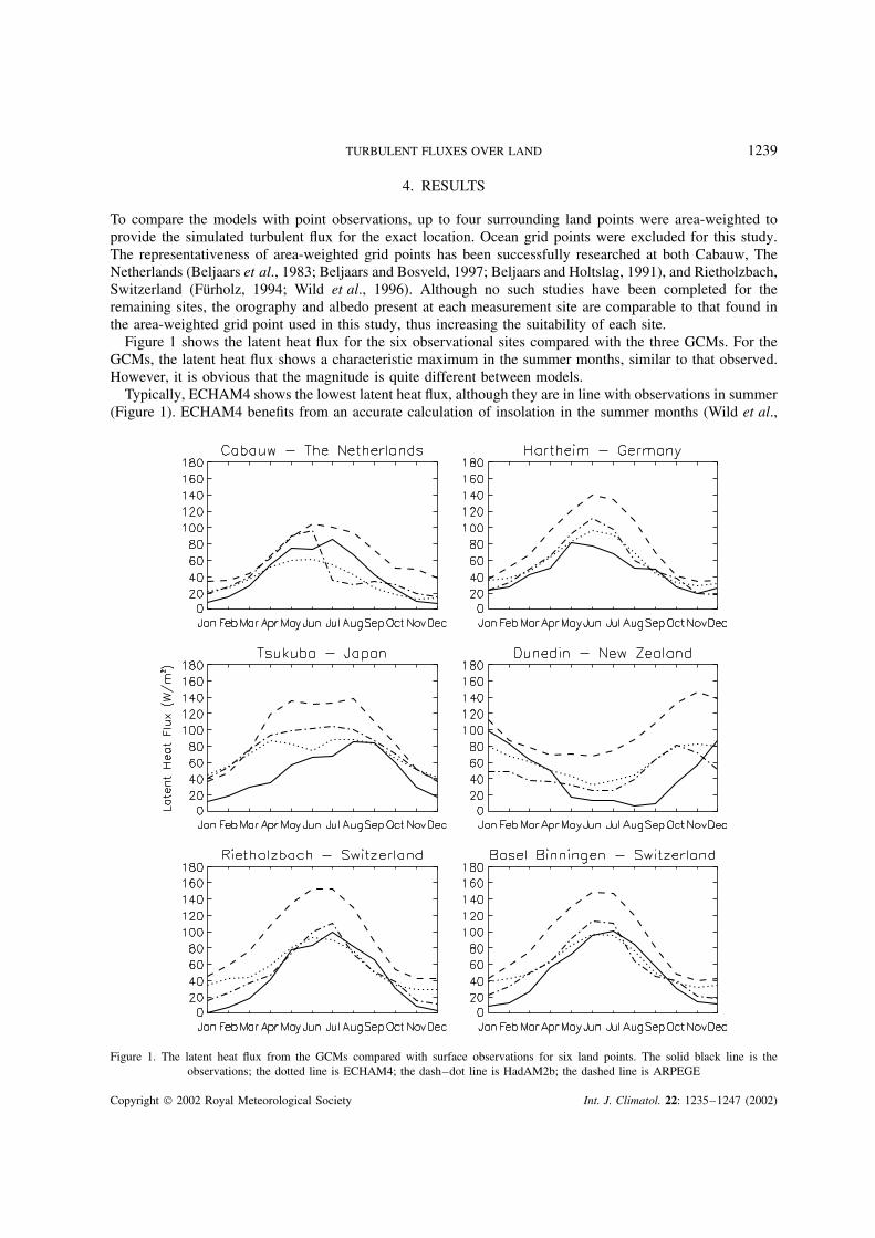
Figure 1 shows the latent heat flux for the six observational sites compared with the three GCMs. For theGCMs, the latent heat flux shows a characteristic maximum in the summer months, similar to that observed.However, it is obvious that the magnitude is quite different between models.

Typically, ECHAM4 shows the lowest latent heat flux, although they are in line with observations in summer(Figure 1). ECHAM4 benefits from an accurate calculation of insolation in the summer months (Wild et al.,

Figure 1. The latent heat flux from the GCMs compared with surface observations for six land points. The solid black line is theobservations; the dotted line is ECHAM4; the dash–dot line is HadAM2b; the dashed line is ARPEGE



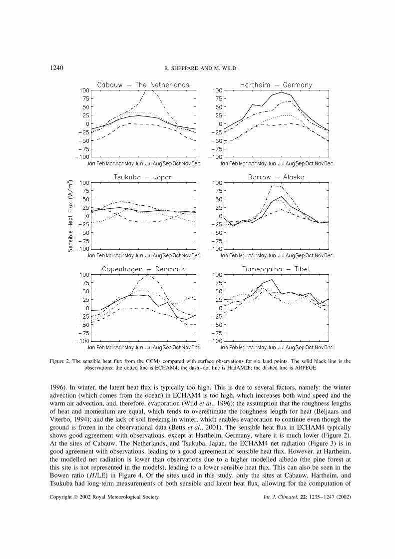
Figure 2. The sensible heat flux from the GCMs compared with surface observations for six land points. The solid black line is theobservations; the dotted line is ECHAM4; the dash–dot line is HadAM2b; the dashed line is ARPEGE

1996). In winter, the latent heat flux is typically too high. This is due to several factors, namely: the winteradvection (which comes from the ocean) in ECHAM4 is too high, which increases both wind speed and thewarm air advection, and, therefore, evaporation (Wild et al., 1996); the assumption that the roughness lengthsof heat and momentum are equal, which tends to overestimate the roughness length for heat (Beljaars andViterbo, 1994); and the lack of soil freezing in winter, which enables evaporation to continue even though theground is frozen in the observational data (Betts et al., 2001). The sensible heat flux in ECHAM4 typicallyshows good agreement with observations, except at Hartheim, Germany, where it is much lower (Figure 2).At the sites of Cabauw, The Netherlands, and Tsukuba, Japan, the ECHAM4 net radiation (Figure 3) is ingood agreement with observations, leading to a good agreement of sensible heat flux. However, at Hartheim,the modelled net radiation is lower than observations due to a higher modelled albedo (the pine forest atthis site is not represented in the models), leading to a lower sensible heat flux. This can also be seen in theBowen ratio (H /LE) in Figure 4. Of the sites used in this study, only the sites at Cabauw, Hartheim, andTsukuba had long-term measurements of both sensible and latent heat flux, allowing for the computation of



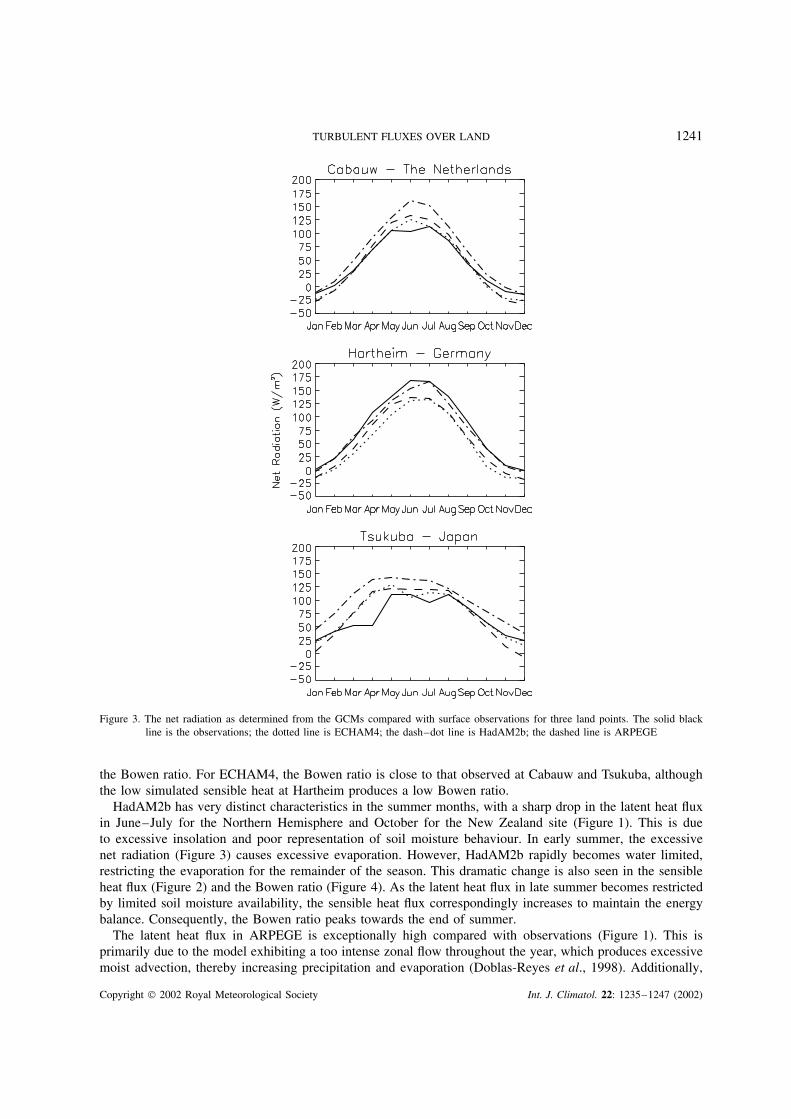
Figure 3. The net radiation as determined from the GCMs compared with surface observations for three land points. The solid blackline is the observations; the dotted line is ECHAM4; the dash–dot line is HadAM2b; the dashed line is ARPEGE

the Bowen ratio. For ECHAM4, the Bowen ratio is close to that observed at Cabauw and Tsukuba, althoughthe low simulated sensible heat at Hartheim produces a low Bowen ratio.

HadAM2b has very distinct characteristics in the summer months, with a sharp drop in the latent heat fluxin June–July for the Northern Hemisphere and October for the New Zealand site (Figure 1). This is dueto excessive insolation and poor representation of soil moisture behaviour. In early summer, the excessivenet radiation (Figure 3) causes excessive evaporation. However, HadAM2b rapidly becomes water limited,restricting the evaporation for the remainder of the season. This dramatic change is also seen in the sensibleheat flux (Figure 2) and the Bowen ratio (Figure 4). As the latent heat flux in late summer becomes restrictedby limited soil moisture availability, the sensible heat flux correspondingly increases to maintain the energybalance. Consequently, the Bowen ratio peaks towards the end of summer.

The latent heat flux in ARPEGE is exceptionally high compared with observations (Figure 1). This isprimarily due to the model exhibiting a too intense zonal flow throughout the year, which produces excessivemoist advection, thereby increasing precipitation and evaporation (Doblas-Reyes et al., 1998). Additionally,



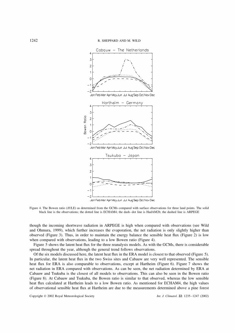
Figure 4. The Bowen ratio (H /LE) as determined from the GCMs compared with surface observations for three land points. The solidblack line is the observations; the dotted line is ECHAM4; the dash–dot line is HadAM2b; the dashed line is ARPEGE

though the incoming shortwave radiation in ARPEGE is high when compared with observations (see Wildand Ohmura, 1999), which further increases the evaporation, the net radiation is only slightly higher thanobserved (Figure 3). Thus, in order to maintain the energy balance the sensible heat flux (Figure 2) is lowwhen compared with observations, leading to a low Bowen ratio (Figure 4).

Figure 5 shows the latent heat flux for the three reanalysis models. As with the GCMs, there is considerablespread throughout the year, although the general trend follows observations.

Of the six models discussed here, the latent heat flux in the ERA model is closest to that observed (Figure 5).In particular, the latent heat flux in the two Swiss sites and Cabauw are very well represented. The sensibleheat flux for ERA is also comparable to observations, except at Hartheim (Figure 6). Figure 7 shows thenet radiation in ERA compared with observations. As can be seen, the net radiation determined by ERA atCabauw and Tsukuba is the closest of all models to observations. This can also be seen in the Bowen ratio(Figure 8). At Cabauw and Tsukuba, the Bowen ratio is similar to that observed, whereas the low sensibleheat flux calculated at Hartheim leads to a low Bowen ratio. As mentioned for ECHAM4, the high valuesof observational sensible heat flux at Hartheim are due to the measurements determined above a pine forest



Figure 5. As for Figure 1, but for the reanalyses. The solid black line is the observations; the dotted line is ERA; the dashed line isNCEP; the dash–dot line is GEOS

as opposed to surface measurements. However, the area-weighted grid point was still deemed to be the mostrepresentative of the site, and was therefore used in this study.

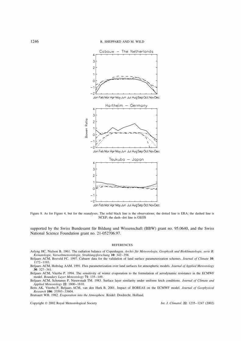
The latent heat flux in NCEP is typically higher than observations (Figure 5). A major factor contributing tothis is an excessive incoming radiation, which increases the evaporation. This can also be seen in the excessivenet radiation in NCEP (Figure 7). Contrary to HadAM2b, NCEP has sufficient soil moisture throughout theyear (not shown). Thus, the high radiation leads to high evaporation. The sensible heat flux in NCEP differsfrom observations, with values slightly lower than observed at some sites (Barrow and Hartheim) and slightlyhigher than observed at others (Cabauw and Copenhagen) (Figure 6). Therefore, the Bowen ratio is quitesimilar to observations (Figure 8). However, since the sensible heat flux at Hartheim is low, the Bowen ratiois also lower than observed.

Lastly, the latent heat flux in GEOS is exceptionally high when compared with observations (Figure 5).This is due largely to exceptionally high incoming radiation and a large soil moisture availability. Thus,GEOS is never water limited. The sensible heat flux is also quite high (Figure 6). Since the net radiationis exceptionally high (Figure 7) in GEOS, there is ample energy available to partition into both latent and




sensible heat fluxes, leading to high values in both the turbulent fluxes. As both sensible and latent heat fluxesare too high, the Bowen ratio appears comparable to observations, except at Hartheim, as discussed above(Figure 8).

5. CONCLUSIONS

The turbulent fluxes over land are known to be important determinants of the hydrological cycle and energybalance. However, their validation in GCMs and reanalyses have largely been ignored. Therefore, this studyattempts to discern the difficulties in parameterizing these fields. This is achieved by comparing the turbulentfluxes in the models with long-term measurements from various observational sites.

Typically, the GCMs and reanalyses show large differences in the turbulent fluxes. Despite the constraintsdue to assimilated observational atmospheric data, the reanalyses still show a surprisingly large range ofvalues for the turbulent fluxes. Thus, it is difficult to ascertain the accuracy of using these models in thevalidation of GCMs.




Results indicate that the turbulent fluxes in ERA and ECHAM4 are the closest to those observed. Thisis largely due to an accurate parameterization of radiation in these models (Wild et al., 1996). On the otherhand, the turbulent fluxes in HadAM2b, ARPEGE, NCEP and GEOS show larger biases compared withobservations. This is for a variety of reasons: an excessive summer drying in HadAM2b; a too intense zonalflow producing excessive moist advection in ARPEGE; and exceptionally high incoming radiation in NCEPand GEOS. Thus, although substantial progress has been made in the parameterization of the turbulent fluxes,it appears that there is still little consensus between modelling groups.

ACKNOWLEDGEMENTS

We are indebted to the members of MPI, Meteo-France, the Hadley Centre for Climate Research, the ECMWF,NCEP–NCAR and NASA who made the necessary model datasets available for this study. We would alsolike to thank Dr David Murray (University of Otago), Dr Fred Bosveld (KNMI), Dr Noriko Niimura (TERC)and Dr Hans Gilgen (ETH), who provided the observational data for this study. Special thanks should alsogo to Professor Atsumu Ohmura (ETH). This study evolved from the EU project HIRETYCS and has been




supported by the Swiss Bundesamt fur Bildung und Wissenschaft (BBW) grant no. 95.0640, and the SwissNational Science Foundation grant no. 21-052706.97.

REFERENCES

Aslyng HC, Nielson B. 1961. The radiation balance of Copenhagen. Archiv fur Meteorologie, Geophysik und Bioklimatologie, serie B:Keinatologie, Varweltmeteorologie, Strahlungsforschung 10: 342–358.

Beljaars ACM, Bosveld FC. 1997. Cabauw data for the validation of land surface parameterization schemes. Journal of Climate 10:1172–1193.

Beljaars ACM, Holtslag AAM. 1991. Flux parameterization over land surfaces for atmospheric models. Journal of Applied Meteorology30: 327–341.

Beljaars ACM, Viterbo P. 1994. The sensitivity of winter evaporation to the formulation of aerodynamic resistance in the ECMWFmodel. Boundary Layer Meteorology 71: 135–149.

Beljaars ACM, Schotanus P, Nieuwstadt TM. 1983. Surface layer similarity under uniform fetch conditions. Journal of Climate andApplied Meteorology 22: 1800–1810.

Betts AK, Viterbo P, Beljaars ACM, van den Hurk B. 2001. Impact of BOREAS on the ECMWF model. Journal of GeophysicalResearch 106: 33593–33604.

Brutsaert WH. 1982. Evaporation into the Atmosphere. Reidel: Dordrecht, Holland.



Clarke RH. 1970. Observational studies in the atmospheric boundary layer. Quarterly Journal of the Royal Meteorological Society 96:91–114.

Deque M, Dreveton C, Braun A, Cariolle D. 1994. The ARPEGE/IFS atmospheric model: a contribution to the French communityclimate modelling. Climate Dynamics 10: 249–266.

Doblas-Reyes FJ, Deque M, Braun A, Piedelievre JPh. 1998. Impact of resolution on variability in the CNRM runs: task C1. InProceedings of the 3rd HIRETYCS Meeting, Bologna, Italy; 17–19.

Fahey BD, Murray DL, Jackson RM. 1996. Detecting fog deposition to tussock by lysimetry at Swampy Summit near Dunedin, NewZealand. Journal of Hydrology 35: 87–104.

Furholz B. 1994. Die Berechnung der Wasserhaushaltsbilanz an einem voralpinen Einzugsgebiet mit einem Wasserhaushaltsmodell.Diploma Thesis, Institute for Geography, ETH, Zurich.

Garratt JR. 1993. Sensitivity of climate simulations to land-surface and atmospheric boundary-layer treatments — a review. Journal ofClimate 6: 419–449.

Garratt JR, Krummel PB, Kowalczyk EA. 1993. The surface energy balance at local and regional scales — a comparison of generalcirculation model results with observations. Journal of Climate 6: 1090–1109.

Gates WL. 1992. AMIP: the Atmospheric Model Intercomparison Project. Bulletin of the American Meteorological Society 73:1962–1970.

Gibson JK, Kallberg P, Uppala S, Hernandez A, Nomura A, Serrano E. 1997. ERA description. ECMWF reanalysis Project ReportSeries, 1, Reading.

Gilgen H, Wild M, Ohmura A. 1997. Global Energy Balance Archive GEBA — Report 3: The GEBA Version 1997 Database. WorldClimate Program — Water. Project A7. Zurcher Geographisches Schriften 74.

Henning D. 1989. Atlas of the Surface Heat Balance of the Continents. Gebruder Borntraeger: 402 pp.Jaeger L, Kessler A. 1997. Twenty years of heat and water balance climatology at the Hartheim pine forest, Germany. Agricultural and

Forest Meteorology 84: 25–36.Kalnay E, Kanamitsu M, Kistler R, Collins W, Deaven D, Gandin L, Iredell M, Saha S, White G, Woollen J, Zhu Y, Chelliah M,

Ebisuzaki W, Higgins W, Janowiak J, Mo KC, Ropelewski C, Wang J, Leetmaa A, Reynolds R, Jenne R, Joseph D. 1996. The NCEP/NCAR 40-year reanalysis project. Bulletin of the American Meteorological Society 77: 437–471.

Kotoda K. 1984. Heat balance and evapotranspiration of a grassland. Geographical Review of Japan A 57: 611–627.Liu G, Zeng X. 1965. Some Characteristics of Radiation Balance on Glacier No. 1 During the Ablation Season in Headwater of Urumqui

River, Tianshan. Science Press: Beijing; 54–62.Louis JF. 1979. A parametric model of vertical eddy fluxes in the atmosphere. Boundary Layer Meteorology 17: 187–202.Mahrt L, Ek M. 1984. The influence of atmospheric stability on potential evaporation. Journal of Climatology and Applied Meteorology

23: 222–234.Maykut G, Church PE. 1973. Radiation climate at Barrow, Alaska, 1962–66. Journal of Applied Meteorology 12: 620–628.Menzel L. 1991. Wasserhaushaltsstudien im Einzugsgebiet der Thur (Ostschweiz). Berichte und Skripten Nr. 46.Mintz Y, Serafini Y. 1992. A global monthly climatology of soil moisture and water balance. Climate Dynamics 8: 13–27.Monteith JL. 1965. Evaporation and environment. Symporia for the Society for Experimental Biology 19: 205–234.Monteith JL. 1981. Presidential address: evaporation and surface temperature. Quarterly Journal of the Royal Meteorological Society

107: 1–24.Noilhan J, Planton S. 1989. A simple parameterization of land surface processes for meteorological models. Monthly Weather Review

117: 536–549.Panofsky HA. 1973. Tower micrometeorology. In Workshop on Micrometeorology. Haugen DA (ed.). American Meteorological Society.Roeckner E, Arpe K, Bengtsson L, Christoph M, Claussen M, Dumenil L, Esch M, Giorgetta M, Sclese U, Schulzweida U. 1996. The

atmospheric general circulation model ECHAM-4: model description and simulation of present-day climate. Max-Planck-Institut furMeteorologie Report No. 218, Hamburg.

Schemm J, Schubert S, Terry J, Bloom S. 1992. Estimates of monthly mean soil moisture for 1979–1989. NASA TechnicalMemorandum 104571. Goddard Space Flight Center, Greenbelt, MD.

Schubert SD, Rood RB, Pfaendtner J. 1993. An assimilated dataset for earth science application. Bulletin of the American MeteorologicalSociety 74: 2331–2342.

Schuepp W. 1983. Ergebnisse der im Rahmen der CLIMOD — Studie Durchgefuhrten Messungen das Naturlichen Energiehaushaltesin Basel–Binningen. Report Nr. 27.

Sellers PJ, Hall FG, Asrar G, Strebel DE, Murphy RE. 1992. An overview of the First International Satellite Land Surface ClimatologyProject (ISLSCP) Field Experiment (FIFE). Journal of Geophysical Research 97(D17): 18 345–18 371.

Smith RNB. 1996. Subsurface, surface and boundary layer processes. Unified Model Documentation Paper No. 24. Climate ResearchGroup, Meteorological Office, Bracknell.

Stratton R. 1999. A high resolution AMIP run using the Hadley Centre model HadAM2b. Climate Dynamics 15: 9–28.Thornthwaite CW. 1948. An approach toward a rational classification of climate. Geographical Review 38: 55–94.Troen IB, Mahrt L. 1986. A simple model of the atmospheric boundary layer; sensitivity to surface evaporation. Boundary Layer

Meteorology 37: 129–148.Van Ulden AP, Wieringa J. 1996. Atmospheric boundary layer research at Cabauw. Boundary Layer Meteorology 78: 39–69.Viterbo P, Beljaars ACM. 1995. An improved land surface parameterization scheme in the ECMWF model and its validation. Journal

of Climate 8: 2716–2748.Wild M, Ohmura A. 1999. The role of clouds and the cloud-free atmosphere in the problem of underestimated absorption of solar

radiation in GCM atmospheres. Physics and Chemistry of the Earth part B — Hydrology Oceans and Atmosphere 24: 261–268.Wild M, Dumenil L, Schulz J-P. 1996. Regional climate simulation with a high resolution GCM: surface hydrology. Climate Dynamics

12: 755–774.


simulated turbulent fluxes over land from general circulation models and reanalyses compared with...

Documents