simplified soil-structure interaction models for concrete gravity...

6th European Conference on Computational Mechanics (ECCM 6)

7th European Conference on Computational Fluid Dynamics (ECFD 7)

11 – 15 June 2018, Glasgow, UK

SIMPLIFIED SOIL-STRUCTURE INTERACTION MODELS FOR

CONCRETE GRAVITY DAMS

A. DE FALCO¹, M. MORI² AND G. SEVIERI³

¹ Dept. of Energy, Systems, Territory and Constructions Engineering, Pisa University

Largo Lucio Lazzarino, 1 – 56122 Pisa (Italy)

[email protected]

² Dept. of Energy, Systems, Territory and Constructions Engineering, Pisa University


[email protected]

³ Dept. of Civil and Industrial Engineering, Pisa University


[email protected]

Key words: Gravity dams, Soil Structure Interaction, Perfectly Matched Layer, Frequency

response analysis, Bayesian updating

Abstract. In this paper, Soil Structure Interaction (SSI) for concrete gravity dams is studied,

investigating its effects numerically on a 2D plane strain model under earthquake excitation.

In order to highlight the importance of simulating the unboundedness of soil, different

modelling approaches have been considered. Furthermore, in order to evaluate the effect of

the change in stiffness and density of soil, a parametric study has been performed for each

previously defined modelling approach. Finally, dam response is simulated by introducing

springs and dampers at the dam base and a 2D simplified model capable of taking into

account the SSI has been proposed.

The main contribution of this paper is to highlight the importance of modelling SSI in the

seismic assessment of gravity dams and the importance of considering soil as half-unbounded

domain. In addition, the main parameters playing a role in the SSI for a simplified model have

been identified.

1 INTRODUCTION

The seismic evaluation of existing dams is a major problem that becomes even more

relevant because of the recent events around the world. For this reason, researchers and

engineers need reliable and quick tools to assess the complex behaviour of the dam – reservoir

– soil system. In this regard, SSI is addressed by many authors who are searching for a

reliable simulation of wave propagation in a semi-infinite medium. Nowadays, the finite

elements method is the most common for a coupled study using both structural and acoustic

elements, and it can also simulate the unboundedness of both terrain and reservoir.

In this paper SSI is considered for existing concrete gravity dams, investigating its

effects numerically on 2D FE plane strain models under earthquake excitation. More

specifically, the advantages of modelling half-unbounded domains are shown performing

mailto:[email protected]

mailto:[email protected]

mailto:giacomo.sevieri@unifi.

A. De Falco, M. Mori and G. Sevieri

2

frequency response analyses under different boundary conditions and modelling approaches.

Furthermore, a calibration procedure for a more simplified model is presented in order to

taken into account the SSI effects. More specifically, the relevant global parameters, stiffness

and viscous damping characterizing the semi-infinite soil behaviour have been identified by

comparing the frequency response of the simplified model with that of a more refined one

provided by Perfectly Matched Layer (PML) domains at the bottom and sides of the terrain.

Tuning is performed by matching the FEM frequency response of the simplified model

through a Bayesian updating procedure.

Finally, due to the very large number of analyses required by the Bayesian updating, the

response of the FE model has been approximated by a response surface that is obtained

through the general Polynomial Chaos Expansion (gPCE) technique. This technique also

allows us to identify the main parameters playing a role in the SSI for the simplified model.

2 MODELLING SOIL-STRUCTURE INTERACTION

During earthquake shaking, the dam-reservoir-foundation system has to be considered a

coupled system. To date models seldom take into account full interaction effects, because of

the lack of adequate numerical implementations or computational resources required by three

dimensional detailed models. SSI is described to have two main components: kinematic and

inertial interaction [1]. The former is governed by soil flexibility. In this regard, the massless

foundation model proposed by Clough in 1980 [2] has been extensively used in seismic

analysis of dam-foundation problems. In this model, recorded displacements are imposed at

the boundaries of the domain and the input motion reaches instantaneously the base of the

dam. Wave velocity in foundation becomes infinite and the structure takes all kinetic energy.

These assumptions seem in general unrealistic [3].

Inertial interaction is generated by elastic waves that develop under dynamic loads,

promoting the energy transport through the soil volume. Such a phenomenon, that carries

energy away from the structure, is often referred as “radiation damping”. So, while in static

SSI analysis the simple truncation of the far field with setting of appropriate boundary

conditions gives very often good results, in dynamic cases it makes results to be erroneous

because of reflection waves.

Recently, SSI for concrete retaining structures is addressed by many authors searching

for a reliable simulation of wave propagation in a semi-infinite medium, modelling the far

field part of the foundation. Some methods worth noting are Lysmer boundary conditions [4],

hyperelements [5], infinite elements [6], [7], rational boundary conditions [8], boundary

element method [9], scaled boundary element method [10] and high order non-reflecting

boundary conditions [11]. In order to simulate the unboundedness of both solid and fluid

domains, three different modelling options are explored in this work, the Perfectly Matched

Layer (PML) technique, the Low Reflecting Boundary (LRB) condition and the Infinite

Elements (IEs). PML is a technique able to absorb incident waves under any angle and

frequency, preventing them from returning back to the medium after incidence to the model

boundaries [12]. The procedure, first introduced by Berenger in 1994 [13], may be applied to

different physical problems. It comes to a complex coordinate stretching of the domain to

introduce a decay of the oscillation without any reflection in the source domain, simulating a


3

perfectly absorbing material. The rational scaling of PML is expressed by the following

function of the dimensionless coordinate [13]

( ) (

( )

( )) (1)

where p is the curvature parameter and s the scaling parameter.

In this paper, after evaluating the consequences of taking into account the full SSI for

existing concrete gravity dams, a simple model equipped by springs and dashpots is calibrated

on the base of PML technique.

3 FREQUENCY RESPONSE ANALYSIS

A frequency response analysis is first performed in order to evaluate different modelling

approaches for the coupled system regarding the fluid part of the model, the soil and its

unboundedness. The case study is an Italian concrete gravity dam 65 meters high.

Three models were set-up through COMSOL Multiphysics® [14] software (Fig. 1). The

first reference model simulates the dam on rigid terrain (Fig. 1a), the second model includes

the standard massless foundation in a bounded region (Fig. 1b) and the third model accounts

for foundation soil as unbounded half-space provided with mass (Fig. 1c). Regarding dam and

soil domains, the standard Solid Mechanics equations are applied. The solid mesh is made of

default second-order serendipity elements: 453 for model 1, 3146 for model 2 and 3692 for

model 3. The material setting of the three plane-strain models is reported in Table 1.

As for the fluid subsystem (full reservoir), it has been simulated both by Westergaard

added mass model [15] and by the Helmoltz equation derived from the full Navier-Stokes

equation assuming small vibrations and neglecting viscosity. In this context, the effects of

considering coupling and unboundedness of fluid and solid domains are evaluated. PMLs

were applied at the bottom and on both sides of the terrain domain and also at the upstream

side of the fluid region to simulate the unboundedness of both domains, when explicitly

modelled. The PML mesh element sides are directed along the radiation path. In addition,

according to [18], the spatial element size must be smaller than approximately one-eighth of

the wavelength associated with highest input frequency.

Figure 1: a) model 1: rigid soil; b) model 2: massless soil; c) model 3: infinite terrain model. a1) added mass

model; a2) fluid-structure interaction model.


4

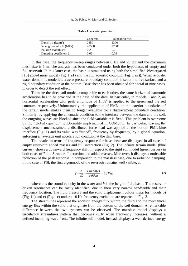
Table 1: material paramters.

Concrete Foundation rock

Density ρ (kg/m3) 2450 2300

Young modulus E (MPa) 20500 22000

Poisson modulus ν 0.2 0.2

Damping coefficient ξ 0.05 0.05

In this case, the frequency sweep ranges between 0 Hz and 25 Hz and the maximum

mesh size is 5 m. The analysis has been conducted under both the hypotheses of empty and

full reservoir. In this latter case, the basin is simulated using both the simplified Westergaard

[16] added mass model (Fig. 1(a1) and the full acoustic coupling (Fig. 1 a2)). When acoustic

water domain is modelled, a zero pressure boundary condition is set at the free surface and a

rigid boundary condition at the bottom. Base shear has been obtained for a total of nine cases,

in order to detect the soil effect.

To make the three soil models comparable to each other, the same horizontal harmonic

acceleration has to be provided at the base of the dam. In particular, in models 1 and 2, an

horizontal acceleration with peak amplitude of 1m/s2 is applied to the green and the red

contours, respectively. Unfortunately, the application of PMLs on the exterior boundaries of

the terrain model makes them no longer available for a displacement boundary condition.

Similarly, by applying the cinematic condition to the interface between the dam and the soil,

the outgoing waves are blocked since the field variable u is fixed. This problem is overcome

by the “global equation” functionality implemented in COMSOL. In particular, leaving the

displacement unconstrained, a distributed force load was applied at the bottom PML blue

interface (Fig. 1) and its value was “tuned”, frequency by frequency, by a global equation,

enforcing an average unit acceleration condition at the dam base.

The results in terms of frequency response for base shear are displayed in all cases of

empty reservoir, added masses and full interaction (Fig. 2). The infinite terrain model (blue

curves), shows a downward frequency shift in respect to the rigid soil model (green curves) in

both cases of Fluid Structure Interaction and added masses. Moreover, it displays a noticeable

reduction of the peak response in comparison to the massless case, due to radiation damping.

In the case of FSI, the first eigenmode of the reservoir remains well visible, at

(2)

where c is the sound velocity in the water and h is the height of the basin. The reservoir

driven resonances can be easily identified, due to their very narrow bandwidth and their

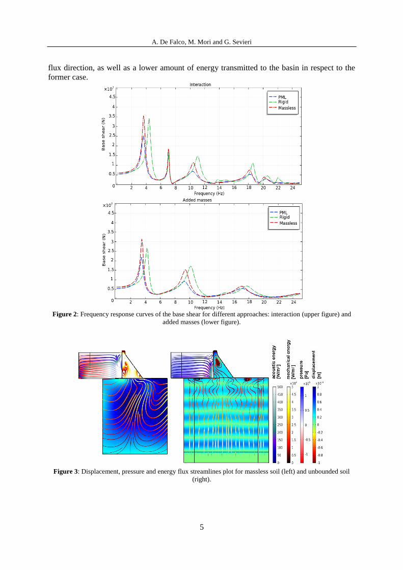
frequency location. The fluid pressure and the solid displacement colour maps for models b)

(Fig. 1b) and c) (Fig. 1c) under a 10 Hz frequency excitation are reported in Fig. 3.

The streamlines represent the acoustic energy flux within the fluid and the mechanical

energy flux within the solid that originate from the bottom of the soil domain. A remarkable

difference between the two systems can be observed. The massless model displays a

circulatory streamlines pattern that becomes curly when frequency increases, without a

defined incoming wave front. The infinite soil model, instead, displays a well-defined energy


5

flux direction, as well as a lower amount of energy transmitted to the basin in respect to the

former case.

Figure 2: Frequency response curves of the base shear for different approaches: interaction (upper figure) and

added masses (lower figure).

Figure 3: Displacement, pressure and energy flux streamlines plot for massless soil (left) and unbounded soil

(right).


6

4 PARAMETRIC ANALYSIS

In order to evaluate the effect of the change in stiffness and density of soil, a parametric

study is performed on a model in the case of empty and full reservoir, allowing a deeper

understanding of the terrain contribution. In Fig. 4 response curves in term of base shear are

shown for empty reservoir and full reservoir, varying the soil stiffness Eg and density g. The

corresponding parameters of concrete are kept unchanged (Table 1). The graphs are expressed

in function of the logarithm of the ratio between the terrain parameter and the corresponding

concrete value in Table 1. Soil parameters are varied one at a time, on a wide range of values,

well beyond a realistic distribution, to emphasize the different effects of each one. It may be

deduced that

For increasing values of the terrain stiffness, both the frequency and the amplitude of the

peak response increase.

For increasing values of the terrain density, the peak response decreases while its

frequency location remains unchanged.

If the terrain has some flexibility, the system’s resonant frequency is always lower than

the rigid case, regardless of terrain density.

In case of full reservoir, the peak of the first frequency of the basin is always evident and

even more noticeable with increasing density and decreasing stiffness.

As expected, the asymptotic response for very stiff terrain converges to the rigid

foundation model (black dashed line). Results obtained from the response analysis in terms of

crest acceleration display the same features as the base shear curves.

Figure 4: Parametric variation of base shear response curve with soil relative stiffness and density – full

reservoir (on the left), empty reservoir (on the right).


7

5 SIMPLIFIED MODEL CALIBRATION

In the previous section the importance of taking into account the unbounded soil in the

dam model has been highlighted. Unfortunately, the aforementioned tools for simulating the

soil behaviour are not always available in each program code or some of them may not be

compatible with time domain analyses. For this reason, in this section a suitable 2D simplified

model is going to be calibrated. It is capable to take into account the SSI using tools and

standard boundary conditions, that are commonly available in all FEM software packages.

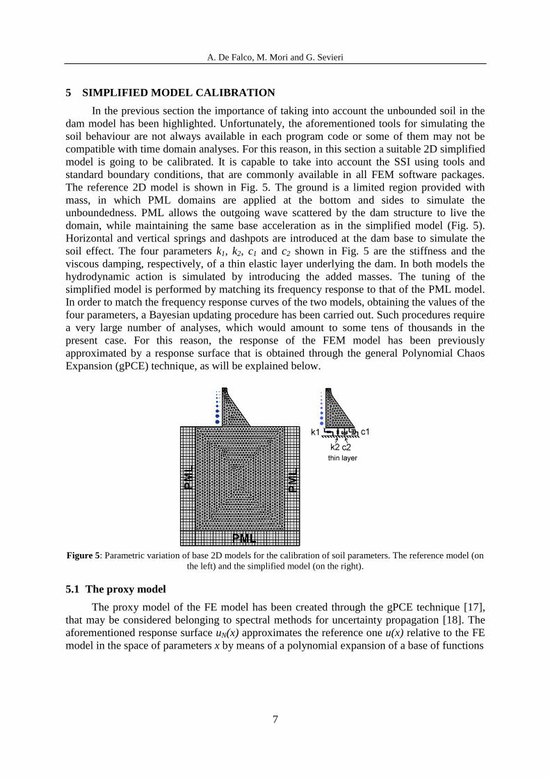
The reference 2D model is shown in Fig. 5. The ground is a limited region provided with

mass, in which PML domains are applied at the bottom and sides to simulate the

unboundedness. PML allows the outgoing wave scattered by the dam structure to live the

domain, while maintaining the same base acceleration as in the simplified model (Fig. 5).

Horizontal and vertical springs and dashpots are introduced at the dam base to simulate the

soil effect. The four parameters k1, k2, c1 and c2 shown in Fig. 5 are the stiffness and the

viscous damping, respectively, of a thin elastic layer underlying the dam. In both models the

hydrodynamic action is simulated by introducing the added masses. The tuning of the

simplified model is performed by matching its frequency response to that of the PML model.

In order to match the frequency response curves of the two models, obtaining the values of the

four parameters, a Bayesian updating procedure has been carried out. Such procedures require

a very large number of analyses, which would amount to some tens of thousands in the

present case. For this reason, the response of the FEM model has been previously

approximated by a response surface that is obtained through the general Polynomial Chaos

Expansion (gPCE) technique, as will be explained below.

Figure 5: Parametric variation of base 2D models for the calibration of soil parameters. The reference model (on

the left) and the simplified model (on the right).

5.1 The proxy model

The proxy model of the FE model has been created through the gPCE technique [17],

that may be considered belonging to spectral methods for uncertainty propagation [18]. The

aforementioned response surface uN(x) approximates the reference one u(x) relative to the FE

model in the space of parameters x by means of a polynomial expansion of a base of functions


8

i(x) = i1(x), ... iN(x) (3)

uN(x) is defined by polynomials up to the N order, whose formulation depends on the

probability density functions type for x [17]

( ) ∑ ̂ ( )

(4)

In the previous equation, ûi is the combination coefficient that is relative to the value of

the multi-index [i] = (i1, i2, iN) [17], [18]. Coefficients ûi are calculated on the basis of the FE

model response. Once the response surface is obtained and the acceptability of the error is

evaluated [19], the statistical properties of the model response can be easily deduced [17]. In

this work, in the absence of prior information on the four parameters, a uniform distribution

was assigned to each one using Legendre polynomials. The number of coefficients ûi to be

determined is obtained from the combinatorial calculation. The number of analyses to be

performed on the FE model is (1+N)p, where p is the number of random variables to be

updated. By choosing polynomials order up to 7, 4096 analyses should be performed for each

set of parameters sampled according to the full-grid rule [17]. Each set can be interpreted as

integration point in the random variables space. In the present case, coefficients ûi have been

determined by a regression of the FE model results [20]. A suitable MATLAB® program [21]

has been written on the base of a functions’ library developed at the Institute of Scientific

Computing of TU Braunschweig. The program automatically recalls COMSOL Multiphysics®

software and processes obtained results.

5.2 Bayesian updating

Once the proxy model has been created, the updating of the mechanical characteristics

of the simplified model has been performed within a probabilistic framework using the

Bayes’s theorem. Let be y = (y1, y2, …, ym) the vector collecting m new observations and x =

(x1, x2, …, xn) the vector of the n unknown parameters. The well-known Bayes’s rule can be

written according to Fisher (1922) [22], introducing the likelihood function L(x, y)

p(x|y) = kL(x,y) p(x) (5)

where p(x) is the probability of the unknown parameters and k is a normalizing factor,

necessary to ensure that the posterior distribution p(x|y) integrates or sums to one. In this

work a q-dimensional multivariate probabilistic model in an additive form has been used [23].

The relation between the h-th measured quantity Ch(x, ) and the related deterministic model

ĉh(x) can be written as follows

Ch(x, ) = ĉh(x) + h h h = 1,…,q (6)

where is the covariance matrix of the random variables h h; h is a normal random

variable with zero mean and unit variance and h represents the standard deviation of the h-th

residual rh(x), which could be seen as the h-th global error


9

rh(x) = Ch - ĉh(x) (7)

Finally, the likelihood function can be linked with the residuals by the following

formula

L(x,) p [⋂ ( h h = h ) )h ]. (8)

In this case, the target to be matched is the frequency response curve of the resultant

base shear. The unknown parameters are the elastic and damping characteristics of the thin

layer k1, k2, c1 and c2. In order to stabilize the variance of the probabilistic model and to

satisfy the homoskedasticity [4], a transformation of the reference quantity, the base shear, is

introduced using a logarithmic function [24]. Thus, Ch is the logarithm of the base shear

Vh (x) obtained for the h-th frequency

Ch (x) = log (Vh (x)) (9)

The frequency response curve is given in steps of 0,1 Hz and the problem may thus be

treated as discrete. In this case, the Markov Chain Monte Carlo (MCMC) resolution method

has been used.

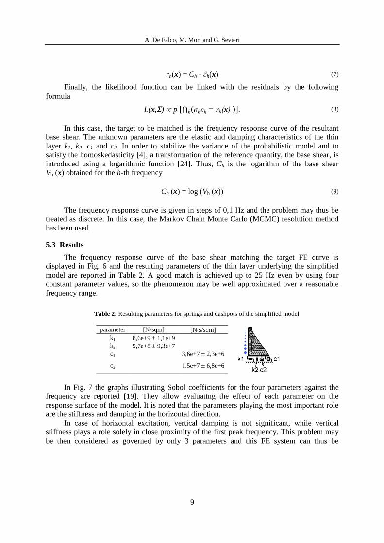
5.3 Results

The frequency response curve of the base shear matching the target FE curve is

displayed in Fig. 6 and the resulting parameters of the thin layer underlying the simplified

model are reported in Table 2. A good match is achieved up to 25 Hz even by using four

constant parameter values, so the phenomenon may be well approximated over a reasonable

frequency range.

Table 2: Resulting parameters for springs and dashpots of the simplified model

parameter [N/sqm] [Ns/sqm]

k1 8,6e+9 1,1e+9

k2 9,7e+8 9,3e+7

c1 3,6e+7 2,3e+6

c2 1.5e+7 6,8e+6

In Fig. 7 the graphs illustrating Sobol coefficients for the four parameters against the

frequency are reported [19]. They allow evaluating the effect of each parameter on the

response surface of the model. It is noted that the parameters playing the most important role

are the stiffness and damping in the horizontal direction.

In case of horizontal excitation, vertical damping is not significant, while vertical

stiffness plays a role solely in close proximity of the first peak frequency. This problem may

be then considered as governed by only 3 parameters and this FE system can thus be


10

simulated with a simplified model with only 2 frequency-independent springs and 1

horizontal dashpot.

Figure 6: Frequency response matching after parameter’s Bayesian Updating.

Figure 7: Sobol coefficients for the four parameters.

6 CONCLUSIONS

The main contribution of this work is to highlight the importance of modelling SSI for

gravity dams and to define a simplified terrain model. At first, different modelling strategies

are compared, in order to investigate the advantages of correct soil effect modelling. A

parametric analysis allowed us to assess the overall SSI behaviour of the system varying soil

properties, density and stiffness. Afterwards, a 2D FE simplified model has been calibrated

through more refined numerical simulations that are available in the literature and are

implemented in the commercial software.


11

This study represents a first step towards assessing the consequences of the variability

of soil characteristics on the calibration of the simplified model proposed in this article.

As future developments, the same analysis will be repeated considering the fluid-

structure interaction, also performing the error updating. The extension of this work to the

three-dimensional case will be carried out.

REFERENCES

[1] Wolf, J.P. Dynamic Soil Structure Interaction. Englewood Cliffs, New Jersey NJ,

Prentice-Hall, (1985).

[2] Clough, R.W. Non-linear mechanisms in the seismic response of arch dams.

Proceedings of the International Conference on Earthquake Engineering, Skopje,

Yugoslavia, June/July, 1980 (1980) 1:669-684.

[3] Tan, H. and Chopra, A.K. Earthquake analysis of arch dams including dam-water

foundation rock interaction. Earthquake Engineering and Structural Dynamics (1995)

24:1453-1474.

[4] Lysmer, J. and Kuhlemeyer, R.L. Finite dynamic model for infinite media. J. Eng.

Mech., ASCE (1969) 95:859-878.

[5] Lofti, V., Tassoulas, J.L. and Roesset, J.M. A technique for the analysis of dams to

earthquakes, Earthquake, Engineering & Structural Dynamics, (1987) 15: 463–490.

[6] Kim, D.K. and Yun, C.B. Time domain soil-structure interaction analysis in two

dimensional medium based on analytical frequency-dependent infinite elements. Int. J.

Numer. Meth. Eng. (2000), 47:1241-1261.

[7] Yun C.B., Kim D.K. and Kim, J.M. Analytical frequency-dependent infinite elements

for soil-structure interaction analysis in two-dimensional medium. Engineering

Structures, (2000), 22:258-271.

[8] Feltrin, G. Absorbing boundaries for the time-domain analysis of dam-reservoir-

foundation systems. Report Swiss Federal Institute of Technology Zurich, (1997).

[9] Yazdchi, M., Khalili, N. and Valliappan, S. Nonlinear seismic behaviour of concrete

gravity dams using coupled finite element-boundary element technique. International

Journal for Numerical Methods in Engineering, (1999), 44:101-130.

[10] Song, C. and Wolf, J.P. The scaled boundary finite-element method, a primer: solution

procedures. Comput. Struct., (2000), 78:211–225.

[11] Givoli, D. High-order local non-reflecting boundary conditions: a review. Wave. Mot.,

(2004), 39:319–326.

[12] Johnson, S. Notes on perfectly matched layers (PMLs). Massachusetts Institute of

Technology, Tech. Rep. (2007).

[13] Berenger, J.P. A perfectly matched layer for the absorption of electromagnetic waves, J.

Comput. Phys., (1994), 114:185-200.

[14] COMSOL® Multiphysics, Use ’s Guide, Version 5.3, COMSOL (2017).

[15] Westergaard, H. M. Water pressures on dams during earthquakes, Trans. ASCE, (1933),

98:418-433.

[16] Kuhlemeyer, R.L. and Lysmer, J. Finite Element Method Accuracy for Wave

Propagation Problems. Journal of the Soil Dynamics Division, (1973), 99:421-427.

[17] Xiu, D. Numerical Methods for Stochastic Computations: a Spectral Method Approach.


12

Princeton University Press, (2010).

[18] Ghanem, R.G. and Spanos, P.D. Stochastic Finite Elements: A Spectral Approach.

SpringerVerlag (1991).

[19] Sudret, B. Uncertainty propagation and sensitivity analysis in mechanical models,

contribution to structural reliability and stochastic spectral methods, Habilitation

Thesis. Université Blaise Pascal - Clermont II (2007).

[20] Matthies, H.G. Uncertainty Quantification with Stochastic Finite Elements Part 1.

Fundamentals. Encyclopedia of Computational Mechanics, John Wiley and Sons, Ltd.

(2007).

[21] The Mathworks Inc. MATLAB - MathWorks.

[22] Fisher, R.A. On the Mathematical Foundations of Theoretical Statistics. Philos Trans R

Soc A Math Phys Eng Sci. (1922) 222:309-368.

[23] Gardoni, P., Der Kiureghian, A. and Mosalam, K.M. Probabilistic Capacity Models and

Fragility Estimates for Reinforced Concrete Columns based on Experimental

Observations. J Eng Mech. (2002) 128:1024-1038.

[24] Yang, Z.A. Modified family of power transformations. Econ. Lett. (2006), 92:14-19.

simplified soil-structure interaction models for concrete gravity...

Documents