PROCEEDIZGS OF THE IEEE VOL. 53: so. 12 DECEMBER. 1965

Simplified Normal Mode Treatment of Long-Period Acoustic-Gravity Waves

in the Atmosphere W. C. MEECHAN

Abstract-This paper deals primarily with the effects of geometric dispersion on low-frequnncy mechanical waves generated by nuclear explosions. This dispersion is the result of the stratitication of the atmosphere (to be distinguished from dispersion due to changes in physical characteristics due to changing frequency). It is found that the pressure signal can be divided naturally into an early-arriving acoustic-gravity portion (treated in this report) and a later-by about five percent of the travel time-acoustic portion.

In general, both portions of the signal are inversely proportional to the range (geometric spreading included), although, at very great ranges, portions of the gravity wave fall off faster by r1/6; the effect of dispersion is to reduce the signal by r-lI2. Most of the signal is composed of many propagating modes which, at a given time and range, will each demonstrate a characteristic frequency. A simplified treatment of this complicated model picture is presented here. It is argued that a ray treatment for the higher-frequency portion is appropriate. It is shown that the frequency of the long-period signal increases with time. So long as the frequency of the received signal is less than the characteristic frequency of the initiating explosive impulse, it is found that the signal pas a universal form for the funda- mental mode. Such characteristics as yield, range, and phase velocity merely change the scaling of the signal. It is concluded that attenua- tion is probably not important for the low-frequency signals (below one c/s) usually observed.

T I. INTRODUCTION

HIS PAPER deals primarily with the effects of geometric dispersion on low-frequency mechanical waves generated by nuclear explosions. We begin

by commenting that geometric dispersion in general reduces the signal amplitude by an amount proportional to + I 2 , where r is the range [l]. That this is so can be seen by the following. Suppose the amplitude of the wave train is A . The time duration of the disturbance, after some time, becomes proportional to the range as a result of dispersion. Total energy must be conserved (neglecting attenuation), so we have approximatel\-

A2r = constant.

Hence A , as suggested. This reduction is in addi- tion to that caused by geometric spreading.

The characteristics of low-frequency, atmospheric, acoustic-gravity waves have been investigated by a number of authors. Such waves can be generated by natural events as well as by nuclear explosions. We shall

this paper was supported and monitored by the Advanced Research Manuscript received August 25, 1965. The research reported in

Projects Agency under Contract SD-79. The author is with the University of Minnesota, Minneapolis,

Minn., and the RAND Corporation, Santa Monica. Calif.

restrict the discussion largely to the latter. S o attempt will be made here to compile a complete bibliography on the subject. However, we should mention normal mode calculations performed by Pfeffer [2], Pfeffer and Zarichny [ 3 ] , Harkrider [4], and Pierce [ 5 ] . Harkrider has succeeded in calculating the expected low-frequency signal (hereafter this term, and the term long-period, mean waves with periods of more than one minute). He used five modes in the rather complex calculations. I t is the major purpose of this report to attempt to obtain the essential characteristics of the low-frequency signal more simply (and, of course, less accurately).

The appropriate mathematical theory for the long- period characteristics of acoustic-gravity waves is given in Pfeffer [2]. From the outset, we distinguish between those waves for which gravitational effects are impor- tant (periods greater than 60 seconds) and acoustic waves (periods less than about 60 seconds). For the former, a normal mode treatment is indicated, as pur- sued in the literature [2]-[5]. M'e examine some of the expected characteristics of such waves in this paper on the basis of simplified models. For intermediate periods (from 30 to 120 seconds), the situation is one where we must still use normal mode methods, but where a num- ber of normal modes can propagate. For the acoustic part of the signal, a very great number of modes can propagate and a ray treatment is more useful.

Lye introduce here a discussion of the normal mode treatment. For our purpose it will be assumed that we observe the mode in the radiation zone, where kr>>l, with k a typical propagation constant. Then we have for the pressure of the nth mode

P,, = G(r)E,(w, Z,)E,(w, Z)eikn(u)riur, (1)

where G ( r ) is a geometric spreading factor with

G(r) = y - l l ? (2)

for propagation in a flat-earth atmosphere (see subse- quent discussion), E , is the excitation function for point excitation,' 20 is the source height, 2 is the receiver height (set equal to zero for ground-level detection), k, =u/cpn, with c,, the phase velocity of the nth mode. I t is assumed in (1) that the excitation is a single-frequency continuous wave. For the usual pulse excitation, we take

1 For details of the excitation process, see Harkrider [4].

2079

2080 PROCEEDISGS OF THE IEEE DECEMBER

the Fourier Transform (F.T.) of the initiating distur- bance to find that

P, = - '(') J ~ ( o ) E , ( w , z ,>E,(w, Z ) e i k n ( w ) r - i a f d w , (3) 2T

where we assume the excitation pressure P(t) has the F.T. P :

~ ( u ) = J eiwtp(t)dt. (4)

The function f ( t ) is found by taking the pressure a t a range far enough from burst so that the overpressure is a small fraction of the ambient pressure, but not so far that the inhomogeneous characteristics of the medium influence the pulse form. Admittedly, i t may be difficult to find such an intermediate range for large yield events. In such a case, we mean by p the linearized pressure disturbance which would be observed in an infinite homogeneous medium. The empirically observed form of the pressure is approximately [6]

N ) = 0 t < O

( 5 )

where t+= Y1I3 t l , f l = 1.0 second, and Y is the yield in KT. The overpressure P o is also proportional to Pia. I t is emphasized that the numerical value of t+ is somenhat uncertain.2 The F.T. of (5) is

- ( - iu) P ( w ) = p o --

( t i ' - i w ) ?

\Ye discuss the calculations which are available for the functions appearing in (3). For simplicity the calcula- tions have been performed assuming a horizontal atmo- sphere. This is adequate for ranges which are less than a quarter of the circumference of the earth. For greater ranges we should take into account the lack of further geometric spreading, due to the spherical earth. It seems reasonable to include, approximately, such effects by modifying the relation (2) for the geometric factor. Thus, for the usual case where wavelengths are small compared with Re, the radius of the earth, we have

(7)

with r measured along the surface of the earth. The focus at the antipode r=nR, is smeared, due to the fact that

* There are two largely unresolved difficulties in the determi- nation of t+. First, it might be that, with a large burst, the first im- pulse takes on a nonspherical form before it becomes linearized, due

a source function more complicated than a simple source function. to atmospheric inhomogeneities. In such a case it is necessary to use

Second, the time of the positive phase t+ is not well known. In Glas- stone [6], p. 117, t+ has not attained its asymptotic value at the max- imum range shown. On the basis of known information, this value must be estimated. (The author is indebted to T. F. Burke of the R A S D Corporation for this statement.)

different earth paths have different winds and thus different propagation mum value at the antipode is

temperatures and times. The maxi-

where a, on the order of a few percent, is the fractional change in group velocity for different paths. Other ef- fects aside, u-e see that the focusing effect might be appreciable. An interesting consequence of (7 ) is that after traveling a ' fraction of the circumference of the earth, the signal shows no further reduction in amplitude due to geometric spreading. Observed reduction in signal amplitude with range must then be due to possible a t - tenuation (usually negligible in situations of greatest practical interest) or dispersion, which is the main effect.

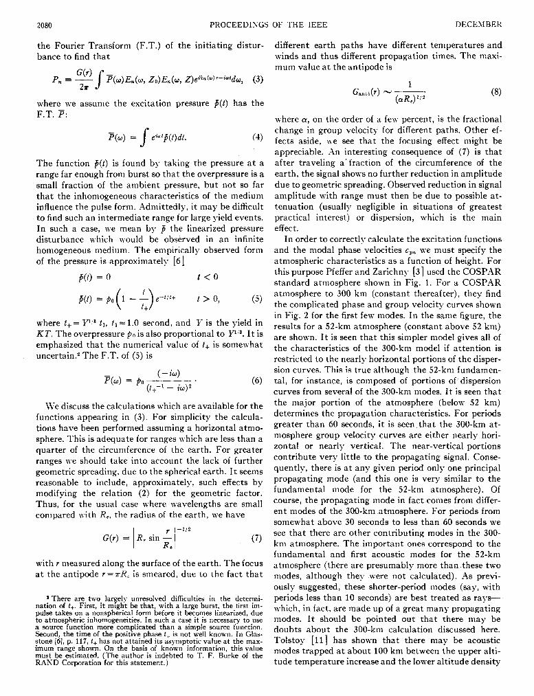
In order to correctly calculate the excitation functions and the modal phase velocities cpn we must specify the atmospheric characteristics as a function of height. For this purpose Pfeffer and Zarichny [3] used the COSPAR standard atmosphere shown in Fig. 1. For a COSPAR atmosphere to 300 km (constant thereafter), they find the complicated phase and group velocity curves shown in Fig. 2 for the first few modes. In the same figure, the results for a 52-km atmosphere (constant above 52 km) are shown. I t is seen that this simpler model gives all of the characteristics of the 300-km model if attention is restricted to the nearly horizontal portions of the disper- sion curves. This is true although the 52-km fundamen- t a l , for instance, is composed of portions of'dispersion curves from several of the 300-km modes. I t is seen that the major portion of the atmosphere (below 52 km) determines the propagation characteristics. For periods greater than 60 seconds, i t is seen that the 300-km at- mosphere group velocity curves are either nearly hori- zontal or nearly vertical. The near-vertical portions contribute very little to the propagating signal. Conse- quently, there is a t any given period only one principal propagating mode (and this one is very similar to the fundamental mode for the 52-km atmosphere). Of course, the propagating mode in fact comes from differ- ent modes of the 300-km atmosphere. For periods from somewhat above 30 seconds to less than 60 seconds we see that there are other contributing modes in the 300- km atmosphere. The important ones correspond to the fundamental and first acoustic modes for the 52-km atmosphere (there are presumably more than .these two modes, although they were not calculated). -4s previ- ously suggested, these shorter-period modes (say, with periods less than 10 seconds) are best treated as rays- which, in fact, are made up of a great many propagating modes. I t should be pointed out that there may be doubts about the 300-km calculation discussed here. Tolstoy [ll ] has shown that there may be acoustic modes trapped at about 100 km between the upper alti- tude temperature increase and the lower altitude density

C ( C O M P R E S S I W WAVE SPEED)

24.9 99.5 224 398 622 895 1219 lW2 2U5 2488 3011 3583 TEMPERATURE *A

200 300 400 500 600 700 800 900 1000 IIOO 1200 m set*

300 km COSPAR

1081

Fig. 1. Average vertical variation of absolute temperature in the atmosphere (estimated by the Committee on Space Research: details up to 120 km given in insert [2]).

Fig. 2. Phase and group velocity curves model atmospheres [2].

for COSPAR

J 0

1 I IO 2 0 3 0 40 5 0 70 :0 ; 200 330 500 I

PERIOD (sec)

------l

PERiOD ( s e d

2082 PROCEEDISGS OF THE IEEE DECEMBER

increase. I t is expected that such an effect will not influ- ence the propagation of periods of interest here because of the attenuation at such altitudes.

I t is interesting to note that the 52-km fundamental mode is made up of acoustic modes from the 300-km calculation for periods of less than 250 seconds and of gravity modes from the 300-km calculation for greater periods.

We shall, in what follows, generally restrict the dis- cussion to the simpler dispersion curves taken from the calculations for the 52-km atmosphere. We see that the long-period gravitational contributions might be ex- pected to arrive with a group velocity about five percent greater (five percent less travel time) than the shorter- period acoustic signals. Of course, this observation ap- plies to the quasi-horizontal portions of the dispersion curves. The reader is referred to [2] , [SI, and [6] for more details concerning the normal mode calculations.

In the next section, we shall simplify the problem by considering the behavior of a given normal mode a t great ranges. I t will be seen that, as previously sketched, due to the dispersion caused by the stratified inhomo- geneity of the atmosphere, the signal amplitude reduces with range. This and other characteristics of the signal will be obtained from (3). The discussion of possible attenuation effects appears in Section IV.

11. SIGNAL DISPERSION For long-period acoustic-gravity waves, we use the

method of stationary phase to approximately evaluate (3). For large r and t , P and E, are slowly varying func- tions of w compared with the exponential. Then, follow- ing standard methods, we look for the stationary point of the argument of the exponential, which is seen to be wn given by

t k; (w,) cgn-l = - . (9) I

Here wn is the nth mode frequency, if there is one, whose group velocity is equal to r / t . Then we have for that stationary contribution, at the frequency w,-given by (9)

P, = G(s)eitn(YR)r-- iYl l tEn(wn, ZO)E,(w,, Z)P(w,)

using

obtained from (9). Equation (10) isvalid in general, when c,’ is not too small [see condition (IS)], and when the range is large, usually

knr >> 1. (1 2 )

The observed signal may be a sum of many modal con- tributions of the type given in (10). If conf+O, as, for instance, when the period greatly exceeds 60 seconds, we must modify the treatment. This is done next.

We note from Fig. 2 that for longer periods the 52-km fundamental phase and group velocities .approach ap- proximately constant value^.^ I t is desirable to calculate the expected behavior for this situation. The first acous- tic mode from the 52-km atmosphere can be treated using (10). We assume for long periods (w<<wo) for the fundamental mode, n = 0

with w o the transition frequency (about 2r / r0 where 7 0 = 60 seconds) and

where cpn is the phase velocity for very long periods and Ac, is of the order of the change in the phase velocity, to be obtained by fitting the phase velocity of the funda- mental 52-km mode in Fig. 2. We see from that figure that A c p / c p , = 0.05.

The restriction on con’ for the validity of (10) can be written conveniently in terms of (14). I t is

with ho, the wavelength corresponding to cpn. For values taken from Fig. 2, the left side of (15) is 0.02 for a range of 8000 km; for most ranges of interest (15) is fulfilled,

From (5) and ( 6 ) , note that for ordinary yields Y, the condition that w<<wo implies that we need the low- frequency limit behavior of P in (3). From (6) we see

P = p o t y - iw), w << i+-’. (16)

Similarly, i t is reasonable to believe (and calculations in Harkrider [4] show) that the characteristic frequencies of Eo are of order WO. Then we also need the long-period behavior of EO, seen to be approximately constant;* this value of Eo is subsequently called ELF. Substituting these low-frequency approximations in (3) we find

d

at P ~ . ~ ~ = ~ ( r ) p o i + 2 ~ ~ ~ ( ~ ) ~ ~ ~ ( ~ ~ ) - r L p (17)

with

3 It might be thought from a casual observation of Fig. 2 that there is a similar situation for short periods. However, when the curves are put on a linear rather than a logarithmic plot, it is found that they actually have finite slope as the period tends to zero.

See Harkrider [4], p. 5309.

1965 IIEECHARl: XIODE TREATRIEST OF LOSG-PERIOD ACOUSTIC-GRAVITY \V.IVES 2083

ILp (the response to a delta function excitation) is found by standard methods to be

ILP =

with

Here J I l 3 and K1!3 are the usual Bessel and modified Bessel functions. I t is easily seen from (18) that 7-l is the order of the value of w for which

that is, where the cubic term in the exponential begins to bring about convergence of the integral. The error made by using the low-frequency approximation for P ( w ) in the region w>t+-’ is negligible if

This condition is satisfied for ranges exceeding 100 km. The result of (17)-(20) shows that the medium is essen- tially a low-pass filter for long-period waves when there is concern only with the most important mode, the fundamental.

111. DISCIXSION OF LONG- AND INTERMEDIATE- PERIOD SIGNAL DISPERSIOK

The reader is reminded that here long periods are those over 60 seconds and intermediate periods are those between about 30 and 120 seconds. Under the assumption that for long periods the fundamental mode has group and phase velocities which are nearly con- stant, the result given in (17)-(20) \\-as obtained. The following characteristics appear from (17)-(20) for the early long-period component-sometimes called the gravity wave:

1) The signal arrival time is approximately fixed by the long-period phase velocity c p x . The precursor a t earlier times increases in amplitude exponen- tially. The signal amplitude then, after this (‘cre- scendo,“ increases like ( A t / ~ ) l / ~ , where At = t - ( r / c p x ) . This increase in amplitude continues until At? 3r3t+-*, when frequencies are such that the approximation (16) fails. For later times the more general result given in (10) could be used (see the following). Since the growth in signal amplitude is due to the increase of P(w) with w , an alternative

procedure can be used. We use the pulse transform (6) and the period as a function of At/? given in (22) to approximately correct for the pulse form. For this purpose, multiply (19) by

[ 1 + ( - y I 1 .

iVe assume in such a treatment that the approxi- mate effect of the pulse spectrum is to multiply the signal a t time At by the value of the spectrum function appropriate to the frequency occurring a t t h a t time.

2) The first important signal arrival, when t = r / c P m , has a long period followed by successively shorter- period arrivals (normal dispersion). From (19) i t is seen that using a n for the approximate zeros of the Bessel functions, when (At/r)3’Z > 1, the period for signal delayed by At is

We see the period decreases like the 3 power of the delay in this normally dispersed part of the signal.

3 ) The range dependence is interesting. The ampli- tude of the early part of the low-frequency signal is seen from (17)-(20) to fall off like the $ power of the range due to dispersion [remembering to take the derivative as in (1 7) 1. For ranges con- siderably less than Re, we use (2) for the function G and find that the long-period wave should de- crease in amplitude like r--(’l6). For greater ranges I > Re the dependence is roughly like r--(*i3). The period of the first arrival, a t a given At, increases like r1I2 according to (22). As the range increases, the amplitude decreases and the period increases due to dispersion. Relatively slow decreases in amplitude with range have been found experi- mentally for signals which circle the globe [7]- [8].

4) From (17), and the scaling laws discussed in Sec- tion I, we see that the amplitude is proportional to yield. The signal waveform is otherwise inde- pendent of yield so long as At< 3 ~ ~ t + - ~ . This should be true for the long-period gravity wave, but care must be used when the delay is such that

2084 PROCEEDINGS OF THE IEEE DECEMBER

the wave merges with the shorter-period com- ponents. For At >3&+-*, so that w<t+-l, we see the signal has a universal form. The yield, range, and atmo- spheric effects enter the scale of the amplitude (for yield) and the time scale (for range and atmo- spheric effects).

These characteristics are also obtainable using the simple stationary phase treatment given by (10). I t is emphasized that the result applies only to the funda- mental mode (as defined for the 52-km atmosphere). Often one can expect one or more of the higher modes to appear also, and their effect must be calculated using

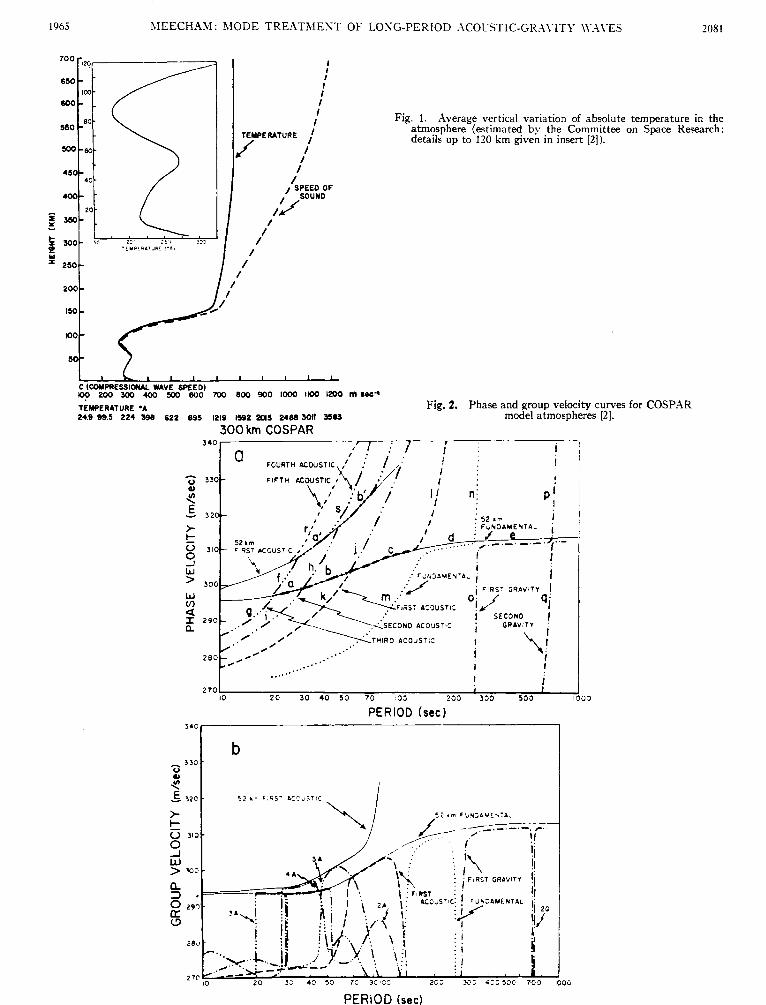
Consider an example: r = lo4 km, w o = 2n/’60, Acp/cpm = 0.05, c,, = +km,/s. Then we find 7 E;: 50 seconds. Ac- cordingly, the result (17)-(20) is valid for A t > 3 ~ ~ f + - ~ ; and with Y = 4 M T , t+ = 16 seconds, we need At<24 minutes. From (22), for A t = loa seconds, the period T is 115 seconds; for At = 4000, T E;: 55 seconds.

The universal result (17)-(20) is shown in Fig. 3.

( 9 H W .

Fig. 3. Low-frequency universal response of the atmosphere for the fundamental mode.

There the quantity r’(d,idt) ILp(At/T) is plotted. The characteristics, discussed previously, can be seen. The dashed envelope curve gives the approximate modifica- tion due to a 4-SIT pulse form, given by the factor of (21a) (parameters for this curve are those of the ex- ample just completed). I t is interesting to note that the initiation of the signal using the velocity c,, is cor- rectly measured from the first positive maximum. The precursor (At<O) is not actually in conflict with the theorems [9] concerning the velocity of propagation of the signal wave front because of the form of the disper- sion curve. We should use (9)-(10) to calculate the curve when At/r is such that W ~ W O ; for the previous example (4 MT), this means for periods of about one

in the dimensionless units of the graph. However, the approximation (13) is not bad for much higher fre- quencies, so that it is not unreasonable to accept the results for greater time delay.

We turn now to a discussion of the intermediate pe- riods between 30 and 120 seconds.) \Ye use (10) and, in general, we must consider many propagating modes in the signal. The number of modes may be quite large when the period is much less than 60 seconds. We see the following characteristics for the intermediate com- ponent:

1) By referring to Harkridet-s i t is found that the fundamental mode for periods greater than 90 seconds has an excitation function which is con- stant at an alt i tude of 18.5 km. More work needs to be done on the excitation functions in order that the frequency dependence may be examined more closely. As already remarked, we assume that for periods greater than 60 seconds the ex- citation functions are constant.

2) Other things being equal, the amplitude of the nth mode is inversely proportional to the square root of the slope of the modal group velocity for the frequency in question. As suggested above, the most important modes are those whose group velocity curves are most nearly horizontal [see

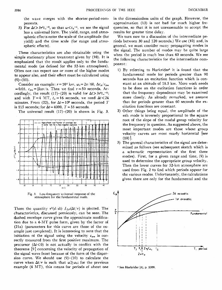
3) The general characteristics of the signal are deter- mined as follows (see subsequent sketch which is a schematic representation of the first three modes). First, for a given range and time, (9) is used to determine the appropriate group velocity. Then the lower curves for 52-km atmosphere are used from Fig. 2 to find which periods appear for the various modes. Unfortunately, the calculations given there are only for the fundamental and the

(10) I .

Fundomental

See Harkrider [A], p. 5309.

1965 1IEECHXhl: AlODE TREAThIENT OF LOSG-PERIOD ACOUSTIC-GRAVITY \V.-\VES 2085

first acoustic modes. The other acoustic modes must be imagined as lying above the first. The slope of the group velocity curve is determined from the calculation. The result is that for an). range and time there can be a great number of modes arriving, each with its appropriate period as explained. We see in the preceding sketch the three periods for the first three acoustic modes a t r , t. Others are not shown. -At a given time many different modes, each with its own frequency, will make up the signal, though the fundamental mode is dominant for low frequencies.

4) The periods of the various modes decrease as the time of observation increases (normal dispersion), as can be seen from the sketch. Xormal dispersion is (usually) observed experimentally [7 ] , [8], [ lo]. The characteristic empirical period 2 7 ~ w o - ~ is shown in the sketch. The period for which the pulse form becomes important, 2at+, is also shown; i t is the period below which the simple form of the fundamental (17)-(20) must be modified because of pulse form.

5 ) The amplitude of the signal falls off like r+I2 due to dispersion. For ranges less than Re, there is an additional factor of r- l i2 for geometric spreading, giving an inverse r amplitude dependence which is apparently spherical. This amplitude reduction with range is (approximately) observed experi- mentally. For instance, if we suppose that the pressure wave from a 1-MT nuclear explosion drops to one-tenth ambient pressure a t a range of about ten km, we find for the overpressure a t 10 000 km from the above

(0.1)106

(104/10) PlO 000 = = lOOd cm-?. (23)

This is the approximate size of observed signals [lo]. I t is interesting to note ‘that, without dis- persion, signals would be 30 times the value given in (23), i.e., much larger than signals are found to be from such events. We note from (10) and (18)-(20) that the long-period fundamental grav- ity wave falls off faster with range (by r 1 ’ 6 ) than the intermediate-period (or short-period) wave.

6) The most prominent frequency in the intermediate signal cannot be determined without knowledge of the excitation functions. For short periods where a ray treatment applies, we may expect the signal to show a frequency maximum a t tha t of the pulse maximum umnx = t+-’. Hence, the “frequency” of the signal would be proportional to Er1/3.

7) From (6) and (10) i t is expected that the ampli- tude of the signal would be proportional to PO, that is, proportional to P 3 . However, the excita- tion function can indirectly, through the param-

eter t+ in 7, influence the dependence of the ampli- tude upon yield. The acoustic signal amplitude can, of course, be influenced by fluctuating atmo- spheric propagation characteristics.

Before closing this section, it is useful to express the intermediate-period mode results in terms of the power spectrum function. We use the definition of the power spectrum for a segment 2T0 of record f ( t )

lr P.S.(u) = - 1-4 T o ( W ) I ? (24)

To

Jvith

1 To -4 ~ ~ ( u ) = - e-lUlf(t)df. ( 2 5 )

The result for the power spectrum of the nth mode is found from (10) and (24) to be

2* L o

We assume that the change in on is slight in the record segment time To. The last factor in (26) gives the peak width when i t is determined by To. The total power spectrum is approximately a sum of terms like (26), one for each mode.

I t is also useful to consider the total energy in the nth mode for r > Re

\\-here K is constant, independent of range, and 0 is the azimuth angle about the source. The result must be independent of the range for a loss-free medium. The total energy is given by a sum over terms like (27) , covering all of the propagating modes; we neglect inter- ference effects which do not affect the energy content. The range independence is, of course, a reflection of the fact that geometric dispersion in the medium does not affect the energy of the propagating wave. This sug- gests using the integral of the square of the observed pressure signal, since this quantity would show no reduction with range due to dispersion. I t would de- crease like l / ~ rather than l/+. The range dependence of the energy would be entirely geometric. For r > Re, the average geometric reduction should be slight. For such ranges, we should find

S p 2 ( f ) d t S constant, independent of Y. (28)

Xoise can be removed by subtracting an integral like (28) for the noise signal. I t should be emphasized that

2086 PROCEEDISGS

(28), representing as it does a fraction of the explosion energy, should be proportional to yield. This dependence should be compared with the fractional power yield dependence of some other characteristics. We see from (28), as remarked previously, that since dispersion causes the signal to spread in time proportional to range, we can expect the pressure to be proportional to r-(l'*) for ranges such that r > Re.

For shorter-period acoustic waves, we can employ the full formalism of ray treatment. This will not be done in this report. However, a few outstanding characteris- tics are worth noting. First, the range dependence due to atmospheric stratification is also r--(1'2) as for normal modes. We might expect interference effects due to multipath phenomena for shorter ranges. The most prominent circular frequency in this part of the signal will occur a t (LC)-', the characteristic frequency of the initiating explosion.

IV. SIGNAL ATTENUATION

We shall consider in this section a few of the more prominent attenuation mechanisms. First, we examine absorption due to molecular vibrational relaxation. Using accepted values we have for the attenuation coef- ficient

a 10-9 w*r

1 + w2r' cm-l, r = 0.002 - 0.05 second. (29)

For w = 2 ~ 1 5 , a 5-second period

a - cm-'. (30)

The signal reduces to a fraction of its value in 106 km due to molecular absorption. For periods above a few seconds, we conclude that such attenuation can be neglected.

Consider now the attenuation which would be caused by scattering from velocity irregularities set up by atmospheric turbulence. Due to the pulsed nature of the initiating signal, we shall for simplicity assume that once a signal is scattered it is lost. I t is true that some of such energy is regained, but for the present purpose of estimation we neglect such contributions. Since we are interested here in long-period disturbances, whose wavelengths are usually greater than the scale of atmo- spheric irregularities, we restrict the discussion to Ray- leigh scattering. We find for the attenuation coefficient

a - @a)'- (AN)*, ka < 1 (3 1) 1 a

1 a

- - (AN)' , ka > 1. (32)

(Equation (32 ) is given for completeness.) ' In (31 ) , a is the turbulence scale length; the correla-

tion length, AN is the turbulent velocity fluctuation relative to the speed of sound, and we have assumed that the turbulent eddies are "close-packed," that is, the

OF THE IEEE DECEMBER

medium is fully irregular. The Rayleigh result goes over to a geometrical optics result of the order given in (32) for higher frequencies. A typical scale length for atmo- spheric turbulence is about one km. Taking the maxi- mum attenuation given in (32 ) for a period less than about 20 seconds, and using AN 2: 0.005, a value tippro- priate to the upper atmosphere, we find

a-l- 40 000 km.

Longer periods would give even less attenuation. We conclude that because of the low contrast of turbulent velocity fluctuations, attenuation due to such scatter- ing is negligible for low-frequency waves.

For higher frequencies, although the scattering from turbulent eddies is slight, there can be appreciable re- flection from laminar wind ducts.

More generally, it can be argued from experimental observations (see, for instance, Donn and Ewing [7] and Jones [8]) that there is no appreciable signal attenua- tion a t present ranges of observation. Any attenuation mechanism would give a certain reduction in signal per unit length. Then, if the signal is reduced byattenua- tion to a fraction by traveling a fraction on the way around the earth, it would be reduced by that fraction to the nth power for a path n times as long. But the first reduction due to attenuation must be negligib!e, since no such drastic reduction is observed in subse- quent passes around the earth.

V. CONCLUSIONS

We have examined the effect of dispersion on acoustic- gravity waves generated by nuclear events a t great ranges. I t is shown by using the normal mode calcula- tion of Pfeffer that i t is natural to divide the signal into three parts: low-frequency gravity modes, intermediate- frequency signals, and acoustic signals. The character- istics of the first two were examined in Sections I1 and 111. I t is found that, in general, dispersion causes a reduction of signal amplitude proportional to the square root of the range, regardless of the portion of the signal considered. This is in addition to the reduction due to simple geometric spreading. The additional range de- pendence is sufficient to give the observed reduction in signal level over that expected from ordinary cylindrical spreading.

We summarize the results. In order to calculate the pressure in different period ranges (alternatively for different time delays), see the following.

A . Fundamental Mode For a period greater than 2n/w0 = 60 seconds and 2at+ (alternatively At less than 3(Acp/cpm2)r and 3(Acp/cpm2) (Y/w&+*): use (17)-(20), where i t is assumed the excitation function is constant in frequency. For a period less than either above (alternatively At greater than corresponding quantities above) : US^ (9)-(10).

1965 IIEECHAII: hIODE TREATMENT OF LOSG-PERIOD ACOCSTIC-GR.1\~ITY \V-IVES 2087

B. Higher Modes For all periods use (9)-(10). I t is appropriate to comment on the expected vari-

ability of pressure records. First, it seems reasonable to assume that the gravity waves wi l l exhibit little vari- ability with changes in tropospheric conditions, since they have very great waveiengths. The same cannot be said of the acoustic \vaves (periods less than about 20 seconds). Their wavelengths are of the order of, or less than, the size of prominent features of the lower atmo- sphere. From Fig. 1 it is seen that there is an acoustic velocity maxin1um at about 50 km. This maximum has a width of about ten km, which corresponds to the wavelength of a 30-second period wave. For such periods and shorter, n-e should expect that changes in wind velocity a t 50 km might seriously affect the modal ex- citation functions and to a lesser extent the dispersion curves, or alternatively the ray propagation character- istics. In this \yay, the large and variable winds a t such altitudes might cause considerable variability in the acoustic and perhaps intermediate-frequency signals. This would be particularly true since relatively small changes in wind speed are seen from Fig. 1 to be suffi- cient to cause the disappearance of the lower duct al- together, as observed from the ground.

Another conclusion which should be emphasized is that the integral of the square of the pressure record, the ‘‘energy” in the wave, may serve as a more sensitive characteristic for detection than the signal itself. This is so since such a measure removes the effect of dis- persion. Thus, the range dependence is just that of the (range periodic) geometric spreading. I t is seen that this energy is proportional to yield.

For future work i t is suggested that power spectral functions (P.S.F.’s) be calculated for the signal records in order to determine the signal characteristics along the lines discussed in this report.

Signal variability forms an interesting topic in itself. I t would be helpful to attempt to correlate this vari- ability with upper atmosphere winds. I t will be interest- ing to examine further P.S.F.’s to see the behavior of

the spectral peaks. In particular, the reduction in fre- quency with increased time of travel should be looked for. Such frequency-travel time results can be used to obtain an experimental determination of the group velocity dispersion curves for the various modes. Finally, i t seems desirable to obtain the characteristics of the modal excitation functions for shorter periods and as a function of altitude. It is noted that these functions may yield important information on burst height [see

The results of the simplified calculations discussed in this report have been compared with the more com- plete results of Harkrider [9]. The frequency dispersion and signal amplitudes correspond well, within 10 to 20 percent in the cases considered.

(1) I .

-ACKNOWLEDGMENT

I t is a pleasure to acknowledge many very helpful discussions with P. Tamarkin and T. F. Burke of The RAND Corporation.

REFERENCES R. Latter,?R. F. Herbst, and K. M. Watson, ‘Effect of nuclear explosion, Ann. Rev. Nuc. Sci., vol. 11, pp. 371-418, 1961. R. L. Pfeffer, ‘‘-4 multi-layer model for study of acoustic-gravity nave propagation in Earth’s atmosphere,” J . Atmos. Sci., 1 7 0 1 .

19, pp. 251-255, May 1%2.

gation from nuclear explosions in Earth’s atmosphere,” Geofisica R. L. Pfeffer and J. Zarichny, “Acoustic-gravity naves propa-

Pura E Applicata-Milano, vol. 55, pp. 175-199, May 1963. D. G. Harkrider, “Surface waves in multi-lavered elastic media and Rayleigh and Love w?ves from buried sources in a multi-

5321. Ami1 1964. layered elastic half-space, J . Geophys. Res., vol. 69, pp. 5295-

A. D. Pierce, “Propagation of acoustic-gravity waves from a small source above the ground in an isothermal atmosphere,” The RAND Corporation, RM-3596, May 1963. S. Glasstone, Ed., The Efects sf Nuclear Weafims. Washington. D. C . : U. S. Government Printing Office, June 1957. W . L. Donn and M. Ewing, “Atmospheric waves from nuclear explosions,” J . Atmos. Sci., vol. 19, pp. 264-273, October 1962. R. \’. Jones, “Sub-acoustic waves from large explosions,” Nature, vol. 193, pp. 229-232, January 1962. J. -1. Stratton, Electromagnetic Theory, Sew York: McGraw- Hill, 1941, p. 333 ff. J. S. Hunt, R. Palmer, and Sir LV. Penney, “Atmospheric naves caused by large explosions,” Phil. Trans. Roy. SOC. (London), vol. A252, pp. t75-315, February 1960. Ivan Tolstoy, The theory of wavesjn stratified fluids including the effects of gravity and rotation, Ref. Mod. Phys., vol. 35, pp. 207-230, January 1963.

I