simplified conceptual structures and analytical …cdn.intechopen.com/pdfs/32916.pdf · simplified...

10

Simplified Conceptual Structures and Analytical Solutions for Groundwater Discharge

Using Reservoir Equations

Alon Rimmer1 and Andreas Hartmann2 1Israel Oceanographic and Limnological Research Ltd.,

The Yigal Alon Kinneret Limnological Laboratory, 2Institute of Hydrology, Freiburg University,

1Israel 2Germany

1. Introduction

The approaches to the study of hydrological issues are generally divided into two very different groups: (1) the physical approach; and (2) the system approach (Singh 1988). The physical approach is motivated primarily by scientific study and understanding of the physical phenomena, whereas the practical application of this knowledge to engineering and water resources management is recognized but not always fully required. Unlike detailed physical studies of each hydrological problem, the system approach is driven by the need to establish working relationships between measured parameters for solving practical hydrological problems. This approach simplifies the issue because it is unfeasible to consider the entire physical system. Therefore, a logical approach consists of measuring those variables in the hydrologic cycle, which appear significant to the problem, and establish explicit mathematical relationships between them.

An initial step and a well-recognized part of groundwater flow analysis is the definition of a conceptual model. It is usually a simplified perception of the dominant physical components of the studied groundwater system. The main purpose for constructing a conceptual model is concentrating on the parts relevant for solving the hydrological problem.

Common ways to convert a conceptual model of a groundwater system into mathematical formulations are reservoir (or ‘tank’) type models (Dooge, 1973; Sugawara, 1995). These model types are often used as a theoretical tool in surface and subsurface hydrology, for water management, control of inflows and outflows in lakes, rivers, reservoirs, and aquifers. The linear reservoir concept is an important component of many widely used hydrological models like the TOPMODEL (Beven & Kirby, 1979), HBV (Lindström et al., 1997) or WaSiM-ETH (Schulla & Jasper, 2007). Reservoir type models are especially useful in karst environments, because the essential information for physical approaches is usually not available (Jukic & Denic-Jukic, 2009). The lack of information and the necessity to use simplified reservoir models become evident in the high number of recently published studies on karst hydrology (Fleury et al., 2007; Geyer et al., 2008; Hartmann et al., 2011; Jukic & Denic-Jukic, 2009; Kessler & Kafri, 2007; Le Moine et al., 2008; Rimmer & Salingar, 2006; Tritz et al., 2011).

www.intechopen.com

Water Resources Management and Modeling

218

In this chapter, a set of typical groundwater modeling problems is described, exemplifying the use of simple reservoir structures to model spring discharge and/or groundwater level during time. In each example, we will explicate the use of the proposed reservoir type system. Moreover, in each case, we will examine an analytical solution associated with the proposed system using simple domain geometries. The advantage of analytical solutions is that their equations offer quick answers to the proposed mechanism based on a few basic parameters. These solutions therefore allow an immediate system understanding and provide a meaning value for each parameter or group of parameters. Given the differential equation that describes the groundwater system, most of the presented analytical solutions can be found using the ‘symbolic mathematical toolbox’ of MATLAB (http://www.mathworks.com).

2. Examples

Our set of example models include: (1) the classic formation of the linear reservoir problem for an aquifer drained by a single spring; (2) spring discharge potentially fed by two parallel aquifers; (3) spring discharge potentially fed by two serial groundwater aquifers; (4) two parallel aquifers with linear exchange and linear discharges; (5) the discharge from an aquifer with two outlets; (6) the discharge from an aquifer into a lake (submerged springs); and (7) the cases of long-term change of groundwater level and annual spring discharge. Although in most cases the models will be applied with a given set of measured data, it is important to clarify that these types of models are not location-specific, and can be used to model various groundwater flow systems.

2.1 The formation of linear reservoir problem for a single spring discharge

In a traditional hydrology, a spring discharge is often conceptually described and modelled using simple linear reservoirs. We can start the simplification of a system by examining the spring discharge Q (L3 T-1) according to Darcy’s Law:

0( )( ) i

h t HQ t k G

x

(1)

where h (with units of length, L) represents an equivalent unknown hydraulic head in the aquifer, H0 (L) is the head at the spring outlet (if an exact head can be evaluated) so that h-H0 represents the equivalent hydraulic head difference between two points, located at x (L) distance one from the other. The ki (units of length over time, L T-1) is the saturated hydraulic conductivity, and G (L2) represents an “equivalent” cross section of the flow. For practical purposes, it is assumed that ki, G and x are constant for a given natural aquifer, and therefore Eq. 1 can be simplified to:

0 ; ik GQ t h t H

x (2)

considering H0=0 in Eq. 2, further simplification can be conducted by conceptualising the drained aquifer as a reservoir (0) with storage V (L3) varying in time; constant recharge area A (L2) and a given effective porosity n (-):

www.intechopen.com

Simplified Conceptual Structures and Analytical Solutions for Groundwater Discharge Using Reservoir Equations

219

V t A n h t (3)

according to Eqs. 2 and 3, in such a reservoir model, spring discharge through the outlet, Qout, is proportional to storage.

;out

A nV t KQ t K

(4)

where K (given in units of time, T) is known as the reservoir constant or storage, representing the recharge area, the porosity, the saturated hydraulic conductivity, and the equivalent path and cross section of the flow within the aquifer. Usually, changes of K in time or from one season to another are not physically justified, and it should be independent of both the selected period of modeling, and the boundary conditions (amount of precipitation).

The equation for the continuous water balance in this kind of reservoir is:

in out

dV tQ t Q t

dt with 00outQ t Q . (5)

Fig. 1. (a) Schematic description of groundwater system; (b) linear reservoir model

Incorporating Eq. 4 into Eq. 5 results in the linear reservoir differential equation:

0; 0out

in out

dQ tK Q t Q t t t

dt (6)

A well-known application in hydrology is the determination of K. This task becomes significantly easier in the dry period that follows the rainy season, since the flow is then a smooth, physical and unidirectional process, with no random processes (such as rainstorms) to be taken into account. At this time Qin(t)=0 and the mathematical description of linear reservoir model (Eq. 6) reduces to the homogeneous equation:

00 ; 0out out

out

dQ t Q tQ t Q

dt K (7)

Eq. 7 is solved analytically by:

www.intechopen.com


220

0

0

. exp

. exp

out

out

ta Q t Q

K

tb V t KQ t KQ

K

(8)

In Eq. 8, V is the volume (assume 103 m3), t is the time (day), Qout is the outflow (103 m3 day-1), Q0 is the outflow (103 m3 day-1) at the day when Qin vanished, and K is the reservoir constant with units identical to the units of t (day).

Analyzing spring recession in this way is known as Maillet’s approach (Maillet, 1905). An application of this fundamental method is presented in Fig. 2, with measured discharge flow from the Carcara Springs in the Western Galilee, Israel, during the dry period starting in March 1981. The springs emerge from the aquifer of the Upper Judea Group formation, which appears to be connected to the aquifer of the Lower Judea Group formations. In this time of the year, the regional groundwater level is usually high. Data from 1950-1985 indicated that the spring had never dried, a situation that changed significantly since the beginning of pumping in 1985 (These changes are discussed in section 2.5).

0

2

4

6

8

10

12

14

0 60 120 180 240days

Qou

t(1

000

m3 d

ay-1

)

Model

Measured

K=117 days

0

2

4

6

8

10

12

14

0 60 120 180 240days

Qou

t(1

000

m3 d

ay-1

)

Model

Measured

K=117 days

Fig. 2. The discharge of Carcara Spring during the dry period starting in March1981. K was calibrated to 117 days.

2.2 Parallel linear reservoirs

During a dry season that follows a rainy season, the discharge of a spring reduces in time. The shape of the graph discharge vs. time corresponds to the sum of several exponential functions (Bonacci, 1993; Grasso & Jeannin, 1994). Often, such spring discharge is represented as a combination of two parallel linear reservoirs (Fig. 3), mathematically represented by:

1 2

01 021 2

1 1 2 2

.

exp exp

.

out out out

out out

a Q t Q t Q t

t tQ Q

K K

b V t K Q t K Q t

(9)

A simple optimization algorithm can be applied to identify the K1 and K2 constants, as well as the initial flows Q01 and Q02 during a recession period. When K is small, the recession of

www.intechopen.com


221

the reservoir will be fast, and its discharge and volume will reach zero within a short time. When K is large, the recession will be slow, and the reservoir outflow will last for a long time. If K1 >> K2 the discharge from reservoir 2 (second component in the right hand side of Eq. 9) decreases much faster than the discharge from reservoir 1 (first component in the right hand side of Eq.9), which will still be active much longer.

Qout1

h

H0

H1 A1

Qin1

h

H0

H2

K2

A2

Qin2

Qout2

Qout

K1

Fig. 3. Two parallel reservoirs. The reservoirs are fed by groundwater recharge originating from the surface and drain simultaneously to the stream.

The parallel groundwater reservoir structure is incorporated in many hydrological models, e.g., the Vensim model (Fleury et al., 2007). Here it is exemplified by applying it to the recession discharge of the Hermon Stream (Israel) during the year of 1996 (Fig. 4). The stream is one of the three main tributaries of the Upper Jordan River (Rimmer and Salingar, 2006). It is fed mainly by the Banias Spring, located at the edge of the karst exposures on the lower parts of the Hermon Mountain, at an altitude of 359 m a.s.l. The Banias annual average discharge is ~67 M m³ (~2.15 m³/s). The spring exhibits behaviour of pluvio-nival regime, where discharge is mainly due to precipitation, but also slightly influenced by snowmelt (Gilad & Bonne, 1990; Samuels et al., 2010).

0

100

200

300

400

500

600

3/30 5/29 7/28 9/26 11/25 1/24

days

Qou

t(1

000

m3 d

ay-1

)

Reservoir 1Reservoir 2TotalMeasured

Q0 145420

K 30056

Parameter 1 2

0

100

200

300

400

500

600

3/30 5/29 7/28 9/26 11/25 1/24

days

Qou

t(1

000

m3 d

ay-1

)



Q0 145420

K 30056

Parameter 1 2

Q0 145420

K 30056

Parameter 1 2

Fig. 4. Stream discharge of the Hermon stream during 1996. The stream is fed by two parallel reservoirs during the recession period: Since K2>>K1 the reservoir 1 discharge represents most of the sharp changes following the rainy season, while reservoir 2 represents the more stable component.

www.intechopen.com


222

The optimization algorithm revealed that K1 = 56 days and Q01 = 420,000 m3day-1, representing the immediate aquifer that contributes to the spring, while K2 = 300 days and Q01 = 145,000 m3day-1, representing the discharge from a large stable aquifer, which also drains into the Dan Spring located nearby. During the recession period, the discharge of reservoir 1 ceases after ~170 days, while the memory of reservoir 2 remains for ~2.5 years (Rimmer & Salingar, 2006).

2.3 Two serial linear reservoirs

Usually, the discharge recession of a karst spring is fast at the beginning of a dry season and slows at its end (see Eqs. 8 and/or 9). However, there are cases in which the recession is rather slow at the beginning, and increases towards the end of the dry season (Rimmer & Salingar, 2006). Moreover, the recession is faster following a low precipitation season, than after a high precipitation one. One reason for such behaviour can be explained by the interplay of two systems in series, e.g., a large vadose zone on top of the phreatic zone or two groundwater systems of which one is recharged by leakage from the other (Fig. 5a). The pattern analysis of such measured spring discharge requires a different setup. The proposed mechanism for examining this type of observed curve is a system with two serial linear reservoirs (Fig. 5b).

Fig. 5. (a) schematic description of the proposed groundwater system; (b) the system represented by two serial reservoirs. Excess saturation flow from the earth surface feed the upper reservoir (1), which recharges the lower reservoir (2).

In this example, the simplified system is described by an upper linear reservoir, contributing to a lower reservoir, draining through a spring outlet. Similarly to the previous case, we are particularly interested in determining the system storage coefficients K1 and K2, and the initial conditions (flow at the beginning of the dry season) Q01 and Q02. By defining the input to the upper reservoir (1) during the dry season as zero, the input to the lower reservoir (2) is an exponential recession with time, typical to a linear reservoir system (Section 2.1; see also Nash 1957; Huggins & Burney, 1982). We therefore write the differential equation for the lower reservoir (2) for a single dry season as follows:

2 2 1

2 2

1 01 2 02

; 0

1. 0 2. 0 ;

out out out

out out

dQ t Q t Q tt

dt K K

with Q t Q Q t Q

(10)

www.intechopen.com


223

where Q01 and Q02 are the initial conditions, yet to be determined from the measured data of each season. In Eq. 10 the contribution from the upper to the lower groundwater reservoir and the upper reservoir volume are determined by:

1 01

1

1 1 1

expout

out

tQ t Q

K

V t K Q

(11)

and Eq. 10 can be solved analytically so that the discharge from the lower groundwater reservoir and its volume are determined by:

2 2/1 2/2

01 12/1

1 2 1 2

2/2 022

2 2 2

exp exp

exp

out out out

out

out

out

Q t Q Q

Q K t tQ

K K K K

tQ Q

K

V t K Q

(12)

Here, the outflow from the lower reservoir is combined of the contribution from the upper reservoir Qout2/1 and the self-discharge of the lower reservoir Qout2/2. With an optimization algorithm, Eq. 12 may be used to evaluate K1, K2, Q01 and Q02 for each season, so that it

Fig. 6. Illustration of the terms in Eq. 12- the upper reservoir contribution Qout2/1 and the self-discharge of the lower reservoir Qout2/2 combine the total outflow Qout2. The K1 = 70 days and K2 =300 days are identical for both rainy (1993) and dry (1990) years, while the two initial conditions Q01 and Q02 are different. (a, b): 1993; (c, d): 1990. (a, c): spring discharge; (b, d): Aquifer volume.

www.intechopen.com


224

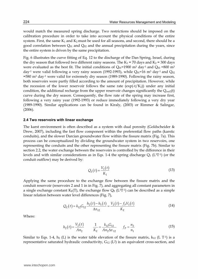
would match the measured spring discharge. Two restrictions should be imposed on the calibration procedure in order to take into account the physical conditions of the entire system. First, the same K1 and K2 must be used for all seasons, and second, there should be a good correlation between Q01 and Q02 and the annual precipitation during the years, since the entire system is driven by the same precipitation.

Fig. 6 illustrates the curve fitting of Eq. 12 to the discharge of the Dan Spring, Israel, during the dry season that followed two different rainy seasons. The K1 = 70 days and K2 = 300 days were evaluated as the best fit. The initial conditions of Q01=1900 m3 day-1 and Q02 =800 m3 day-1 were valid following a very rainy season (1992-1993), while Q01=16 m3 day-1 and Q02

=580 m3 day-1 were valid for extremely dry season (1989-1990). Following the rainy season, both reservoirs were partly filled according to the amount of precipitation. However, while the recession of the lower reservoir follows the same rate (exp(-t/K2)) under any initial condition, the additional recharge from the upper reservoir changes significantly the Qout2(t) curve during the dry season. Consequently, the flow rate of the spring may increase first, following a very rainy year (1992-1993) or reduce immediately following a very dry year (1989-1990). Similar applications can be found in Kiraly, (2003) or Rimmer & Salingar, (2006).

2.4 Two reservoirs with linear exchange

The karst environment is often described as a system with dual porosity (Goldscheider & Drew, 2007), including the fast flow component within the preferential flow paths (karstic conduits), and the slower Darcian groundwater flow within the fissure matrix (Fig. 7a). This process can be conceptualized by dividing the groundwater system in two reservoirs, one representing the conduits and the other representing the fissure matrix (Fig. 7b). Similar to section 2.2, the water exchange between the reservoirs is controlled by the difference in their levels and with similar considerations as in Eqs. 1-4 the spring discharge Q1 (L³T-1) (or the conduit outflow) may be derived by:

11

1

V tQ t

K (13)

Applying the same procedure to the exchange flow between the fissure matrix and the conduit reservoir (reservoirs 2 and 1 in in Fig. 7), and aggregating all constant parameters in a single exchange constant KE(T), the exchange flow QE (L3T-1) can be described as a simple linear relation between water level differences (Fig. 7),

2 1 2 112 12

12

PE

E

h t h t V t f V tQ t k G

x K

(14)

Where:

2 12 12 22

2 2 12 1

1P

E

V t k G nh t f

An K An x n (15)

Similar to Eqs. 1-4, h2 (L) is the water table elevation of the fissure matrix, k12 (L T-1) is a representative saturated hydraulic conductivity, G12 (L2) is an equivalent cross-section, and

www.intechopen.com


225

x12 (L) an average flow distance; all are parameters representing the interface between conduits and fissure matrix.

QIN2 QIN1(b)

QE

KE, fP

A2

Q1

A1

K1

V1

V2

(a)

Qout

h2h1

A

impermeable Fig. 7. (a) Schematic description of the groundwater system with karstic conduits and fissure matrix; (b) the system represented by a reservoir combination with a fissure matrix reservoir (left, 2) and conduit reservoir (right, 1).

With the effective porosity of the fissure matrix n2, and the area A2, the relation between water level and stored water volume V2 (L3) can be established. Note that in Eqs. 13-15 the same area A is used because the simplification approach assumes that the conduits section is embedded within the fissure matrix (double porosity approach) and that the porosity differences between the conduits and fissure matrix were taken into account by the porosity factor fP. With it A, A1 and A2 in Fig. 7 are related to each other as follows:

1 2 1 1 PA A A A f (16)

Having defined the flow processes of the conduit and the fissure matrix, water balance for both reservoirs can be established:

1 2 1 11

1

2 2 12

PIN

E

PIN

E

dV t V t f V t V tQ

dt K K

dV t V t f V tQ

dt K

(17)

Rearranging Eq. (17) results in a linear system of inhomogeneous differential equations:

1 11

2 2

1 1

1

PIN

E E

PIN

E E

fD V t Q

K K K

fD V t Q

K K

(18)

Hereby, D is the differential operator d/dt. Assuming constant inflows QIN1 and QIN2, Eq. (18) can be solved analytically with standard methods (Kramer's rule, variation of constants; e.g. Boyce and DiPrima, 2000) and yield:

1 1 1 2 2 1

2 3 1 4 2 2

exp exp

( ) exp exp

V t B A t B A t C

V t B A t B A t C

(19)

www.intechopen.com


226

With the constants

2

1,21 1 1

1 11 1 1 1 12 4

P P

E E E

f fA

K K K K K K

(20)

10 2 10 2 11 2 10 1 1

1 2

20 2 20 2 23 4 20 3 2

1 2

V A V A CB B V B C

A A

V A V A CB B V B C

A A

(21)

1 1 1 2

2 2 1 1 2

IN IN

E IN P IN IN

C K Q Q

C K Q K f Q Q

(22)

Where V10 and V20 are the reservoir volumes and 10V and 20V the storage change at t= 0.

10V and 20V can be obtained by Eq. 18):

1 20 10 1010 1

1

2 20 1020 2

0

0

PIN

E

PIN

E

dV t V f V VV Q

dt K K

dV t V f VV Q

dt K

(23)

Except for A1,2, the constants, as well as the initial conditions refer to a single time step, and have to be calculated each time step again. For instance at time step t V10 would be equal to V1(t-1) and V20 equal to V2(t-2), respectively.

Methods that consider the exchange between fissure matrix and conduits can be found in Cornaton & Perrochet (2002) and Sauter (1992). In Fig. 8, the exchange reservoirs solution was applied to the last recharge event and the dry season recession in 1998 at the Banias Spring (see section 2.2). The exchange between the conduit and the fissure matrix reservoir resulted in a buffering of the recharge signal and a slow increase in fissure matrix storage. Exchange flow was negative, indicating flow towards the fissure matrix. Around the end of

Fig. 8. Left: stored water in the conduit reservoir V1, the fissure matrix reservoir V2 and total storage V1+V2; Middle: total recharge QIN, spring discharge Q1 and exchange flow QE vs. observed spring flow; Right: conduit and matrix water SO4 concentrations, CConduits and CMatrix, discharge concentrations C1 vs. observed SO4 concentrations

www.intechopen.com


227

April, it changed its direction, which means that parts of the stored water in the fissure matrix were released again to the springs. This switch of direction of the exchange flow was nearly insignificant in terms of flow rates but had immense impact on the water quality. This is exemplified by the SO4 variations observed at the same spring during the same time: by simply attributing constant SO4 concentrations to the conduit and matrix flows their mixing at the spring outlet resulted in an acceptable agreement with the observations.

2.5 The linear reservoir with two outlets

In this section, the case of the effect of additional outlet is discussed. Consider the case of a spring discharge, which differs from the basic case (section 2.1) in two important elements: (1) the spring may dry out completely, so that the exponential recession (Eq. 8) is not valid for low flow rates; and (2) From the water mass balance calculations, it is assumed that the groundwater recharge is larger than the spring discharge, and therefore part of the water continues to flow downstream the aquifer to deeper layers. When these two conditions are valid, the linear reservoir with upper and lower outlets (Fig. 9) may represent the system rather well.

With similar considerations, we can handle the problem in Eq. 5 with two outlets, and no recharge, described as follows:

0 1 1

0 1

; 0

;out out

out

Q Q t tdV t

Q t tdt

(24)

where t1 is the time in which the upper outlet (Qout1) is drying, leaving only the flow in the lower outlet (Qout0).

Qout0

h

Qout1H1

H0

h0 A

Qin

K2, n2

K1, n1

(b)A

Qout1H1

h0

(a)

Qout0

K2, n2

K1, n1

H0

Qin

impermeable

h

Qout0

h

Qout1H1

H0

h0 A

Qin

K2, n2

K1, n1

(b)

Qout0

h

Qout1H1

H0

h0 A

Qin

K2, n2

K1, n1

(b)A

Qout1H1

h0

(a)

Qout0

K2, n2

K1, n1

H0

Qin

impermeable

h

A

Qout1H1

h0

(a)

Qout0

K2, n2

K1, n1

H0

Qin

impermeable

h

Fig. 9. Linear reservoir with two outlets at different levels

If it is assumed that outlet (1) changes the pressure field only locally, we can consider each outflow separately as a linear function of the head above it, so that:

1 1 1

0 2 0

out

out

Q t h t H

Q t h t H

(25)

www.intechopen.com


228

With Eq. 25 incorporated into Eq. 24, assuming no inflow and H0=0 the problem is defined as follows:

1 11 2 1

0

12

1 1 1; 0

; 01

;

h t H t tdh t K K K

with h t hdt

h t t tK

(26)

The analytical solution to the problem in Eq. 26 is:

0 1

1

1 1 2

1 12

exp ; 0

1 1;

1exp ;

C Ch t h qt t t

q q

where

HC q

K K K

and

h t C t t t tK

(27)

In order to keep continuous recession curve, the head at time t1 should be equal to H1, and identical for the two problems, therefore:

1 0 1 1expC C

h t h qt Hq q

(28)

From Eq. 28 we can define the time t1 in which the flow from the upper outlet vanishes. It is a function of 0 1 1 2, ,h H K and K .

1

11

0

lnh H

H C qt t q

h C q (29)

That type of groundwater reservoir is also included in the HBV model (Lindström et al., 1997). An application of the proposed mechanism is presented in Fig. 10, with measured discharge flow from the Carcara Springs in the Western Galilee, Israel, during the dry period starting in March 2002. Note that this spring is similar to the one presented in section 2.1 and therefore K1 was calibrated to 117 days. However, there is a major difference between section 2.1 and 2.5; since the beginning of pumping in 1985, water levels have been dropping significantly, so that the spring has been drying completely almost every dry season since 1995. The drying requires analysing the spring discharge with Eq. 26 rather than with Eq. 7, and additional calibration of K2=100 days, which, as expected, turned to be nearly similar to K1. On the regular scale (Fig. 10a) the difference between a drying and not drying spring is not easily perceived, but it becomes clear, and the value of t1 = 161 days is obvious when plotted on a logarithmic scale (Fig. 10b).

www.intechopen.com


229

0.01

0.10

1.00

10.00

100.00

0 60 120 180 240 300 360days

0

10

20

30

40

50

60

0 60 120 180 240 300 360days

Qou

t1(m

3 sec

-1) Qout1

Qout1,exp

Measured

Log

[Qou

t1(m

3 sec

-1)]

(a) (b)

Fig. 10. The outflows through the upper outlet in a linear reservoir with two outlets in different level Qout1 and, for comparison, the outflow from a regular linear reservoir without lower outlet Qout1,exp . (a) regular scale; (b) logarithmic scale.

2.6 Aquifer drainage to submerged springs

The same physical factors were considered in modelling the process of groundwater discharge into springs onshore and offshore a lake, or a river (Fig. 11). Unlike in previous cases, here, the analytical solution was applied to the entire annual cycle, in order to exemplify the case where the spring outflows are dictated by the downstream head at the lake or river.

h

Qout1

Qout0

z1

h

HL

K1, n1

K0, n0

Qin

(b)(a)

On shore spring

Qin lake

Confined aquifer

impermeable

Observation well

Fig. 11. (a) Schematic description of groundwater system that discharges simultaneously from confined aquifer into springs onshore and offshore a lake. (b) A model where the reservoir drains through a constant level (z1) onshore spring Qout1(t), and a time varying boundary HL(t) representing offshore spring Qout0(t). The hydraulic head within a short distance (up to several hundred meters) from the lake is h(t).

The proposed simplified model aims to link the time-dependent spring discharge to the hydraulic heads in the contributing aquifer under the fluctuations of the lake level. These fluctuations are independent of the aquifer system, and affect the spring flow as a close boundary condition. Here we assume constant recharge Qin, and time dependent discharge from the aquifer to the onshore Qout1(t) and offshore Qout0(t) springs:

1 1 1

0 0

out

out L

Q t h t z

Q t h t H t

(30)

www.intechopen.com


230

We regard the elevation of the onshore spring z1=0, and lake HL level fluctuating as a sin function around an average level. Under these conditions:

1 1

0 0 0 1 1sin

out

out

Q t h t

Q t h t b b t

(31)

Here b0 (m) is the average lake level below the spring outlet (b0 is negative); b1 (m) is the lake fluctuations amplitude; is the angular frequency in radians which for yearly rotations has a set value of 1 2 365.25 ; and is the phase shift (radians). With similar considerations as in earlier problems, we can handle the reservoir mass balance with two outlets, and constant recharge:

0 1in out out

dV tQ Q Q

dt (32)

Incorporating Eq. 31 into Eq. 32 and rearranging using Eqs. 2, 3 and 4 results in:

0 11

1 0 0 0

0

1 1sin

: 0

indh t Q b bh t t

dt K K A n K K

with h t H

(33)

This equation is solved analytically by:

1 100 1 2 2

0 0 1

0 1

cos sinexp( )

1 1

in t q tb Qh t H qt b

K q A n q K q

qK K

(34)

An initial test of this solution reveals that if t , the lake level assumed to be steady with no fluctuations (b1=0), and the inflow Qin=0, then:

0 0

0 0

1

1

b bh t

K q K

K

(35)

From Eq. 35 it can be concluded that if the connection between the aquifer and the lake is significantly stronger than the connection to the onshore spring (K0<<K1), then the aquifer hydraulic head assumes the level of the lake 0h t b , but if K0>>K1 the aquifer hydraulic head adapts to the level of the spring outlet 0h t . If Qin>0 then h(t) increases by Qin resulting higher discharge through the spring outlets. Discharge of an onshore spring Qout1(t) is straight forward to measure. Therefore, we can evaluate it according to Eq. 31 and calibrate 1. However the offshore spring discharge Qout2(t) is usually difficult to measure resulting in infinite possibilities to evaluate it since 0 is also unknown.

www.intechopen.com


231

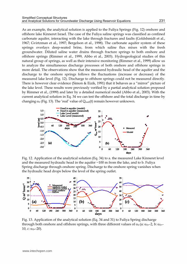
As an example, the analytical solution is applied to the Fuliya Springs (Fig. 12) onshore and offshore lake Kinneret Israel. The case of the Fuliya saline springs was classified as confined carbonate aquifer, interacting with the lake through fractures and faults (Goldshmidt et al., 1967; Gvirtzman et al., 1997; Bergelson et al., 1998). The carbonate aquifer system of these springs overlays deep-seated brine, from which saline flux mixes with the fresh groundwater. Diluted saline water drains through fracture springs to both onshore and offshore springs (Rimmer et al., 1999, Abbo et al., 2003). Hydrogeological studies of this natural group of springs, as well as their intensive monitoring (Rimmer et al., 1999) allow us to analyze the simultaneous discharge processes of both onshore and offshore springs in more detail. The observations show that the measured hydraulic head of the aquifer and the discharge to the onshore springs follows the fluctuations (increase or decrease) of the measured lake level (Fig. 12). Discharge to offshore springs could not be measured directly. There is however clear evidence (Simon & Eizik, 1991) that it behaves as a “mirror” picture of the lake level. These results were previously verified by a partial analytical solution proposed by Rimmer et al., (1999) and later by a detailed numerical model (Abbo et al., 2003). With the current analytical solution in Eq. 34 we can test the offshore and the total discharge in time by changing 0 (Fig. 13). The ‘real’ value of Qout2(t) remain however unknown.

-3.0

-2.5

-2.0

-1.5

-1.0

-0.5

0.0

0.5

1.0

1.5

60 120 180 240 300 360days

lev

el

(m)

Head in aquifer (model)Head in aquifer (measured)Lake Level modelLake Level (measured)

(a)

days

Qo

utm

3h

ou

r-1

0

5

10

15

20

25

30

35

0 60 120 180 240 300 360

Mesured

Model

(b)-3.0

-2.5

-2.0

-1.5

-1.0

-0.5

0.0

0.5

1.0

1.5

60 120 180 240 300 360days

lev

el

(m)


(a)

-3.0

-2.5

-2.0

-1.5

-1.0

-0.5

0.0

0.5

1.0

1.5

60 120 180 240 300 360days

lev

el

(m)


(a)

days

Qo

utm

3h

ou

r-1

0

5

10

15

20

25

30

35

0 60 120 180 240 300 360

Mesured

Model

(b)

days

Qo

utm

3h

ou

r-1

0

5

10

15

20

25

30

35

0 60 120 180 240 300 360

Mesured

Model

(b)

Fig. 12. Application of the analytical solution (Eq. 34) to a. the measured Lake Kinneret level and the measured hydraulic head in the aquifer ~100 m from the lake, and to b. Fuliya Spring discharge through onshore spring. Discharge to the onshore spring vanishes when the hydraulic head drops below the level of the spring outlet.

(a) (b) (c)

0

5

10

15

20

25

30

35

40

45

0 60 120 180 240 300 3600

10

20

30

40

50

60

70

0 60 120 180 240 300 360days

Q m

3h

ou

r-1

0

5

10

15

20

25

30

35

0 60 120 180 240 300 360

Measuredonshore outletoffshore outlettotal outflowInflow

(a) (b) (c)

0

5

10

15

20

25

30

35

40

45

0 60 120 180 240 300 3600

5

10

15

20

25

30

35

40

45

0 60 120 180 240 300 3600

10

20

30

40

50

60

70

0 60 120 180 240 300 3600

10

20

30

40

50

60

70

0 60 120 180 240 300 360days

Q m

3h

ou

r-1

0

5

10

15

20

25

30

35

0 60 120 180 240 300 360


0

5

10

15

20

25

30

35

0 60 120 180 240 300 360


Fig. 13. Application of the analytical solution (Eq. 34 and 31) to Fuliya Spring discharge through both onshore and offshore springs, with three different values of 0 (a: 0=-2, b: 0=-10, c: 0=-20).

www.intechopen.com


232

2.7 Long term reduction of groundwater level and spring discharge

The same physical considerations may be used to examine the process of long-term changes of groundwater level and annual spring discharge (Fig. 14). Unlike previous cases, the time scale here is much larger than a daily scale. The analytical solution is applied here for multi annual changes of hydrological variables such as groundwater level and spring discharge, to test whether the aquifer storage is affected by the initiation of large changes upstream. Such changes are for example the initiation of pumping wells, or construction of large water storage reservoirs, which started at a certain point in time.

We consider an average constant annual inflow Qin0 to the reservoir that represents the aquifer storage. The outflow is similar to Eq. 2, where elevation of the spring outlet is set to H0=0. A constant flow Qp represents an outflow from the reservoir in addition to the spring outlet, such as pumping wells or reduction of inflows due to significant land use changes. Under these definitions:

0

0 0

( )

in in

out

p p

Q t Q

Q t h t H

Q t Q

(36)

h

QoutH0

K

A

Qin

(b)

Qp

QoutH0

h (a)

Qp

A

Qin

impermeable Fig. 14. (a) Schematic description of groundwater system; (b) linear reservoir model -the water flux through the outlet is proportional with storage.

With similar considerations as in the problems described above, the reservoir mass balance is controlled by two outflows (Fig. 14) – one is constant in time Qp, whereas the other is time-dependent spring discharge Qout(t). On the annual time scale, the natural recharge Qin0 is considered as constant. The time when the change occurred (pump, land use change) is considered as t=0. The reservoir equation is therefore:

0 0

0 0 ; 0 0

in p

p p

dV tQ h t H Q

dtt Q t Q

(37)

Rearranging the problem results in

0

01

; 0

0 0 ; 0 0

in p

p p

Q Qdh th t with h t h

dt K A nt Q t Q

(38)

www.intechopen.com


233

It should be emphasized that K in this case represents a timescale by far larger than the seasonal timescale. Eq. (38) is solved analytically with

0 0 0expin p in p

out

K t Kh t h Q Q Q Q

A n K A n

A nQ t h t

K

(39)

It is assumed that prior to t=0, a steady state had been reached with Qp=0 and therefore h(t)=h0 =(K/An)Qin0. At t the system is set on a new steady state h(t)= (K/An)(Qin0-Qp). The expression [(h0- K/An)(Qin0-Qp)] is the aquifer system long-term full response to the change Qp in water inflows and outflows. If this expression is zero, aquifer level and spring discharge will remain unchanged in time. If the expression is positive, hydraulic head decrease from one steady state to another, and vice versa.

As an example, this analytical solution is applied to the groundwater level in the Lower Judea Group Aquifer near the Uja spring, located in the Eastern Basin of the Judea-Samaria Mountains, ~12 km north-west of the town of Jericho. According to water level measurements and the stratigraphic analysis in this region (Guttman, 2007; Laronne Ben-Itzhak & Gvirtzman, 2005), the Judea Group aquifer, with a thickness of about 800 to 850 m, is comprised of two sub-aquifers: the upper and the lower aquifers. The upper and lower sub-aquifers are separated by relatively low permeability formations, causing groundwater levels in the upper aquifer to be significantly higher than those in lower aquifer do.

Near the Uja Spring there are four wells. (Mekorot Uja-Na’aran wells 1,2,3,4) drilled into the lower aquifer (Guttman, 2007). The first well (Uja 1) was drilled in 1964 by the Jordanian authority to a depth of 288 m and later was deepened by the Israeli authorities to 536 m. This well pumped from the upper part of the lower aquifer. In 1974, a new well (Uja 2) was drilled to a depth of 615 m in order to replace the Uja 1 well. At the beginning of the 1980s, two more wells were drilled (Uja 3, to a depth of 738 m and Uja 4 to 650.5 m) a few kilometres south of the other two wells. The three wells (Uja 2,3,4) currently pump ~3×106 m3 annually from the lower aquifer of the Judea Group.

It is assumed that the steady state of groundwater levels in the wells stood at 100 m below sea level (bsl.) prior to the significant pumping in 1974, whereas currently, the new steady state is ~280 m bsl. The long-term measured reduction of groundwater level is nearly exponential from 1974 to 1991 (Fig. 15). Following the extremely rainy season of 1991-1992 the levels increased to ~220 bsl, but since the year 2000 it returned to the steady state of ~280 m bsl. The proposed solution for this case was reached assuming K=1980 days; Qin=8200 m3 day-1 (3×106 m3 annually); Qp=8200 m3 day-1; A×n=90,000 m2; and reduction of level (t=0) initiated in 1974.

The physical interpretation of these results is that prior to the year 1974 a flux of ~3×106 m3 passed through the local Lower Judea Group aquifer annually (both Qin and Qout were ~

8200 m3 day-1). The continuous pumping caused a significant reduction of groundwater level, and brought the system to a new steady state in which the natural flow of groundwater is reduced. The artificial deployment replaced the natural groundwater outflow, which originally travelled downstream following the hydraulic gradient.

www.intechopen.com


234

-300

-250

-200

-150

-100

-50

01/1974 01/1978 01/1982 01/1986 01/1990 01/1994 01/1998 01/2002 01/2006

date

Gro

un

dw

ate

r le

ve

l (m

)

Exp function

Mek Uja-Na’aran 1

Mek Uja-Na’aran 2

Mek Uja-Na’aran 3

Mek Uja-Na’aran 4

-300

-250

-200

-150

-100

-50

01/1974 01/1978 01/1982 01/1986 01/1990 01/1994 01/1998 01/2002 01/2006

date

Gro

un

dw

ate

r le

ve

l (m

)

Exp function

Mek Uja-Na’aran 1

Mek Uja-Na’aran 2

Mek Uja-Na’aran 3

Mek Uja-Na’aran 4

Fig. 15. Measured and modeled multiannual ground water level in the Lower Judea Group aquifer near Uja Spring from 1974 to 2007.

0

50010001500200025003000

3500

Jan-52 Sep-65 May-79 Jan-93 Oct-06An

nu

al d

isch

arg

e (

m3d

ay-1

)

Measured dischargeModeled discharge

01020304050607080

Gro

un

dw

ate

r le

vel

(m

)

Measured groundwater level

Trend of groundwater levelModeled level

date

a.

b.

0

50010001500200025003000

3500

Jan-52 Sep-65 May-79 Jan-93 Oct-06An

nu

al d

isch

arg

e (

m3d

ay-1

)

Measured dischargeModeled discharge

01020304050607080

Gro

un

dw

ate

r le

vel

(m

)

Measured groundwater level

Trend of groundwater levelModeled level

date

a.

b.

Fig. 16. Measured and modeled multiannual trends of (a) groundwater level (monthly values from 1988 to1999), and (b) average annual discharge of the Masrefot Spring from 1952 to 2008.

www.intechopen.com


235

Another simplified solution can be obtained for the special case in which long-term regional groundwater level and spring discharge is being constantly reduced. One possible explanation for such reduction is the increasing deployment of the aquifer. From the modelling point of view this is a case where Qp in Eqs. 36-39 follows a linear change in time (Qp = at+ b). We consider an average constant annual inflow Qin and outflow Qout similar to Eq. (2), but the additional outflow Qp, representing local pumping, is evolving and increasing linearly in time. When Qp = at+ b is implemented in equations (36-39) the analytical solution is:

0 expin

in

out

Kb KQ t Kh t h Q at b

A n K A n

A nQ t h t

K

(40)

In this case, the exponential term (first term in the right hand side of Eq. 40) may approach zero very quickly, while most of the reduction of groundwater level and spring discharge depends on the decrease of recharge expressed in the second term in Eqs. 40 by Qin–(at+b). At large t the system continuously reduces in time as expected.

As an example, this analytical solution is applied to the Masrefot Spring (Fig. 16), which is affected by the hydraulic heads of the Lower Judea Group aquifer in the Western Galilee, Israel. This spring was selected for this case since on the one hand, according to Kafri (1970), its seasonal changes in discharge are hardly noticed due to the large storage of water that feeds them. On the other hand, the long-term history of measured spring discharge (~60 years, Fig. 16) may reflect the reduction of regional groundwater level. The regional water supply system includes dozens of pumping wells. Analysis of the actual annual pumping in these wells revealed a nearly linear increase of pumped water (r2=0.87) at least between 1960 and 1990, with an average increase of ~350,000 m3 year-1. This is probably the reason for the systematic linear decrease of groundwater levels and Masrefot Spring discharge.

3. Summary

The steps towards modeling groundwater usually include (1) definition of the modeling domain; (2) definition of the hydrogeological structure; and (3) evaluation of initial and boundary conditions. The objective of this paper is to suggest an additional step (4), estimating the dominant parts that define the timely response of the hydrological system. This step is particularly important in developing conceptual models that simplify the hydrological problem to its relevant processes. We showed that using an analytical solution with this methodology could result in some important understanding of the system in question. Although the analytical solution can sometimes be the entire required modeling, usually the usage of analytical solution is only the first idea that we have on the time-dependent system. The cases described in section 2.1 and 2.2 are indeed well known, and often found in the literature. However, the cases described in sections 2.3-2.7 are less familiar, but can be used for creating other new types of models. In section 2.3, we showed that a system of two serial reservoirs might be used to characterize the flow instead of

www.intechopen.com


236

parallel reservoirs. In section 2.4, the possibility of exchanging parallel reservoirs was discussed. Section 2.5 proposed that the recession curve might not fall into the well-known exponential shape due to downward flow to lower outlet, while section 2.6 showed how spring flow could change in time due to nearby dominant boundary condition (such as lake). Finally, section 2.7 suggested simple modeling for multiannual groundwater levels and spring discharge under reduction in water availability, a specific environmental problem that is occurring now, and expected in the future. Altogether, our set of examples can help in developing new process-based models for better system understanding and forward prediction.

4. References

Abbo, H., U. Shavit, D. Markel, and A. Rimmer, (2003). A Numerical Study on the Influence of Fractured Regions on Lake/Groundwater Interaction; the Lake Kinneret Case. Journal of Hydrology, 283/1-4 pp. 225-243.

Bakalowicz, M., 2005. Karst groundwater: a challenge for new resources. Hydrogeology Journal, 13: 148-160.

Bergelson, G., Nativ, R. & Bein, A. 1998. Assessment of hydraulic parameters in the aquifers sorrounding and underlying Sea of Galilee. GroundWater 36:409-417.

Beven, K.J., Kirby, M.J., 1979. A physically based, variable contributing area model of basin hydrology. Hydrological Sciences Bulletin, 24: 43-69.

Bonacci, O., 1993. Karst springs hydrographs as indicators of karst aquifers / Les hydrogrammes des sources karstiques en tant qu'indicateurs des aquifÃ¨res karstiques. Hydrological Sciences Journal, 38(1): 51 - 62.

Boyce, W.E., DiPrima, R.C., 2000. Elementary Differential Equations. Wiley, New York, 700 pp, ISBN 9780470039403

Cornaton, F., Perrochet, P., 2002. Analytical 1D dual-porosity equivalent solutions to 3D discrete-continuum models. Application to karstic spring hydrograph modelling. Journal of Hydrology, 262: 165-176.

Dooge, J.C.I. 1973. Linear theory of hydrologic systems. US Dept. Agric. Tech. Bull. No. 1468, pp. 267–293.

Fleury, P., Plagnes, V., Bakalowicz, M., 2007. Modelling of the functioning of karst aquifers with a reservoir model: Application to Fontaine de Vaucluse (South of France). Journal of Hydrology, 345: 38-49.

Geyer, T., Birk., S., Liedl, R., Sauter, M., 2008. Quantification of temporal distribution of recharge in karst systems from spring hydrographs. Journal of Hydrology, 348: 452-463.

Goldscheider, N., Drew, D., 2007. Methods in Karst Hydrogeology. Taylor & Francis Group, 264 p., ISBN 9780415428736

Goldshmidt, M.J., Arad A., Neev, D., 1967. The mechanism of the saline springs in the Lake Tiberias depression. Min. Dev. Geol. Surv., Jerusalem, Hydrol. Pap. #11, Bull. 45. 19 pp.

Guttman, J. 2007. The Karstic Flow System in Uja Area – West Bank: An Example of two Separated Flow Systems in the Same Area. Chapter6 in: Shuval H. and Dweik, H. [Eds.] Water Resources in the Middle East. Springer. ISBN 9783540695097.

www.intechopen.com


237

Grasso, D.A., Jeannin, P.-Y., 1994. Etude critique des methods d’analyse de la réponse globale des systèmes karstiques. Application au site du Bure (JU, Suisse). Bulletin d’Hydrogéologie, 13: 87-113.

Gvirtzman, H., Garven, G., Gvirtzman, G., 1997. Hydrogeological modeling of the saline hot springs at the Sea of Galilee, Israel. Water Resources Research, 33(5): 913-926.

Hartmann, A., Kralik, M., Humer, F., Lange, J., Weiler, M., 2011. Identification of a karst system’s intrinsic hydrodynamic parameters: upscaling from single springs to the whole aquifer. Environmental Earth Sciences, DOI: 10.1007/s12665-011-1033-9.

Jukic, D., Denic-Jukic, V., 2009. Groundwater balance estimation in karst by using a conceptual rainfall-runoff model. Journal of Hydrology, 373(3-4): 302-315.

Kafri, U., 1970. The hydrogeology of the Judea Group Aquifer in the western and central Galilee, Israel. Geological Service of Israel (GSI). Report Hydro/1/70 (in Hebrew).

Kessler, A., Kafri, U., 2007. Application of a cell model for operational management of the Na'aman groundwater basin, Israel. Israel Journal of Earth Science, 56(1): 29-46.

Kiraly, L., 2003. Karstification and Groundwater Flow. Speleogenesis and Evolution of Karst Aquifers, 1(3): 1-24.

Laronne Ben-Itzhak L., and H. Gvirtzman, 2005. Groundwater flow along and across structural folding: an example from the Judean Desert, Israel. Journal of Hydrology 312 (2005) 51–69.

Le Moine, N., Andréassian, V., Mathevet, T., 2008. Confronting surface- and groundwater balances on the La Rochefoucauld-Touvre karstic system (Charente, France). Water Resources Research, 44(W03403).

Lindström, G., Johannson, B., Perrson, M., Gardelin, M., Bergström, S., 1997. Development and test of the distributed HBV-96 hydrological model. Journal of Hydrology, 201: 272-288.

Maillet, E., 1905. Essais d’hydraulique souterraine et fluviale. In: Hermann, A. (Ed.), Mécanique et Physique du Globe, Paris.

Rimmer, A., Hurwitz, S., Gvirtzman, H., 1999. Spatial and temporal characteristics of saline springs: Sea of Galilee, Israel. Ground Water, 37(5): 663-673.

Rimmer, A., Salingar, Y., 2006. Modelling precipitation-streamflow processes in karst basin: The case of the Jordan River sources, Israel. Journal of Hydrology, 331: 524-542.

Sauter, M., 1992. Quantification and Forecasting of Regional Groundwater Flow and Transport in a Karst Aquifer (Gallusquelle, Alm, SW. Germany. Tuebinger Geowissenhschaftliche Arbeiten, C13. Institut und Museum für Geologie und Pläontologie der Universität Tübingen, Tuebingen.

Schulla, J., Jasper, K., 2007. Model Description WaSiM-ETH (Water balance Simulation Model ETH), ETH Zurich, Zurich, CH.

Simon, e. and A. Eizik, 1991. Hydrological observations in Lake Kinneret for the year 1989-1990. -Tahal Report, 01/91/19, Tahal, Tel-Aviv, 23 pp (In Hebrew).

www.intechopen.com


238

Singh, V.P., 1988. Hydrologic systems, rainfall-runoff modeling. Prentice Hall, NJ. Sugawara, M., 1995. Tank Model, in “Computer Models of Watershed Hydrology”. Singh

V.P. [Ed.]. Water Resources Publications, Colorado, pp. 165–214. Tritz, S., Guinot, V., Jourde, H., 2011. Modelling the behaviour of a karst system catchment

using non linear hysteretic conceptual model. Journal of Hydrology, Journal of Hydrology 397(3-4): 250-262.

www.intechopen.com

Water Resources Management and ModelingEdited by Dr. Purna Nayak

ISBN 978-953-51-0246-5Hard cover, 310 pagesPublisher InTechPublished online 21, March, 2012Published in print edition March, 2012

InTech EuropeUniversity Campus STeP Ri Slavka Krautzeka 83/A 51000 Rijeka, Croatia Phone: +385 (51) 770 447 Fax: +385 (51) 686 166www.intechopen.com

InTech ChinaUnit 405, Office Block, Hotel Equatorial Shanghai No.65, Yan An Road (West), Shanghai, 200040, China

Phone: +86-21-62489820 Fax: +86-21-62489821

Hydrology is the science that deals with the processes governing the depletion and replenishment of waterresources of the earth's land areas. The purpose of this book is to put together recent developments onhydrology and water resources engineering. First section covers surface water modeling and second sectiondeals with groundwater modeling. The aim of this book is to focus attention on the management of surfacewater and groundwater resources. Meeting the challenges and the impact of climate change on waterresources is also discussed in the book. Most chapters give insights into the interpretation of field information,development of models, the use of computational models based on analytical and numerical techniques,assessment of model performance and the use of these models for predictive purposes. It is written for thepracticing professionals and students, mathematical modelers, hydrogeologists and water resourcesspecialists.

How to referenceIn order to correctly reference this scholarly work, feel free to copy and paste the following:

Alon Rimmer and Andreas Hartmann (2012). Simplified Conceptual Structures and Analytical Solutions forGroundwater Discharge Using Reservoir Equations, Water Resources Management and Modeling, Dr. PurnaNayak (Ed.), ISBN: 978-953-51-0246-5, InTech, Available from: http://www.intechopen.com/books/water-resources-management-and-modeling/simplified-conceptual-structures-and-analytical-solutions-for-groundwater-discharge-using-reservoir

simplified conceptual structures and analytical …cdn.intechopen.com/pdfs/32916.pdf · simplified...

Documents