Simple MAP Inference via Low-Rank Relaxations

Roy Frostig

⇤, Sida I. Wang,

⇤Percy Liang, Christopher D. Manning

Computer Science Department, Stanford University, Stanford, CA, 94305{rf,sidaw,pliang}@cs.stanford.edu, manning@stanford.edu

Abstract

We focus on the problem of maximum a posteriori (MAP) inference in Markovrandom fields with binary variables and pairwise interactions. For this commonsubclass of inference tasks, we consider low-rank relaxations that interpolate be-tween the discrete problem and its full-rank semidefinite relaxation. We developnew theoretical bounds studying the effect of rank, showing that as the rank grows,the relaxed objective increases but saturates, and that the fraction in objective valueretained by the rounded discrete solution decreases. In practice, we show two algo-rithms for optimizing the low-rank objectives which are simple to implement, enjoyties to the underlying theory, and outperform existing approaches on benchmarkMAP inference tasks.

1 Introduction

Maximum a posteriori (MAP) inference in Markov random fields (MRFs) is an important problemwith abundant applications in computer vision [1], computational biology [2], natural languageprocessing [3], and others. To find MAP solutions, stochastic hill-climbing and mean-field inferenceare widely used in practice due to their speed and simplicity, but they do not admit any formalguarantees of optimality. Message passing algorithms based on relaxations of the marginal polytope[4] can offer guarantees (with respect to the relaxed objective), but require more complex bookkeeping.In this paper, we study algorithms based on low-rank SDP relaxations which are both remarkablysimple and capable of guaranteeing solution quality.

Our focus is on MAP in a restricted but common class of models, namely those over binary variablescoupled by pairwise interactions. Here, MAP can be cast as optimizing a quadratic function overthe vertices of the n-dimensional hypercube: max

x2{�1,1}n xTAx. A standard optimization strategyis to relax this integer quadratic program (IQP) to a semidefinite program (SDP), and then roundthe relaxed solution to a discrete one achieving a constant factor approximation to the IQP optimum[5, 6, 7]. In practice, the SDP can be solved efficiently using low-rank relaxations [8] of the formmax

X2Rn⇥k tr(X>AX).

The first part of this paper is a theoretical study of the effect of the rank k on low-rank relaxations ofthe IQP. Previous work focused on either using SDPs to solve IQPs [5] or using low-rank relaxationsto solve SDPs [8]. We instead consider the direct link between the low-rank problem and the IQP. Weshow that as k increases, the gap between the relaxed low-rank objective and the SDP shrinks, butvanishes as soon as k � rank(A); our bound adapts to the problem A and can thereby be considerablybetter than the typical data-independent bound of O(

pn) [9, 10]. We also show that the rounded

objective shrinks in ratio relative to the low-rank objective, but at a steady rate of ⇥(1/k) on average.This result relies on the connection we establish between IQP and low-rank relaxations. In the end,our analysis motivates the use of relatively small values of k, which is advantageous from both asolution quality and algorithmic efficiency standpoint.

⇤Authors contributed equally.

1

The second part of this paper explores the use of very low-rank relaxation and randomized rounding(R3) in practice. We use projected gradient and coordinate-wise ascent for solving the R3 relaxedproblem (Section 4). We note that R3 interfaces with the underlying problem in an extremely simpleway, much like Gibbs sampling and mean-field: only a black box implementation of x 7! Ax isrequired. This decoupling permits users to customize their implementation based on the structureof the weight matrix A: using GPUs for dense A, lists for sparse A, or much faster specializedalgorithms for A that are Gaussian filters [11]. In contrast, belief propagation and marginal polytoperelaxations [2] need to track messages for each edge or higher-order clique, thereby requiring morememory and a finer-grained interface to the MRF that inhibits flexibility and performance.

Finally, we introduce a comparison framework for algorithms via the x 7! Ax interface, and use it tocompare R3 with annealed Gibbs sampling and mean-field on a range of different MAP inferencetasks (Section 5). We found that R3 often achieves the best-scoring results, and we provide someintuition for our advantage in Section 4.1.

2 Setup and background

Notation We write Sn

for the set of symmetric n ⇥ n real matrices and Sk for the unit sphere{x 2 Rk

: kxk2 = 1}. All vectors are columns unless stated otherwise. If X is a matrix, thenX

i

2 R1⇥k is its i’th row.

This section reviews how MAP inference on binary graphical models with pairwise interactions canbe cast as integer quadratic programs (IQPs) and approximately solved via semidefinite relaxationsand randomized rounding. Let us begin with the definition of an IQP:

Definition 2.1. Let A 2 Sn

be a symmetric n ⇥ n matrix. An (indefinite) integer quadratic program(IQP) is the following optimization problem:

max

x2{�1,1}nIQP(x)

def= xTAx (1)

Solving (1) is NP-complete in general: the MAX-CUT problem immediately reduces to it [5]. Withan eye towards tractability, consider a first candidate relaxation: max

x2[�1,1]n xTAx. This relaxationis always tight in that the maxima of the relaxed objective and original objective (1) are equal.1Therefore it is just as hard to solve. Let us then replace each scalar x

i

2 [�1, 1] with a unit vectorX

i

2 Rk and define the following low-rank problem (LRP):

Definition 2.2. Let k 2 {1, . . . , n} and A 2 Sn

. Define the low-rank problem LRPk

by:

max

X2Rn⇥kLRP

k

(X)

def= tr(XTAX)

subject to kXi

k2 = 1, i = 1, . . . , n.(2)

Note that setting Xi

= [xi

, 0, . . . , 0] 2 Rk recovers (1). More generally, we have a sequence ofsuccessively looser relaxations as k increases. What we get in return is tractability. The LRP

k

objective generally yields a non-convex problem, but if we take k = n, the objective can be rewrittenas tr(X>AX) = tr(AXX>

) = tr(AS), where S is a positive semidefinite matrix with ones on thediagonal. The result is the classic SDP relaxation, which is convex:

max

S2SnSDP(S)

def= tr(AS)

subject to S ⌫ 0, diag(S) = 1(3)

Although convexity begets easy optimization in a theoretical sense, the number of variables in theSDP is quadratic in n. Thus for large SDPs, we actually return to the low-rank parameterization (2).Solving LRP

k

via simple gradient methods works extremely well in practice and is partially justifiedby theoretical analyses in [8, 12].

1Proof. WLOG, A ⌫ 0 because adding to its diagonal merely adds a constant term to the IQP objective.The objective is a convex function, as we can factor A = LL

T and write x

TLL

Tx = kLT

xk22, so it must bemaximized over its convex polytope domain at a vertex point.

2

To complete the picture, we need to convert the relaxed solutions X 2 Rn⇥k into integral solutionsx 2 {�1, 1}n of the original IQP (1). This can be done as follows: draw a vector g 2 Rk on theunit sphere uniformly at random, project each X

i

onto g, and take the sign. Formally, we writex = rrd(X) to mean x

i

= sign(Xi

· g) for i = 1, . . . , n. This randomized rounding procedure waspioneered by [5] to give the celebrated 0.878-approximation of MAX-CUT.

3 Understanding the relaxation-rounding tradeoff

The overall IQP strategy is to first relax the integer problem domain, then round back in to it. Theoptimal objective increases in relaxation, but decreases in randomized rounding. How do these effectscompound? To guide our choice of relaxation, we analyze the effect that the rank k in (2) has on theapproximation ratio of rounded versus optimal IQP solutions.

More formally, let x?, X?, and S? denote global optima of IQP, of LRPk

, and of SDP, respectively.We can decompose the approximation ratio as follows:

1 � E[IQP(rrd(X?

))]

IQP(x?

)| {z }approximation ratio

=

SDP(S?

)

IQP(x?

)| {z }constant � 1

⇥ LRPk

(X?

)

SDP(S?

)| {z }tightening ratio T (k)

⇥ E[IQP(rrd(X?

))]

LRPk

(X?

)| {z }rounding ratio R(k)

(4)

As k increases from 1, the tightening ratio T (k) increases towards 1 and the rounding ratio R(k)

decreases from 1. In this section, we lower bound T and R each in turn, thus lower-bounding theapproximation ratio as a function of k. Specifically, we show that T (k) reaches 1 at small k and thatR(k) falls as 2

⇡

+ ⇥(

1k

).

In practice, one cannot find X? for general k with guaranteed efficiency (if we could, we wouldsimply use LRP1 to directly solve the original IQP). However, Section 5 shows empirically thatsimple procedures solve LRP

k

well for even small k.

3.1 The tightening ratio T (k) increases

We now show that, under the assumption of A ⌫ 0, the tightening ratio T (k) plateaus early andthat it approaches this plateau steadily. Hence, provided k is beyond this saturation point, and largeenough so that an LRP

k

solver is practically capable of providing near-optimal solutions, there is noadvantage in taking k larger.

First, T (k) is steadily bounded below. The following is a result of [13] (that also gives insight intothe theoretical worst-case hardness of optimizing LRP

k

):

Theorem 3.1 ([13]). Fix A ⌫ 0 and let S? be an optimal SDP solution. There is a randomizedalgorithm that, given S?, outputs ˜X feasible for LRP

k

such that EX

[LRPk

(

˜X)] � �(k) · SDP(S?

),where

�(k)

def=

2

k

✓�((k + 1)/2)

�(k/2)

◆2

= 1 � 1

2k+ o

✓1

k

◆(5)

For example, �(1) =

2⇡

= 0.6366, �(2) = 0.7854, �(3) = 0.8488, �(4) = 0.8836, �(5) = 0.9054.2

By optimality of X?, LRPk

(X?

) � EX

[LRPk

(

˜X)] under any probability distribution, so the exis-tence of the algorithm in Theorem 3.1 implies that T (k) � �(k).

Moreover, T (k) achieves its maximum of 1 at small k, and hence must strictly exceed the �(k) lowerbound early on. We can arrive at this fact by bounding the rank of the SDP-optimal solution S?.This is because S? factors into S?

= XXT, where X is in Rn⇥rankS

?

and must be optimal sinceLRPrankS

?(X) = SDP(S?

). Without consideration of A, the following theorem uniformly boundsthis rank at well below n. The theorem was established independently by [9] and [10]:

Theorem 3.2 ([9, 10]). Fix a weight matrix A. There exists an optimal solution S? to SDP (3) suchthat rank S?

p2n.

2The function �(k) generalizes the constant approximation factor 2/⇡ = �(1) with regards to the impli-cations of the unique games conjecture: the authors show that no polynomial time algorithm can, in general,approximate LRPk to a factor greater than �(k) assuming P 6= NP and the UGC.

3

1 2 3 4 5 60.65

0.7

0.75

0.8

0.85

0.9

0.95

1

1.05

k

rou

nd

ing

ra

tio

R(k)lower bound

(a) R(k) (blue) is close to it 2/(⇡�(k))lower bound (red) across the small k.

1 2 3 4 5 6

0.65

0.7

0.75

0.8

0.85

0.9

0.95

1

k

ob

ject

ive

γ(k)T(k)=LRP

k/SDP

(b) T (k) (blue), the empirical tightening ra-tio, clears its lower bound �(k) (red) and hitsits ceiling of 1 at k = 4.

1 2 3 4 5 61100

1200

1300

1400

1500

1600

1700

1800

k

ob

ject

ive

SDPMaxMeanMean+StdMean−Std

(c) Rounded objective values vs. k: optimalSDP (cyan), best IQP rounding (green), andmean IQP rounding ±� (black).

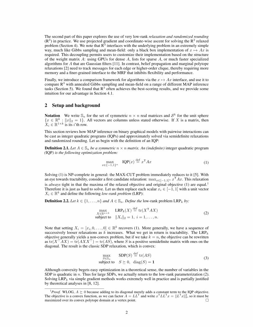
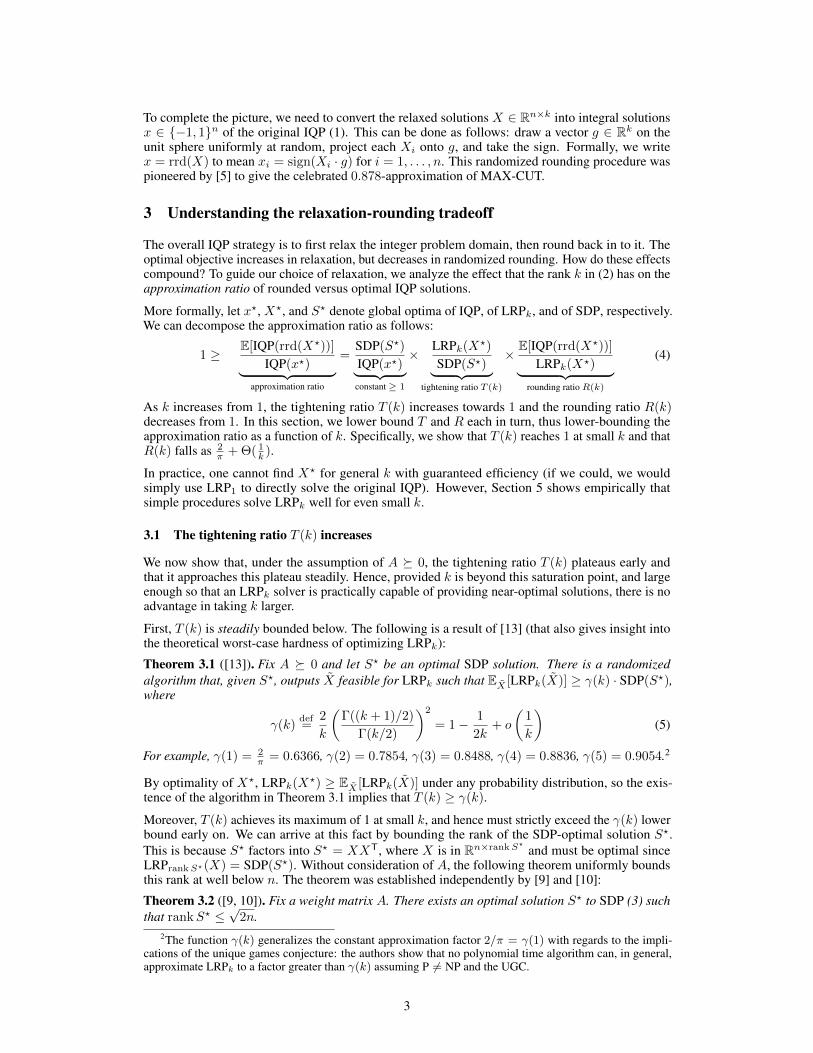
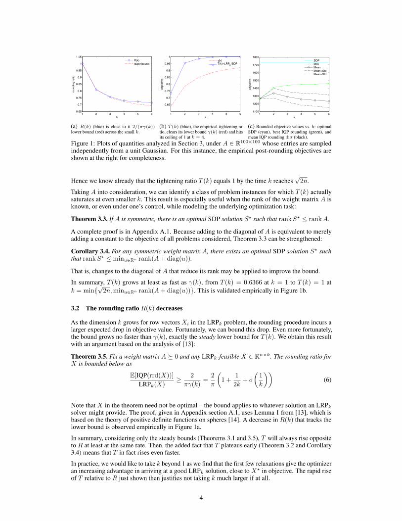
Figure 1: Plots of quantities analyzed in Section 3, under A 2 R100⇥100 whose entries are sampledindependently from a unit Gaussian. For this instance, the empirical post-rounding objectives areshown at the right for completeness.

Hence we know already that the tightening ratio T (k) equals 1 by the time k reachesp

2n.

Taking A into consideration, we can identify a class of problem instances for which T (k) actuallysaturates at even smaller k. This result is especially useful when the rank of the weight matrix A isknown, or even under one’s control, while modeling the underlying optimization task:

Theorem 3.3. If A is symmetric, there is an optimal SDP solution S? such that rank S? rank A.

A complete proof is in Appendix A.1. Because adding to the diagonal of A is equivalent to merelyadding a constant to the objective of all problems considered, Theorem 3.3 can be strengthened:

Corollary 3.4. For any symmetric weight matrix A, there exists an optimal SDP solution S? suchthat rank S? min

u2Rnrank(A + diag(u)).

That is, changes to the diagonal of A that reduce its rank may be applied to improve the bound.

In summary, T (k) grows at least as fast as �(k), from T (k) = 0.6366 at k = 1 to T (k) = 1 atk = min{

p2n, min

u2Rnrank(A + diag(u))}. This is validated empirically in Figure 1b.

3.2 The rounding ratio R(k) decreases

As the dimension k grows for row vectors Xi

in the LRPk

problem, the rounding procedure incurs alarger expected drop in objective value. Fortunately, we can bound this drop. Even more fortunately,the bound grows no faster than �(k), exactly the steady lower bound for T (k). We obtain this resultwith an argument based on the analysis of [13]:

Theorem 3.5. Fix a weight matrix A ⌫ 0 and any LRPk

-feasible X 2 Rn⇥k. The rounding ratio forX is bounded below as

E[IQP(rrd(X))]

LRPk

(X)

� 2

⇡�(k)

=

2

⇡

✓1 +

1

2k+ o

✓1

k

◆◆(6)

Note that X in the theorem need not be optimal – the bound applies to whatever solution an LRPk

solver might provide. The proof, given in Appendix section A.1, uses Lemma 1 from [13], which isbased on the theory of positive definite functions on spheres [14]. A decrease in R(k) that tracks thelower bound is observed empirically in Figure 1a.

In summary, considering only the steady bounds (Theorems 3.1 and 3.5), T will always rise oppositeto R at least at the same rate. Then, the added fact that T plateaus early (Theorem 3.2 and Corollary3.4) means that T in fact rises even faster.

In practice, we would like to take k beyond 1 as we find that the first few relaxations give the optimizeran increasing advantage in arriving at a good LRP

k

solution, close to X? in objective. The rapid riseof T relative to R just shown then justifies not taking k much larger if at all.

4

4 Pairwise MRFs, optimization, and inference alternatives

Having understood theoretically how IQP relates to low-rank relaxations, we now turn to MAPinference and empirical evaluation. We will show that the LRP

k

objective can be optimized viaa simple interface to the underlying MRF. This interface then becomes the basis for (a) a MAPinference algorithm based on very low-rank relaxations, and (b) a comparison to two other basicalgorithms for MAP: Gibbs sampling and mean-field variational inference.

A binary pairwise Markov random field (MRF) models a function h over x 2 {0, 1}n given byh(x) =

Pi

i

(xi

) +

Pi<j

✓i,j

(xi

, xj

), where the i

and ✓i,j

are real-valued functions. The MAPinference problem asks for the variable assignment x? that maximizes the function h. An MRFbeing binary-valued and pairwise allows the arbitrary factor tables

i

and ✓i,j

to be transformedwith straightforward algebra into weights A 2 S

n

for the IQP. For the complete reduction, seeAppendix A.2.

We make Section 3 actionable by defining the randomized relaxation and rounding (R3) algorithm forMAP via low-rank relaxations. The first step of this algorithm involves optimizing LRP

k

(2) whoseweight matrix encodes the MRF. In practice, MRFs usually have special structure, e.g., edge sparsity,factor templates, and Gaussian filters [11]. To develop R3 as a general tool, we provide two interfacesbetween the solver and MRF representation, both of which allow users to exploit special structure.

Left-multiplication (x 7! Ax) Assume a function F that implements left matrix multiplication bythe MRF matrix A. This suffices to compute the gradient of the relaxed objective: r

X

LRPk

(X) =

2AX . We can optimize the relaxation using projected gradient ascent (PGA): alternate betweentaking gradient steps and projecting back onto the feasible set (unit-normalizing the rows X

i

if thenorm exceeds 1); see Algorithm 1. A user supplying a left-multiplication routine can parallelize itsimplementation on a GPU, use sparse linear algebra, or efficiently implement a dense filter.

Row-product ((i, x) 7! Ai

x) If the function F further provides left multiplication by any row ofA, we can optimize LRP

k

with coordinate-wise ascent (BCA). Fixing all but the i’th row of X givesa function linear in X

i

whose optimum is Ai

X normalized to have unit norm.

Left-multiplication is suitable when one expects to parallelize multiplication, or exploit commondense structure as with filters. Row product is suitable when one already expects to compute Axserially. BCA also eliminates the need for the step size scheme in PGA, thus reducing the number ofcalls to the left-multiplication interface if this step size is chosen by line search.

X random initialization in Rk⇥n

for t 1 to T do

if parallel then

X ⇧Sk(X + 2⌘t

AX) // Parallel updateelse

for i 1 to n do

Xi

⇧Sk(hAi

, Xi) // Sweep updatefor j 1 to M do

x(j) sign(Xg), where g is a random vector from unit sphere Sk (normalized Gaussian)Output the x(j) for which the objective (x(j)

)

TAx(j) is largest.Algorithm 1: The full randomized relax-and-round (R3) procedure, given a weight matrix A;⇧Sk(·) is row normalization and ⌘

t

is the step size in the t’th iteration.

4.1 Comparison to Gibbs sampling and mean-field

The R3 algorithm affords a tidy comparison to two other basic MAP algorithms. First, it is iterativeand maintains a constant amount of state per MRF variable (a length k row vector). Using therow-product interface, R3 under BCA sequentially sweeps through and updates each variable’s state(row X

i

) while holding all others fixed. This interface bears a striking resemblance to (annealed)Gibbs sampling and mean-field iterative updates [4, 15], which are popular due to their simplicity.Table 1 shows how both can be implemented via the row-product interface.

5

Algorithm Domain Sweep update Parallel update

Gibbs x 2 {�1, 1}n xi

⇠ ⇧

Z

(exp(Ai

x)) x ⇠ ⇧

Z

(exp(Ax))

Mean-field x 2 [�1, 1]

n xi

tanh(Ai

x) x tanh(Ax)

R3 X 2 (Sk

)

n Xi

⇧Sk(Ai

X) X ⇧Sk(X + 2⌘t

AX)

Table 1: Iterative updates for MAP algorithms that use constant state per MRF variable. ⇧Sk denotes`2 unit-normalization of rows and ⇧

Z

denotes scaling rows so that they sum to 1. The R3 sweepupdate is not a gradient step, but rather the analytic maximum for the i’th row fixing the rest.

x1

1(x1) = x1

x2

2(x2) = x2

10x1x2

A =

1

2

"0 1 1

1 0 10

1 10 0

#

Figure 2: Consider the two variable MRF on the left (with x1, x2 2 {�1, 1} for the factor expressions)and its corresponding matrix A. Note x0 is clamped to 1 as per the reduction (A.2). The optimum isx = [1, 1, 1]

T with a value of xTAx = 12. If Gibbs or LRP1 is initialized at x = [1,�1,�1]

T, theneither one will be unlikely to transition away from its suboptimal objective value of 8 (as flippingonly one of x1 or x2 decreases the objective to �10). Meanwhile, LRP2 succeeds with probability 1over random initializations. Suppose X = [1, 0; X1; X2] with X1 = X2. Then the gradient updateis X1 = ⇧S2

(A1X) = ⇧S2(([1, 0] + 10X1)/2), which always points towards X?

1 = X?

2 = [1, 0]

except in the 0-probability event that X1 = X2 = [�1, 0] (corresponding to the poor initializationof [1,�1,�1]

T above). The gradient with respect to X1 at points along the unit circle is shown onthe right. The thick arrow represents an X1 ⇡ [�0.95, 0.3], and the gradient field shows that it williteratively update towards the optimum.

Using left-multiplication, R3 updates the state of all variables in parallel. Superficially, both Gibbsand the iterative mean-field update can be parallelized in this way as well (Table 1), but doingso incorrectly alters the their convergence properties. Nonetheless, [11] showed that a simplemodification works well in practice for mean-field, so we consider these algorithms for a completecomparison.3

While Gibbs, mean-field, and R3 are similar in form, they differ in their per-variable state: Gibbsmaintains a number in {�1, 1} whereas R3 stores an entire vector in Rk. We can see by examplethat the extra state can help R3 avoid local optima that ensnarls Gibbs. A single coupling edge in atwo-node MRF, described in Figure 2, gives intuition for the advantage of optimizing relaxationsover stochastic hill-climbing.

Another widely-studied family of MAP inference techniques are based on belief propagation orrelaxations of the marginal polytope [4]. For belief propagation, and even for the most basic of theLP relaxations (relaxing to the local consistency polytope), one needs to store state for every edge inaddition to every variable. This demands a more complex interface to the MRF, introduces substantialadded bookkeeping for dense graphs, and is not amenable to techniques such as the filter of [11].

5 Experiments

We compare the algorithms from Table 1 on three benchmark MRFs and an additional artificial MRF.We also show the effect of the relaxation k on the benchmarks in Figure 3.

Rounding in practice The theory of Section 3 provides safeguard guarantees by considering theaverage-case rounding. In practice, we do far better than average since we take several roundings andoutput the best. Similarly, Gibbs’ output is taken as the best along its chain.

Budgets Our goal is to see how efficiently each method utilizes the same fixed budget of queries tothe function, so we fix the number queries to the left-multiplication function F of Section 4. A budgetjointly limits the relaxation updates and the number of random roundings taken in R3. We charge

3Later, in [16], the authors derive the parallel mean-field update as being that of a concave approximation tothe cross-entropy term in the true mean-field objective.

6

algo. dataset [name (# of instances)]seg (50) dbn (108) grid40 (8) chain (300)

low

bu

dg

et

sw

eep Gibbs 8.35 (23) 1.39 (30) 14.5 (7) .473 (37)

MF 8.36 (23) 1.3 (7) 13.6 (1) .463 (39)R3 8.39 (15) 1.42 (71) 13.7 (0) .538 (296)

pa

ra

llel Gibbs 7.4 (19) .826 (3) .843 (0) .124 (3)

MF 7.4 (26) 1.16 (6) 11.3 (3) .35 (50)R3 7.4 (17) 1.29 (99) 11.3 (5) .418 (282)

hig

hb

ud

get

sw

eep Gibbs 7.07 (33) 1.26 (42) 12.5 (7) .367 (85)

MF 7.03 (9) 1.16 (4) 11.7 (1) .33 (39)R3 7.09 (23) 1.28 (62) 11.9 (0) .398 (300)

pa

ra

llel Gibbs 6.78 (31) .814 (2) 1.85 (0) .132 (11)

MF 6.75 (12) 1.1 (2) 10.9 (2) .259 (47)R3 6.8 (25) 1.25 (104) 11 (6) .321 (296)

Table 2: Benchmark performance of algorithms in each comparison regime, in which the benchmarksare held to different computational budgets that cap their access to the left-multiplication routine. Thescore shown is an average relative gain in objective over the uniform-random baseline. Parenthesizedis the win count (including ties), and bold text highlights qualitatively notable successes.

1 2 3 4 5 6460

480

500

520

540

560

580

k

ob

ject

ive

seg

LRPMaxMeanMean+StdMean−Std

1 2 3 4 5 60.95

1

1.05

1.1

1.15

1.2

1.25

1.3x 10

4

k

ob

ject

ive

dbn

LRPMaxMeanMean+StdMean−Std

1 2 3 4 5 61.1

1.15

1.2

1.25

1.3

1.35

1.4x 10

4

k

ob

ject

ive

grid

LRPMaxMeanMean+StdMean−Std

Figure 3: Relaxed and rounded objectives vs. the rank k in an instance of seg, dbn, and grid40. Blue:max of roundings. Red: value of LRP

k

. Black: mean of roundings (±�). The relaxation objectiveincreases with k, suggesting that increasingly good solutions are obtained by increasing k, in spite ofnon-convexity (here we are using parallel updates, i.e. using R3 with PGA). The maximum roundingalso improves considerably with k, especially at first when increasing beyond k = 1.

R3 k-fold per use of F when updating, as it queries F with a k-row argument.4 Sweep methods arecharged once per pass through all variables.

We experiment with separate budgets for the sweep and parallel setup, as sweeps typically convergemore quickly. The benchmark is run under separate low and high budget regimes – the latter morethan double the former to allow for longer-run effects to set in. In Table 2, the sweep algorithms’ lowbudget is 84 queries; the high budget is 200. The parallel low budget is 180; the high budget is 400.We set R3 to take 20 roundings under low budgets and 80 under high ones, and the remaining budgetgoes towards LRP

k

updates.

Datasets Each dataset comprises a family of binary pairwise MRFs. The sets seg, dbn, and grid40

are from the PASCAL 2011 Probabilistic Inference Challenge5 — seg are small segmentation models(50 instances, average 230 variables, 622 edges), dbn are deep belief networks (108 instances, average920 variables, 54160 edges), and grid40 are 40x40 grids (8 instances, 1600 variables, 6240 or 6400edges) whose edge weights outweigh their unaries by an order of magnitude. The chain set comprises300 randomly generated 20-node chain MRFs with no unary potentials and random unit-Gaussianedge weights – it is principally an extension of the coupling two-node example (Figure 2), and servesas a structural obverse to grid40 in that it lacks cycles entirely. Among these, the dbn set comprisesthe largest and most edge-dense instances.

4 This conservatively disfavors R3, as it ignores the possible speedups of treating length-k vectors as a unit.5http://www.cs.huji.ac.il/project/PASCAL/

7

Evaluation To aggregate across instances of a dataset, we measure the average improvement overa simple baseline that, subject to the budget constraint, draws uniformly random vectors in {�1, 1}nand selects the highest-scoring among them. Improvement over the baseline is relative: if z is thesolution objective and z0 is that of the baseline, (z � z0)/z0 is recorded for the average. We alsocount wins (including ties), the number of times a method obtains the best objective among thecompetition. Baseline performance varies with budget so scores are incomparable across sweep andparallel experiments.

In all experiments, we use LRP4, i.e. the width-4 relaxation. The R3 gradient step size scheme is⌘t

= 1/p

t. In the parallel setting, mean-field updates are prone to large oscillations, so we smooththe update with the current point: x (1� ⌘)x + ⌘ tanh(Ax). Our experiments set ⌘ = 0.5. Gibbsis annealed from an initial temperature of 10 down to 0.1. These settings were tuned towards thebenchmarks using a few arbitrary instances from each dataset.

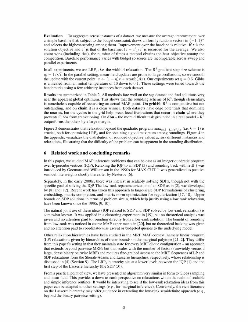
Results are summarized in Table 2. All methods fare well on the seg dataset and find solutions verynear the apparent global optimum. This shows that the rounding scheme of R3, though elementary,is nonetheless capable of recovering an actual MAP point. On grid40, R3 is competitive but notoutstanding, and on chain it is a clear winner. Both datasets have edge potentials that dominatethe unaries, but the cycles in the grid help break local frustrations that occur in chain where theyprevents Gibbs from transitioning. On dbn – the more difficult task grounded in a real model – R3

outperforms the others by a large margin.

Figure 3 demonstrates that relaxation beyond the quadratic program max

x2[�1,1]xTAx

(i.e. k = 1) iscrucial, both for optimizing LRP

k

and for obtaining a good maximum among roundings. Figure 4 inthe appendix visualizes the distribution of rounded objective values across different instances andrelaxations, illustrating that the difficulty of the problem can be apparent in the rounding distribution.

6 Related work and concluding remarks

In this paper, we studied MAP inference problems that can be cast as an integer quadratic programover hypercube vertices (IQP). Relaxing the IQP to an SDP (3) and rounding back with rrd(·) wasintroduced by Goemans and Williamson in the 1990s for MAX-CUT. It was generalized to positivesemidefinite weights shortly thereafter by Nesterov [6].

Separately, in the early 2000s, there was interest in scalably solving SDPs, though not with thespecific goal of solving the IQP. The low-rank reparameterization of an SDP, as in (2), was developedby [8] and [12]. Recent work has taken this approach to large-scale SDP formulations of clustering,embedding, matrix completion, and matrix norm optimization for regularization [17, 18]. Upperbounds on SDP solutions in terms of problem size n, which help justify using a low rank relaxation,have been known since the 1990s [9, 10].

The natural joint use of these ideas (IQP relaxed to SDP and SDP solved by low-rank relaxation) issomewhat known. It was applied in a clustering experiment in [19], but no theoretical analysis wasgiven and no attention paid to rounding directly from a low-rank solution. The benefit of roundingfrom low-rank was noticed in coarse MAP experiments in [20], but no theoretical backing was givenand no attention paid to coordinate-wise ascent or budgeted queries to the underlying model.

Other relaxation hierarchies have been studied in the MRF MAP context, namely linear program(LP) relaxations given by hierarchies of outer bounds on the marginal polytope [21, 2]. They differfrom this paper’s setting in that they maintain state for every MRF clique configuration – an approachthat extends beyond pairwise MRFs but that scales with the number of factors (unwieldy versus alarge, dense binary pairwise MRF) and requires fine-grained access to the MRF. Sequences of LP andSDP relaxations form the Sherali-Adams and Lasserre hierarchies, respectively, whose relationship isdiscussed in [4] (Section 9). The LRP

k

hierarchy sits at a lower level: between the IQP (1) and thefirst step of the Lasserre hierarchy (the SDP (3)).

From a practical point of view, we have presented an algorithm very similar in form to Gibbs samplingand mean-field. This provides a down-to-earth perspective on relaxations within the realm of scalableand simple inference routines. It would be interesting to see if the low-rank relaxation ideas from thispaper can be adapted to other settings (e.g., for marginal inference). Conversely, the rich literatureon the Lasserre hierarchy may offer guidance in extending the low-rank semidefinite approach (e.g.,beyond the binary pairwise setting).

8

References

[1] S. Geman and D. Geman. Stochastic relaxation, Gibbs distributions, and the Bayesian restoration ofimages. IEEE Transactions on Pattern Analysis and Machine Intelligence (PAMI), 6:721–741, 1984.

[2] D. Sontag, T. Meltzer, A. Globerson, Y. Weiss, and T. Jaakkola. Tightening LP relaxations for MAP usingmessage-passing. In Uncertainty in Artificial Intelligence (UAI), pages 503–510, 2008.

[3] A. Rush, D. Sontag, M. Collins, and T. Jaakkola. On dual decomposition and linear programmingrelaxations for natural language processing. In Empirical Methods in Natural Language Processing(EMNLP), pages 1–11, 2010.

[4] M. Wainwright and M. I. Jordan. Graphical models, exponential families, and variational inference.Foundations and Trends in Machine Learning, 1:1–307, 2008.

[5] M. Goemans and D. Williamson. Improved approximation algorithms for maximum cut and satisfiabilityproblems using semidefinite programming. Journal of the ACM (JACM), 42(6):1115–1145, 1995.

[6] Y. Nesterov. Semidefinite relaxation and nonconvex quadratic optimization. Optimization methods andsoftware, 9:141–160, 1998.

[7] N. Alon and A. Naor. Approximating the cut-norm via Grothendieck’s inequality. SIAM Journal onComputing, 35(4):787–803, 2006.

[8] S. Burer and R. Monteiro. A nonlinear programming algorithm for solving semidefinite programs vialow-rank factorization. Mathematical Programming, 95(2):329–357, 2001.

[9] A. I. Barvinok. Problems of distance geometry and convex properties of quadratic maps. Discrete &Computational Geometry, 13:189–202, 1995.

[10] G. Pataki. On the rank of extreme matrices in semidefinite programs and the multiplicity of optimaleigenvalues. Mathematics of Operations Research, 23(2):339–358, 1998.

[11] P. Krahenbuhl and V. Koltun. Efficient inference in fully connected CRFs with Gaussian edge potentials.In Advances in Neural Information Processing Systems (NIPS), 2011.

[12] S. Burer and R. Monteiro. Local minima and convergence in low-rank semidefinite programming. Mathe-matical Programming, 103(3):427–444, 2005.

[13] J. Briet, F. M. d. O. Filho, and F. Vallentin. The positive semidefinite Grothendieck problem with rankconstraint. In Automata, Languages and Programming, pages 31–42, 2010.

[14] I. J. Schoenberg. Positive definite functions on spheres. Duke Mathematical Journal, 9:96–108, 1942.[15] M. I. Jordan, Z. Ghahramani, T. S. Jaakkola, and L. K. Saul. An introduction to variational methods for

graphical models. Machine Learning, 37:183–233, 1999.[16] P. Krahenbuhl and V. Koltun. Parameter learning and convergent inference for dense random fields. In

International Conference on Machine Learning (ICML), pages 513–521, 2013.[17] B. Kulis, A. C. Surendran, and J. C. Platt. Fast low-rank semidefinite programming for embedding and

clustering. In Artificial Intelligence and Statistics (AISTATS), pages 235–242, 2007.[18] B. Recht and C. Re. Parallel stochastic gradient algorithms for large-scale matrix completion. Mathematical

Programming Computation, 5:1–26, 2013.[19] J. Lee, B. Recht, N. Srebro, J. Tropp, and R. Salakhutdinov. Practical large-scale optimization for max-

norm regularization. In Advances in Neural Information Processing Systems (NIPS), pages 1297–1305,2010.

[20] S. Wang, R. Frostig, P. Liang, and C. Manning. Relaxations for inference in restricted Boltzmann machines.In International Conference on Learning Representations (ICLR), 2014.

[21] D. Sontag and T. Jaakkola. New outer bounds on the marginal polytope. In Advances in Neural InformationProcessing Systems (NIPS), pages 1393–1400, 2008.

9

A Appendix

A.1 Proofs

A.1.1 Proof of Theorem 3.3

Proof. For simplicity, we first consider the case of symmetric PSD A. Let k?

= rank A. ConsiderX 2 Rn⇥k with ||X

i

||2 1 and k > k? such that LRPk

(X) = tr(XTAX) attains the optimalvalue of the SDP (this is possible in particular when k = n). We want to to transform X to thethinner X? 2 Rn⇥k

?

that still satisfies the row norm constraints ||X?

i

||2 1. Let Q 2 Rk⇥k be anorthonormal matrix (QQT

= Ik

). Note that XQ still satisfies the row norm constraints (since eachrow of X

i

just gets rotated). Thus, it suffices to find Q so that some columns of XQ fall into thenull-space of A and can be discarded.

Suppose A ⌫ 0. Let A = LLT for L 2 Rn⇥k

?

and let Y = LTX 2 Rk

?⇥k. We can chooseQ so that Y Q 2 Rk

?⇥k has at most k? non-zero columns, i.e. take Q = [Qbasis, Qnull], whereQnull 2 Rk⇥(k�k

?) comprises the k � k? columns such that Y Qnull = 0 and Qbasis 2 Rk⇥k

?

comprises the first k? columns of Q. Obtaining such a Q is possible by taking an orthonormal basisof the null space of Y as the columns of Qnull, and taking an orthonormal basis of the k?-dimensionalrow space of Y as the columns of Qbasis. Both bases can be obtained by applying the Gram-Schmidtprocess.

Now when we transform X by Q to get XQ = [XQbasis, XQnull], we can drop the columns XQnullsince 0 = Y Qnull = LTXQnull, thus removing XQnull does not change the objective. SettingX?

= XQbasis 2 Rn⇥k

?

gives that LRPk

(X?

) = LRPk

(X) and we get the desired rank reductionwithout changing the objective and while maintaining satisfiability of the row norm constraints.

More generally if A is real symmetric (but not necessarily A ⌫ 0) then we can consider instead thefactorization A = LRT where the columns of R are identical to the columns of L except possiblynegated. Such a factorization is given by the eigendecomposition of a real symmetric matrix. In thiscase, Q still rotates both L and R correctly and the above argument follows in the same way.

We remark that even more generally, if A = LUT for L, U 2 Rn⇥k

?

for n � k � 2k?, then we canset Qbasis to be the basis of the row space of Y = [LTX; UTX] 2 R2k?⇥k. Then the same argumentstill applies but we can only reduce the solution rank from k to 2k?

= 2 rank(A).

A.1.2 Proof of Theorem 3.5

Proof. The proof relies on Grothendieck’s identity: if u, v 2 Rk and g is drawn uniformly from theunit sphere Sk, then

E⇥sign(uTg) sign(vTg)

⇤=

2

⇡arcsin(uTv). (7)

Let Y = f(XXT) 2 Rn⇥n be the elementwise application of the scalar function

f(t) =

2⇡

⇣arcsin(t) � t

�(k)

⌘. (8)

Lemma 1 in [13] shows that f(t) is a function of the positive type on Sk, which by definition meansthat Y ⌫ 0 provided X

i

2 Sk for all i. The underlying theory is developed in [14].

For A, Y ⌫ 0 we have that tr(AY ) � 0. Rearranging terms and applying Grothendieck’s identity,

0 tr(AY ) = tr

✓A

2

⇡

✓arcsin(XXT

) � XXT

�(k)

◆◆(9)

() tr

✓A

2

⇡arcsin(XXT

)

◆� 2

⇡�(k)

tr(AXXT) (10)

() E[IQP(rrd(X))] � 2

⇡�(k)

LRPk

(X), (11)

as claimed.

10

A.2 MRF to IQP reduction

Using the shorthand i;u =

i

(u) and ✓ij;uv = ✓

i,j

(u, v), the negative energy can be written as asum of terms

i;1xi

+ i;0(1 � x

i

) and of terms

✓ij;11xi

xj

+ ✓ij;10xi

(1 � xj

) + ✓ij;01(1 � x

i

)xj

+ ✓ij;00(1 � x

i

)(1 � xj

) (12)

for every i, j, i.e. negative energy is a quadratic form over {0, 1}n, and finding its maximum isprecisely the MAP problem. This quadratic form over can be written as xTMx + �Tx + �0, where

Mi,j

def= ✓

ij;11 + ✓ij;00 � ✓

ij;10 � ✓ij;01 for i < j (13)

�i

def=

i;1 � i;0 +

Pj>i

(✓ij;10 � ✓

ij;00) +

Pj<i

(✓ji;01 � ✓

ji;00) for every i (14)

�0def=

Pi

i;0 +

Pi<j

✓ij;00 (15)

This in turn can be written more compactly as xT(M 0

+diag(�))x+�0, where M 0= (M +MT

)/2

is taken for symmetry. In summary, MAP in the MRF reduces to maximizing the term left of �0 (thatwhich we can control), which is now in a form that differs from IQP only by the domain of x.

One can then reduce the problem from the x 2 {0, 1}n domain to x 2 {�1, 1}n by a linear changeof variables. Given an IQP as in (1) with objective xTAx over x 2 {0, 1}n, we can equivalentlyoptimize [

12 (x + 1)]

TA[

12 (x + 1)] over x 2 {�1, 1}n. This reduction introduces cross-terms. Define

bdef= 1TA + A1 = 2A1 2 Rn b0

def= 1TA1 =

121

Tb 2 Rn (16)

Now, optimizing over x 2 {�1, 1}n, we can fold b and b0 into A by introducing a single auxiliaryvariable x0 (so the new domain is x0

= (x0, x)) and augmenting A to

A0=

1

4

b0

12bT

12b A

�. (17)

The variable x0 must be constrained to 1, but in practice such a constraint can be ignored up until weoutput a final solution, because negating all of x has no effect on the IQP objective.

A.3 Additional figures

Figure 4 shows empirical histograms of objectives of random roundings from an LRPk

solution.

Evaluations

Histograms of the rrr-MAP samples vs. k

*

*

*

*

*

*

*

*

**

*

*

Figure : From top to bottom, rows vary across k = 2, 4, 8. From left to right,columns show: (1) random A; (2) a pairwise distance matrix formed by MNISTdigits 4 and 9; (3) an instance from seg; (4) an instance from dbn. The limits ofthe x-axis is identical in each column.

Wang & Frostig (Stanford) Randomized relax-and-round April 15, 2014 23 / 27

k=2$$$$$$$$$$$$$$$$$$$

Random$ Distance$ Seg.$ DBN$

k=4$$$$$$$$$$$$$$$$$$$

k=8$$$$$$$$$$$$$$$$$$$

Figure 4: Distribution of the value of random roundings across problem instances and ranks. Fromtop to bottom, rows vary across k = 2, 4, 8. From left to right, columns show: (1) random A; (2) apairwise distance matrix formed by MNIST digits 4 and 9; (3) an instance from seg; (4) an instancefrom dbn. The range of the x-axis is identical in each column.

11