SIMPLE AND APPROXIMATELY OPTIMALMECHANISMS DESIGN

A Dissertation

Presented to the Faculty of the Graduate School

of Cornell University

in Partial Fulfillment of the Requirements for the Degree of

Doctor of Philosophy

by

Hu Fu

August 2013

c© 2013 Hu Fu

ALL RIGHTS RESERVED

SIMPLE AND APPROXIMATELY OPTIMAL MECHANISMS DESIGN

Hu Fu, Ph.D.

Cornell University 2013

Mechanism design studies optimization problems with inputs from selfishly behaving

agents. To a class of relatively simple questions, classical auction theory gives optimal

solution which are often too complicated for practical use. This dissertation presents

techniques and results on the design and analysis of simple and practical auctions that

have provably approximately optimal performances. For single-parameter revenue op-

timization, we present the k-lookahead auction, which works for coorelated valuation

distributions, and we discuss its consequences, which encompass a family of reserve-

price-based auctions with approximately optimal revenue. For more general settings, we

present the marginal revenue mechanisms as a framework for designing simple mech-

anisms in very general settings. Both frameworks are motivated with clear economic

intuitions.

For social welfare maximization in combinatorial auctions, we present an equilib-

rium analysis for simultaneous item auctions. In particular, we show that when val-

uations exhibit no complements, the welfare loss in these auctions at Bayesian Nash

equilibria is bounded by small constants.

BIOGRAPHICAL SKETCH

Hu Fu was born in Qingdao, China in 1984. Piano practice and performance occupied

much of his childhood and has ever since been a nontrivial diversion. Hu won a gold

medal in the Chinese National Biology Olympiad in 2002, and went on to the Depart-

ment of Automation at Tsinghua University for his college education. There he won

the prestigious Jiang Nanxiang Scholarship in 2004, and obtained his bachelor degree

in 2007. Since then he has been pursuing his graduate study in computer science at

Cornell University.

iii

This dissertation is dedicated to my parents, and to the memory of my grandfather,

Huizan Fu.

iv

ACKNOWLEDGMENTS

It is most certain that the luckiest thing that happened to me in graduate school

was to have found Bobby Kleinberg as my advisor. Not only did Bobby allure me to

the wonderland of theoretical computer science, set me a model of academic brilliancy

brimming with dazzling ideas, and provide crucial help with all my key career decisions,

but also, in the true spirit of academic genealogy, he inculcated in me a taste for research

and mathematics in general, an influence whose effect I expect to perceive for years to

come. It was additional bliss to have Bobby as a genuine friend, to share and play music

and to discuss all intellectual matters with him.

Among the colleagues I have collaborated with, Jason Hartline and Shahar Dobzin-

ski have virtually come to assume the role of second advisors. I owe to them the inspira-

tion of some of my best research outputs, and have repeatedly benefited from their wise

advice.

I was born into a family whose intellectual tradition was disrupted for a generation

by social upheavals. Fostering my intellectual growth therefore exacts additional sacri-

fice and patience from my parents, for which I am forever grateful. My grandparents,

especially my late grandfather, sowed in me the scholarly seed. Under their and my

parents’ care, it budded through hardships not easily conceived in this country, and is

now finally bearing some flowers. To think of the joy and pride this brings to them

emboldens me before all obstacles in life.

The way I think about math was greatly changed and ripened by courses I took from

Eugene Dynkin and Ken Brown. My enjoyment in graduate school was enriched by

piano lessons taken from Xak Bjerken, and my intellectual horizon was tremendously

broadened by my three years of residence in the Telluride House. Friendships I formed

in the Computer Science Department and at the Telluride House, such as those with

Thanh Nguyen, Tuan Cao, Huijia Lin, Chenhao Tan, Hussam Abu-Libdeh, Judah Bellin,

v

Kate Scheibel, Liz Solten, Sarah Asman, Jacob Krell and Srinath Reddy, are cherished

in memory and will for sure be a lifelong treasure.

vi

TABLE OF CONTENTS

Biographical Sketch . . . . . . . . . . . . . . . . . . . . . . . . . . . . . . . iiiDedication . . . . . . . . . . . . . . . . . . . . . . . . . . . . . . . . . . . . ivAcknowledgments . . . . . . . . . . . . . . . . . . . . . . . . . . . . . . . . vTable of Contents . . . . . . . . . . . . . . . . . . . . . . . . . . . . . . . . vii

1 Introduction 11.1 (Approximately) Optimal Auctions Beyond Myerson. . . . . . . . . . . 21.2 Towards More Realistic Mechanisms . . . . . . . . . . . . . . . . . . . 41.3 Bibliographic Notes . . . . . . . . . . . . . . . . . . . . . . . . . . . . 5

2 Background Material 6

3 Lookahead Auctions and Their Consequences 113.1 Preliminary . . . . . . . . . . . . . . . . . . . . . . . . . . . . . . . . 113.2 The k-lookahead Auction . . . . . . . . . . . . . . . . . . . . . . . . . 12

3.2.1 Analysis of the k-Lookahead Auction . . . . . . . . . . . . . . 133.3 Reserve-price-based Auctions for Independent Distributions . . . . . . 17

3.3.1 Preliminaries . . . . . . . . . . . . . . . . . . . . . . . . . . . 183.3.2 Single Item Settings . . . . . . . . . . . . . . . . . . . . . . . 203.3.3 Matroid Settings . . . . . . . . . . . . . . . . . . . . . . . . . 23

4 Marginal Revenue Mechanisms 294.1 Introduction . . . . . . . . . . . . . . . . . . . . . . . . . . . . . . . . 294.2 Warmup: Single-dimensional Linear Preference . . . . . . . . . . . . . 384.3 Multi-dimensional and Nonlinear Preferences . . . . . . . . . . . . . . 444.4 Implementation . . . . . . . . . . . . . . . . . . . . . . . . . . . . . . 53

4.4.1 Monotone Ex Ante Constrained Lottery Pricings . . . . . . . . 544.4.2 General Ex Ante Constrained Lottery Pricings . . . . . . . . . 56

4.5 Approximation . . . . . . . . . . . . . . . . . . . . . . . . . . . . . . 574.5.1 Agent-based Approximation . . . . . . . . . . . . . . . . . . . 574.5.2 Feasibility-based Approximation . . . . . . . . . . . . . . . . . 62

4.6 Extending Techniques From Single-Dimensional Linear Utility Settings 66

5 Simultaenous Item Auctions 685.1 Introduction . . . . . . . . . . . . . . . . . . . . . . . . . . . . . . . . 685.2 Preliminaries . . . . . . . . . . . . . . . . . . . . . . . . . . . . . . . 75

5.2.1 Combinatorial Auctions and Equilibria . . . . . . . . . . . . . 755.2.2 Subadditive Valuations . . . . . . . . . . . . . . . . . . . . . . 785.2.3 Overbidding . . . . . . . . . . . . . . . . . . . . . . . . . . . 80

5.3 Bidding Under Uncertain Prices . . . . . . . . . . . . . . . . . . . . . 805.4 BPoA of First Price Auctions . . . . . . . . . . . . . . . . . . . . . . . 845.5 BPoA of Second Price Auctions . . . . . . . . . . . . . . . . . . . . . 87

vii

A Proofs from Chapter 4 90A.1 Single-dimensional Proofs . . . . . . . . . . . . . . . . . . . . . . . . 90A.2 Proofs from Section 4.3 . . . . . . . . . . . . . . . . . . . . . . . . . . 91A.3 Linearity . . . . . . . . . . . . . . . . . . . . . . . . . . . . . . . . . . 93A.4 Proofs from Section 4.4.2 . . . . . . . . . . . . . . . . . . . . . . . . . 95A.5 Proofs for unit-demand approximation . . . . . . . . . . . . . . . . . . 98

viii

CHAPTER 1

INTRODUCTION

Mechanism design studies optimization systems that take into account participants’

private information and selfish behaviors. The past ten years have seen a fruitful mar-

riage of this subfield of microeconomics with computer science, accelerated by the ad-

vent of the Internet and the ensuing business on it, such as display ad auctions run by

search engine companies and large scale, dynamic auctions run by websites like Price-

line or eBay. Algorithmic ideas and tools have been brought to bear on decades-old

problems of economic theory, yielding new economic insights in addition to potential

impacts on industries.

This thesis focuses on two aspects of this development. First, economic characteri-

zations of optimal mechanisms beyond classic scenarios tend to be too complex for prac-

tical use. A theme of the chapters to follow to that, when the viewpoint of approximation

is adopted, much more structure and insights can be revealed and applied. Second, and

relatedly, the use of mechanisms in practice often favors simplicity over theoretical op-

timality, when the two design goals come into conflict. Simplicity here may refer to

systems having succinct specifications, requiring less self-deliberation and private in-

formation disclosure by market participants, tolerating the lack of certain information

on the mechanism implementer’s part, and so on. This thesis presents research progress

showing, on one hand, that the structure gained from adopting approximations often

guides the design of simple mechanisms, and on the other hand, that mechanisms used

in practice can often be analyzed and evaluated as approximations to optimal bench-

marks.

Background. A mechanism involves the participation of strategic agents with private

information. The agents’ information, summarized as types, is unknown to us, while

a decision on a social outcome needs to be made from interactions with them. In an

1

auction, for example, a bidder’s type may describe her valuations of the items being

sold, and the social outcome is a decision to sell which items to which bidders at what

prices. The mechanism designer devises rules of interaction and decision, so that certain

goals, usually functions of the agents’ types, can be optimized, while taking heed that

the agents may behave strategically—their interests, expressed in utilities, are typically

affected by the social outcome. A bedrock solution concept in mechanism design is in-

centive compatibility in direct revelation mechanisms. In a direct revelation mechanism,

each agent reports her type to the mechanism; the mechanism is said to be incentive

compatible if all agents of all types find it in their best interests to reveal information

honestly. On this solution concept stand two Nobel-prize-winning works. One is the

Vickrey-Clark-Groves (VCG) mechanism [18, 28, 54], a general procedure maximizing

the social welfare (the sum of all participants’ utilities). The other is Myerson’s auc-

tion that optimizes the seller’s expected revenue [43]. These two mechanisms bolster a

large part of the study of mechanism design, but beyond very simple settings they either

cannot be generalized or have too complex (economically or computationally or both)

generalizations to be practical. A recurring theme of this thesis is to restore simplicity

to these scenarios by way of adopting a viewpoint of approximations.

1.1 (Approximately) Optimal Auctions Beyond Myerson.

The optimal auction by Myerson maximizes the seller’s expected revenue for bidders

with linear utilities and independently drawn valuations. (An agent is said to have lin-

ear utility if her utility is equal to her value of the service or items she gets minus the

payment she makes.) Notwithstanding its elegance, Myerson’s auction has several limi-

tations. First, unlike auctions commonly run in practice, where the outcome is typically

transparently decided by comparisons among the bidders’ bids above reserve prices,

Myerson’s auction is relatively complicated. One manifestation of this complexity is

2

that a bidder with a lower bid can at times win over higher bidders. Second, when bid-

ders’ valuations are correlated, its revenue can be far from optimal [43]. Third, Myer-

son’s optimal auction does not generalize to settings where bidders have multi-parameter

types or non-linear utilities.

In Chapter 3 we investigate the first two limitations. A formally simple solution

to the correlated distribution cases turns out to be instrumental with developing sim-

ple approximations in the independent value case. We start with the following simple

k-lookahead auction, generalizing the lookahead auction proposed by Ronen [48]: con-

ditioning on lower bids, run the optimal auction on the highest k bidders. We show

the revenue of this auction to be at least 2k−13k−1 of the optimal revenue extractable if we

require that a truthful bidder never ends up with a negative utility. This result quan-

tifies the importance of high bidders in terms of approximations. Lookahead auctions

were originally developed for correlated valuations, but their analysis sheds light on

reserve-price-based practical auctions under independent valuations. In the second part

of Chapter 3, we present several such auctions with approximately optimal performance

that are simpler than the optimal auctions in various aspects. We note that the latter

results were known prior to this work and were the content of several papers [4, 21, 32],

but the perspective of lookahead auctions allow great simplification of their analysis and

allow us to present all of them rather compactly.

Myerson’s requirement for single-parameter types and linear utilities significantly

restricts the auction’s applicability. For example, multi-item auctions generally require

more than one parameter to describe bidders’ valuations, and bidders that have bud-

gets or are averse to risks cannot be modeled with linear utilities. Recently, a generic

polynomial-time reduction was discovered [1, 11, 12, 13] from the problem of multi-

agent optimal mechanism design to that of single-agent mechanism design. These algo-

rithms are based on convex programming techniques, and produce complex procedures

3

that are neither practical to run nor conducive to economic intuition. In Chapter 4,

we present a framework for searching and analyzing simple and near-optimal mecha-

nisms in these general environments. In a classical paper [9], Bulow and Roberts gave

a simple interpretation of Myerson’s optimal auction: if we see each bidder as a market

wherein the makeup of customers is specified by the distribution of the bidder’s types,

then a monopoly price setter observes a shrinking fraction of buying customers as the

price rises. When optimizing revenue with a limited supply over multiple markets, the

monopolizer rations the supply across the markets by maximizing the sum of marginal

revenues. Myerson’s optimal auction turns out to be the same procedure, by mapping

each type to the marginal revenue corresponding to that customer’s critical buying price.

This simple economics does not generalize to more complex settings, because there is

no obvious mapping from a type to a marginal revenue, and because the mechanism de-

signer has more freedom than simply setting prices in markets.1 We develop techniques

to connect both broken links, first by giving substance to marginal revenue maximization

in general contexts, and second by showing that the procedure achieves approximately

optimal revenue. Such mechanisms provide new insights on the economic structure of

optimal mechanisms beyond Myerson’s setting and have broad potential applications.

One example we give is a simple, near-optimal auction for budgeted bidders in very

general environments.

1.2 Towards More Realistic Mechanisms

Mechanisms used in reality are often not direct revelation incentive compatible but are

simple procedures in which agents have room for strategic behaviors. Such mechanisms

are popular for various reasons. For example, the communication between participants

1Such freedom happens not to render additional power in the single-parameter, linear utility case,which is the key to the relative straightforwardness of the analysis for these cases.

4

in such auctions can be significantly less than a full description of their types. The Gen-

eralized Second Price Auctions (GSP) run by search engines and the auctions on eBay

are examples of such non-incentive-compatible auctions. As these auctions are often

designed based on heuristics, it is of both theoretical and practical interest to analyze

their performance at equilibrium reached by strategic participants.

As an example, we consider combinatorial auctions: m items are sold to n bidders,

where each bidder has a valuation for every possible subset of items, and we would like

to maximize the social welfare. A salient example of this is the auction held by the

Federal Communications Commission (FCC) that sells spectrum to wireless communi-

cation companies. Instead of eliciting combinatorial preferences from participants, it is

much more practical to simultaneously run first- or second-price auctions on the items

separately. (In fact, such auctions are often used in practice; the auctions on eBay can be

seen as an example after reasonable simplification.) Such simultaneous auctions form

games where truthfully bidding one’s valuation on each item can be a very poor strat-

egy, and (Bayesian) Nash equilibrium is an appropriate concept with which to predict

and evaluate the auctions’ outcome. In Chapter 5 we show that, for simultaneous first-

price (and second-price) auctions with complement-free valuations, the social welfare at

any Bayesian Nash equilibrium is at least a half (and a quarter) of the optimal allocation.

1.3 Bibliographic Notes

The material in Section 3.2 is from joint work with Shahar Dobzinski and Bobby Klein-

berg which appeared in [22], and the other parts of Chapter 3 are based on [26]. Chap-

ter 4 is based on joint work with Saeed Alaei, Nima Haghpanah and Jason Hartline

which will appear in [2]. Chapter 5 is based on joint work with Michal Feldman, Nick

Gravin and Brendan Lucier, which appeared in [25].

5

CHAPTER 2

BACKGROUND MATERIAL

In this chapter we give basic definitions in mechanism design, introduce notations to

be used throughout the rest of the thesis, and review a few classical results.

Single-Dimensional Mechanism Design For most of the thesis we will consider

single-dimensional mechanism design problems. In Section 4.3 and Chapter 5 we

will consider multi-dimensional settings. Notations and backgrounds will be provided

therein.

In a single-dimensional auction environment, an auctioneer provides a service to a

set N of n bidders, but with certain constraints on which subsets of bidders he could

simultaneously serve. Formally, if we use [n] to denote the set of bidders, then there is

a set I ⊆ 2[n], such that the auctioneer can serve a subset S of bidders simultaneously if

and only if S is in I. For example, in a single item auction, I consists of all singleton

subsets of [n]. When I forms a matroid on [n], we call the environment a matroid

setting. Matroid settings encompass important types of markets, e.g. digital goods (when

all subsets are feasible, i.e., I = 2[n]), k unit auctions (when I contains all subsets of size

at most k, i.e., is the k-uniform matroid), and unit-demand bipartite matching markets

(when I is a traversal matroid). We say the environment is downward closed if T ∈ I

implies S ∈ I, ∀S ⊆ T .

Valuations and Their Distributions Each bidder i has a private valuation vi for being

served. We will assume that vi is drawn from a distribution whose cumulative distri-

bution function is Fi, i.e., Fi(v) = Pr[vi ≤ v]. The corresponding density function is

denoted as fi. When the valuations of different bidders are independent random vari-

ables, we say they are independent bidders; otherwise they are correlated. The joint

distribution of all bidders’ values is denoted by F. Except for the part on the revenue

guarantee of lookahead auctions (Section 3.2 and relavant theorems in Section 3.3) , we

6

focus on auctions with independent bidders in this thesis. When all bidders’ valuations

are identically independently distributed (i.i.d.), we say they are symmetric; otherwise

they are asymmetric. A standard shortened notation for (v1, . . . , vi−1, v′i , vi+1, . . . , vn) is

(v′i , v−i).

Auctions and Incentive Compatibility An auction is a pair of vector functions (x, p)

defined on tuples of valutions. At the valuations (v1, . . . , vn), the allocation func-

tion, xi(v1, . . . , vn), gives the probability with which bidder i receives the service, and

pi(v1, . . . , vn) , the payment function, denotes the expected payment bidder i makes to

the auctioneer. Bidder i is said to have linear utility, or, equivalently, risk averse, if

his utility in participating the auction (x, p), given the other bidders’ valuations v−i, is

vixi(vi, v−i)−pi(vi, v−i). We will consider risk neutral bidders throughout the thesis except

in Section 4.3.

Since bidders’ valuations are private and their utility is affected by the auction out-

come, which in turn depends on the bidders’ behaviors, the bidders may misreport their

valuations to gain advantage. In order to incentivize truthful behavior, we study auctions

that are incentive compatible. An auction is called dominant strategy incentive compati-

ble (DSIC) or, equivalently, ex post incentive compatible, if, for all (v1, . . . , vn), all i and

all v′i ,

vixi(vi, v−i) − pi(vi, v−i) ≥ vix(v′i , v−i) − pi(v′i , v−i).

An auction is called Bayesian incentive compatible (BIC) if, for all i, vi and v′i ,

Ev−i∼F−i | vi

[vixi(vi, v−i) − pi(vi, v−i)

]≥ Ev−i∼F−i | vi

[vixi(v′i , v−i) − pi(v′i , v−i)

],

where F−i | vi is the conditional distribution of v−i given vi. When the bidders are inde-

pendent, this is just∏

j,i F j.

An auction is said to be ex post individually rational (ex post IR) if, for all (v1, . . . , vn)

7

and all i,

vixi(vi, v−i) − pi(vi, v−i) ≥ 0.

Similarly to the definition of BIC, we say that a mechanism is interim individually ra-

tional (interim IR), if for all i and vi,

Ev−i∼F−i | vi

[vixi(vi, v−i) − pi(vi, v−i)

]≥ 0.

In this thesis we will focus on incentive compatible auctions in Chapter 3 and Chap-

ter 4, where we will use the terms bids and valuations interchangeably. In Chapter 5 we

will consider two auctions that are not incentive compatible.

The social welfare for serving a set S of bidders is∑

i∈S vi. The expected revenue

made by an auction is E(v1,...,vn)∼F[∑

i pi(v1, . . . , vn)].

Characterization of BIC Mechanisms and Optimal Auctions In a seminal work,

Myerson [43] gives a characterization of all BIC mechanisms in single-dimensional

environments with risk-neutral bidders, and also derives the revenue-optimal auction.

These results are summarized in the following theorem, where part 4 is a corollary on

single-item auctions by applying the other parts:

Theorem 2.0.1 (43). For risk-neutral bidders with valuations drawn independently and

identically from F,

1. (monotonicity) The allocation rule x(v) for each agent is monotone non-

decreasing in v.

2. (payment identity) The payment rule satisfies p(v) = vx(v) −∫ v

0x(z)dz.

3. (virtual value) The ex ante expected payment of an agent is Ev[p(v)] =

Ev[ϕ(v)x(v)] where ϕ(v) = v − 1−F(v)f (v) is the virtual value for value v.

4. (optimality) In a single-item auction, when the distribution F is regular, i.e., ϕ(v)

is monotone, the second-price auction with reserve ϕ−1(0) is revenue-optimal.

8

Revenue Curves and Monopoly Reserves One way to interpret Myerson [43]’s char-

acterization is by way of revenue curves. We will repeated make use of this; in fact,

Chapter 4 is virtually devoted to a reinterpretation and generalization of this important

perspective.

Consider selling to a single bidder i by setting a take-it-or-leave-it price. For each

price p, the probability that the bidder takes the price is q = 1 − F(p), and the expected

revenue is p(1 − F(p)). Conversely, for each probability q of selling, the expected

revenue from setting the corresponding price is q · F−1(1 − q). The revenue curve for a

valuation distribution is the plot of this expected revenue against q ∈ [0, 1]. The price

corresponding to the highest point of the revenue curve is called the monopoly reserve

price, denoted by rmon. 1 A consequence of Theorem 2.0.1 is that the optimal auction for

selling to a single bidder is to set the monopoly reserve as the take-it-or-leave-it price.

Importantly, the derivative of the revenue curve at a quantile q is equal to the virtual

value at the corresponding quantile ϕ(F−1(q)) (we will explain this in more detail in

Chapter 4). Therefore, the condition that ϕ(v) is a monotone increasing function (i.e.,

that F is a regular distribution), is equivalent to the condition that the revenue curve

should be concave.

VCG auctions with eager and lazy reserve prices Another classic auction which lies

at the foundation of much work on mechanism design is the VCG auction [54, 18, 28].

In the VCG auction, the winners are the set of bidders that achieves the maximum sum of

valuations over all feasible sets, and each of them pays the critical valuation below which

he would drop from the winning set. Formally, the set W of winners is argmaxS∈I∑

i∈S vi,

and the payment made by a bidder in W is pVCGi = infvi | i ∈ argmaxS∈I

∑j∈S v j.

This payment pVCGi is called the VCG payment or VCG threshold for bidder i. It is a

1When there are multiple prices that maximize the revenue, we always pick the highest price amongthem (corresponding to the lowest q) as the monopoly reserve price, throughout the thesis.

9

quantity defined solely by the valuations of other bidders and the feasibility system I,

and therefore is well defined for all bidders, including those who lose the auction. For

each bidder, the VCG threshold is the value above which he will win the auction, and

below which he loses. Another interpretation of the VCG payment that we will use in

Section 3.3.3 is that it represents the externality of a winner imposed on the rest of the

bidders, i.e., for a winner i, pVCGi is the decrease in welfare among all other bidders

caused by bidder i’s presence.

Two important facts about VCG auctions are that they are dominant strategy in-

centive compatible and they maximize the social welfare. A special case of the VCG

auction is the second-price single-item auction, where the highest bidder wins the item

and pays the second highest bid.

10

CHAPTER 3

LOOKAHEAD AUCTIONS AND THEIR CONSEQUENCES

In this chapter we start by considering the problem of revenue maximization in a

single-item auction with bidders having correlated valuations, under the constraints of

dominant strategy incentive compatibility and ex post individual rationality. A simple

and elegant solution to this problem is the lookahead auction proposed by Ronen [48],

who showed that it gives a 2-approximation to the optimal revenue. In Section 3.2,

we present a generalization, the k-lookahead auctions, which we show gives a 3k−12k−1 -

approximation to the optimal revenue. Then in Section 3.3 we use the idea of the looka-

head auction to study reserve-price-based auctions, which are much simpler and more

commonly used than Myerson’s optimal auctions. Using lookahead auctions, we give

simple proofs for the approximation guarantees of several such auctions.

3.1 Preliminary

For bidders having correlated valuations, Cremer and McLean [19] showed that, for

distributions that satisfy a certain “correlation condition”, one can extract full social

surplus by a DSIC but interim IR auction. In such an auction, the expected revenue

is equal to the expected optimal social welfare, the maximum revenue one can hope

for. However, it is crucial that the mechanism is interim IR only, and not ex post IR,

as the mechanism can sometimes, depending on the value profiles, even charge a large

amount from a bidder who does not win the item. When this is undesirable, as for

example when a bidder has a budget that prevents her from paying more than her value

of an outcome, ex post IR is a more realistic requirement. While the optimal auction

in this case for two bidders is completely solved [45, 22], it is known that computing

the optimal deterministic auction for at least three bidders is NP-hard [45], and the only

known algorithm for computing the optimal randomized mechanism is LP-based, with

11

a running time exponential in n in the worst case [22]. In Section 3.2 we present an ex

post IR auction that approximates the optimal revenue of any randomized mechanism.

The auction is a generalization of the following simple auction proposed by Ronen

[48] which he called the lookahead auction: choose the highest bidder as the tentative

winner; run an optimal auction for the highest bidder on a conditional distribution of his

valuation, where the conditioning is on all other bidders’ valuations and the fact that this

tentative winner’s valuation is above all others’. It is not hard to see that the lookahead

auction is dominant strategy incentive compabible.

Theorem 3.1.1 (48). The lookahead auction gives at least half of the optimal revenue

in a single item auction, even for bidders with correlated valuations.

Ronen’s proof is elementary, and it is instructive to repeat it here for the purpose

of our generalization in Theorem 3.3.8. The revenue from any auction consists of two

parts: H, the revenue extracted from the highest bidder; and L, the revenue extracted

from the rest of the bidders. Since lookahead always runs the optimal auction for the

highest bidder with all the information present, its revenue is at least H. One way to run

the auction for the highest bidder is simply to charge him the second highest valuation,

which is an upper bound on L. Therefore the lookahead auction’s revenue is no less than

both H and L, and hence gets at least half of the optimal revenue.

3.2 The k-lookahead Auction

In this section we generalize the lookahead auction and analyze the k-lookahead auction

defined as follows. Find the k bidders with the highest values, and denote this set of

bidders by K. Run the revenue-maximizing truthful auction for K conditioned on the

values of bidders in N \ K and the fact that all of the bidders in K have valuations than

those in N \ K. Notice that the auction for K can either be the optimal truthful-in-

12

expectation mechanism or the optimal deterministic mechanism.

Theorem 3.2.1. The approximation ratio of the k-lookahead auction is at least 3k−12k−1 . In

particular, for k = 2 the approximation ratio is at least as good as 53 , and the approxi-

mation ratio is bounded above by 32 as k tends to infinity.

3.2.1 Analysis of the k-Lookahead Auction

Denote the original distribution by D, and denote by DK the conditional distribution

of the values of the bidders in K given the values of bidders in N \ K and the fact that

bidders in K all have higher valuations than those in N \ K. We let vk+1 denote the the

value of the (k + 1)th-highest bidder. We show that one of the following three families

of auctions provides a good approximation ratio. The k-lookahead auction obviously

provides at least as much expected revenue, and the theorem follows. The auctions are

defined for k ≥ 2. The second and third auctions depend on a parameter t ≥ 1, to be

specified later.

1. k-Highest Auction: Run the optimal auction. If one of the bidders in N \ K is

assigned the item in the optimal auction, no bidder is assigned the item and no

one is charged anything. If one of the bidders in K is assigned the item in the

revenue-maximizing auction then assign him the item and charge him as in the

revenue-maximizing auction.

2. t-Fixed Price Auction: Select one bidder (“the reserve bidder”) from K uniformly

at random, denote this bidder by i. If any of the bidders in K \ i has value above

t · vk+1 then he receives the item and pays t · vk+1. If there are several such bidders,

break ties arbitrarily. Otherwise, the reserve bidder gets the item and pays vk+1.

3. t-Pivot Auction: Select one bidder (“the pivot”) from K uniformly at random, and

denote this bidder by i. If any of the bidders of in K\i has value above t ·vk+1 then

13

run the revenue maximizing auction for bidders in K, conditioned on the values

of bidders in N \ K and the fact that all bidders in K have higher valuations than

those in N \ K. Otherwise the pivot bidder gets the item and pays vk+1.

It is straightforward to see that the k-Highest Auction and the t-Fixed Price Auction

are truthful and individually rational1. To see that the t-Pivot Auction is truthful we

observe that this auction is monotone: the only non-straightforward case to check is

when a bidder j other than i raises his value and forces the mechanism to run the optimal

auction. However, in this case bidder j was not allocated the item before raising his

value, so monotonicity is preserved.

Proof of Theorem 3.2.1. Throughout this proof, we condition on a fixed valuation pro-

file on N \K. We show that the conditional expected revenue from the k-lookahead auc-

tion approximates the conditional expected revenue from the optimal auction, and there-

fore its expected revenue regardless of the conditioning is still a 3k−12k−1 -approximation.

Let l be the event where no bidder in K has value at least t · vk+1, and let l be the

complement of this event. We partition the expected revenue of the optimal auction:

• let Ll be the expected revenue from bidders in N \ K from instances where event l

occurs.

• let Ll be the expected revenue from bidders in N \ K from instances where event l

occurs.

• Let M be the expected revenue from bidders in K from instances where event l

occurs.

• Let H be the expected revenue from bidders in K from instances where event l

occurs.1If the optimal auctions used by the k-Highest Auction and the t-Pivot Auction are deterministic or

universally truthful, then all three auctions are universally truthful, as is their convex combination. Inthis case our proof shows that there is a deterministic auction on the k highest bidders that achieves a(

3k−12k−1

)-approximation to the deterministic optimal auction.

14

Observe that the expected revenue of the optimal auction is Ll + Ll + H + M. We

continue by proving several lemmas.

Lemma 3.2.2. The expected revenue of the k-Highest Auction is M + H.

Proof. By definition the auction extracts exactly the same revenue as the optimal auction

from bidders in K and no revenue from bidders in N \ K. The lemma follows.

Lemma 3.2.3. The expected revenue of the t-Fixed Price Auction is at least Ll + Mt +

k−1k · t · Ll + 1

k · Ll.

Proof. First, notice that the revenue of the t-Fixed Price Auction in every instance is at

least vk+1 (either the reserve bidder is allocated the item and pays vk+1 or the auction sells

the item at a higher price). Suppose that event l occurs. This case contributes Ll + M to

the expected revenue of the optimal auction. Observe that, if l occurs, in any instance

where the optimal auction sells the item to bidders in N \ K, its revenue is at most vk+1

(the price for a sold item is at most the value of the bidder), and that in any instance the

optimal auction sells the item to bidders in N \K the revenue is at most t ·vk+1. Thus, the

instances where event l occurs contribute Ll + Mt to the expected revenue of the t-Fixed

Price Auction.

Suppose now that event l occurs. Thus, there exists some bidder b with vb > t · vk+1.

With probability exactly k−1k , b is not the reserve bidder and in this case the revenue

of the auction is t · vk+1. With probability 1k we have that b is the reserve bidder and

the revenue of the auction is at least vk+1. In particular, for every instance where the

optimal auction sells the item to bidders in N \ K (at a price of at most vk+1) the t-Fixed

Price Auction has an expected revenue of at least k−1k · t · Ll + 1

k · Ll. Together with the

contribution from instances where event l occurs we have that the expected revenue of

the auction is at least Ll + Mt + k−1

k · t · Ll + 1k · Ll.

Lemma 3.2.4. The expected revenue of the t-Pivot Auction is at least Ll+Mt + k−1

k H+ 1k Ll.

15

Proof. Suppose that event l occurs. The revenue of the t-Pivot Auction in every instance

where l occurs is vk+1. The expected revenue of the optimal auction in this case is Ll +M,

and similarly to the the analysis of the t-Fixed Price Auction the expected contribution

to the revenue from instances where event l occurs is Ll + Mt .

Suppose that event l occurs. Thus, there exists some bidder b with vb > t · vk+1.

With probability exactly k−1k , b is not the reserve bidder and in this case the revenue of

the auction is at least H. With probability 1k we have that b is the reserve bidder and

the revenue of the auction is at least 1k · vk+1. Again, similarly to the analysis of the t-

Fixed Price Auction the expected contribution to the revenue when the event l occurs is

k−1k H+ 1

k Ll. Overall, the expected revenue of the auction is at least Ll+Mt + k−1

k H+ 1k Ll.

Next we need some definitions. Conditioned on the values of bidders in N \ K,

let OPT be the revenue of the revenue-maximizing auction, Rh be the revenue of the

k-Highest Auction, R f be the expected revenue of the t-Fixed Price Auction, Rp the

expected revenue of the t-Pivot Auction and R = max(R f ,Rp). In addition, for the rest

of the proof we fix t = 2k−1k−1 .

Lemma 3.2.5. R ≥ Ll + Ll + H+Mt .

Proof. We divide the analysis into two cases. Suppose first that Ll · t ≥ H, which implies

that k−1k · (t − 1) · Ll = Ll ≥

Ht by our choice of t. We have that:

R f ≥ Ll +Mt

+k − 1

k· t · Ll +

1k· Ll ≥ Ll +

Mt

+ Ll +k − 1

k· (t− 1) · Ll ≥ Ll + Ll +

H + Mt

Suppose now that Ll · t < H:

Rp ≥ Ll+Mt

+k − 1

k·H+

1k·Ll ≥ Ll+

Mt

+Ht

+k2 − 2k + 1k(2k − 1)

·H+1k·Ll > Ll+

Mt

+Ht

+k − 1

k·Ll+

1k·Ll

= Ll + Ll +H + M

t

16

We are now finally able to analyze the ratio between the expected revenue of the

revenue-maximizing auction and the k-lookahead auction. We consider two cases and

show that in each one the expected ratio is at most 2 − 1t = 3k−1

2k−1 . In the first case we

assume that Ll + Ll ≤ (H + M)(1 − 1t ). Therefore,

OPTRh≤

Ll + Ll + H + MH + M

≤(H + M)(1 − 1

t ) + H + MH + M

= 2 −1t

Now assume that Ll + Ll > (H + M)(1 − 1t ). We have that, using Lemma 3.2.5:

OPTR≤

Ll + Ll + H + M

Ll + Ll + H+Mt

<(H + M)(1 − 1

t ) + H + M

(H + M)(1 − 1t ) + H+M

t

= 2 −1t.

3.3 Reserve-price-based Auctions for Independent Distributions

The lookahead auction was developed as a mechanism to approximate optimal revenue

under correlated distributions. However, in this section, we will see that it is powerful

in analyzing reserve-based variants of the VCG auction. These auctions allocate the

item(s) in a manner that maximizes the social welfare, except that the bidders’ values

have to be above a certain threshold called the reserve price2. These auctions are proba-

bly the most ubiquitous in practice, at least much more common than the optimal auction

given by Myerson [43] (Theorem 2.0.1). Hartline and Roughgarden [32] pioneered the

study of revenue guarantees of such auctions. It is reassuring that under fairly general

assumptions such auctions are shown to generate near-optimal revenues.

As indicated below, most results on reserve-based auctions shown in this section

are rederivations of previously known theorems from Hartline and Roughgarden [32],

Dhangwatnotai et al. [21] and Azar et al. [4]. The main contribution of this section is

2When the same reserve price is used for all bidders, it can be interpreted as the value of the auctioneerfor the item being auctioned, and the VCG auction with a reserve is genuinely a social welfare maximizingmechanism in this case.

17

a unified framework via lookahead auctions that considerably simplifies these results.

Also, we develop a generalization of the lookahead auction to matroid settings in Sec-

tion 3.3.3.

3.3.1 Preliminaries

We first define a pair of properties for valuation distributions that are strictly more gen-

eral than regularity. Most results presented in this section will apply to distributions

satisfying these properties.

Definition 3.3.1 (Prepeak Monotonicity). A valuation distribution is said to be prepeak

monotone if the revenue curve is an increasing function for q on [0, q∗], where q∗ is the

quantile corresponding to the monopoly reserve.

In other words, a distribution is prepeak monotone if the expected revenue monoton-

ically decreases as the price rises above the monopoly reserve. Prepeak monotonicity is

a strictly weaker property than regularity. On one hand, prepeak monotonicity does not

require any condition on the revenue curve to the right of its highest point; on the other

hand, to the left of its peak, only monotonicity but not concavity is required.

Symmetrically, we say a distribution is postpeak monotone if the revenue curve is

a decreasing function for q on [q∗, 1]. In other words, before the price reaches the

monopoly reserve, the expected revenue monotonically increases as one raises the price.

Postpeak monotonicity is also a strictly weaker condition than regularity.

There are two subtle variants of the VCG auctions depending on when the reserves

are applied. Denote by ri the reserve price for bidder i.

Definition 3.3.2 (VCG Auctions with Lazy Reserve Prices (VCG-L)). In the VCG auc-

tion with lazy reserve prices, the mechanism first chooses a tentative subset W of winners

18

as in the VCG auction, i.e., W = argmaxS∈I∑

i∈S vi. Then each bidder i ∈ W is presented

a take-it-or-leave-it price set to be the higher of ri and pVCGi .

We note that VCG-L is well-defined only for downward-closed settings, since we

require any subset of W to be feasible.

Definition 3.3.3 (VCG Auctions with Eager Reserve Prices (VCG-E)). In the VCG

auction with eager reserve prices, all bidders whose valuations are below their respective

reserve prices are excluded from the auction. Then the VCG auction is run among the

remaining bidders, with the payment for winner i set to be the higher of ri and pVCGi .3

Both variants of the VCG auction are dominant strategy incentive compatible. (In

particular, in VCG-E, a bidder i with vi < ri has no incentive to pretend to have a higher

value in order to avoid elimination at the start of the auction, because even if he does so

and wins the auction, he will face a payment of at least ri, which renders him a negative

utility.) When the reserve price for each bidder is set to be the monopoly reserve of

that bidder, i.e., ri = rmoni ,∀i, the corresponding auctions are called VCG auctions with

monopoly reserve prices, denoted as VCG-LM and VCG-EM, respectively, for lazy and

eager reserve prices.

It is easy to see that, in a single-item auction, if a bidder eventually wins (i.e., takes

the service at the offered price) in VCG-L, he also wins in VCG-E, while the reverse is

not true. In general, we have:

Proposition 3.3.1. When using the same reserve prices, VCG-E results in weakly more

social welfare than VCG-L in auctions with downward-closed feasible constraints.

Proof. Recall from Chapter 2 that I is the set of feasible sets. Fix the valuation profile

v1, . . . , vn, and reserve prices r1, . . . , rn, let N′ be i ∈ [n] | vi ≥ ri, and let I′ be

T ⊆ [n] | T = S ∩ N′, S ∈ I. By downward closure, VCG-E simply allocates

3Both the winning set and the VCG payments here are calculated among the remaining bidders only.

19

to bidders in a set T that maximizes the sum of valuations over I′, whereas VCG-

L tentatively chooses a set S that maximizes the sum of valuations over I, and then

allocates to the bidders in S ∩ N′, which is also a set in I′. It is clear that the social

welfare in VCG-E is at least that in VCG-L.

3.3.2 Single Item Settings

In this section we first look at the implications of lookahead auctions for single-item

auctions with independently drawn valuations. In Section 3.3.3 we will generalize all

results in this section. In this section we will use the terms “second price auction” and

“VCG auction” interchangeably.

Our first step is a comparative study of revenues from VCG-L and VCG-E. As we

will see later, VCG-L in general is easier to analyze by way of the lookahead auctions,

and the following theorem enables us to pass approximation guarantees for VCG-L to

VCG-E as well.

Theorem 3.3.2. In a single item auction where bidders’ valuations are drawn inde-

pendently from prepeak monotone distributions, the second price auction with eager

monopoly reserve prices (VCG-EM) generates weakly more revenue than the second

price auction with lazy monopoly reserve prices (VCG-LM).

Proof. The key idea of the proof is to consider the expected revenue from each bidder,

conditioning on the other bidders’ valuations. We calculate the conditional expected

revenues from the two auctions and compare them. The computation of the conditional

revenue does not assume conditions on the reserve price or the valuation distribution;

only in the last step do we use the property of monopoly reserves and the valuation

distribution’s prepeak monotonicity.

Fix a bidder i, we condition on all other bidders’ valuations. Denote by hL−i the

highest valuation among these other bidders, i.e., hL−i = max jv j | j , i. Denote by hE

−i

20

the highest valuation among bidders except i who bid above their reserve prices, i.e.,

hE−i = max jv j | j , i, v j ≥ r j. Clearly, hL

−i ≥ hE−i.

When hL−i ≤ ri, the revenue extracted from bidder i is exactly the same in VCG-E and

VCG-L, because in both auctions, bidder i will make a payment if and only if his bid is

at least ri, in which case he pays ri. Therefore we need only consider the case hL−i > ri.

In VCG-L, bidder i makes a payment of hL−i if and only if his valuation is above hL

−i

(since hL−i > ri). The expected revenue from him is then hL

−i(1 − Fi(hL−i)). In VCG-E,

bidder i makes a payment if and only if his valuation is above both ri and hE−i, and the

payment is pEi = maxri, hE

−i. The expected revenue from i is therefore pEi (1 − Fi(pE

i )).

Note that hL−i ≥ maxri, hE

−i = pEi .

But the revenues hL−i(1−Fi(hL

−i)) and pEi (1−Fi(pE

i )) are simply the expected revenue

we get by setting a price of hL−i or pE

i to bidder i, respectively. By prepeak monotonicity

of the valuation distribution, the expected revenue monotonically decreases as we raise

the price above the monopoly reserve. Since hL−i ≥ pE

i ≥ ri = rmoni , we have

hL−i(1 − Fi(hL

−i)) ≤ pEi (1 − Fi(pE

i )).

The above is a conditional analysis, but we see that the expected revenue in VCG-

LM from each bidder i is no more than the expected revenue in VCG-EM from the same

bidder, no matter what the other bidders bid. Our theorem immediately follows.

We now develop a connection between VCG-L and the lookahead auction, and ex-

plore its consequences.

Theorem 3.3.3. The lookahead auction extracts at least as much revenue as VCG-L with

any reserve prices. When bidders’ valuations are drawn independently from prepeak

monotone distributions, the lookahead auction and the second price auction with lazy

monopoly reserve prices are identical.

21

Proof. Since VCG-L only sells to and possibly charges the highest bidder, from whom

the lookahead extracts the optimal revenue, the first part of the theorem is obvious. We

now look at the second part.

By definition, the lookahead auction runs the optimal auction for the highest bider,

conditioning on that his valuation is higher than all other bidders’. 4 Since the optimal

auction for any single bidder is simply to set a take-it-or-leave-it price [43], we only

need to see what price we should set for the highest bidder.

Let i be the highest bidder, and denote by h−i the second highest bid. The distribution

of vi, conditioning on vi ≥ h−i is just Fi truncated at h−i, i.e., Fcondi (v) =

Fi(v)−F(h−i)1−Fi(h−i)

, for

any v ≥ h−i, and Fcondi (v) = 0 for any v < h−i. Setting any price below h−i would be

obviously suboptimal, and the revenue of setting a price of p ≥ h−i is

p(1 − Fcondi (p)) = p ·

(1 −

Fi(p) − Fi(h−i)1 − Fi(h−i)

)= p(1 − Fi(p)) ·

11 − Fi(h−i)

.

In words, for prices above h−i, the conditional expected revenue is simply scaled up by a

constant factor of 11−Fi(h−i)

from the unconditioned distribution. Therefore, if h−i < rmoni ,

the optimal price to set for the conditional distribution is still rmoni ; and if h−i ≥ rmon

i , by

prepeak monotonicity, the expected revenue monotonically decreases as the price rises

above h−i; therefore the optimal price to set is h−i itself.

To summarize, in the lookahead auction, we temporarily pick the highest bidder, and

set a take-it-or-leave-it price that is the higher of rmoni , the monopoly reserve price, and

h−i, the second highest bid. This is exactly the second price auction with lazy monopoly

reserve prices.

Theorem 3.3.3 combined with Theorem 3.1.1 and Theorem 3.3.2 immediately gives

the following corollary, a special case of Theorem 3.16 in Dhangwatnotai et al. [21] and

Theorem 3.7 in Hartline and Roughgarden [32].

4Unlike the correlated settings considered by Ronen [48], here we assume independence, and so con-ditioning on the other bidders’ valuations has no effect on the distribution of the highest bidder.

22

Corollary 3.3.4 (21, 32). For a single item auction, the second price auction with ei-

ther lazy or eager monopoly reserve prices extracts at least half of the optimal revenue

for bidders whose valuations are drawn independently from prepeak monotone distribu-

tions.

We will see in Section 3.3.3 that our approach easily generalizes to matroid settings,

matching the original theorems. The proof presented here, especially that for VCG-L

(for which we do not need Theorem 3.3.2), is considerably shorter and less involved

than the original proofs in the literature. In particular, we do not appeal to Myerson

[43]’s characterization of optimal auctions with virtual valuations.

Remark 3.3.5. The theorems in Dhangwatnotai et al. [21] and Hartline and Roughgar-

den [32] are stated and proved for bidders with regular distributions, although their proof

easily generalizes to prepeak monotone distributions.

3.3.3 Matroid Settings

In this section we extend all results from Section 3.3.2 to the more general matroid

settings. We first generalize Theorem 3.3.2 to matroid settings.

Theorem 3.3.6. In a matroid setting where bidders’ valuations are drawn independently

from prepeak monotone distributions, VCG auctions with eager monopoly reserves ex-

tract weakly more revenue than VCG auctions with lazy monopoly reserves.

Proof. As in the proof of Theorem 3.3.2, we focus on the expected revenue from a fixed

bidder i, conditioning on all other bidders’ valuations. Let pVCGLi and pVCGE

i denote the

VCG payment for bidder i in VCG-L and VCG-E, respectively. (Note that the actual

payment to be made by bidder i in these auctions is the higher of the reserve ri and the

VCG threshold; but we will focus mostly on the VCG thresholds in this proof.) The key

step is to show pVCGLi ≥ pVCGE

i . Recall that in VCG-E, bidders with valuations below

23

their reserve prices are excluded from both the allocation and payment calculation. Ef-

fectively, such bidders’ bids are replaced by 0 in the calculation of VCG payments. This

constitutes the only difference in computing pVCGLi and pVCGE

i . It therefore suffices to

show that bidder i’s VCG payment weakly decreases as other bidders’ bids are zeroed

out.

We show this by expressing pVCGLi and pVCGE

i in terms of a submodular function.

Define a set function f : 2[n] → R by

f (S ) = maxT⊆S ,T∈I

∑j∈T

v′j,

where v′j = v j for j , i and v′i =∑

j,i v j + 1. Then pVCGLi = f ([n] \ i) − ( f ([n] − v′i).

This is because f ([n] \ i) represents the social welfare of the other bidders if i were

not present, and f ([n]) − v′i represents the social welfare of the other bidders if i were

to be a winner (v′i is set high enough such that the optimal set has to include i). The

difference between the two is then the externality that i imposes on the other bidders by

his winning, and therefore is equal to the VCG threshold pVCGLi . Similarly, let U denote

the set of bidders whose valuations are above their reserve prices, i.e., U = j | v j ≥ r j,

then pVCGEi = f (U) − ( f (U ∪ i) − v′i).

f is defined to be the result of a linear maximization over a matroid, and is well

known to be submodular. Therefore, as U ⊆ [n], f ([n])− f ([n]\ i) ≤ f (U∪i)− f (U).

This gives pVCGLi ≥ pVCGE

i .

With this, the proof to Theorem 3.3.2 easily generalizes by replacing hL−i and hE

−i with

pVCGLi and pVCGE

i , respectively, and we omit the rest of the proof.

Remark 3.3.7. For more general environments (even downward closed), it need not be

true that pVCGLi is at least pVCGE

i . For example, consider I = ∅, 1, 2, 1, 2, 3. In

this feasibility system, bidder 1’s VCG payment weakly increases when v2 decreases.

So pVCGL1 can be lower than pVCGE

1 .

24

In order to generalize Theorem 3.3.3, we first define a generalization of lookahead

auctions for downward-closed settings.

Definition 3.3.4. The lookahead auction for a downward closed setting first selects a

tentative set W of winners as in the VCG auction, i.e., W = argmaxS∈I∑

i∈S vi, and then

runs an optimal auction for each bidder i in W conditioning on (a) all other bidders’

valuations and (b) the fact that bidder i’s valuation is above the VCG threshold pVCGi .

We first generalize Theorem 3.1.1 to matroid settings.

Theorem 3.3.8. The lookahead auction for matroid settings is a truthful mechanism

that obtains at least half of the optimal revenue, even when the bidders’ valuations are

correlated.

To prove Theorem 3.3.8, we will need the next well-known theorem on matroids.

(See, e.g., [50], for a proof.)

Theorem 3.3.9. Let B1 and B2 be any two independent sets of a matroidM such that

|B1| = |B2|. There exists a bijective mapping g : B1 \B2 → B2 \B1 such that ∀e ∈ B1 \B2,

B1 \ e ∪ g(e) is independent inM.

Proof of Theorem 3.3.8. First, the lookahead auction is incentive compatible for similar

reasons as in the single-item auction: a bidder not in W has no incentive to raise his bid

to enter W, because the price he faces in the second stage will be at least the valuation

threshold to enter W.

We then show the revenue guarantee. Denote by RevLA the expected revenue of the

lookahead auction. The revenue of any optimal auction can be split into two parts, H

and L: H is the expected revenue from W, and L the revenue from the rest of the bidders.

Note that W here is random, determined by the realization of bidders’ valuations, but H

and L are expected values and not random. It suffices to show that RevLA is no less than

both H and L.

25

RevLA is clearly at least H, since the lookahead auction runs the optimal auction for

bidders in W, using all information available at that stage.

Let T ⊆ [n] \W be an independent subset that maximizes the social welfare among

bidders not in W. The expectation of∑

j∈T v j is an upper bound for L, since the auction

cannot charge more than the winning bidders’ valuations. Therefore it suffices to show

RevLA ≥ E[∑

j∈T v j]. Since |T | ≤ |W |, we can find a subset U ⊆ W such that U ∪ T

is independent and |U ∪ T | = |W |. By Theorem 3.3.9 there exists a bijective mapping

g : W \ U → T such that for any bidder i in W \ U, W \ i ∪ g(i) is independent.

Therefore, the VCG threshold for each i ∈ W \ U is at least vg(i). In the second stage

of the lookahead auction, the auctioneer could simply set the VCG payment for each

bidder in W and secure a revenue of at least∑

j∈T v j. By the optimality of the revenue

from W in the lookahead auction, we have RevLA ≥ E[∑

j∈T v j] ≥ L.

Theorem 3.3.3 extends straightforwardly to general downward-closed settings since

all arguments therein concern a single bidder. We omit its proof:

Theorem 3.3.10. In any downward closed setting, the lookahead auction gets at least

as much revenue as VCG-L with any reserve prices. Moreover, when bidders’ valuations

are drawn independently from prepeak monotone distributions, the lookahead auction

and the VCG auction with lazy monopoly reserve prices are identical.

Corollary 3.3.4 now generalizes to matroid settings, which amounts to a proof of

both Theorem 3.16 in Dhangwatnotai et al. [21] and Theorem 3.7 in Hartline and Rough-

garden [32].

Corollary 3.3.11 (21, 32). In matroid settings where bidders’ valuations are drawn in-

dependently from prepeak monotone distributions, the VCG auction with lazy monopoly

reserve prices gives at least half of the optimal revenue.

Since the lookahead auctions have a very simple guiding philosophy, the conceptual

connection between VCG-L and lookahead auctions promises to greatly simplify the

26

analysis of VCG-L in general. As another application of this connection, we give a

considerably shorter and elementary proof for Theorem 3.1 in Azar et al. [4], which is a

major building block in that work.

Let Ri(p) denote the expected revenue from bidder i by setting a price of p.

Theorem 3.3.12 (Theorem 3.1 in 4). For each bidder i, let ri be a price drawn ran-

domly from a certain distribution and independently from the valuation vi, such that in

the single-bidder setting, Eri[Ri(ri)] ≥ αRi(rmoni ). Then in all downward closed settings

where bidders’ valuations are drawn indepdendently from postpeak monotone distri-

butions, VCG-L with random reserve prices (r1, . . . , rn) gets at least α-fraction of the

revenue of VCG-L with monopoly reserve prices (VCG-LM). 5

Proof. Fix a tentative winner i ∈ W, and condition on the VCG price pVCGi . For a reserve

price ri, let ρ denote the ratio Ri(ri)/Ri(rmoni ), then we have E[ρ] ≥ α. Let ρcond denote

the ratio between the expected VCG-L revenue from bidder i using reserve price ri and

that from VCG-LM, conditioning on vi ≥ pVCGi . It suffices to show E[ρcond] ≥ α. We

will show ρcond ≥ ρ pointwise. 6 Since, as we have shown in the proof of Theorem 3.3.3,

the revenue from all prices above pVCGi is scaled up by a factor of 1/(1−Fi(pVCG

i )) when

conditioning on vi ≥ pVCGi , for ri ≥ pVCG

i we have

ρcond =Ri(ri)/(1 − Fi(pVCG

i ))

Ri(maxpVCGi , rmon

i )/(1 − Fi(pVCGi ))

≥Ri(ri)

Ri(rmoni )

= ρ.

For ri < pVCGi , if pVCG

i ≥ rmoni , then both auctions will use pVCG

i , and ρcond = 1 ≥ ρ; if

pVCGi < rmon

i , we have

ρcond =Ri(pVCG

i )/(1 − Fi(pVCGi ))

Ri(rmoni )/(1 − Fi(pVCG

i ))=

Ri(pVCGi )

Ri(rmoni )

≥Ri(ri)

Ri(rmoni )

= ρ.

5Azar et al. [4] stated the theorem for regular distributions, though their proof generalizes to postpeakmonotone distributions.

6To clarify, ρ is a random variable that depends only on the value of ri, whereas ρcond is a randomvariable that depends on both ri and pVCG

i . To prove ρcond ≥ ρ “pointwise”, we are going to show that, forany value of ri and pVCG

i , ρcond ≥ ρ.

27

The last inequality comes from postpeak monotonicity, i.e., ri < pVCGi ≤ rmon

i implies

Ri(ri) ≤ Ri(pVCGi ). This completes the proof.

28

CHAPTER 4

MARGINAL REVENUE MECHANISMS

4.1 Introduction

Marginal revenue plays a fundamental role in microeconomic theory. For example, a

monopolist providing a commodity to two markets each with its own concave revenue

(as a function of the supply provided to that market) optimizes her profit by dividing

her total supply to equate the marginal revenues across the two markets. Moreover this

central economic principle also governs classical auction theory. Myerson [43] char-

acterizes profit maximizing single-item auction as formulaically optimizing the virtual

value of the winner; Bulow and Roberts [9] reinterpret Myerson’s virtual value as the

marginal revenue of a certain concave revenue curve.

Because it is simple and intuitive, the Myerson-Bulow-Roberts approach provides

the basis for much of Bayesian auction theory. Unfortunately though, the theory is lim-

ited to settings where agents have linear single-dimensional preferences, i.e., where an

agent’s utility is given by her value for service less her payment. Consequently, Bayesian

auction theory is often similarly limited. With more general forms of agent preferences,

especially multi-dimensionality, e.g., for multi-item auctions, or non-linearity, e.g., risk

aversion or budgets, auction theory is complex, less versatile, and often not well under-

stood.

Our main result in this chapter is to show that hidden under the complexity of op-

timal mechanism design problems for agents with multi-dimensional and non-linear

(henceforth: general) preferences is marginal revenue maximization. The approach of

marginal revenue maximization expresses a multi-agent mechanism design problem as

a composition of simple single-agent mechanism design problems, i.e., from the con-

struction of the appropriate notion of revenue curves. This new approach for general

29

preferences uncovers a condition we refer to as revenue linearity that contains all linear

single-dimensional preferences and governs the performance of the marginal revenue

mechanism. When the single agent problems are revenue linear, marginal revenue max-

imization is optimal and the Myerson-Bulow-Roberts mechanism generalizes exactly.

When the single agent problems are approximately revenue linear, marginal revenue

maximization is approximately optimal (though the composition of the single agent

mechanisms to implement marginal revenue maximization requires new techniques).

Finally, because our marginal revenue approach is structurally similar to the classical

approach, many results from classical auction theory approximately and automatically

extend to general preferences.

A central result to classical auction theory comes from reinterpreting the Myerson-

Bulow-Roberts mechanism (i.e., for maximizing marginal revenue) in the special case

of symmetric agents. As an example of the benefits of our approach, compare this

classical reinterpretation with a similar reinterpretation of our results. In the classical

setting there is a single item for sale and agents with i.i.d. values for it; in our setting

there is a single item for sale which the seller can configure on one of several ways and

agents have i.i.d. values for each configuration, e.g., a car that can be painted red or blue

(importantly, the seller sets the configuration and the buyer cannot change it).

Selling a car Classical auction theory says that (a) the optimal way to sell an object

(henceforth: a car) to a single agent with value drawn from a uniform distribution

on [0, 1] is to post a take-it-or-leave-it price of 1/2, (b) the optimal way to sell a

car to one of multiple agents with uniformly distributed values is to run a second-

price auction with reserve price 1/2, and (c) more generally the optimal way to

sell the car to multiple agents with i.i.d. values is to run the second price auction

with the same reserve price that would be offered as a take-it-or-leave-it price to

one agent (assuming the distribution satisfies some mild assumptions).

30

Selling a red-or-blue car Consider selling a car that on sale can be painted one of two

colors, red or blue.1 Our theory says that (a) the optimal way to sell a red-or-blue

car to a single agent with values for the different colors each drawn independently

and uniformly from [0, 1] is to post a take-it-or-leave-it price of√

1/3 for either

color, (b) the optimal way to sell a red-or-blue car to one of multiple agents each

with i.i.d. uniform values for each color is to run the second-price auction with

reserve√

1/3 and allow the winning agent to choose her favorite color on sale,

and (c) more generally to sell a red-or-blue car to one of multiple agents each with

values drawn i.i.d. (from a distribution that satisfies the same mild assumptions as

above) for each color, the second price auction with the reserve price equal to the

same price that would be offered to a single agent is (at worst) a 4 approximation

to the optimal auction.

It should be noted that reducing the multi-dimensional preference to a single-

dimensional preference by always selling the winning agent her favorite color is very

natural and practical; however, it is not generally optimal beyond U[0, 1]. Even for a

single agent with values for both colors distribution uniformly on [5, 6], an analysis of

Thanassoulis [52] shows that the optimal auction does not sell the agent her favorite

item subject to a reserve (in fact, it is not even deterministic).

Approach We focus on service constrained environments where in any outcome the

mechanism produces, each agent is either considered served or unserved. The designer

has a feasibility constraint that governs which subset of agents can be simultaneously

served, but other aspects of the outcome, e.g., payments, are unconstrained. This model

allows additional unconstrained attributes of the service (e.g., the color of the car in the

previous red-or-blue car example). We assume that the space of mechanisms is closed

1While the reserve prices given are for two colors, with the appropriate reserve price the approximationbounds hold for any number of colors.

31

under convex combination which allows for randomized mechanisms.

The agents in the mechanism have independently but not necessarily identically dis-

tributed preferences (a.k.a., types). We do not place any assumption on the agent pref-

erences other than they are expected utility maximizers. This includes the most chal-

lenging preference models in Bayesian mechanism design such as multi-dimensionality,

public or private budgets, and risk-aversion (e.g., as given by a concave utility function).

Revenue curves defined in Chapter 2 can be generalized by the following single-

agent mechanism design problem. Consider a single agent with preferences drawn from

a known distribution. Via the taxation principle (e.g., 55) the outcomes of a mechanism,

for all possible preference reports the agent might make, can be viewed as a menu where

the agent selects her favorite outcome by making the appropriate report. Of course with

different preferences the agent would potentially select different outcomes. This menu

may contain outcomes that are randomized and for this reason we refer to it as a lottery

pricing. Ex ante, i.e., in expectation over the distribution of the agent’s preference,

a lottery pricing induces a probability with which the agent receives an outcome that

corresponds to service, and an expected payment, i.e., revenue.

As every lottery pricing induces an ex ante service probability and revenue, we can

ask the optimization question of identifying the lottery pricing with a given ex ante

service probability that has the highest expected revenue. We can also consider this

optimal revenue as a function of the ex ante service probability, giving rise to the agent’s

revenue curve. Important in the construction of revenue curves are the lottery pricings,

i.e., single-agent mechanisms, that give the optimal revenue for each ex ante service

probability. As the space of (mechanisms and hence) lottery pricings is closed under

convex combination, the revenue curves are always concave. The marginal revenue

curve is the derivative of the revenue curve with respect to ex ante service probability.

As discussed in the opening paragraph, the standard economic intuition suggests

32

that a monopolist splitting the sale of a commodity between two markets should do so

to equate marginal revenue. There is an intuitive algorithmic reinterpretation of this fact.

If we break the allocation to each market into tiny pieces and attribute to each piece the

change in revenue from adding that piece (i.e., the marginal revenue), then the total

revenue of an allocation is the sum of the marginal revenues of each piece. A simple

algorithm for optimizing this cumulated marginal revenue is to repeatedly allocate a tiny

amount to the market that has the highest marginal revenue at its current allocation (until

the good is totally allocated or marginal revenues are non-positive). Clearly this results

in a final allocation where the markets marginal revenues are roughly equal as in the

microeconomic interpretation. This allocation is optimal.

Our main contribution is a methodology for constructing multi-agent mechanisms

from the simple single-agent lottery pricings that define the revenue curve. The main

task of such a construction is to specify a method for combining the single agent mech-

anisms into a multi-agent mechanism that is both feasible with respect to the service

constraint and obtains good revenue. We refer to the family of mechanisms that take the

following form as marginal revenue mechanisms.

1. Map each agent type (which may lie in an arbitrary type space) to a quantile in

[0, 1].

2. Calculate the marginal revenue of each agent as the derivative of the revenue curve

at her quantile.

3. Select for service the set of agents that maximize cumulative marginal revenue

subject to feasibility.

4. Calculate for each agent the appropriate non-service aspects of the outcome, e.g.,

payments.

Thus far in the discussion only steps 2 and 3 should be clear. The remaining steps

are non-trivial in general and a main issue that we will be resolving.

33

Results This chapter generalizes the marginal-revenue approach for agents with

single-dimensional linear preferences which is due to Bulow and Roberts [9] to general

preferences. Our main algorithmic contribution is to generalize Steps 1 and 4 thereby

reducing service constrained multi-agent mechanism design problems to (single agent)

ex ante constrained lottery pricing problems. There are a number of challenges in this

endeavor. First, revenue equivalance does not hold for general preferences (which is

used in the proof of optimality for single-dimensional preferences). Second, there is

not a natural ordering on preferences for general preferences (making it difficult to map

preferences to quantiles). Third, the set of agents served by the marginal revenue mecha-

nism maybe randomized. None of these issues are present for single-dimensional linear

preferences. Finally, the reduction focuses attention on this lottery pricing problem as a

fundamental building block of good mechainsms. For general preferences these lottery

pricing problems have not previously been considered in the literature.

Orthogonal to the question of implementing the marginal revenue mechanism for

general preferences are questions of quantifying its performance. Via the Myerson-

Bulow-Roberts analysis it is known that for single-dimensional linear preferences, the

marginal revenue mechanism is optimal. As a first step in understanding the perfor-

mance of the mechanism more generally we give a new rederivation of the optimality

for single-dimensinal agents that exposes a previously unobserved property of single-

dimensional preferences which we refer to as revenue linearity. The optimality of the

marginal revenue mechanism is implied by revenue linearity. Moreover, if the single-

agent problems are approximately revenue linear (e.g., bounded from below by a linear

function and from above by α times the function), then marginal revenue maximization

is an α-approximation to the optimal mechanism.

Revisiting our red-or-blue car examples above, (a) is a description of the optimal

unconstrained lottery pricing, (b) is a consequence of the revenue-linearity of types that

34

are uniformly distributed on a multi-dimensional hypercube, and (c) is a consequence

of 4-approximate revenue linearity for agents with types drawn from any product distri-

bution.

One of the main benefits of considering the marginal revenue mechanism for approx-

imately optimal mechanism design is that, as its structure is similar to optimal mecha-

nisms for single-dimensional environments, many results from the extensive literature

can be easily generalized. The following are some of the most important consequences.

algorithmic mechanism design When weighted optimization is hard we can replace

an exact algorithm for weighted maximization with any approximation algorithm

using either of the single-dimensional black-box reductions of Hartline and Lucier

[31] and Hartline et al. [33].

sequential posted pricing Sequential posted pricing mechanisms of Chawla et al. [16]

and Yan [56] that are approximately optimal for single-dimensional agents are

approximately optimal for general agents (in the same service constrained en-

vironment) and the same approximation factor is guaranteed. Moreover, these

sequential posted pricing bounds give another bound on the approximation factor

of the marginal revenue mechanism. The marginal revenue mechanism is in fact

optimal within a class of mechanisms that contains the sequential posted pricing

mechanisms; therefore, its approximation factor is no worse. As an example, for

the single-item service constraint, a sequential posted pricing bound implies an

e/(e − 1)-approximation regardless of approximate linearity of the lottery pricing

problems.

simple versus optimal While our marginal revenue mechanism is already generally

much simpler than the optimal mechanism, we can get even simpler approxima-

tion mechanisms by appling methods for proving that simple mechanisms ap-

proximate the marginal revenue mechanism that have been developed for single-

35

dimensional preferences. In particular, Hartline and Roughgarden [32] show that

in single-dimensional environments maximizing marginal revenue is more com-

plex than simple reserve-price-based mechanisms, i.e., mechanisms that maxi-

mize welfare subject to a reserve price. Nonetheless, they show that reserve-

price-based mechanisms are often approximately optimal. When the structure of

the optimal lottery pricings is simple, e.g., in generalizations of the red-or-blue

car example, these mechanisms extend to general preferences.

single-sample mechanisms Approaches above have been for Bayesian optimal mech-

anism design where the designer optimizes a mechanism given a distribution of

preferences. Dhangwatnotai et al. [21] relax the assumption that the distribution

is known and show that a mechanism based on drawing a single sample from

the distribution gives a good approximation to the Bayesian optimal mechanism.

Again, the single-sample framework extends to general preferences for which the

structure of optimal lottery pricings is simple.

It is important to contrast the simplicity of the marginal revenue approach with re-

cent algorithmic results in Bayesian mechanism design for general agent preferences.

Recently, Alaei et al. [1] and Cai et al. [11, 12, 13] gave polynomial time mechanisms

for large important classes of Bayesian mechanism deign problems; the former consid-

ered general preferences in service constrained settings (as does this chapter) and the

latter considered multi-dimensional additive preferences. The two main conclusions of

these works is that (a) optimal mechanisms continue to have weighted maximization at

their core, and (b) the appropriate weights (i.e., virtual values) are stochastic and can be

solved for as a convex optimization problem, e.g., via ellipsoid method, that takes into

account the feasibility constraint and the distribution over types of all agents. (This lat-

ter result is simply because the space of mechanisms is convex, any point on the interior

of a convex set can be implemented by a convex combination of vertices, and vertices

36

correspond to linear, a.k.a., weighted, optimization.) There are a number of important

distinctions between the results in this chapter and these algorithmic results. First, the

weights in our derivation have a natural economic interpretation as marginal revenue.

Second, the weights in our derivation can be found easily from solutions to the single-

agent lottery pricing problems and are not derived from the solution to an additional

optimization problem. Third, in most cases, the weights in our derivation depend only

on the single-agent problem and not on the multi-agent feasibility constraint or presence

of other agents. Therefore, our approach affords significant structural simplification and

interpretation that enables the consequences previously enumerated. Finally, one of the

biggest open questions in the above algorithmic work is in developing approaches that

are not brute-force in each agent’s type space. For example, our approach gives mecha-

nisms for multi-dimensional unit-demand agents with values from a product distribution

that are polynomial in the demensionality of the of the type space (logarithmic in the

size of the typespace).

Organization of the Chapter In Section 4.2 we review the Myerson-Bulow-Roberts

single-dimensional linear agent model, their approach to Bayesian optimal mechanism

design, and give a new proof that the marginal revenue mechanism is revenue optimal.

The proof follows from an argument that for single-dimensional linear agents a class of

single-agent lottery pricing problems satisfies a natural revenue linearity property.

In Section 4.3 we formalize our service constrained model for general preferences

and generalize the marginal revenue derivation to general preferences that satisfy the

previously identified revenue linearity property. In Section 4.4 we extend the marginal

revenue mechanism to general preferences regardless of revenue linearity. We show

that approximate linearity implies approximate optimality and give general methods for

implementing the marginal revenue mechanism (e.g., Steps 1 and 4).

37

4.2 Warmup: Single-dimensional Linear Preference

In this section we warm up by giving a new proof that the marginal revenue mechanism

is revenue optimal for agents with single-dimensional linear preferences. In this proof

we will introduce many concepts that make our generalization possible (which were not

present in previous proofs), though in the simpler single-dimensional setting where they

are more straightforward. The basic approach is as follows. We formulate an important

class of lottery pricing problems the solution to which define a revenue curve. We

show that single-dimensional agents are revenue linear in the sense that it is optimal to

decompose the allocation to any agent as a convex combination of the solutions to these

lottery pricing problems. Finally, we observe that this implies that the optimal revenue

can be expressed in terms of the cumulative (over agents served) marginal revenue (given

by the derivative of the revenue curve). The marginal revenue mechanism optimizes this

latter term pointwise and, therefore, also in expectation. In the interest of brevity we

will keep the discussion informal, the proof here subsumed by the generalization in

Section 4.3 which we give formally.

Model We first give a more detailed and intuitive interpretation of the revenue curve

defined in Chapter 2. The geometry of single-dimensional auction theory is more read-

ily apparent when we index an agent’s strength relative to the distribution (instead of

values). Let V(q) = F−1(1−q) be the inverse demand curve, i.e., V(q) is the posted price

that would be accepted by the q measure of highest-valued agents (and rejected by all

others). The quantile of an agent is the measure of agents with higher values, i.e., for

value v the agent’s quantile is q = V−1(v). Importantly, for v drawn at random from the

distribution, q = V−1(v) is uniform on [0, 1] (therefore, expectations of functions of q

are given by integrals with probability density one).

A multi-agent mechanism design problem is given by n such single-dimensional

38

agents each with their respective inverse demand curves (which may be distinct) and a

feasibility constraint governing the subsets of agents that can be simultaneously served.

In the interim stage, i.e., when an agent knows her own value but not the values of other

agents, the mechanism looks to the agent like a single-agent mechanism. It will thus

be sufficient for most of the analysis of optimal multi-agent mechanisms to consider the

appropriate single-agent problems.

From the perspective of an agent in a single-agent mechanism and as a function of

the agent’s report, the agent is served with some probability and makes some expected

payment. We can view this function as a menu of service probabilities and expected

payments where the agent selects her favorite outcome by submitting the corresponding

report. Notice that depending on the agent’s value for service, she may choose different

outcomes. We may as well index the outcomes in the menu by the quantile of the agent

that selects the outcome, i.e., agent with quantile q chooses outcome (x(q), q(q)). We

assume that outcome (x, p) = (0, 0) is in the menu. This relabeling and assumption

imply incentive compatibility and individual rationality, respectively, i.e.,

V(q)x(q) − q(q) ≥ V(q)x(q′) − q(q′), ∀q, q′ ∈ [0, 1]. (IC)

V(q)x(q) − p(q) ≥ 0, ∀q ∈ [0, 1]. (IR)

We call such a menu a lottery pricing. When the lottery pricing is induced in the interim

stage of a multi-agent mechanism, then the constraints above are Bayesian incentive

compatible and interim individual rational, as defined in Chapter 2.

The Myerson [43] characterization of Bayesian incentive compatible mechanisms

applies to lottery pricings and implies that the allocation rule x(·) is monotone non-

decreasing and the payment rule is given precisely as a function of x(·). An important

consequence of the latter part of this characterization is revenue equivalence. We will

make strong usage of both monotonicity and revenue equivalence below, though the

specific form of the payment rule will not be important.

39

Constrained Lottery Pricings Given such lottery pricing and a distribution over the

agent’s value, an ex ante expected payment Eq[q(q)] and ex ante probability of service

Eq[x(q)] are induced. The single-agent lottery pricing problem that forms the basis for

the marginal revenue mechanism is the following. Given an ex ante constraint q on the

probability with which the agent is served, find the lottery pricing that serves the agent

with probability q and maximizes revenue.

Definition 4.2.1. The revenue curve R(q) is defined for all q ∈ [0, 1] as the optimal

lottery pricing revenue for ex ante constraint q.

In order to show that convex combinations of optimal ex ante constrained lottery

pricings are optimal in general, we need to consider a more generalized lottery pricing

problem. Notice that the ex ante constraint lottery problem gives an (equality) constraint

on the total probability that the agent is served over all quantiles she may have. To get

more fine-grained control over the lottery pricing we additionally allow upper bounds to

be specified on the total probability of allocation of a subset of quantiles. Consider the

following lottery pricing problem: Given a monotone concave function X(q), find the

optimal lottery pricing where the ex ante probability of allocating to any q measure of

quantiles is at most X(q) for all q ∈ [0, 1) and exactly equal to X(q) at q = 1.

To see why this constrained lottery pricing problem is the right one to consider, no-

tice the following. First, because any allocation rule is monotone, meaning stronger

quantiles receive no lower probability of service than weaker quantiles, the sets of mea-

sure q for which the constraint of service probability at most X(q) is binding correspond

exactly to the strongest q measure of quantiles. For allocation rule x(·) the probability

of service to the strongest q measure of agents is exactly X(q) =∫ q

0x(q) dq. We re-

fer to X(·) as the cumulative allocation rule. Thus, the allocation constraint is exactly,

X(q) ≤ X(q) for all q ∈ [0, 1] (with equality for q = 1).

Of course we can view the cumulative allocation rule X of x as a constraint and

40

observe that x satisfies the constraint with equality. Moreover, x is the allocation rule

that satisfies X as a constraint that has the highest probability on stronger (i.e., lower)

quantiles). Therefore, for any constraint X (with corresponding x(q) = ddq X(q)) is met by

allocation rule x that relatively has allocation probability shifted from stronger quantiles

to weaker quantiles. Specifically, x majorizes x.

Definition 4.2.2. Rev[x] is the optimal revenue of any lottery pricing that satisfies the

allocation constraint x (via its cumulative allocation rule X).

Recall our ex ante constrained lottery pricing where we wish to serve the agent

with ex ante probability q. A posted price is parameterized by a single price and is

a simple example of a lottery pricing (i.e., one that is deterministic), the two menu

items are to be served and pay the price or not to be served and pay nothing. The

agent prefers service when her value exceeds the price and, otherwise, she prefers no

service. For an agent with inverse demand curve V(·), the posted price that serves with

probability q is V(q). It gives expected revenue q · V(q) (which is at most R(q)). Its

allocation rule xq is the reverse step function that is one on quantiles [0, q] and then zero

on (q, 1]. This rule has the most service probability on strong quantiles of all allocation

rules that satisfy the ex ante allocation constraint. Of course, the revenue it generates

q · V(q) may not be a concave function of q and it must be that the revenue curve R(·)

is concave. It can be shown, in fact, that R(·) is exactly the concave hull of q · V(q)

and the optimal lottery for any q is given by a posted pricing or if R(·) is linear at q

equal to the convex combination of two posted pricings (corresponding to the boundary

of the interval containing q on which R(·) is linear). The allocation rule of this convex

combination is a convex combination of the appropriate two reverse step functions and,

in the sense described above, has service probability shifted from stronger quantiles to

weaker quantiles. This specific form (which is not obvious) is not important for our

rederivation of the optimal mechanism; what is important is that the optimal lotteries

41

have weaker allocation rules than posted prices and that the revenue curve is at least the

revenue of posted prices (both of which are obvious).

Revenue Linearity We are now ready to give the new derivation of the marginal rev-

enue mechanism and its revenue optimality. We start with the central definition.

Definition 4.2.3. The single agent lottery pricing problems are revenue linear if Rev[·] is

linear. I.e., the optimal revenue for constraints x = xA+xB is Rev[x] = Rev[xA]+Rev[xB].

Now consider the following two lower bounds on the optimal revenue for any allo-

cation constraint x. The constraint x is a monotone non-increasing function. As reverse

step functions provide a basis for such functions, we can view x as a convex combina-

tion of reverse step functions. This convex combination can be sampled by drawing q

at random from the distribution G x with density −x′(q) = ddq x(q) and then posting price

V(q) (and allocation rule xq). The allocation rule of the convex combination is exactly

x, its expected revenue lower bounds the optimal revenue subject to the constraint x. A

second approach is to use, instead of the posted pricing V(q), the optimal lottery pricing

for ex ante constraint q. As the allocation rule for each of these mechanisms is weaker

than the corresponding posted pricing allocation rule, the convex combination of the

allocation rules (denote it by x) is weaker than the allocation constraint x. Therefore,

it is feasible for x and its revenue gives a lower bound on the optimal revenue for x.

Formally,

Rev[x] ≥ Eq∼Gq[−x′(q)R(q)

]=

[− x(q)R(q)

]10 + Eq

[R′(q)x(q)

]= Eq

[R′(q)x(q)

].

The second equality follows from integration by parts and the third equality from R(1) =

R(0) = 0 (minor assumption: if we always serve or never serve the agent we obtain no

revenue). This construction motivates the following definition.

42

Definition 4.2.4. The marginal revenue for an allocation constraint x is MR[x] =

Eq[R′(q)x(q)].

The definition of revenue linearity and the definition of the revenue curve (as the

optimal revenue subject to the ex ante constraint q) immediately imply the following

theorem.

Theorem 4.2.1. If the single-agent lottery pricing are revenue linear then the optimal

revenue for an allocation constraint is equal to its marginal revenue, i.e., for all x,

Rev[x] = MR[x].

To show that the marginal revenue is equal to the optimal revenue for single-

dimensional linear preferences, we must only prove revenue linearity. The proof of

this theorem is a simple consequence of revenue equivalence and the simple facts that

the optimal revenue for ex ante constraint q exceeds the posted pricing revenue from

V(q) but it has a weaker allocation rule; however, we defer it to Section A.1.

Theorem 4.2.2. An agent with single-dimensional linear utility is revenue linear.

Corollary 4.2.3. For single-dimensional agents the optimal revenue for an allocation

constraint is equal to its marginal revenue, i.e., for all x, Rev[x] = MR[x].

Multi-agent Mechanisms Our single-agent discussion above is focused on optimiz-

ing revenue from a single-agent subject to an allocation constraint. We now look at

the problem of optimizing expected revenue over agents in a multi-agent mechanism.

The following is the standard argument from auction theory. For each agent, revenue

is given by marginal revenue (Corollary 4.2.3). Relax incentive constraints (namely:

monotonicity of the allocation rule) and optimize marginal revenue pointwise. Mean-

ing, when the agent quantiles are q = (q1, . . . , qn) select the allocation x = (x1, . . . , xn)

to maximize the cumulative marginal revenue∑

i R′i(qi) · xi subject to feasibility of x

43

(e.g., for a single-item auction, serve the agent with the highest positive marginal rev-

enue, or none if the marginal revenues are all negative). Now check that the incentive

constraints hold: Notice that since revenue curves are concave, marginal revenues are

monotone non-increasing, for any agent a stronger (lower) quantile corresponds to a

weakly higher marginal revenue, so the intended allocation rule is monotone. Further-

more, as these allocations optimize marginal revenue pointwise for all profiles of agent

quantiles, they certainly also maximize marginal revenue in expectation over the agent

quantiles.

Comparing the above construction with the marginal revenue mechanism framework

described in the introduction, the missing steps 1 and 4 are simple. For Step 1, the

mapping from value to quantile is given by V−1i (·) for each agent i as described above.

For Step 4, the appropriate payments can be calculated pointwise as follows: Agents that

are not served pay nothing; an agent i that is served pays the value Vi(qi) corresponding

to her critical quantile qi, i.e., the quantile after which she would no longer served (via

the payment identity).

Theorem 4.2.4. The marginal revenue mechanism is revenue optimal for single-

dimensional linear agents.

4.3 Multi-dimensional and Nonlinear Preferences

In this section we start considering service-based environments that are much more gen-

eral than single-dimensional, linear preferences that have been considered so far.

Bayesian mechanism design An agent has a private type t from type space T drawn

from distribution F with density function f . In this paper we only consider settings

where different agents’ types are drawn independently. The agent may be assigned

outcome w from outcome space W. This outcome encodes what kind of service the agent

44

receives and any payments she must make for the service. In particular the payment

specified by an outcome w is denoted by Payment(w). The agent has a von Neumann–

Morgenstern utility function: for type and deterministic outcome w her utility is u(t,w),

and when w is drawn from a distribution her utility is Ew[u(t,w)].2 We will extend the

definition of the utility function to distributions over outcomes ∆(W) linearly. For a

random outcome w from a distribution, Payment(w) will denote the expected payment.

There are n agents indexed 1, . . . , n and each agent i may have her own distinct

type space Ti, utility function ui, etc. A direct revelation mechanism takes as its inputs

a profile of types t = (t1, . . . , tn), and then outputs for each agent i an outcome wi(t).

The ex post outcome rule of the mechanism is wi : T1 × · · · × Tn → ∆(Wi). Agent i with

type ti, as the other agents’ types are distributed over T−i, faces an interim outcome rule

wi(ti) distributed as wi(ti, t−i) with t j ∼ F j for each j , i. We say that a mechanism is

Bayesian incentive compatible if

ui(ti, wi(ti)) ≥ ui(ti, wi(t′i )), ∀i,∀ti, t′i ∈ Ti. (BIC)

A mechanism is interim individually rational if

ui(ti, wi(ti)) ≥ 0, ∀i,∀ti ∈ Ti. (IIR)

The mechanism designer seeks to optimize an objective subject to BIC, IIR,

and ex post feasibility. We consider the objective of expected revenue, i.e.,

Et[∑

i Payment(wi(ti))]; however, any objective that separates linearly across the agents

can be considered. Below we discuss the mechanism’s feasibility constraint.

Service constrained environments In a service constrained environment the outcome

w provided to an agent is distinguished as being a service or non-service outcome, re-

spectively, with Alloc(w) = 1 or Alloc(w) = 0. There is a feasibility constraint restrict-

ing the set of agents that may be simultaneously served; there is no feasibility constraint2This form of utility function allows for encoding of budgets and risk aversion; we do not require

quasi-linearity.

45

on how an agent is served. With respect to the feasibility constraint any outcome w ∈ W

with Alloc(w) = 1 is the same. For example, payments are part of the outcome but are

not constrained by the environment. An agent may have multi-dimensional and non-

linear preferences over distinct service and non-service outcomes.

From least rich to most rich, standard service constrained environments are single-

unit environments where at most one agent can be served, multi-unit environments where

at most a fixed number of agents can be served, matroid environments where the set of

agents served must be the independent set of a given matroid, downward-closed envi-

ronments where the set of agents served can be specified by an arbitrary set systems for

which subsets of a feasible set are feasible, and general environments where the feasible

subsets of agents can be given by an arbitrary set system that may not even be downward

closed.

Downward closure When optimizing revenue subject to a constraint on service prob-

ability, a downward-closed environment always allows the agent to be served with less

often than the constraint desires. To provide a consistent framework that addresses non-

downward closed environments as well, we will require equality of such constraints, but

in downward-closed environments we will modify the outcome space to include each

non-service outcome duplicated with the duplicate relabled as a service outcome. I.e.,

in a downward-closed environment as far as the feasibility constraint is concerned, we

can always say that we served an agent when actually we did not. Such a modification

to the outcome space implies that the revenue from constrained lottery pricing is always

monotone in the constraint. Weaker constraints do not give lower revenue.

Revenue Curves The only aspect of the marginal revenue approach that translates

identically from single-dimensional preferences to general preferences is the definition

of the q ex ante optimal lottery pricing. This is the lottery pricing (i.e., collection of

46

outcomes where the agent is permitted to choose her type-dependent favorite) denoted

wq(t) with the constraint that Et[Alloc(wq(t))] = q that optimizes revenue. For the opti-

mal wq(·), the revenue curve for the agent is then given by R(q) = Et[Payment(wq(t))] as

per Definition 4.2.1.

Allocation rules Our first challenge, then, in generalizing the marginal revenue ap-

proach to general preferences is that we cannot make an upfront transformation from

the type space T of an agent to a [0, 1] quantile space ordered by the strength of the

agent. E.g., if the type is multi-dimensional then it is unclear which is stronger, a higher

value in one dimension and lower in another or vice versa. In fact, which is stronger

depends on the context, e.g., the competition from other agents.

Our approach is based on two observations. First, relative to a mechanism and for a

particular agent, the relevant part of the mechanism is the (interim) outcome rule w(·).

For a given outcome rule w(·) an ordering on types by strength can be defined. Simply,

a type that is more likely to be served is stronger than a type that is less likely to be

served. I.e., t is stronger than t′ relative to w(·) if Alloc(w(t)) ≥ Alloc(w(t′)). Second,

(by the above mapping) any outcome rule w(·) induces an allocation rule x(·) that maps

quantile to service probability. This allocation rule has a simple intuition in discrete type

spaces: For each type t ∈ T make a rectangle of width equal the probability of the type

f (t) and height equal to the service probability of the type Alloc(w(t)). Sort the types

in decreasing order of height; the resulting piecewise constaint function from [0, 1] to

[0, 1] is the allocation rule. This is generalized for continuous distributions as follows.

Definition 4.3.1. For an agent with t ∈ T drawn from distribution F and outcome rule

w(·), the allocation rule mapping quantiles to service probabilities is given by x(q) =

supx : Prt∼F[Alloc(w(t)) ≥ x].

47

Optimal Lottery Pricing With the definition of allocation rules for any lottery pricing

in hand, allocation constrained lottery pricings generalize naturally. Even though the

order on types may change from one lottery pricing to another, we can still ask for

the lottery pricing with the optimal revenue subject to a constraint on its allocation

rule. The optimal lottery pricing for allocation constraint x with cumulative allocation

constraint X is given by the outcome rule w(·) that optimizes expected revenue subject to

its corresponding allocation rule x with cumulative allocation rule X satisfying X(q) ≤

X(q) for q ∈ [0, 1] with equality at q = 1. As per Definition 4.2.2 the optimal revenue

for allocation constraint x is denoted Rev[x].

We will generally denote by x the optimal allocation rule for constraint x. The ex

ante constraint on total service probability by q is given by the reverse step function at q

denoted xq; the corresponding allocation rule of the q optimal lottery pricing is denoted

xq.

Revenue Linearity and Marginal Revenue Revenue linearity and marginal rev-

enue have the same definitions (Definition 4.2.3 and Definition 4.2.4) as for single-

dimensional preferences. The marginal revenue of an allocation constraint is MR[x] =

Eq[R′(q)x(q)]. By its construction as the revenue of the appropriate convex combina-

tion of ex ante constrained mechanisms it is a lower bound on the optimal revenue, i.e.,

Rev[x] ≥ MR[x]. Again by its construction, revenue linearity would imply it is equal to

the optimal revenue.

There is nothing special about revenue curves for agents with general preferences

over those for single-dimensional preferences. Given any revenue curve for a general

agent, we can construct a single-dimensional agent with the exact same revenue curve.

Theorem 4.2.4 shows that marginal revenue maximization is optimal for this single-

dimensional analog.

Definition 4.3.2. The optimal marginal revenue for a service constrained environment

48

with general agent preferences is the expected revenue (equal to marginal revenue) of

the single-dimensional analog with each agent replaced by a single dimensional agent

with the same revenue curve.

The framework thus defined affords two very natural questions. First, as for gen-

eral preferences revenue may be strictly larger than marginal revenue, does the optimal

marginal revenue approximate the optimal revenue? Second, as the implementation of

the marginal revenue mechanism for single-dimensional preferences does not directly

extend to general preferences (e.g., Steps 1 and 4), can we implement the marginal rev-

enue mechanisms? In the remainder of this section we will focus on the revenue-linear

special case, where the optimal revenue is the optimal marginal revenue, and we will

answer the implementation question. Non-revenue-linear environments are considered

in the next sections.

Implementation with Revenue Linearity We show now that the marginal revenue

mechanism generalizes exactly for general preferences that satisfy revenue linearity.

Moreover, in this case the marginal revenue mechanism inherits all of the nice proper-

ties of the marginal revenue mechanism for single-dimensional preferences. Namely,

it deterministically selects the set of agents to serve, it is dominant strategy incentive

compatible (truthful reporting is a best response for any actions of the other agents), and

the mapping from types to quantiles to marginal revenues is deterministic and context

free3 in that it does not depend on the feasibility constraint or other agents in the mech-

anism. The mechanism, however, is optimal among the larger class of randomized and

Bayesian incentive compatible mechanisms. As motivation for this result, we will show

subsequently that there are multi-dimensional preferences that are revenue linear, e.g.,

3Note that this contrasts with recent algorithmic work in multi-dimensional optimal mechanism designwhere the optimal mechanism is characterized by mapping types stochastically to “virtual values” and thismapping is solved for from the feasibility constraint and the distributions of all agents types. See Alaeiet al. [1] and Cai et al. [11, 12].

49

when multi-dimensional values are uniformly distributed on a hypercube.

The main challenge of implementing the marginal revenue mechanism is in speci-

fying Step 1, i.e., the mapping from types to quantiles, and Step 4, i.e., selecting the

appropriate outcomes for the set of agents that are served. If, however, each agent’s

types are orderable by the following definition, then both steps are essentially identical

to the single-dimensional case.

Definition 4.3.3. A single-agent problem is orderable if there is an equivalence relation

on the types, and there is an ordering on the equivalence classes, such that for any

allocation constraint x, the optimal outcome rule w induces an allocation rule that is

greedy by this ordering with ties between types in a same equivalence class broken

uniformly at random.4

Orderability may look like a stringent and unlikely condition to hold generally. We

note that it holds for single-dimensional agents and we show, more generally, it is a

consequence of revenue linearity.

Theorem 4.3.1. For any single-agent problem, revenue linearity implies orderability.

The theorem is proved by the following two lemmas which characterize the structure

of optimal lottery pricings; their proofs can be found in Section A.2.

Lemma 4.3.2. For a revenue-linear single-agent problem, let x be the optimal allocation

rule subject to some constraint x. Then, for any q such that R′′(q) , 0 we have X(q) =

X(q).

Lemma 4.3.2 in particular implies that for q with R′′(q) , 0 the q-constrained lottery

pricing (i.e., with allocation constraint given by the reverse step function xq) has alloca-4By greedy by the given ordering, we mean process each equivalance class in order and serve the

corresponding types with as much probability as possible subject to the allocation constraint. As a con-sequence, given any prefix of the equivalance classes on types of measure q (according to the distributionon types), the allocation constraint imposed by x is binding. If all equivalance classes are measure zero,then resulting allocation rule is equal to the allocation constraint.

50

tion rule xq = xq. I.e., the q lottery pricing has only full lotteries (all types are served

with either probability one or zero).

For any such q, define Tq to be the set of types allocated (with full lotteries) in the

optimal allocation subject to xq. The following lemma shows that these sets are nested.

Lemma 4.3.3. For a revenue-linear single-agent problem, for any q1 > q2 and

R′′(q1),R′′(q2) , 0, we must have Tq1 ⊇ Tq2 .

Proof of Theorem 4.3.1. By Lemma 4.3.3, all q optimal lottery pricings order the types

by the same equivalance classes. By revenue linearity the optimal lottery pricing for

an allocation constraint x is a convex combination of the q optimal lottery pricings.

Therefore, it allocates greedily to types by the same equivalance classes.

Given orderability and the fact that (by Lemma 4.3.2) the optimal q-constrained

lottery pricings are full lotteries for q for which R(q) is locally linear, the marginal

revenue mechanism is easy to define.

Definition 4.3.4. The marginal revenue mechanism for orderable agents works as fol-

lows.

(a) Map reported types t = (t1, . . . , tn) of agents to quantiles q = (q1, . . . , qn) via the

implied ordering.5

(b) Calculate the marginal revenue of each agent i as R′i(qi).

(c) For each agent i, calculate the maximum quantile qi that she could possess and be

in the marginal revenue maximizing feasible set (breaking ties consistently).

(d) Offer each agent i the qi optimal lottery pricing.

Proposition 4.3.4. The marginal revenue mechanism deterministically selects a feasible

set of agents to serve and is dominant strategy incentive compatible.5This ordering can be found by calculating the optimal single-agent mechanism for allocation con-

straint x(q) = 1 − q.

51

Proof. Because ties are broken consistently, critical values cannot fall in intervals where

the revenue curve is locally linear (and the marginal revenue curve is locally constant).

Therefore, the lottery pricings offered to each agent are full lotteries; each type is de-

terministically served or not served. Feasibility follows as the set of agents that select

service outcomes is exactly the marginal revenue maximizing set subject to feasibility.

To verify the dominant strategy incentive compatibility consider any agent i’s perspec-

tive. The parameter qi is a function only of the other agents’ reports; the agent’s outcome

is determined by the qi optimal lottery which is incentive compatible for any qi.

Proposition 4.3.5. In service constrained environment with revenue-linear agents, the

marginal revenue mechanism obtains the optimal marginal revenue (which equals the

optimal revenue).

A multi-dimensional revenue-linear example The example of the seller who can

paint her car red or blue as she sells it to agents with independent and uniform val-

ues for each color is revenue linear (proof given in Section A.3). Therefore, the

marginal revenue mechanism is optimal and its simple form can be derived from Def-

inition 4.3.4 as follows. For an unit-demand agent with values for m variants of a ser-

vice (i.e., possible colors of the car) distributed uniformly on [0, 1]m, the quantile of

each type t = (t1, . . . , tm) is q = 1 − (maxi ti)m, i.e., the probability she has the max-

imum value over all kinds of services. The revenue function is R(q) = q m√

1 − q if

q ≤ mm+1 , and m(m + 1)−(1/m+1) otherwise. The marginal revenue function is R′(q) =

m(1 − q)1/m−1(m − (m + 1)q) if q ≤ mm+1 and R′(q) = 0 otherwise. Notice that both the

mapping and the marginal revenue function are monotone. Therefore serving the agent

with the highest marginal revenue (Definition 4.3.4) means serving the player with the

highest value for any kind of service and charging her the minimum she needs to bid

to exceed the second-highest value (subject to the reserve of m√

1m+1 which is where the

marginal revenue becomes zero).

52

4.4 Implementation

The marginal revenue mechanism (Definition 4.3.4) for agents with orderable types

does not extend to general agents. In this section we give two approaches for defin-

ing the marginal revenue mechanism more generally. The first approach assumes that

the parameterized family of q-constrained lottery pricing satisfy a natural monotonicity

requirement: that the probability that an agent with a given type is served is monotone

in q. Like the marginal revenue mechanism for orderable agents, this mechanism is

dominant strategy incentive compatible. Unlike the marginal revenue mechanism for

orderable agents, this mechanism does not deterministically select a set of agents to

serve. The second approach is brute-force but easily computable and completely gen-

eral. It results in a Bayesian incentive compatible mechanism. These two mechanisms

will differ from the marginal revenue mechanism for orderable types only in the first

(mapping types to quantiles) and last (serving each agent if her quantile is at most her

critical quantile) steps; these changes can be mix-and-matched for different agents in

the same mechanism.

Marginal revenue maximization for given revenue curves and feasibility constraint

induces a profile of normalized interim allocation rules via the following simulation:

Draw agent quantiles uniformly from [0, 1]; calculate the marginal revenues for each

agent; serve the set of agents to maximize the marginal revenue. This simulation gives

rise to the profile of normalized interim allocation rules that maximize marginal rev-

enue in expectation. Denote these interim allocation rules by xMR1 , . . . , xMR

n . Any real

mechanism that maximizes marginal revenue should look to each agent i like sampling

a q-constrained lottery pricing with density − ddq xMR

i (q). The outcome rule of this con-

vex combination for agent i is given by: wMRi (ti) = −

∫ 1

0wq(ti) dxMR

i (q) where wq is the

outcome rule for the q-step mechanism. Our goal in this section is to find the multi-

agent mechanism that induces these interim outcome rules wMR1 , . . . , wMR

n and is ex post

53

feasible.

We conclude this section by describing a relevant class of agents for which the ex

ante constrained lottery pricing satisfy the monotonicity property required by the first

approach of this section. The example is one of a single-dimensional agent with a public

budget.

4.4.1 Monotone Ex Ante Constrained Lottery Pricings

We define below a simple extension of the marginal revenue mechanism for orderable

types for the case where the single-agent step mechanisms satisfy a natural monotonicity

property. The resulting mechanism is based on a randomized mapping from types to

quantiles that is independent across the agents.

Definition 4.4.1. An agent has monotone ex ante constrained lottery pricing if, given

her type, the probability she wins in the q-constrained lottery pricingMq is monotone

non-decreasing in q.

Suppose that the q-constrained lottery pricing Mq for an agent each consist of a

menu of full lotteries. I.e., for any type of the agent she will choose a lottery that either

serves her with probability 1 or zero. In this case the monotone ex ante constrained

lottery pricing assumption would require that the sets of types served for each q are

nested. There is a simple deterministic mapping from types to quantiles in this case: set

the quantile of a type to be the minimum q such that the q-constrained lottery pricing

serves the type. Below, we generalize this selection procedure to the case of partial

lotteries (where types may be probabilistically served or not).

Recall that the q-constrained lottery pricing Mq has allocation rule xq that maps

types to probability of service. Fix the type of the agent as t and consider the func-

tion Gt(q) = xq(t) which, by the monotonicity condition above, can be interpreted as

54

a cumulative distribution function. Notice that Mq has ex ante probability of service

Et[xq(t)] = q. Therefore, if t is drawn from the type distribution and then q is drawn

from Gt then the distribution of q is uniform on [0, 1].

Lemma 4.4.1. If t ∼ F and q ∼ Gt then q is U[0, 1].

Definition 4.4.2. The marginal revenue mechanism for agents with monotone step

mechanisms works as follows.

(a) Map reported types t = (t1, . . . , tn) of agents to quantiles q = (q1, . . . , qn) by sam-

pling qi from the distribution with cumulative distribution function Gti(q) = xqi (ti).

(b) Calculate the marginal revenue of each agent i as R′i(qi).

(c) For each agent i, calculate the maximum quantile q∗i that she could possess and be

in the marginal revenue maximizing feasible set (breaking ties consistently).

(d) For each agent i, offer the mechanismMq∗ii conditioned so that i is served if qi ≤ q∗i

and not served otherwise.

The last step of the marginal revenue mechanism warrants an explanation. In the

q∗i -constrained lottery pricingMq∗ii , the outcome that i would obtain with type ti may be a

partial lottery, i.e., it may probabilistically serve i or not. The probability that i is served

is xq∗ii (ti) = Prqi[qi ≤ q∗i ] by our choice of qi. When we offer agent i the mechanism

Mq∗ii we must draw an outcome from the distribution given by wq∗i

i (ti). Some of these

outcomes are service outcomes, some of these are non-service outcomes. If qi ≤ q∗i then

we draw an outcome from the distribution wq∗ii (ti) conditioned on service; if qi > q∗i then

we draw an outcome conditioned on no-service. Notice that it may not be feasible to

serve all agents who receive non-trivial partial lottery. This method coordinates across

the partial lotteries which agents to serve to maintain the right distribution on agent

outcomes and ensure feasibility.

55

Proposition 4.4.2. The marginal revenue mechanism for agents with monotone step

mechanisms is feasible and dominant strategy incentive compatible.

Proof. Feasibility follows as the set of agents that select service outcomes is exactly

the marginal revenue maximizing set subject to feasibility. To verify the dominant strat-

egy incentive compatibility consider any agent i’s perspective. The parameter q∗i is a

function only of the other agents’ reports; the agent’s outcome is determined by the

q∗i -constrained lottery pricingMq∗ii which is incentive compatible for any q∗i .

Theorem 4.4.3. The marginal revenue mechanism for agents with monotone step mech-

anisms implements marginal revenue maximization.

Proof. From each agent i’s perspective, the other agents’ quantiles are distributed inde-

pendently and uniformly on [0, 1] (Lemma 4.4.1). Therefore, this agent faces a distribu-

tion over ex ante constrained lottery pricing that is identical to the distribution of “critical

quantiles” in the maximization of marginal revenue, i.e., with density − ddq xMR(q).

4.4.2 General Ex Ante Constrained Lottery Pricings

For general agents for whom the ex ante constrained lottery pricings do not satisfy the

monotonicity condition (Definition 4.4.1), we give in Section A.4 an efficiently imple-

mentable procedure to extract the optimal marginal revenue (recall Definition 4.3.2).

The key to the proof of Theorem 4.4.4 is a variation of the technique of vector majoriza-

tion [30].

Theorem 4.4.4. For downward-closed service constrained environments, the opti-

mal marginal revenue can be efficiently extracted by a Bayesian incentive compatible

marginal revenue mechanism (see Definition A.4.2).

56

4.5 Approximation

In previous sections, we have shown that for any collection of agents the marginal rev-

enue mechanism can be implemented. We know that for context-free agents, this ex-

tracts the optimal revenue. In this section, we show that this revenue is a good approxi-

mation to the optimal revenue quite generally.

We will give two approaches for approximation bounds. The first kind of bound

is based on the single-agent problem, i.e., the distribution and type space. If we can

show that for all allocation constraints, the marginal revenue is a good approximation

to the optimal revenue, then the marginal revenue mechanism is a good approximation

to the optimal mechanism. The second approach will derive bounds from the feasibility

constraint. Clearly, with no feasibility constraint, marginal revenue maximization is

optimal. We will show that for matroid environments, it gives a 1 − 1/e approximation,

and for general downward-closed environments, it gives a O(log n) approximation.

Of course, if we are in an environment where our agent-based arguments imply

an α-approximation and our feasibility-based arguments imply a β-approximation, the

marginal revenue mechanism is in fact a min(α, β)-approximation. In context-free en-

vironments α = 1 (and marginal revenue is optimal); the approximation smoothly de-

grades in α as the environment becomes less revenue linear until it reaches the approxi-

mation bound β given by the feasibility constraint.

4.5.1 Agent-based Approximation

If, for all allocation rules, the marginal revenue is close to the optimal revenue, then

marginal revenue maximization is approximately optimal. One approach to deriving

such a bound is to give a linear upper bound on the optimal revenue and a lower bound

through a class of pseudo ex ante constrained lottery pricings. A pseudo step mechanism

57

respects a step constraint but may not be optimal. If for every quantile q the pseudo q-

constrained lottery pricing approximates the linear upper bound, then marginal revenue

maximization approximates the optimal revenue for all allocation constraints. Further-

more, these pseudo ex ante constrained lottery pricings can be directly optimized over

and the same approximation factor is obtained. Such an approach might be desirable if

the pseudo ex ante constrained lottery pricings are better-behaved than the (optimal) ex

ante constrained lottery pricings, e.g., if they are easy to compute, respect an ordering

on types, or are step monotone.

This approach is formalized by the following sequence of definitions and proposi-

tions.

Proposition 4.5.1. If for any agent i and allocation rule xi, the marginal revenue MR(xi)

is at least an α fraction of the optimal revenue Rev(xi), then the marginal revenue mech-

anism in the multi-agent setting is an α-approximation to the optimal mechanism.

Definition 4.5.1. A linear revenue bound, UB, is a function mapping an allocation con-

straint to a revenue, which is

• linear in the allocation constraint, i.e., for all allocation constraints xa and xb and

γ ∈ [0, 1], UB(γxa + (1 − γ)xb) = γUB(xa) + (1 − γ) UB(xb).

• an upper bound on revenue for all allocation constraints, i.e., ∀x, UB(x) ≥ Rev(x),

and

Definition 4.5.2. A pseudo ex ante constrained lottery pricing is one that respects a step

constraint but is not necessarily revenue optimal for such a constraint. The revenue of

the pseudo q-constrained lottery pricing Mq is denoted R(q); and the pseudo marginal

revenue for allocation constraint x is PMR(x) = E[R′(q)x(q)].

We can assume without loss of generality that the pseudo marginal revenue R is

concave. If it is not we could always redefine the class by taking its closure with re-

58

spect to convex combination and letting the pseudo q-constrained lottery pricing be the

revenue-optimal mechanism in the class that serves with ex ante probability q.

Proposition 4.5.2. For a given linear revenue bound UB, if for all q the pseudo q-

constrained lottery pricing α-approximates the bound on the q-step constraint UB(xq),

then the pseudo marginal revenue α-approximates the optimal revenue for all allocation

constraints.

Proof. This proposition follows from linearity of both the revenue bound and pseudo

marginal revenue.

Definition 4.5.3. The pseudo marginal revenue mechanism is the one that maximizes

pseudo marginal revenue via any of the approaches of Definition 4.3.4, Definition 4.4.2,

or Definition A.4.2 that applies.

Pseudo ex ante constrained lottery pricing for downward-closed unit-demand

agents For clarity with respect to the literature we will refer to this agent as being

unit-demand and the types of services as being distinct items. Without an allocation con-

straint, this problem has seen extensive studied. Briest et al. [8] show that the optimal

lottery pricing can be calculated by a linear program that has size equal to the number

of distinct types of the agents. When the agent’s value for the items are independently

distributed, Cai and Daskalakis [10] give a dynamic program for approximating the op-

timal item pricing to within a (1 + ε) factor for any ε in time polynomial in the number

of items. These results are distinct in two ways. First, the first result is optimal with

respect to randomized mechanisms whereas the second is (nearly) optimal with respect

to deterministic mechanisms. Second, the first result would require time exponential in

the number of items for a product distribution, while the second result is polynomial

(but requires a product distribution). It is not known whether the optimal lottery pricing

for product distributions can be calculated arbitrarily closely in polynomial time in the

59

number of items. (Recently, Daskalakis et al. [20] showed that it is #P-hard to calculate

the exactly optimal lottery pricing in this scenario.) Attempting to address this question,

a combination of the work of Chawla et al. [16, 15] shows that for product distributions,

item pricing is a 4-approximation to lottery pricing. Furthermore, there is an item pric-

ing that is very simple to describe that satisfies this bound. We generalize this theory

to single-agent problems with a supply constraint x and use it to give a 4-approximate

class of pseudo ex ante constrained lottery pricing for unit-demand, downward-closed

agents.

Consider the syntactically-related problem of selling a single item to one of m single-

dimensional agents with values drawn from a product distribution, i.e., the value vi of

agent i is drawn independently from Fi. As described earlier, the optimal auction for

this single-dimensional problem is well understood. Agent values are mapped to virtual

values (equivalent to each agent’s marginal revenue), and the agent with the highest

positive virtual value is selected as the winner of the auction. We refer to this auction

environment as the single-dimensional representative environment, the revenue obtained

by the optimal auction as the optimal representative revenue, and the agents participating

in the auction as representatives.

Notice that if these representatives were all colluding together the problem would be

identical to our original single-agent unit-demand problem. We refer to this environment

as the unit-demand environment and the revenue of the optimal lottery pricing as the op-

timal unit-demand revenue. The approach of Chawla et al. [16] is to try to mimic the

outcome of the optimal auction for the representative environment to obtain an approx-

imately optimal pricing in the unit-demand environment. As the optimal auction in the

representative environment orders representatives by virtual value, a natural approach

to pricing the items in the unit-demand environment is to set a uniform virtual price,

i.e., the price for each item has the same virtual value (with respect to the distribution

60

from which the agent’s value for that item is drawn).6 Chawla et al. [16] show that the

unit-demand revenue of such a pricing is a 2-approximation to the optimal representa-

tive revenue; Chawla et al. [15] show that the optimal unit-demand revenue (e.g., from

lottery pricings) is at most twice the optimal representative revenue. Combining these

two results, uniform virtual pricing is a 4-approximation to the optimal unit-demand

revenue.

We generalize the approach above to single-agent problem of serving an agent with

independent values for m items subject to an allocation constraint x. In particular,

twice the optimal representative revenue is a linear revenue bound (Definition 4.5.1),and

we define a class of pseudo ex ante constrained lottery pricing where the pseudo q-

constrained lottery pricing is given by a uniform virtual pricing that sells with prob-

ability q. Since the virtual values are weakly increasing in the representative agents’

values, the sets of types served by these pseudo ex ante constrained lottery pricing are

nested. Therefore, the pseudo marginal revenue mechanism can be implemented via the

marginal revenue mechanism for orderable agents (Definition 4.3.4). Finally, we show

that for all q the pseudo q-constrained lottery pricing is a 4-approximation to the linear

upper bound given by twice the optimal representative revenue. This result with Propo-

sition 4.5.2 implies that the pseudo marginal revenue mechanism is a 4-approximation

to the optimal revenue. The proof of Theorem 4.5.3, below, is a rather straightforward

extension of Chawla et al. [16, 15] and we include it in Section A.5.

Definition 4.5.4. The pseudo q-constrained lottery pricing for a unit-demand agent with

values for items drawn independently from F1, . . . , Fn is given by the pricing that sets a

uniform virtual price for the items such that the probability that the agent buys any item

is equal to q. (If this class does not have a monotone non-decreasing pseudo revenue

6As mentioned above, a representative’s virtual value is equal to their marginal revenue. For clarityof discussion and to disambiguate the marginal revenue of the unit demand agent versus that of herrepresentatives we will refer to the representative marginal revenue as virtual value.

61

curve R(·) we invoke downward closure to make it monotone; if this class does not have

a concave pseudo revenue curve we take its closure with respect to convex combination

to make it concave.)

Theorem 4.5.3. In downward-closed (service constrained) environments with unit-

demand agents, both the pseudo marginal revenue mechanism and the marginal revenue

mechanisms are a 4-approximation to the optimal revenue.

4.5.2 Feasibility-based Approximation

We now show that the feasibility constraint implies an approximation bound as well.

As a first simple bound, if there is no feasibility constraint (e.g., for digital goods) then

marginal revenue maximization is optimal. Below we give a e/(e − 1) approximation

bound for matroid environments, and, for n linear-utility agents, an O(log n) bound for

downward-closed environments.

Matroid environments Marginal revenue maximization is an e/(e−1) approximation

when the feasibility constraint is induced by independent sets of a matroid set system.

This same approximation factor governs single-item auctions. For k-unit environments

we obtain a 1/(1 − (2πk)−1/2)-approximation. These results follow from the correlation

gap approach of Yan [56].

Theorem 4.5.4. In a matroid environment the optimal marginal revenue is a e/(e − 1)-

approximation to the optimal revenue; for k-unit environments it is a 1/(1 − (2πk)−1/2)-

approximation.

Proof sketch. Suppose the optimal mechanism serves agent i with ex ante probability

q∗i . Relax the feasibility constraints and consider maximizing revenue subject to ex

ante probability q∗i for each agent i. This revenue is only greater and it is precisely

62

∑i Ri(q∗i ). Sort agents by Ri(q∗i )/q∗i , i.e., bang-per-buck, and run the greedy matroid

algorithm: if it is possible to serve i when i is visited by the algorithm, then offer i the

q∗i -constrained lottery pricing Mq∗i (by definition, the optimal mechanism that serves

with ex ante probability q∗i ). It follows immediately from the main theorem of Yan [56]

is that this is an e/(e − 1)-approximation for general matroids and an 1/(1 − (2πk)−1/2)-

approximation for k-uniform matroids. This greedy-based mechanism’s revenue is given

by its marginal revenue, and therefore the marginal revenue maximizer is only better.

Downward-closed environments In this section we show that in downward-closed

environments where the agents have linear utilities, the optimal marginal revenue is a

logarithmic approximation, in the number of agents, to the optimal revenue.

The intuition for the proof is as follows. If we consider allocation constraints with

a minimum probability of allocating to any type of 2−K , then the allocation constraint

can be partitioned into K pieces with the highest and lowest probability of allocation

within each piece being within a factor of two of each other. The revenue of each piece

can be approximated by a q-constraint scaled appropriately so that it is dominated by the

original allocation constraint. (In order for the revenue of the q-constraint lottery pricing

to scale appropriately, we need the agent to have linear utility.) The total revenue is then

at most an O(K)-fraction of the revenue of the best such scaled step constraint. We will

be able to restrict attention to allocation constraints with K ≈ log n.

We start by proving the following lemma.

Lemma 4.5.5. For an agent with linear utility, any allocation constraint with minimum

probability x(1) ≥ 2−K has revenue at most 2K MR(x).

Proof. Let R∗ = Rev(x) be the optimal revenue for allocation constraint x. Define

sequence of quantiles 0 = q0 ≤ q1 ≤ · · · ≤ qK = 1 such that x(q j−1) ≤ 2x(q j). Define R∗j

to be the expected revenue from types that are mapped to a quantile in [q j−1, q j], where

63

quantile of a type is the probability that a type drawn at random has a higher probability

of service. Therefore, the revenue of the mechanism is R∗ =∑K

j=1 R∗j. Then there must

exist j∗ such that R∗ ≤ KR∗j∗ . In what follows, we define normalized allocation rules

z j(·) for all j, such that z j x, and also R∗j ≤ 2 MR(z j). In particular, for j∗ we will have

z j∗ x, and 2 MR(z j∗) ≥ R∗j∗ ≥ R∗/K. This implies that

2 maxzx MR(z) ≥ 2 MR(z j∗) ≥ R∗/K.

Define function z j(·) to be z j(q) = x(qi+1) if q ≤ qi+1 − qi, and 0 otherwise. Notice

that for any q, we have z j(q) ≤ x(q), and therefore z j x, by the definition of dominance

in downward-closed environments.

We now show that for z j defined above, R∗j ≤ 2 MR(z j). By construction of z j, and

recalling that x(q j) ≤ 2x(q j+1),

2 MR(z j) = 2∫ 1

0z j(q)R′(q)dq

= 2x(q j+1)R(q j+1 − q j)

≥ x(q j)R(q j+1 − q j)

It is therefore sufficient to show that x(q j)R(q j+1 − q j) ≥ R∗j. Recall that R∗j is the

revenue from types that are mapped to quantiles in [q j, q j+1]. Any type in [q j, q j+1] is

allocated in x with probability at most x(q j). Now define the set of lotteries L to be the

lotteries chosen by types in [q j, q j+1], and offer them to the agent 7. Notice that types in

[q j, q j+1] choose the same lottery in L as they did in x. As a result, the measure of the

types that choose some lottery in L is at least q j+1 − q j. Now remove lotteries from L,

from the one with lowest price, until the measure of types that choose some lottery is

exactly q j+1 − q j. Call this new set of lotteries L′. Notice that the revenue from L′ is at

least R∗j. Now recall that all the lotteries in L, and therefore L′, allocate with probability

7By the taxation principle, any incentive compatible mechanism consists of a set of lotteries, fromwhich the agent chooses the one maximizing her utility.

64

at most x(q j). So it is feasible to define a new set of lotteries L′′ to be the lotteries in L′

scaled up by 1/x(q j) 8 As the agent has linear utility, from L′′ each type would choose

her favorite lottery in L′ scaled up by 1/x(q j). The revenue from L′′ is therefore at least

R∗j/x(q j). Since a fraction q j+1 − q j of types buy some lottery in L′′, by definition the

revenue that we get is at most R(q j+1 − q j). We conclude that R∗j/x(q j) ≤ R(q j+1 − q j).

To complete the proof, recall that for downward-closed environments revenue curves

are monotone non-decreasing so marginal revenues are non-negative. Therefore, by the

definition of marginal revenue and dominance, MR(x) ≥ MR(z j) for all j.

Theorem 4.5.6. In downward-closed environments with n linear-utility agents, the op-

timal marginal revenue is a 4 log n-approximation to the optimal revenue.

Poorf of Theorem 4.5.6. Consider an alternative mechanism that runs the optimal mech-

anism with probability 1/2, and otherwise picks an agent at random and outputs an arbi-

trary outcome that services that agent, regardless of his type and without charging him.

The revenue of the alternative mechanism is half the revenue of the optimal revenue. Let

x1, . . . , xn be the allocation rules for the alternative mechanism. Notice also that by con-

struction of the alternative mechanism, for each i and q ∈ [0, 1] we have xi(q) ≥ 1/2n.

Therefore we can invoke Lemma 4.5.5 with K = log 2n to conculde that that the revenue

of the alternative mechanism is at most

2 log n∑

iMRi(xi).

8A lottery is said to be scaled up by a factor of α if its price and the probability of each of the serviceoffered is multiplied by α.

65

4.6 Extending Techniques From Single-Dimensional Linear Utility

Settings

The marginal revenue approach allows natural generalizations of techniques developed

in the single-dimensional settings. These techniques include simple reserve price based

mechanisms and prior-independent mechanisms. Theorem 4.5.3, for example, can be

naturally combined with such techniques.

Example 4.6.1. For the environment of linear-utility unit demand agents, if, for each

agent, her valuation for each item is i.i.d. drawn from a regular distribution (whereas

different agents’ distributions are allowed to be different), the pseudo ex ante contrained

lottery pricings (Definition 4.5.4) for each agent is a fixed price on all items, allowing

the agent to choose her favorite one. Any mechanism, certainly including the pseudo

marginal revenue mechanism, that is the convex combination of such lottery pricings

can effectively reduce the type of an agent to the highest value she holds for any item.

This allows the following generalization of results from the single-dimension literature:

Simple vs. Optimal Combining Theorem 4.5.3 and techniques in Hartline and Rough-

garden [32], in matroid settings, the revenue of the VCG mechanism with an

anonymous reserve price on all services is a 16-approximation to the optimal rev-

enue; if the reserve prices for each agent are set to the optimal prices used in a

single-agent pricing problem, the VCG mechanism is an 8-approximation.

Prior-Independent Mechanisms via Single Sampling Combining Theorem 4.5.3 and

techniques in Dhangwatnotai et al. [21], in matroid settings, if for each agent there

is κ other ones with the same valuation distribution, then in the VCG auction one

can randomly choose one of them, using her highest value among the services as

a reserve price for the others, to obtain a prior-independent (since no prior infor-

mation is used in this mechanism) 8 · κκ−1 -approximation to the optimal revenue.

66

As another example, for agents whose valuations for different services are drawn

independently from (not necessarily identical) regular distributions, one can define an-

other set of pseudo ex ante constrained lottery pricing differently from Definition 4.5.4,

wherein for each q ∈ [0, 1], there is a uniform price on all services and the agent may

choose whichever she likes. Using techniques similar to those in Section A.5, one can

show that this set of lottery prices 8-approximates the linear upper bound developed in

Lemma A.5.1. This again allows one to reduce the type of an agent to her highest value

among all services, and the generalizations listed in Example 4.6.1 translate easily. In

particular, we obtain:

Theorem 4.6.1. In multi-service linear utility environments, when each agents’ values

for the services are drawn independently from regular distributions, the VCG mechanism

with an anonymous reserve price on all services is a 32-approximation to the optimal

revenue.

67

CHAPTER 5

SIMULTAENOUS ITEM AUCTIONS

5.1 Introduction

In previous chapters we have mainly considered the design of revenue-optimal, incentive

compatible mechanisms. Another central problem in algorithmic mechanism design

is to determine how best to allocate resources among individuals to maximize social

welfare. Much of the theoretical work in this field to date has focused on solving such

problems also via incentive compatible mechanisms. Such an approach has theoretical

appeal, but incentive compatible mechanisms with good welfare warranties, e.g. the

VCG auctions, tend to be complex and are rarely used in practice. Instead, it is common

to forego incentive compatibility and use simpler mechanisms. Canonical examples of

such auctions are the generalized second price (GSP) auctions for online advertising [23,

53], and the ascending price auction for electromagnetic spectrum allocation [42]. Given

that such simple auctions are used in practice, it is of crucial importance to determine

how they actually perform when used by rational agents.

Consider the problem of resolving a combinatorial auction. In such a problem there

is a large set M of m objects for sale, and n potential buyers. Each buyer has a pri-

vate value function vi : 2M → R≥0 mapping sets of objects to their associated values.

The goal of the market designer is to decide how to allocate the objects among the

buyers to maximize the overall social efficiency. One approach would be to elicit the

valuation function from each bidder, then attempt to solve the resulting optimization

problem. However, the valuation function is an object of exponential size, and this ap-

proach leads inevitably to large communication and computation complexity overheads.

It is not surprising, therefore, that in existing online marketplaces such as eBay, buy-

ers do not express their (potentially complex) preferences directly; rather, each item is

68

auctioned independently, and a buyer is forced to bid separately on individual items.

This approach is simple and natural, and relieves the burden of expressing a potentially

complex valuation function. On the other hand, this limited expressiveness could poten-

tially lead to inefficient outcomes. This begs the question: how well does the outcome

of simultaneous item auctions approximate the socially optimal allocation?

In order to evaluate the performance of non-truthful mechanisms, we take the eco-

nomic viewpoint that self-interested agents will apply bidding strategies at equilibrium,

so that no agent can unilaterally improve his outcome by changing his strategy. We

apply a quantitative approach, and ask how well the performance at equilibrium approx-

imates the socially optimal outcome. Since there may potentially be multiple equilibria,

we will bound the performance in the worst case over equilibria. Put another way, our

approach is to use the price of anarchy as a performance measure for the analysis of

mechanisms.

The fact that equilibria of simultaneous auctions might not be socially optimal was

first observed by Bikhchandani [7], who studied the complete information1 setting. As

he states:

“Simultaneous sealed bid auctions are likely to be inefficient under com-

plete information and hence, also under the more realistic assumption of

incomplete information about buyer reservation values.”

Our goal is to bound the extent of this inefficiency in the incomplete information setting.

To this end, we model incomplete information using the standard Bayesian framework,

as we have done in previous chapters. Again we will assume that the agents’ valu-

ations/types are independently drawn from distributions. This product distribution is

commonly known to all of the participants; we think of this as representing the public’s

aggregate beliefs about the buyers in the market. While the distributions are common1In a complete (or full) information setting, it is assumed that the bidders’ valuations are commonly

known to all participants

69

knowledge, each agent’s true valuation is private. This Bayesian model generalizes the

full-information model of Nash equilibrium, which implicitly supposes that the type

profile is known by all participants. Note that while the agents are aware of the type dis-

tribution, the mechanism (which applies simultaneous item auctions) is prior-free and

hence agnostic to this information.

Pricing and Efficiency in Simultaneous Auctions We consider separately the case

in which items are sold via first-price auctions (in which the player who bids highest

wins and pays his bid), and the case of second-price auctions2 (in which the winning

bidder pays the second-highest bid). The differences between first and second-price

simultaneous auctions have received significant attention in the recent literature. For ex-

ample, a pure Nash equilibrium of our mechanism with simultaneous first-price auctions

is equivalent to a Walrasian equilibrium [7, 34], and therefore must obtain the optimal

social welfare [40]. On the other hand, every pure Nash equilibrium for simultaneous

second-price auctions is equivalent to a Conditional equilibrium, and hence obtains at

least half of the optimal social welfare [27]. While these constant factor bounds are

appealing, their power is marred by the fact that pure equilibria do not exist in general.

In fact, based on the equivalence results above, their existence is quite restrictive (e.g.,

for simultaneous first-price auctions, existence is guaranteed for an extremely restrictive

family of valuations, called gross substitutes [29]). Moreover, pure Nash equilibria rely

on the very strong assumption of full information, which is rare in practice.

Can we hope for such constant-factor bounds to hold for general Bayes-Nash equi-

libria? For general valuations the answer is no. Consider, for example, the case of a

buyer who has a very large value for the set of all objects for sale, but no value for

any strict subset. In this case, any positive bid carries great risk: the buyer might win

2Second-price item auctions are also known as Vickrey auctions; we will use these terms interchange-ably.

70

some items but not others, leaving him with negative utility. It therefore seems that

complements do not synergize well with item bidding, and indeed it has been shown

by Hassidim et al. [34] that the price of anarchy (with respect to mixed equilibria) in a

first-price auction can be as high as Ω(√

m) when bidders’ valuations exhibit comple-

mentarities. The same lower bound can be easily extended to the case of second-price

auctions.3

Our main result in this chapter is that the presence of complements is the only barrier

to a constant price of anarchy. We show that when buyer valuations are complement-

free (a.k.a. subadditive), the (Bayesian) price of anarchy of the simultaneous item auc-

tion mechanism is at most a constant, in both the first- and second-price auctions.

For first-price auctions, we show that any Bayes-Nash equilibrium yields at least half

of the optimal social welfare. This improves upon the previously best-known bound of

O(log n) due to Hassidim et al. [34], where n is the number of bidders.

Result 1: [BPoA≤ 2 in simultaneous first-price auctions.] When buyers have

subadditive valuations, the Bayesian price of anarchy of the simultaneous first-price

item auction mechanism is at most 2.

For simultaneous Vickrey auctions, it is not possible to bound the worst-case perfor-

mance at equilibrium, even when there is only a single object for sale. This impossibility

is due to arguably unnatural equilibria in which certain players grossly overreport their

values, prompting others to bid nothing. To circumvent this issue one must impose an as-

sumption that agents avoid such “overbidding” strategies. In the strong no-overbidding

assumption, used by Christodoulou et al. [17] and Bhawalkar and Roughgarden [5], it

is assumed that each agent i chooses bids so that, for every set of objects S , the sum

of the bids on S is at most vi(S ). We show that under this assumption, the Bayesian

3As explained in the sequel, to obtain meaningful results in second-price auctions one needs to imposeno-overbidding assumptions on the bidding strategies, defined formally in Section 5.2.3. The Ω(

√m)

lower bound extends to the case of second-price auctions under the weak no-overbidding assumption. Thealternative strong no-overbidding assumption is meaningless in the case of complements, as it precludesitem bidding altogether.

71

price of anarchy for simultaneous Vickrey auctions is at most 4. This improves upon the

previously best-known bound of O(log n) due to Bhawalkar and Roughgarden [5].

Result 2: [BPoA≤ 4 in simultaneous second-price auctions.] When buyers have

subadditive valuations, the Bayesian price of anarchy of the simultaneous Vickrey auc-

tion mechanism is at most 4, under the strong no-overbidding assumption.

The strong no-overbidding assumption is quite strong, as it must hold for every set

of items. A somewhat weaker assumption, referred to as weak no-overbidding, requires

that the no overbidding condition holds only in expectation over the distribution of sets

won by a player at equilibrium. That is, agents are said to be weakly no-overbidding

if they apply strategies such that expected value of each agent’s winnings is at least

the expected sum of his winning bids [27]. Roughly speaking, weak no-overbidding

supposes that agents are generally averse to winning sets with bids that are higher than

their true values. However, unlike strong no-overbidding, it does not preclude strategies

in which an agent overbids on sets that he does not expect to win, i.e. in order to more

accurately express his willingness to pay for other sets.

Notably, the BNE outcomes under the two no-overbidding assumptions are incom-

parable; while the weak assumption is more permissive, and thus enables a richer set

of behaviors in equilibrium, it also introduces new ways to deviate from the prescribed

equilibrium. Therefore, a constant bound on the Bayesian PoA under the weakly no-

overbidding assumption does not follow directly. Nevertheless, we show that the bound

of 4 on the Bayesian PoA extends also to the case of weakly no-overbidding agents.

Bhawalkar and Roughgarden [5] showed that, under the strong no-overbidding as-

sumption, the Bayesian PoA of the simultaneous Vickrey auction is strictly greater than

2, and furthermore the price of anarchy is Ω(n1/4) when agent values are allowed to be

correlated. In the full version of the paper we show that similar results hold also under

the weak no-overbidding assumption, proving bounds strictly greater than 2 and Ω(n1/6),

72

respectively.

Our constant bounds hold for subadditive bidders, whereas constant bounds on

Bayesian price of anarchy were previously known only for the subclass of fraction-

ally subadditive (i.e. XOS) valuations [17]. Previous work that attempted to bound the

BPoA for subadditive valuations [5, 34] provided constant bounds for XOS valuations,

then used the logarithmic factor separation between XOS and subadditive valuations to

establish a logarithmic upper bound on the BPoA for subadditive valuations. While it

seems plausible to use the close relation between XOS and subadditive valuations, any

analysis that follows this trajectory would encounter this inevitable logarithmic gap. The

challenge, therefore, is in developing a new proof technique for subadditive valuations,

which does not go through XOS valuations. This is the approach taken in this work.

It should be noted that subadditive valuations are more expressive than their XOS

counterparts, and obtaining price of anarchy bounds for subadditive valuations is signif-

icantly more challenging. In particular, for XOS valuations, a player who aims to win a

certain set S has a natural choice of bid: the additive valuation that determines his value

for set S . For subadditive valuations, there is no such notion of a natural bid aimed at

representing one’s value for a particular set, and hence even determining how best to bid

on a certain set of interest is a non-trivial task.

Related Work Combinatorial auctions is a canonical subject of study in algorithmic

mechanism design (see 44 and references therein for the large body of literature on

this subject). While most previous work focuses on the design of truthful mechanisms,

we follow the more recent literature on the analysis of simple and practical (albeit not

truthful) auctions.

Following the rich literature on the price of anarchy (PoA) [see, e.g., 35, 49, for

references], Christodoulou et al. [17] pioneered the study of the Bayesian price of an-

archy (BPoA) and applied it to item-bidding auctions. They bounded the BPoA by 2 in

73

simultaneous second-price auctions with XOS valuations, which are equivalent to frac-

tionally subadditive functions [24]. The same bound was extended to the more general

class of subadditive valuations by Bhawalkar and Roughgarden [5], and later to general

valuations by Fu et al. [27], albeit only with respect to pure equilibria (when they exist).

The price of anarchy was studies also in simultaneous first-price auctions by Hassidim

et al. [34], who showed a pure PoA of 1 for general valuations4, and a constant BPoA

for XOS valuations. The effect of the underlying single-item auction on the PoA was

further studied by Bhawalkar and Roughgarden [6].

For both first- and second-price simultaneous auctions, the BPoA for subadditive

valuations was not previously known to be better than O(log n). Previous techniques

applied the constant bounds for XOS valuations, using the O(log n) separation between

XOS and subadditive valuations [see e.g. 5].

Studies on PoA and BPoA have provided insights into other settings, e.g. auctions

employing greedy algorithms [38], Generalized Second Price Auctions [37, 39, 14],

uniform-price multi-unit auctions [41], and network formation settings [3].

The smoothness technique for Bayesian games, developed by Rahman [46] and

Syrgkanis [51], provides a method for extending bounds on pure PoA to Bayesian PoA.

However, to the best of our knowledge, our approach does not fall within ehis frame-

work. Roughly speaking, the smoothness framework requires that each player can find a

good “default” strategy given his type, which is independent of the opponents’ strategy

selections. However, subadditive valuations do not seem to admit such bids,5 and indeed

the strategies we consider in our analysis depend heavily on the distribution of strategies

applied by all players at equilibrium.

4Pure Nash equilibria rarely exist in this case though, as they are shown to be equivalent to Walrasianequilibria of the corresponding two-sided market.

5We note that one can apply the technique on XOS valuations, but because of the O(log n) separationbetween XOS and subadditive valuations [see e.g. 5] this gives only a logarithmic bound.

74

Organization of the chapter We introduce the necessary background and notation in

Section 5.2. Our analysis then proceeds in two parts. In the first part, Section 5.3, we

consider a single-player game in which the player, a subadditive buyer, must determine

how best to bid on a set of objects against a distribution over price vectors. We show

that, for every distribution for which the expected sum of prices is not too large, the

buyer has a bidding strategy that guarantees a high expected utility (compared to the

player’s value for the set of all objects).

In the second part of our analysis for the first-price (Section 5.4) and Vickrey (Sec-

tion 5.5) auctions, we show that every Bayes-Nash equilibrium must have high expected

social welfare. We do this by considering deviations in which an agent uses the bidding

strategy from the single-player game described in Section 5.3, applied to some subset

of the objects. This subset of objects is chosen randomly: agent i draws a new profile

of types for his opponents from the type distribution, then considers bidding for the set

he would be allocated under this “virtual” type profile. At a BNE, agent i cannot benefit

from such a randomized deviation; we show that this implies that the social welfare at

equilibrium is at least a constant times the optimal welfare.

5.2 Preliminaries

5.2.1 Combinatorial Auctions and Equilibria

Combinatorial Auctions In a combinatorial auction, m items are sold to n bidders.

Each bidder has a private combinatorial valuation captured by a set function v : 2[m] → R

over different bundles S ⊆ [m]. Throughout the paper we assume the valuations are

monotone, i.e. for every subset S ⊆ T ⊆ [m] it holds that v(S ) ≤ v(T ). In a Bayesian

(partial-information) setting, the bidders’ valuation profile v is drawn from a commonly

75

known product distribution6 F = F1 × · · · × Fn. The outcome of an auction consists

of an allocation x = (x1, · · · , xn) ∈ 2[m]×n, where xi is the bundle of items allocated

to bidder i, and payments made by each bidder. The social welfare of an allocation

is∑

i∈[n] vi(xi). For any given valuation profile v, we let (OPTv1, . . . ,OPTv

n) denote the

welfare-maximizing assignment for profile v.

Simultaneous Item-Bidding Auctions In a simultaneous item-bidding auction, each

bidder simultaneously submits a vector of bids, one for each item. The outcome of the

auction is then determined item by item according to the bids placed on each item. In

this paper we study two forms of such auctions: simultaneous first price auctions and

simultaneous second price auctions.7 In both auctions, each item is allocated to the

bidder who has placed the highest bid on it (breaking ties arbitrarily but consistently).

In a (simultaneous) first price auction, the winner of each item pays his bid on that item,

while in a (simultaneous) second price auction, the winner of each item pays the second

highest bid on that item. We now give a more formal description of this process.

We generally write bi( j) to denote the bid of player i on item j, and ~bi for the vector

of bids placed by bidder i. Alternatively, we may think of agent i’s bid bi as an additive

function bi(S ) =∑

j∈S bi( j) that corresponds8 to the bid-vector ~bi. Given a sequence of

bid profiles b = (b1, . . . , bn), we write Wi(b) for the set of items won by bidder i, and

~pi ∈ Rm the vector of payments made by bidder i on the items. In this notation, the first-

6Whenever an expectation is taken with respect to valuations, it will be assumed that they are drawnfrom these corresponding distributions.

7The word “simultaneous” is often omitted, as we study only simultaneous (in contrast to sequential)auctions.

8There is an easy equivalence between an additive function a(S ) B∑

j∈S a( j) and its concise vectordescription ~a = (a(1), . . . , a(m)). We will use functional and vector representations interchangeably asthe situation demands.

76

and second-price auctions can be summarized as follows:

First-price Vickrey

won set:

Wi(b) = j ∈ [m] | bi( j) > bk( j),∀k , i

payment:

pi( j) =bi( j), j ∈ Wi(b)

0, j < Wi(b)

max

k,ibk( j), j ∈ Wi(b)

0, j < Wi(b)

We assume bidders have quasi-linear utilities, i.e. the utility of bidder i for a given bid

profile b is given by ui(b) = vi(Wi(b)) − pi(Wi(b)).

A Single Bidder’s Perspective on Bidding In both first- and second-price auctions,

the set of items won by a bidder i bidding bi is determined solely by a coordinate-wise

comparison between bi and the largest bid placed by the other bidders. Let ϕi(b-i) be the

vector whose j-th component is maxk,i bk( j). It is often convenient to write W(bi,b-i) as

W(bi, ~p) where ~p = ϕi(b-i). We think of ~p as the vector of prices perceived by bidder i:

in the second price auction, the bidder pays the price on an item if his bid exceeds it;

and in the first price auction the bidder pays his own bid on such an item, and ~p is the

minimum such winning bid. It is in this light that we often write ϕi(b-i) as prices ~p

when this causes no confusion. We will also shorten the notation v(W(b, ~p)) to v(b, ~p),

meaning the value obtained when bidding b against perceived prices ~p.

Strategies and Equilibria Buyers select their bids strategically in order to maximize

utility. The bidding behavior of a buyer given its valuation is described by a strategy. A

strategy si maps each valuation vi to a distribution over bid vectors; we interpret si(vi)

as the (possibly randomized) set of bids placed by bidder i when his type is vi.

77

Definition 5.2.1. (Bayes-Nash Equilibrium) A profile of strategies s =

(s1(v1), . . . , sn(vn)) is in Bayes-Nash equilibrium (BNE) for distribution F if, for every

buyer i, type vi, and bidding strategy si,

Ev−i

Eb-i∼s(v−i),bi∼si(vi)

[ui(bi,b-i)]

≥ Ev−i

Eb-i∼s(v−i),

bi∼si

[ui(bi,b-i)

] .Given Fubini’s Theorem, we can shorten the condition as follows (such shorthand

forms are used throughout the paper):

Ev−i,b∼s(v) [ui(b)] ≥ Ev−i,b∼s(v),bi∼si

[ui(bi,b-i)

]. (5.1)

Definition 5.2.2. (Bayesian Price of Anarchy) Given an auction type (either first- or

second-price), the Bayesian price of anarchy (BPoA) is the worst-case ratio between the

expected optimal welfare and the expected welfare at a BNE and is given by

max(F , s):

s a BNE for F

Ev[∑

i vi(OPTvi )]

Ev,b∼s(v)[∑

i vi(Wi(b))].

For second price auctions we will consider BPoA under natural restrictions on the

strategies used by the bidders. In such cases, the maximum in Definition 5.2.2 is taken

with respect to BNE under that restricted class of strategies. We note that a BNE is

guaranteed to exist as long as the space of valuations and potential bids is discretized,

say with all values expressed as increments of some ε > 0. A more detailed discussion

of BNE existence appears in the full version of the paper.

5.2.2 Subadditive Valuations

We focus on valuations that are complement-free in the following general sense:

Definition 5.2.3. A set function v : 2[m] → R+ is subadditive if, for any subsets S 1, S 2 ⊂

[m],

v(S 1) + v(S 2) ≥ v(S 1 ∪ S 2).

78

The class of subadditive functions strictly includes a hierarchy of more restrictive

complement-free functions such as submodular and gross substitute functions (see 36 for

definitions and discussions). Among these, the XOS functions, as defined below, have

a particular kinship with subadditive functions. XOS literally means XOR (taking the

maximum) of OR’s (taking sums), and this class of valuations is known to be equivalent

to the class of fractionally subadditive functions [24].

Definition 5.2.4. A function v : 2[m] → R+ is said to be XOS if there exists a collection

of additive functions a1(·), . . . , ak(·) (that is, ai(S ) B∑

j∈S ai( j) for every set S ⊂ [m]),

such that for each S ⊆ [m], v(S ) B max1≤i≤k ai(S ).

One of the characterizations of XOS functions uses the following definition.

Definition 5.2.5. A function f (·) is said to be dominated by a set function g(·) if for any

subset S ⊆ [m], f (S ) ≤ g(S ). We say that a vector ~a = (a1, . . . , am) is dominated by a

set function v(·), if as an additive function a(·) is dominated by v(·).

It is not too difficult to observe that v(·) is XOS if and only if for every set T ⊂ [m]

there is an additive function a(·) dominated by v(·) such that a(T ) = v(T ).

For a general subadditive function v(·), it can be the case that any additive function

a(·) dominated by v(·) has Ω(log(m)) gap from v([m]), i.e. Ω(log(m))a([m]) ≤ v([m]),

(See 5 for such an example) and a logarithmic factor is also an upper bound. Previous

work that attempted to bound the BPoA for subadditive valuations [5, 34] provided con-

stant bounds for XOS valuations, then used the logarithmic factor separation between

XOS and subadditive valuations to establish a logarithmic upper bound on the BPoA for

subadditive valuations. In order to establish a constant bound for subadditive valuations,

we turn to a different technique.

79

5.2.3 Overbidding

It is well known that in second price auctions, even with only a single item, the price

of anarchy can be infinite when bidders are not restricted in their bids.9 To exclude

such pathological cases, previous literature [e.g. 17, 5] has made the following no-

overbidding assumption standard:10

Definition 5.2.6. A bidder is strongly no-overbidding if his bid b(·) is dominated by his

valuation v(·).

In other words, a bidder is guaranteed to derive non-negative utility, no matter what

are the prices in the market. Thus strong no overbidding is a strong risk-aversion as-

sumption on the buyers. One may also consider less risk concerned bidders—in the

following we generalize a weaker assumption of no-overbidding introduced by Fu et al.

[27].

Definition 5.2.7. Given a price distribution F, a bidder is said to be weakly no-

overbidding if his bid vector b satisfies

Ep∼F[v(W(b, p))] ≥ Ep∼F[b(W(b, p))], where W(b, p) denotes the subset of items he

wins when he bids b at price p, i.e., W(b, p) = j ∈ [m] | b( j) ≥ p( j).

We will bound BPoA under both weakly and strongly no-overbidding assumptions

for simultaneous second price auctions (note that these sets are incomparable).

5.3 Bidding Under Uncertain Prices

As discussed in Section 5.2, a bidder in a simultaneous auction faces the problem of

maximizing his utility in presence of uncertain prices (which are the largest bids placed

9A canonical example is two bidders who value the item at 0 and a large number h, respectively, butthe first bidder bids h + 1 and the second bidder bids 0.

10We note that such no-overbidding assumptions were also made in other contexts [e.g. 38, 37].

80

by other bidders). While this maximization problem is intricate, we show in this section

particular bidding strategies that result in utilities comparable with the bidder’s value

of the whole bundle minus the expected total prices. In other words, given a price

distribution F, it is desired to have a bidding strategy b such that

Ep∼F[v(b, p)

]− b([m]) ≥ αv([m]) − Ep∼F

[p([m])

], (5.2)

for some constant α. Such bidding strategies are key ingredients of the BPoA proofs in

later sections, and may also be of independent interest.

For fixed prices, achieving (5.2) is trivial, even for α = 1; indeed, given a price vector

~p, by bidding according to b = p, a bidder obtains v(b, p) − b([m]) = v([m]) − p([m]).

The case in which prices are drawn at random is more intricate, and is the subject of the

remainder of this section.

Lemma 5.3.1 (Bidding against a price distribution). For any distribution F of

prices p and any subadditive valuation v(·) there exists a bid b0 such that

Ep∼F[v(b0, p)

]− b0([m]) ≥

12

v([m]) − Ep∼F[p([m])

]. (5.3)

Proof. We show a random bidding strategy that guarantees the desired inequality in

expectation, and infer the existence of a bid, drawn from the suggested distribution, that

achieves the same inequality. Consider a bid that is drawn according to the exact same

distribution as the prices. It holds that

Eb∼F

[Ep∼F

[v(b, p)

]]= Ep∼F

[Eb∼F

[v(b, p)

]]=

12

Eb∼F

[Ep∼F

[v(b, p) + v(p, b)

]]≥

12

Eb∼F

[Ep∼F [v([m])]

]=

12

v([m]),

where the inequality follows from subadditivity (which guarantees that v(b, p)+v(p, b) ≥

81

v([m]) for every p and b). Using the last inequality, it follows that

Eb∼F

[Ep∼F

[v(b, p)

]− b([m])

]≥

12

v([m]) − Eb∼F [b([m])]

=12

v([m]) − Ep∼F[p([m])

].

Since a bid drawn from F satisfies (5.3) in expectation, there must exist a bid b0 satisfy-

ing (5.3).

Safe Bidding Under Uncertainty

As noted in Section 5.2.3, in order to obtain any meaningful bound on BPoA for second

price auctions, one needs to assume that bidders are not overbidding. Unfortunately,

Lemma 5.3.1 is not concerned with such requirements. This problem is addressed in

Lemma 5.3.3, where it is shown that a strongly no-overbidding strategy analogous to

that in Lemma 5.3.1 always exists.

Notably, when the no-overbidding requirement is imposed, the existence of a bid sat-

isfying (5.2) is nontrivial even for the case in which the prices are fixed. The following

lemma, rephrased from 5, establishes its existence:

Lemma 5.3.2 (follows from Lemma 3.3 in 5). For a given price vector p and any

subadditive valuation v(·) there exists a bid b dominated by v(·) such that

v(b, p) − b([m]) ≥ v([m]) − p([m]).

We now turn to analyze the case of random prices.

Lemma 5.3.3 (No Overbidding Against Price Distributions). For any distribution F

of prices p and any subadditive valuation v(·) there exists a bid b0 dominated by v(·)

such that

Ep∼F[v(b0, p)

]− b0([m]) ≥

12

v([m]) − Ep∼F[p([m])

]. (5.4)

82

Proof. Let q be any price vector in the support of the distribution F. Let T ⊆ [m] be

a maximal set such that v(T ) ≤ q(T ). We consider a truncated price vector q, which is

set to 0 on the coordinates corresponding to T , and coincides with q on the coordinates

corresponding to [m] \ T .

We first observe that q is dominated by v(·). Indeed, for any set R ⊂ [m] \ T it holds

that v(R) > q(R), since otherwise

v(R ∪ T ) ≤ v(R) + v(T ) ≤ q(R) + q(T ) = q(R ∪ T ),

in contradiction to the fact that T is a maximal set satisfying v(T ) ≤ q(T ).

We next establish that for any bid b, it holds that

v(b, q) + q([m]) ≥ v(b, q) + q([m]). (5.5)

Indeed, we have W(b, q) ⊆ W(b, q) ∪ T . Therefore, v(b, q) ≤ v(b, q) + v(T ) due to

subadditivity of v(·). Now (5.5) follows by observing that q([m])−q([m]) = q(T ) ≥ v(T ).

We next define the distribution D B q | q ∼ F, which consists of truncated prices

drawn from F. Equation (5.5) now extends for any bid b to

Ep∼F[v(b, p) + p([m])

]≥ E p∼D

[v(b, p) + p([m])

]. (5.6)

Recall that each q ∼ D is dominated by v(·), therefore, bidding any b drawn from

D satisfies the strongly no overbidding requirement. Furthermore, by applying (5.6) to

each b ∼ D we get

Eb∼D

[Ep∼F

[v(b, p) + p([m])

]]≥ E

b∼D

[Ep∼D

[v(b, p) + p([m])

]]= Eb∼D

[Ep∼D

[v(b, p)

]]+ Eb∼D [b([m])]

≥12

v([m]) + Eb∼D [b([m])] ,

where the last inequality follows in a manner similar to the proof of Lemma 5.3.1. The

assertion of the lemma follows.

83

5.4 BPoA of First Price Auctions

In this section we apply the bidding strategy from Lemma 5.3.1 to bound the Bayesian

price of anarchy of simultaneous first-price auctions.

Theorem 5.4.1. In a simultaneous first-price auction with subadditive bidders, the

Bayesian price of anarchy is at most 2.

Proof. We begin with a brief outline of the proof. Our plan is to fix a Bayes-Nash equi-

librium and then consider, for each agent, a potential deviating strategy. This deviation

will use the bidding strategy from Lemma 5.3.1, applied to some subset of the objects.

To determine which subset to bid upon, each agent i will do the following: given her

own value vi, she will draw a “virtual” type profile v∗−i for the other agents from distri-

bution F , and then bid upon the set that she would be assigned in the optimal allocation

for (vi, v∗−i). To determine how to bid upon this set, she draws a second type profile for

the other agents, v−i, as dictated by Lemma 5.3.1. At BNE, agent i cannot benefit from

such a randomized deviation; this implies a bound on the expected utility of each agent

at equilibrium (inequality (5.8)). By taking a sum over all agents and using linearity of

expectation to disentangle the random variables v and v′∗, we show that this implies the

social welfare at equilibrium is at least a constant times the optimal welfare.

We now proceed with the details, beginning with notation. Fix type distributions

F =∏n

i=1 Fi and let s be a BNE for F . Fix an agent i and an arbitrary subadditive

valuation vi. Fix an arbitrary v−i, and let v = (vi, v−i). Fix an arbitrary v∗−i, and let

v∗ = (vi, v∗−i). Recall that (OPTv∗1 , . . . ,OPTv∗

n ) is the welfare-optimal allocation for v∗.

Recall that each bid profile b-i induces a price vector ϕi(b-i) on bidder i. Let ~p be

equal to ϕi(b-i) on OPTv∗i and 0 elsewhere. Let F be the distribution over these price

vectors ~p = ~p(b-i), where b ∼ s(v). That is, F is precisely the distribution over the

maximum bids on the items in OPTv∗i , excluding the bid of player i. Note that v∗, which

is different from v, was used only to determine the set OPTv∗i , whereas v determines the

84

distribution of prices over the items in OPTv∗i . Much of the following proof involves

handling and, to some extent, disentangling the two. By replacing [m] by OPTv∗i in

Lemma 5.3.1, there exists a bid vector bi′ over the objects in OPTv∗

i such that, thinking

now of p as an additive function,

Ep∼F[vi(bi

′, p)]− bi

′(OPTv∗i )

≥12

vi(OPTv∗i ) − Ep∼F

[p(OPTv∗

i )]. (5.7)

Since s forms a BNE, we have that

Ev−i,

b∼s(v)

[ui(b)] ≥ Ev−i,

b∼s(v)

[ui(bi

′,b-i)]

= Ev−i,

b∼s(v)

[vi(bi

′, ϕi(b-i))]− E

v−i,b∼s(v)

[bi′(Wi(bi

′,b-i))]

≥ Ep∼F[vi(bi

′, p)]− bi

′(OPTv∗i ),

where the last inequality follows from the definition of F and the fact that Wi(bi′,b-i) ⊆

OPTv∗i for all b-i. Applying (5.7) and the definition of p ∼ F, we conclude that

Ev−i,

b∼s(v)

[ui(b)] (5.8)

≥12

vi(OPTv∗i ) − E

v−i,b-i∼s−i(v−i)

∑j∈OPTv∗

i

maxk,i

bk( j)

.Taking the sum over all i and expectations over all vi ∼ Fi and v∗

−i ∼ F−i, we conclude

that

∑i

Ev,v∗−i,

b∼s(v)

[ui(b)] ≥12

∑i

Evi,v∗−i

[vi(OPTv∗

i )]

(5.9)

−∑

i

Ev,v∗−i,

b-i∼s−i(v−i)

∑j∈OPTv∗

i

maxk,i

bk( j)

.Let us consider each of the three terms of (5.9) in turn. The LHS is equal to

Ev,b∼s(v)[∑

i ui(b)], as v∗−i does not appear inside the expectation. The first term on the

85

RHS is equal to 12 Ev[

∑i vi(OPTv

i )], by relabeling v∗−i by v−i. For the final term on the

RHS of (5.9), we note that

∑i

Ev,v∗−i,

b-i∼s−i(v−i)

∑j∈OPTv∗

i

maxk,i

bk( j)

≤

∑i

Ev,v∗−i ,vi,

b∼s(vi,v−i)

∑j∈OPTv∗

i

maxk

bk( j)

= E

v,b∼s(v)

∑j

maxk

bk( j)

,where the first inequality follows due to the fact we take a maximum over a larger set,

and the last equality follows from the fact that OPTv∗i imposes a partition over [m], and

by relabeling. We note a subtlety: in the first line we select a bid vector b with respect to

(vi, v−i), rather than (vi, v−i), so that b is independent of the partition (OPTv∗1 , . . . ,OPTv∗

n ).

Applying these simplifications to the terms of (5.9), we conclude that

Ev,b∼s(v)

∑i

ui(b)

≥ 12

Ev

∑i

vi(OPTvi )

(5.10)

− Ev,b∼s(v)

∑j

maxk

bk( j)

.Since we are in a first-price auction setting, it holds that

Ev,b∼s(v)

∑i

ui(b)

= Ev,b∼s(v)

∑i

vi(Wi(b))

− Ev,b∼s(v)

∑j

maxk

bk( j)

.Equation (5.10) therefore implies that

Ev,b∼s(v)

∑i

vi(Wi(b))

≥ 12

Ev

∑i

vi(OPTvi )

,which yields the desired result.

Remark: In the full version of the paper we show that the upper bound does not carry

over to the case where the bidders’ valuations are correlated. Specifically, a polynomial

86

lower bound of Ω(n1/6) is given on the Bayesian price of anarchy for this case. The

construction is based on a lower bound due to Bhawalkar and Roughgarden [5] for

second-price auctions.

5.5 BPoA of Second Price Auctions

We now turn to the case of simultaneous second-price auctions. We show that the

Bayesian price of anarchy of such an auction is always at most 4 for subadditive bid-

ders, assuming that bidders’ valuations are independent and bidders select strategies that

satisfy either the strong or weak no-overbidding assumption.

Theorem 5.5.1. In simultaneous second-price auctions where bidders have subadditive

valuations, and every bidder is either strongly or weakly no-overbidding, the Bayesian

price of anarchy is at most 4.

Proof. Fix type distributions F and let s be a BNE for F . We can then derive in-

equality (5.10) in precisely the same way as in the proof of Theorem 5.4.1 (using now

Lemma 5.3.3 instead of Lemma 5.3.1); we then have that

Ev,b∼s(v)

∑i

ui(b)

≥ 12

Ev

∑i

vi(OPTvi )

(5.11)

− Ev,b∼s(v)

∑j

maxk

bk( j)

.Note that Ev,b∼s(v)[

∑i vi(Wi(b))] ≥ Ev,b∼s(v)[

∑i ui(b)]. Also, since each agent i is assumed

to be strongly or weakly no overbidding, it holds that

Ev,b∼s(v)

∑j

maxk

bk( j)

= Ev,b∼s(v)

∑i

∑j∈Wi(b)

bi( j)

≤ Ev,b∼s(v)

∑i

vi(Wi(b))

.

87

Equation (5.11) therefore implies that

Ev,b∼s(v)

∑i

vi(Wi(b))

≥ 12

Ev

∑i

vi(OPTvi )

− Ev,b∼s(v)

∑i

vi(Wi(b))

,as required.

Bhawalkar and Roughgarden [5] showed that the Bayesian price of anarchy of sec-

ond price auctions can be strictly worse than the pure price of anarchy when bidders

are strongly no overbidding. In what follows we give an example showing that such a

gap exists also when bidders are weakly no overbidding. We note that this gap is not

implied by the example given by Bhawalkar and Roughgarden since the strategy profile

in their example is not a BNE under the weaker no overbidding notion (as can be easily

verified). The full analysis of the example appears in the full version of the paper; the

following is a sketch.

Example 5.5.1 (Bayesian price of anarchy can be strictly larger than 2 when bidders

are weakly no overbidding and have subadditive valuations). Consider an instance

with 2 bidders and 6 items, where the set of items is divided into two sets, of 3 items

each, denoted S 1 and S 2. Throughout, we shall present the example with parameters a

and b for ease of presentation. The lower bound is obtained by substituting a = 0.06

and b = 0.85. In what follows, we describe the valuation function of bidder 1; bidder

2’s valuation is symmetric w.r.t. the sets S 1 and S 2. Bidder 1’s valuation over the items

in S 1 is additive with respective values (over the 3 items) of (a, a, b), (b, a, a) or (a, b, a),

each with probability 1/3. Bidder 1’s valuation over the items in S 2 is 2 if she gets all

three items, and 1 for any non-empty strict subset of S 2. Bidder 1’s valuation for an

arbitrary subset T the maximum of her value for T ∩ S 1 and her value for T ∩ S 2. One

can verify that this is indeed a subadditive valuation function.

88

We claim that the profile in which each bidder i bids her true (additive) valuation

on S i and 0 on all other items is a Bayes-Nash equilibrium with weakly no overbidding

bidders for the specified parameter values. The full proof is deferred to the full version

of the paper, where it is shown that the only beneficial deviations break the weakly

no-overbidding assumption. Under this bidding profile, each bidder derives a utility

of 2a + b, amounting to a social welfare of 2(2a + b) = 1.94. In contrast, if bidder

1 is allocated S 2 and bidder 2 is allocated S 1, then each bidder derives a utility of 2,

amounting to a social welfare of 4. Consequently, the Bayesian price of anarchy is

4/1.94 > 2.061.

89

APPENDIX A

PROOFS FROM Chapter 4

A.1 Single-dimensional Proofs

We prove that single-dimensional linear agents are revenue linear. In the proof below

P(q) denotes the expected revenue from posting price V(q), i.e., P(q) = q · V(q).

Proof of Theorem 4.2.2. Given the setup in Section 4.2 it suffices to upper bound the

optimal revenue by the marginal revenue. Consider the following sequence of steps, the

second of which invokes revenue equivalence. Suppose we optimize for x and get some

(possibly more restrictive) allocation rule x, then x better be a fixed point of Rev[·];

moreover,

Rev[x] = Rev[x].

By revenue equivalence, the revenue of any allocation rule is given by its price-posting

revenue curve P(·), i.e.,

Rev[x] = Eq[−x′(q) · P(q)

].

But, by definition P(q) ≤ R(q) for all q, so this revenue is upper bounded as,

Eq[−x′(q) · P(q)

]≤ E

[−x′(q) · R(q)

]= E

[R′(q) · x(q)

],

which is equal to the marginal revenue for x. Applying integration by parts,1

E[R′(q) · x(q)

]= E

[−R′′(q) · X(q)

],

Because X(q) ≤ X(q) for all q and “−R′′(q)” is non-negative by the concavity of R(q),

we have,

E[−R′′(q) · X(q)

]≤ E [−R′′(q) · X(q)] .

90

Integrating by parts (reverse of the above), we have the marginal revenue of x.

E [−R′′(q) · X(q)] = MR[x].

We conclude that the revenues are equal as, of course, MR[x] ≤ Rev[x].

A.2 Proofs from Section 4.3

In this appendix we prove Theorem 4.3.1.

Lemma (Lemma 4.3.2). For a linear single-agent problem, let x be the optimal allo-

cation rule subject to some constraint x. Then, for any q such that R′′(q) , 0 we have

X(q) = X(q).

Proof. Since x is the optimal allocation rule subject to x, we have Rev(x) = Rev(x).

Linearity implies that

MR(x) =

∫ 1

0x(q)R′(q) dq =

∫ 1

0x(q)R′(q) dq = MR(x).

Integrating by parts, we have[X(q)R′(q)

]1

0−

∫ 1

0X(q)R′′(q) dq =

[X(q)R′(q)

]1

0−

∫ 1

0X(q)R′′(q) dq. (A.1)

Since x and x have the same ex ante probability of allocation X(1) = X(1); by

definition X(0) = X(0) = 0. By combining these observations with (A.1) we have∫ 1

0X(q)R′′(q) dq =

∫ 1

0X(q)R′′(q) dq,

and therefore, ∫ 1

0[X(q) − X(q)]R′′(q) dq = 0. (A.2)

Notice that for any q, X(q) − X(q) and R′′(q) are non-positive (by domination and

concavity, respectively) so their product is non-negative. Therefore, (A.2) can be satis-

fied only if [X(q) − X(q)]R′′(q) = 0 for all q. This implies that if R′′(q) < 0, then we

must have X(q) = X(q), which completes the proof.

91

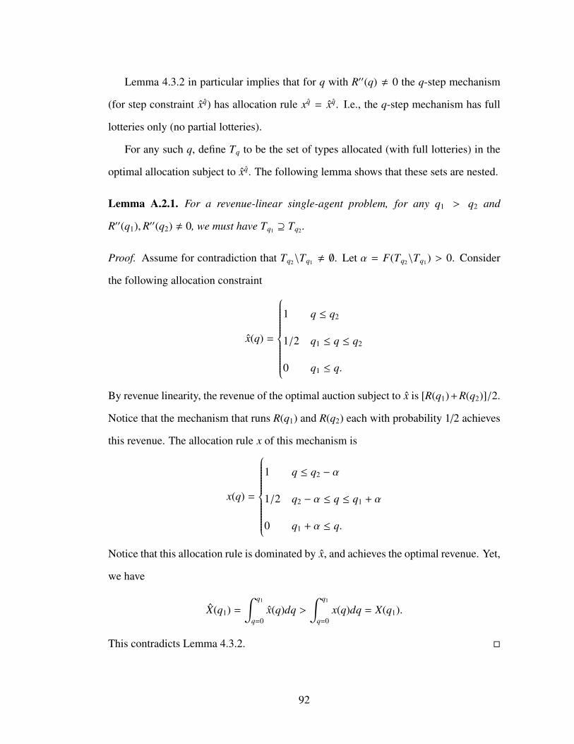
Lemma 4.3.2 in particular implies that for q with R′′(q) , 0 the q-step mechanism

(for step constraint xq) has allocation rule xq = xq. I.e., the q-step mechanism has full

lotteries only (no partial lotteries).

For any such q, define Tq to be the set of types allocated (with full lotteries) in the

optimal allocation subject to xq. The following lemma shows that these sets are nested.

Lemma A.2.1. For a revenue-linear single-agent problem, for any q1 > q2 and

R′′(q1),R′′(q2) , 0, we must have Tq1 ⊇ Tq2 .

Proof. Assume for contradiction that Tq2\Tq1 , ∅. Let α = F(Tq2\Tq1) > 0. Consider

the following allocation constraint

x(q) =

1 q ≤ q2

1/2 q1 ≤ q ≤ q2

0 q1 ≤ q.

By revenue linearity, the revenue of the optimal auction subject to x is [R(q1)+R(q2)]/2.

Notice that the mechanism that runs R(q1) and R(q2) each with probability 1/2 achieves

this revenue. The allocation rule x of this mechanism is

x(q) =

1 q ≤ q2 − α

1/2 q2 − α ≤ q ≤ q1 + α

0 q1 + α ≤ q.

Notice that this allocation rule is dominated by x, and achieves the optimal revenue. Yet,

we have

X(q1) =

∫ q1

q=0x(q)dq >

∫ q1

q=0x(q)dq = X(q1).

This contradicts Lemma 4.3.2.

92

A.3 Linearity

In this section we prove the linearity of the unit demand problem when the distribution

of items is U[0, 1]m for any number of items m. We use the following lemma first noted

by Rochet [47].

Lemma A.3.1. Utility function u corresponds to a truthful mechanism if and only if it is

convex. In this case, p(t) = ∇u · t − u(t), and x(t) = ∇u(t).

Therefore, the allocation of a type t is |∇u(t)|, the L1 norm of the vector ∇u(t). Let

W be the space of convex utility functions u. Let c be the cost of producing an item.

Using the above lemma, we can reformulate the rev problem as follows:

maximize∫

T[∇u(t) · t − u(t)] f (t) dt − c~1 ·

∫T∇u(t) f (t) dt

s.t. u ∈ W

∀S ⊆ T,∫

S|∇u(t)| dt ≤ X( f (S )).

For any t ∈ T , define the function rt : [0, 1]→ T as follows:

rt(x) = x · t

Notice that r(0) = 0, and r(1) = t. We now use the gradient theorem and write

∀t, u(t) − u(0) =

∫ 1

0∇u(r(x)) · r′(x) dx.

In the optimal solution, u(0) = 0. Also, by definition of r, r′(x) = t. Therefore we

have

u(t) =

∫ 1

0∇u(x · t) · t dx.

93

Using the above equation, we can rewrite the objective function as∫T∇u(t) · (t − c~1) −

∫ 1

0∇u(x · t) · t dx dt

=

∫T∇u(t) · (t − c~1) dt −

∫ 1

0

∫T∇u(x · t) · t dt dx.

In the second term, change variables by defining v = (v1, v2) = xt. Notice that

t = v/x, and dvi = xdti for any 1 ≤ i ≤ m. Therefore dv = dt/xm. Define Tx to be t ∈ T

such that maxt1,t2 ≤ x. The objective is∫T∇u(t) · (t − c~1) dt −

∫ 1

0

∫v∈Tx

∇u(v) · (v/x) · (1/xm) dv dx

=

∫T∇u(t) · (t − c~1) dt −

∫v∈T∇u(v) · v

∫ 1

x=maxi vi

1/xm+1 dx dv

=

∫T∇u(t) · (t − c~1) dt −

∫v∈T∇u(v) · v(

1m maxm vi

−1m

) dv

=

∫T∇u(t) · [t(1 +

1m−

1m maxm ti

) − c~1] dt

=

∫T∇u(t) · [t(

m + 1m−

1m maxm ti

) − c~1] dt.

We now show that relaxing the convexity constraint on u does not affect the optimum

solution. Consider a type t such that t1 = maxi ti (the other cases are similar). Since

∇1u(t), . . . ,∇mu(t) appear in the same set of constraints, we can assume that ∇iu(t) = 0

for all i , 1 in the optimum solution. We can therefore remove such variables. This

converts the problem into a polymatroid optimization. Since (maxi ti)(m+1m −

1m maxm ti

) is

non-decreasing in t and the the feasibility constraints are symmetric, we conclude that

types are ordered by maxi ti. This implies that the optimum solution is as follows:

u(t) =

0 maxi ti ≤ tc∫ maxi ti

x=tcX′(1 − xm) dx maxi ti > tc,

where tc solves

t(m + 1

m−

1mtm ) = c

94

Note, for example, that t0 =m√

1m+1 . This function u specified above is convex and

linear in X.

A.4 Proofs from Section 4.4.2

We now give a general procedure for implementing marginal revenue maximization with

general agents. Consider an agent with interim allocation constraint xMR (from marginal

revenue maximization) and mix over q-constrained lottery pricing with probability den-

sity given by − ddq xMR(q) to get outcome rule wMR. Recall each ex ante constrained lottery

pricing is derived by optimizing revenue subject to a step function constraint on the al-

location rule. The resulting outcome rule induces a normalized allocation rule that may

not be a step function. Therefore, xMR is dominated by but not necessarily equal to xMR.

A natural approach to deriving an ordering on types and thus mapping types to quan-

tiles would be to use the mapping given by Quant(·) for xMR, where quantile of a type

is the probability that a type drawn at random has a higher probability of service. This

approach would result in allocation rule xMR not the desired allocation rule xMR. Instead

the map from types to quantiles needs to be randomized to make it “worse” and equal

to the desired allocation rule xMR.

For uniform distributions over discrete type spaces, domination of allocation rules

is equivalent to vector majorization. Hardy, Littlewood, and Polya [30] show a trans-

formation can be given between one and the other via a doubly stochastic matrix. This

implies an algorithm for mapping types to quantiles based on solving a quadratic sized

linear program: solve for the doubly stochastic matrix that gives xMR from xMR, map an

agent type to quantile via Quant(·) induced by xMR, and randomly map this quantile to

a distribution over quantiles by sampling according to the probabilities in the quantile’s

row in the matrix.

As we do not need to construct the matrix, but only to sample from a specific row

95

there is a much simpler construction. This construction further generalizes to non-

uniform distributions. Instead of permutation matrices this approach is based on apply-

ing a sequence of interval resamplings. An interval resampling is given by an interval

[a, b] and if the quantile is in [a, b] it is resampled uniformly from [a, b], otherwise it is

unchanged. For allocation rule x, resampling quantiles from [a, b] has the effect of re-

placing the interval of the cumulative allocation rule X with the line segment connecting

(a, X(a)) to (b, X(b)). The construction below, for type spaces of size m = |T |, calculates

the requisite sequence of at most m interval resamplings in linear time.

Definition A.4.1. For allocation constraint x and dominated allocation rule x satisfying

X(1) = X(1) on m discrete types, the interval resampling sequence construction starts

with x(0) = x and calculates x( j+1) from x( j) while x( j) , x as follows.

(a) Find the highest quantile q where x(q) , x( j)(q).

(b) Let q′ > q be the quantile at which the line tangent to X at q with slope x(q) crosses

X( j).2

(c) The jth resampling interval is [q, q′].

(d) Let x( j+1) be x( j) averaged on [q, q′].

Proposition A.4.1. The interval sampling sequence construction gives a sequence of

at most m intervals such that the composition of x with the sequence of resamplings

applied to Quant(·) is equal to x.

Proof. The proof is by induction on j where the jth step assumes the first j− 1 types, in

order of Quant(·), satisfy x( j−1)(Quant(t)) = x(Quant(t)). Consider step j. The assump-

tion that X(1) = X(1) ensures that the intersection of the tangent happens at a q′ ≤ 1.

The line segment connecting interval [q, q′] of X( j) has slope equal to x(q), by definition.2For discrete type, this intersection may happen at a quantile q′ that does not correspond to the bound-

ary between two types. When this happens split the type into two types each occurring with the same totalprobability and with the boundary between them at q′.

96

Therefore, the jth step in the construction leaves x( j)(Quant(t)) = x(Quant(t)) for the

jth type. The procedure is linear time as both x and x are, without loss of generality,

piece-wise constant with m pieces, and in each step q and q′ are increasing and at least

one piece from x or x is processed.

The final ingredient in the construction of the marginal revenue mechanism for

agents with general types is in converting the allocation rule back into an outcome rule.

This can be done exactly as in Alaei et al. [1]: if an agent with type t is served by the

allocation rule, sample from service outcomes of wMR(t), otherwise sample from non-

service outcomes of wMR(t).

Definition A.4.2. The marginal revenue mechanism for general agents works as follows.

(a) Map reported types t = (t1, . . . , tn) of agents to quantiles q = (q1, . . . , qn) by, for

each agent, composing the interval resampling transformation with Quant(·).

(b) Calculate the marginal revenue of each agent i as R′i(qi).

(c) Calculate the set of agents to be served by marginal revenue maximization.

(d) Calculate outcomes for each agent i as:

• sample wi ∼ wMRi (ti) conditioned on Alloc(wi) = 1 if i is to be served, or

• sample wi ∼ wMRi (ti) conditioned on Alloc(wi) = 0 if i is not to be served.

Note that instead of calculating outcome rules by mixing over step mechanisms we

could, from the allocation constraint xMR for an agent, calculate the optimal mechanism

subject to that constraint, i.e., with outcome rule Outcome(xMR) and revenue Rev(xMR).

The construction above can be invoked with this outcome rule in place of wMR without

modification; this change generally improves revenue.

The assumption in the interval resampling sequence construction that the allocation

constraint x and the desired allocation x have cumulative allocations satisfying X(1) =

97

X(1) can be removed in downward closed settings. With this constraint removed the

line tangent to X at q may be strictly below X at 1. If this happens we set q′ = 1 and

probabilistically reject a quantile falling in this interval. The probability of rejection is

set so that the slope of the resampled allocation rule is x(q).

Proposition A.4.2. In downward closed settings, a normalized allocation rule x domi-

nated by an allocation rule x, where X(1) > X(1), can still be implemented by interval

resamplings given in Definition A.4.1, and a marginal revenue mechanism for x can run

similarly as in Definition A.4.2.

We use x x to refer to this weaker definition of dominance in downward closed

settings.

A.5 Proofs for unit-demand approximation

Theorem 4.5.3 is a consequence of the two lemmas below and Proposition 4.5.2.

Lemma A.5.1. Twice the optimal representative revenue is a linear upper bound on the

optimal unit-demand revenue.

Proof. Linearity follows simply from the revenue linearity of single-dimensional agents.

Consider the distribution of the maximum virtual value (or zero if the maximum virtual

value is negative) in the representative environment. Index this distribution by quantile

as ψmax(q). The optimal revenue for any allocation constraint x is Eq[ψmax(q)x(q)] which

is linear in x; this follows from the proof that the optimal revenue in single-dimensional

environments is the virtual surplus maximizer.

We now show that twice the optimal representative revenue upper bounds the opti-

mal unit-demand revenue. To do this we will give two auctions for the representative

environment with the allocation constraint x and show that the sum of these auctions’

98

revenue upper bounds the optimal unit-demand revenue for the same constraint. Of

course, optimal representative revenue upper bounds each of these auctions revenue.

A mechanism for the unit-demand problem is simply a lottery pricing, i.e., it is a

set of lotteries L with each ` ∈ L taking the form of (p`, π`1, . . . , π`m) with

∑j π

`j ≤ 1.

The semantics of a lottery ` is that the agent pays the price p` and then is allocated an

item j at random with probability π`j; the semantics of the collection of lotteries L is that

the agent, upon drawing her type from the distribution, chooses the lottery ` ∈ L that

maximizes her utility (or none).

Given any collection of lotteries L that satisfies the allocation constraint x we define

two auctions for the representative environment that have combined revenue at least that

of the collection of lotteries in the unit-demand environment.

The L mimicking auction considers the profile of values v = (v1, . . . , vm) of the repre-

sentatives and the lottery ` ∈ L that would have been selected by the unit-demand agent

with these values. It serves the representative j with the highest value with probability

π`j and charges her p` −∑

j′, j π`j′v j′ + µ(v(2)) where µ(v(2)) is the expected utility of the

unit-demand agent with valuation profile v(2) which is v with v j replaced with max j′, j v j′ .

Notice that the utility of the winning representative j in this auction is exactly the same

as the unit-demand agent less an amount that is a function only of the values of the other

representatives, v− j. As the utility of the unit-demand agent is monotone in her value

for each item, the utility each representative has for winning is negative when she is not

the highest valued representative and positive when she is. Therefore, this auction is

incentive compatible, has revenue at least p`j −∑

j′, j π`j′v j′ on valuation profile v where

j is the highest valued representative, and satisfies allocation constraint x. For a given

valuation profile, call the second term in the winning agent’s payment the deficit of the

L mimicking auction.

The motivation for the next auction is that we want to obtain back the deficit lost

99

by the L mimicking auction. Notice that the procedure that charges the highest valued

representative the second highest value and serves with probability∑

j π`j satisfies the al-

location constraint x and more than balances the deficit; however, it may not be incentive

compatible.

The allocation constrained second-price auction sells to the highest valued repre-

sentative at the second highest representative’s value so as to maximize revenue subject

to the allocation constraint x that any representative is served. Consider the distribution

of the second order statistic of values and let ν(2)(q) be the value that the q quantile of

this random variable takes on. The optimal revenue obtainable via a second price auc-

tion with allocation constraint x is Eq[ν(2)(q)x(q)]. To obtain this revenue, conditioning

on the second highest value being v, with probability x(ν−1(2)(v)) we serve the highest val-

ued representative and charge her v. This auction is incentive compatible and revenue

optimal (in expectation) among all second-price procedures that meet the allocation con-

straint. Therefore, it more than covers the expected deficit of the L mimicking auction.

We have given two incentive compatible auctions for the representative environ-

ment with combined expected revenue exceeding the revenue of the lottery pricing L.

Therefore, twice the optimal representative revenue is at least the optimal unit-demand

revenue.

Lemma A.5.2. The pseudo revenue curve R(·) from uniform virtual pricings for a unit-

demand agent 2-approximates the optimal representative revenue curve (as a function

of q for any q-step constraint).

Proof. Denote the optimal representative revenue for the q-step constraint as a function

of q by the revenue curve ORR(q). Consider the outcome of the optimal auction for the

representative environment with ex ante service constraint q. It sets a uniform virtual

price (denoted ψ(q)) and serves the agent with the highest virtual value strictly bigger

than ψ(q) with probability one. If the probability that the largest virtual value is equal

100

to ψ(q) is strictly positive (which might happen if any virtual value function is constant

on an interval, e.g., from ironing), it probabilistically accepts or rejects the maximum

virtual value when it is equal to ψ(q) so as to serve with the desired ex ante probability

q. The optimal representative revenue can thus be calculated and bounded as follows.

Let (ψ1, . . . , ψm) denote the profile of virtual values of the representatives.

ORR(q) = q · ψ(q) + E[maxi(ψi − ψ(q))+]

≤ q · ψ(q) +∑

iE

[(ψi − ψ(q))+] .

Above, the notation (ψi − ψ(q))+ is short-hand for max(0, ψi − ψ(q)).

Now we show a lower bound on R(q) for q that does not require probabilistic ac-

ceptance in the optimal representative auction described above; denote by Q ⊂ [0, 1] all

such quantiles. Let Ei denote the event that ψ j < ψ(q) for all j , i; our lower bound on

the pseudo q-constrained lottery pricing revenue will ignore contributions to the virtual

surplus from the case that more than one representative has virtual value at least ψ(q).

R(q) ≥ q · ψ(q) +∑

iE

[(ψi − ψ(q))+ | Ei

]· Pr [Ei]

≥ q · ψ(q) + (1 − q) ·∑

iE

[(ψi − ψ(q))+ | Ei

]= q · ψ(q) + (1 − q) ·

∑iE

[(ψi − ψ(q))+] .

The second inequality followed because Pr[Ei], the probability of the event that ψ j <

ψ(q) for all j , i is not less than the probability that ψ j < ψ(q) for all j, which is (1− q).

To extend this lower bound on R(q) from q ∈ Q to all q ∈ [0, 1], consider inserting a

virtual value ψ′ = ψ(q)+ε with measure zero in the distribution. The q′ that corresponds

to serving this virtual value or higher has revenue bounded by the formula above but

ψ′ ≈ ψ(q). Keeping the virtual value constant and varying q in the formula interpolates

a line between the two revenues. As the pseudo ex ante constrained lottery pricings are

closed under convex combination, this line gives a lower bound on the pseudo q-step

mechanism. Therefore, the bound above on R(q) holds for all q.

101

To bound ORR(q) in terms of R(q) we consider two cases. When q ≤ 1/2 these

terms can be directly bounded as the first terms in both bounds are the same and the

second terms are within a factor of two of each other (by assumption 1 − q ≥ 1/2).

When q ≥ 1/2 we can compare the bound on ORR(q = 1) to the bound on R(q = 1/2);

these bounds are within a factor of two of each other. Monotonicity (via downward

closure) of ORR(q) and R(q) then implies that they are within a factor of two for any

q ∈ [1/2, 1].

102

BIBLIOGRAPHY

[1] Saeed Alaei, Hu Fu, Nima Haghpanah, Jason Hartline, and Azarakhsh Malekian.

Bayesian optimal auctions via multi- to single-agent reduction. In ACM Confer-

ence on Electronic Commerce, 2012.

[2] Saeed Alaei, Hu Fu, Nima Haghpanah, and Jason Hartline. The simple economics

of approximately optimal mechanisms. In FOCS, 2013.

[3] Noga Alon, Yuval Emek, Michal Feldman, and Moshe Tennenholtz. Bayesian

ignorance. In PODC, pages 384–391, 2010.

[4] Pablo Azar, Constantinos Daskalakis, Silvio Micali, and Matthew Weinberg. Op-

timal and efficient parametric auctions. In SODA, 2013.

[5] Kshipra Bhawalkar and Tim Roughgarden. Welfare guarantees for combinatorial

auctions with item bidding. In SODA, pages 700–709, 2011.

[6] Kshipra Bhawalkar and Tim Roughgarden. Simultaneous single-item auctions. In

WINE, 2012.

[7] Sushil Bikhchandani. Auctions of heterogeneous objects. Games and Economic

Behavior, 26(2):193–220, January 1999.

[8] Patrick Briest, Shuchi Chawla, Robert Kleinberg, and S. Matthew Weinberg. Pric-

ing randomized allocations. In ACM-SIAM Symposium on Discrete Algorithms,

pages 585–597, 2010.

[9] Jeremy Bulow and John Roberts. The simple economics of optimal auctions. Jour-

nal of Political Economy, 97(5):1060–90, October 1989.

[10] Yang Cai and Constantinos Daskalakis. Extreme-value theorems for optimal mul-

tidimensional pricing. Foundations of Computer Science, 2011.

103

[11] Yang Cai, Constantinos Daskalakis, and S. Matthew Weinberg. An algorithmic

characterization of multi-dimensional mechanisms. In STOC, pages 459–478,

2012.

[12] Yang Cai, Constantinos Daskalakis, and S. Matthew Weinberg. Optimal multi-

dimensional mechanism design: Reducing revenue to welfare maximization. In

FOCS, 2012.

[13] Yang Cai, Constantinos Daskalakis, and Matthew Weinberg. Reducing revenue

to welfare maximization: Approximation algorithms and other generalizations. In

SODA, 2013.

[14] Ioannis Caragiannis, Panagiotis Kanellopoulos, Christos Kaklamanis, and Maria

Kyropoulou. On the efficiency of equilibria in generalized second price auctions.

In EC, pages 81–90, 2011.

[15] S. Chawla, D. Malec, and B. Sivan. The power of randomness in bayesian optimal

mechanism design. In EC, pages 149–158, 2010.

[16] Shuchi Chawla, Jason D. Hartline, David L. Malec, and Balasubramanian Sivan.

Multi-parameter mechanism design and sequential posted pricing. In STOC, pages

311–320, 2010.

[17] George Christodoulou, Annamaria Kovacs, and Michael Schapira. Bayesian com-

binatorial auctions. In ICALP (1), pages 820–832, 2008.

[18] E. H. Clarke. Multipart pricing of public goods. Public Choice, pages 17–33,

1971.

[19] Jacques Cremer and Richard P McLean. Optimal selling strategies under uncer-

tainty for a discriminating monopolist when demands are interdependent. Econo-

metrica, 53(2):345–61, March 1985.

104

[20] Constantinos Daskalakis, Alan Deckelbaum, and Christos Tzamos. The complex-

ity of optimal mechanism design. 2012. manuscript.

[21] Peerapong Dhangwatnotai, Tim Roughgarden, and Qiqi Yan. Revenue maximiza-

tion with a single sample. In ACM Conference on Electronic Commerce, pages

129–138, 2010.

[22] Shahar Dobzinski, Hu Fu, and Robert D. Kleinberg. Optimal auctions with corre-

lated bidders are easy. In STOC, pages 129–138, 2011.

[23] Benjamin Edelman, Michael Ostrovsky, Michael Schwarz, Thank Drew Fuden-

berg, Louis Kaplow, Robin Lee, Paul Milgrom, Muriel Niederle, and Ariel Pakes.

Internet advertising and the generalized second price auction: Selling billions of

dollars worth of keywords. American Economic Review, 97, 2005.

[24] Uriel Feige. On maximizing welfare when utility functions are subadditive. SIAM

J. Comput., 39(1):122–142, 2009.

[25] Michal Feldman, Hu Fu, Nick Gravin, and Brendan Lucier. Simultaneous auctions

are (almost) efficient. In STOC, pages 201–210, 2013.

[26] Hu Fu. Vcg auctions with reserve prices: Lazy or eager? 2013. In submission.

[27] Hu Fu, Robert Kleinberg, and Ron Lavi. Conditional equilibrium outcomes via

ascending price processes with applications to combinatorial auctions with item

bidding. In ACM Conference on Electronic Commerce, page 586, 2012.

[28] T. Groves. Incentives in teams. Econometrica, pages 617–631, 1973.

[29] Faruk Gul and Ennio Stacchetti. Walrasian equilibrium with gross substitutes.

Journal of Economic Theory, 87(1):95–124, July 1999.

105

[30] G. Hardy, J. Littlewood, and G. Polya. Some simple inequalities satisfied by con-

vex functions. Messenger of Math, 58:145–152, 1929.

[31] Jason D. Hartline and Brendan Lucier. Bayesian algorithmic mechanism design.

In STOC, pages 301–310, 2010.

[32] Jason D. Hartline and Tim Roughgarden. Simple versus optimal mechanisms. In

ACM Conference on Electronic Commerce, pages 225–234, 2009.

[33] Jason D. Hartline, Robert Kleinberg, and Azarakhsh Malekian. Bayesian incentive

compatibility and matchings. In SODA, 2011.

[34] Avinatan Hassidim, Haim Kaplan, Yishay Mansour, and Noam Nisan. Non-price

equilibria in markets of discrete goods. In ACM Conference on Electronic Com-

merce, pages 295–296, 2011.

[35] Elias Koutsoupias and Christos Papadimitriou. Worst-case equilibria. In STACS,

pages 404–413, 1999.

[36] Benny Lehmann, Daniel J. Lehmann, and Noam Nisan. Combinatorial auctions

with decreasing marginal utilities. Games and Economic Behavior, 55(2):270–

296, 2006.

[37] Renato Paes Leme and Eva Tardos. Pure and bayes-nash price of anarchy for

generalized second price auction. In FOCS, pages 735–744, 2010.

[38] Brendan Lucier and Allan Borodin. Price of anarchy for greedy auctions. In SODA,

pages 537–553, 2010.

[39] Brendan Lucier and Renato Paes Leme. Gsp auctions with correlated types. In

EC, pages 71–80, 2011.

[40] S. Mamer, J.and Bikhchandani. Journal of Economic Theory, 74:385–413, 1997.

106

[41] Evangelos Markakis and Orestis Telelis. Uniform price auctions: Equilibria and

efficiency. In SAGT, pages 227–238, 2012.

[42] Paul Milgrom. Putting auction theory to work: The simultaneous ascending auc-

tion. Journal of Political Economy, 108:245–272, 1998.

[43] Roger B. Myerson. Optimal auction design. Mathematics of Operations Research,

6(1):pp. 58–73, 1981. ISSN 0364765X.

[44] Noam Nisan, Tim Roughgarden, Eva Tardos, and Vijay V. Vazirani. Algorithmic

Game Theory. Cambridge University Press, New York, NY, USA, 2007. ISBN

0521872820.

[45] Christos Papadimitiou and George Pierrakos. On optimal single-item auctions. In

STOC, pages 119–128, 2011.

[46] David Rahman. Surplus extraction on arbitrary type spaces. Theoretical Eco-

nomics, 2012.

[47] J.C. Rochet. The taxation principle and multi-time hamilton-jacobi equations.

Journal of Mathematical Economics, 14(2):113 – 128, 1985. ISSN 0304-4068.

[48] Amir Ronen. On approximating optimal auctions. In ACM Conference on Elec-

tronic Commerce, pages 11–17, 2001.

[49] Tim Roughgarden and Eva Tardos. Introduction to the inefficiency of equilibria.

In Noam Nisan, Tim Roughgarden, Eva Tardos, and Vijay V. Vazirani, editors,

Algorithmic Game Theory. Cambridge University Press, New York, NY, USA,

2007.

[50] Alexander Schrijver. Combinatorial Optimization : Polyhedra and Efficiency (Al-

gorithms and Combinatorics). Springer, July 2003. ISBN 3540204563.

107

[51] Vasilis Syrgkanis. Bayesian games and the smoothness framework. CoRR,

abs/1203.5155, 2012.

[52] John Thanassoulis. Haggling over substitutes. J. Economic Theory, 117(2):217–

245, 2004.

[53] Hal R. Varian. Position auctions. International Journal of Industrial Organization,

25(6):1163–1178, December 2007.

[54] W. Vickrey. Counterspeculation, auctions and competitive sealed tenders. Journal

of Finance, pages 8–37, 1961.

[55] Robert Wilson. Nonlinear Pricing. Oxford University Press, 1997.

[56] Qiqi Yan. Mechanism design via correlation gap. In SODA, 2011.

108