Similarity-based Classifier Combination for Decision Making

Authors: Gongde Guo, Daniel Neagu

Department of Computing, University of Bradford

Outline of PresentationOutline of Presentation

1.1. BackgroundBackground– Classification process;– Drawbacks of A Single Classifier– Solutions …

2.2. Approaches for Multiple Classifier SystemsApproaches for Multiple Classifier Systems– Explanation of the Four Approaches

3.3. An Architecture of Multiple Classifier SystemAn Architecture of Multiple Classifier System4.4. Involved Classifiers for CombinationInvolved Classifiers for Combination

– K-Nearest Neighbour Method (kNN)– Weighted k-Nearest Neighbour Method (wkNN)– Contextual Probability-based Classification (CPC)– kNN Model-based Method (kNNModel)

5.5. Combination StrategiesCombination Strategies– Majority voting –based combination– Maximal Similarity-based Combination– Average Similarity-based Combination– Weighted Similarity-based Combination

6.6. Experimental ResultsExperimental Results7.7. ConclusionsConclusions8.8. ReferenceReference

Background - Background - Classification ProcessClassification Process Classification occurs in a wide range of human activities. At

its broadest, the term could cover any activity in which some decision or forecast is made on the basis of currently available information, and a classifier is then some formal method for repeatedly making such judgments in new situations (Michie et al. 1994) .

Various approaches to classification have been developed and applied to real-world applications for decision making. Examples include probabilistic decision theory, discriminant analysis, fuzzy-neural networks, belief networks, non-parametric methods, tree-structured classifiers, and rough sets.

Background - Background - Drawbacks of A Single ClassifierDrawbacks of A Single Classifier

Unfortunately, no dominant classifier exists for all the data

distributions, and the data distribution of the task at hand is usually unknown. A single classifier cannot be discriminative enough if the number of classes is huge. For applications where the classes of content are numerous, unlimited, and unpredictable, one specific classifier cannot solve the problem with a good accuracy.

Background - Background - SolutionsSolutions

A Multiple Classifier System (MCS) is a powerful solution to difficult decision making problems involving large sets and noisy input because it allows simultaneous use of arbitrary feature descriptors and classification procedures.

The ultimate goal of designing such a multiple classifier system is to achieve the best possible classification performance for the task at hand. Empirical studies have observed that different classifier designs potentially offer complementary information about the patterns to be classified, which could be harnessed to improve the performance of the selected classifier.

Architecture of Multiple Classification SystemsArchitecture of Multiple Classification Systems

Approach 1: Different combination schemes. Approach 2: Different classifier models.

Classifier iClassifier 1 Classifier L

Combiner

x

Classifier iClassifier 1 Classifier L

Combiner

x

……

Combiner

x

Approach 3: Different feature subsets.

…

D1 Di Dm

Approach 4: Different training sets.

…

S1 SkSi

Classifier iClassifier 1 Classifier L

n n

Given a set of classifiers C={C1, C2, …, CL} and a dataset D, each instance x in D represents as a

feature vector [x1, x2, …, xn]T, x

A classifier gets as its input x and assigns it to a class label from Ω, i.e.

Four approaches are generally used to design a classifier combination system (Kuncheva, 2003).

Explanation of the Four ApproachesExplanation of the Four Approaches

Approach 1:Approach 1: The problem is to pick a combination scheme for The problem is to pick a combination scheme for LL classifiers classifiers CC11, , CC22, …, , …, CCLL studied to form a combiner. studied to form a combiner.

Approach 2:Approach 2: The problem is to choose individuals (classifiers) The problem is to choose individuals (classifiers) by considering the issues of similarity/ diversity, by considering the issues of similarity/ diversity, homogeneous/heterogeneous etc. homogeneous/heterogeneous etc.

Approach 3:Approach 3: The problem is to build each The problem is to build each CCii on an individual on an individual

subset of features (subspace of )subset of features (subspace of )Approach 4:Approach 4: The problem is to select training subsets The problem is to select training subsets DD11,, D D22, ,

…, …, DDmm of the dataset of the dataset DD to lead to a team of diverse classifiers. to lead to a team of diverse classifiers.

n

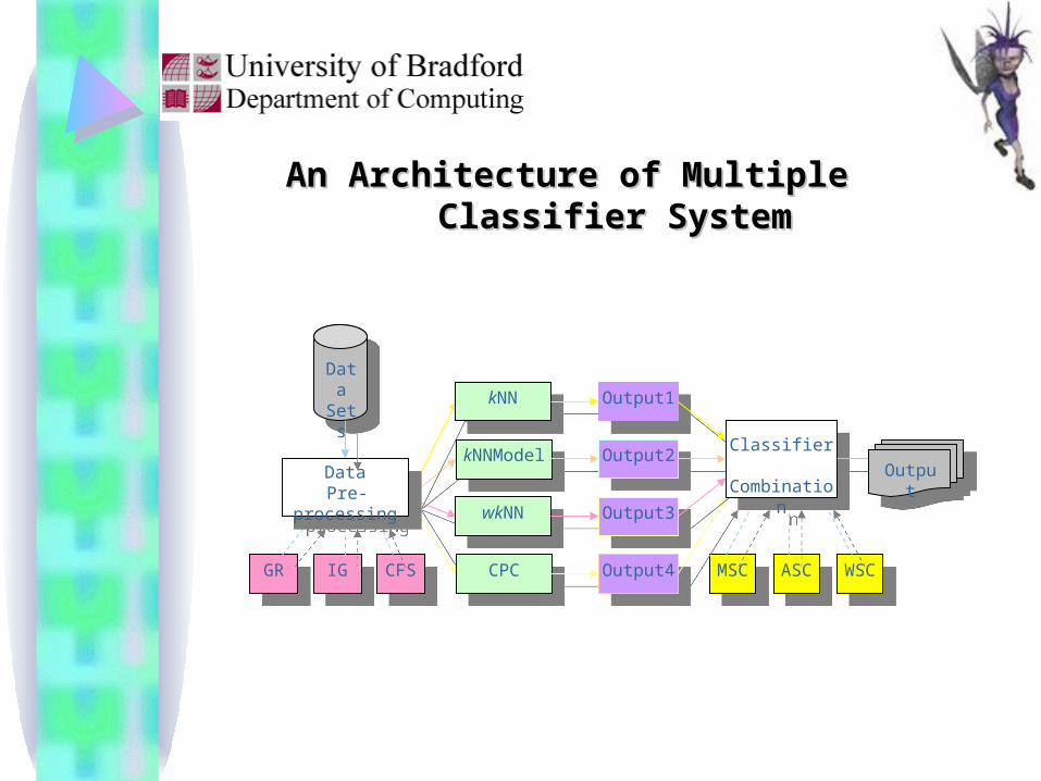
An Architecture of Multiple Classifier SystemAn Architecture of Multiple Classifier System

GRGR

IGIG

CFSCFS

MSCMSC

ASCASC

WSCWSC

CPCCPC

wkNNwkNN

kNNModelkNNModel

kNNkNN

Output4Output4

Output3Output3

Output2Output2

Output1Output1

Classifier Combination

Classifier Combination Output

Data Pre-processing

Data Pre-processing

DataSets

Involved Classifiers for Combination- Involved Classifiers for Combination- kkNNNN

Given an instance x, the k-nearest neighbour classifier finds its k nearest instances, and traditionally uses the majority rule (or majority voting rule) to determine its class, i.e. assigning the single most frequent class label associated with the k nearest neighbours to x. This is illustrated in Figure 3. The two classes here are depicted by “□” and “o”, with ten instances for each class. Each instance is represented by a two-dimensional point within a continuous-valued Euclidean space. The instance x, represented as ‘ ’.

x

k=5

In wkNN, the k nearest neighbours are assigned different weights. Let ∆ be a distance measure, and x1, x2, …, xk be the k nearest

neighbours of x arranged in increasing order of ∆(xi, x). So x1 is the

first nearest neighbour of x. The distance weight wi for i-th neighbour

xi is defined as follows:

),(),(

),(),(

1),(),(

),(),(

1

1

1 xxxxif

xxxxifxxxx

xxxxw

k

k

k

ik

i

Instance x is assigned to the class for which the weights of the representatives among the k nearest neighbours sum to the greatest value.

Involved Classifiers for Combination-Involved Classifiers for Combination- wkwkNNNN

Contextual probability-based classifier (CPC) (Guo et al., 2004) is based on a new function G – a probability function used to calculate the support of overlapping or non-overlapping neighbourhoods. The idea of CPC is to aggregate the support of multiple sets of nearest neighbours of a new instance for various classes to give a more reliable support value, which better reveals the true class of this instance.

Involved Classifiers for Combination- Involved Classifiers for Combination- CPCCPC

Involved Classifiers for Combination- Involved Classifiers for Combination- kkNNModelNNModel

The basic idea of kNN model-based classification method (kNNModel) (Guo et al. 2003) is to find a set of more meaningful representatives of the complete data set to serve as the basis for further classification. Each chosen representative xi is represented in the form of <Cls(xi), Sim(xi), Num(xi), Rep(xi)> which respectively represents the class label of xi; the similarity of xi to the furthest instance among the instances covered by Ni; the number of instances covered by Ni; a representation of intance xi. The symbol Ni represents the area that the distance to Ni is less than or equal to Sim(xi). kNNModel can generate a set of optimal representatives via inductively learning from the dataset.

Combination StrategyCombination Strategy––Majority Voting-based CombinationMajority Voting-based Combination

},,...,,{ 21 mcccC

iAf Cn

k

iACc xfc

i

1

))(,(maxarg

1),( ba 0),( ba

Given a new instance x to be classified, whose true class label is tx and k predefined classifiers are denoted as A1, A2,

…, Ak respectively, the classifier Ai approximates a discrete-valued function

:The final class label of x, obtained by using majority voting-based classifier combination, is described as follows:

f(x)

where if a=b, and otherwise

Combination StrategyCombination Strategy

– – Class-wise similarity-based classifier combinationClass-wise similarity-based classifier combination

},...,1|},...,1{max{maxarg)(1 mvkuSxf uvCcv

k

uuvCc mvkSxf

v

12 },...,2,1|)/({maxarg)(

},...,2,1|max{{{maxarg)( ,3 kuSxf uvCcv

},...,2,1|)}/()1(1

mvkSk

uuv

10

The classification result of x classified by Aj is given by a vector of normalized

similarity values of x to each class, represented by S = <Sj1, Sj2, …, Sjm>, where

j=1, 2, …, k. The final class label of x can be obtained in three different ways:a) Maximal Similarity-based Combination (MSC):

b) Average Similarity-based Combination (ASC):

c) Weighted Similarity-based Combination (WSC):

, where is a control parameter used for setting the relative importance of

local optimization and global optimization of combination.

This study mainly focuses on Approach 1. Given four classifiers: kNN, kNNModel, CPC and wkNN, we proposed three similarity-based classifier combination schemes empirically. After evaluating them on fifteen public datasets from UCI machine learning repository, we apply the best approach to a real-world application of toxicity prediction of the environment effects of chemicals in order to obtain better classification performance.

Experimental ResultsExperimental Results

In Table 1, NF-Number of Features, NN-Number of Nominal features, NO-Number of Ordinal features, NB-Number of Binary features, NI-Number of Instances, CD-Class Distribution. Four Phenols data sets are used in the experiment, where Phenols_M represents the phenols data set with MOA (Mechanism of Action) as endpoint for prediction; Phenols_M_FS represents the Phenols_M data set after feature selection; Phenols_T represents the Phenols data set with toxicity as endpoint for prediction, and Phenols_T_FS represents Phenols_T data set after feature selection.

Fifteen public data sets from the UCI machine learning repository and one data set (Phenols) from real-world applications (toxicity prediction of chemical compounds) have been collected for training and testing. Some information about these data sets is given in Table 1.

Data set NF NN NO NB NI CD

AustralianColicDiabetesGlassHClevelandHeartHepatitisIonosphereIrisLiverBupaSonarVehicle VoteWineZooP_MOAP_MOA_FSP_TP_T_FS

1423

89

13131934

46

6018161316

17320

17320

416

003360000000

160000

6789771

3446

6018

013

0173

20173

20

400033

1200000

16000000

690368768214303270155351150345208846435178

90250250250250

383:307232:136268:500

70:17:76:0:13:9:29164:139120:150

32:123126:225

50:50:50145:200

97:111212:217:218:199

267:16859:71:48

37:18:3:12:4:7:9173:27:4:19:27173:27:4:19:27

37:152:6137:152:61

Table 1. Some information about the data sets

Table 2. A comparison of four individual algorithms and MV in classification performance.

Data set kNNModel ε N vkNN wkNN CPC MV

AustralianColicDiabetesGlassHClevelandHeartHepatitisIonosphereIrisLiverBupaSonarVehicleVoteWineZooP_MOAP_MOA_FSP_TP_T_FS

86.0983.6175.7869.5282.6781.8589.3394.2996.0068.5384.0066.5591.7495.2992.2283.2089.2071.6075.60

211301100202400002 2

5453132122335120044

85.2283.0674.2167.6281.0080.3783.3384.0096.6766.4785.0069.2992.1794.7195.5687.2088.8074.4073.60

82.4681.9472.3767.4281.3377.4183.3387.1495.3366.4786.5071.4390.8795.2995.5686.8092.8074.4072.40

84.6483.6172.6368.5782.6781.4882.6784.8696.0065.8887.5070.1291.7495.8896.6787.6091.2074.8077.20

85.6583.3374.8769.5283.0081.8585.3388.5796.0068.8287.0071.4391.7495.2995.5687.6091.6074.0076.00

Average 83.00 / / 82.25 82.17 82.93 83.53

Table 3. A comparison of different combination schemes

Data set SVM C5.0 MV MSC ASC WSC α ε N

AustralianColicDiabetesGlassHClevelandHeartHepatitisIonosphereIrisLiverBupaSonarVehicleVoteWineZooP_MOAP_MOA_FSP_TP_T_FS

81.4583.8977.1162.8683.6784.0782.6787.1498.6769.7174.0077.5096.9695.2997.7984.4089.2065.6076.00

85.580.976.666.374.975.680.784.592.065.869.467.996.192.191.190.089.272.874.0

85.6583.3374.8769.5283.0081.8585.3388.5796.0068.8287.0071.4391.7495.2995.5687.6091.6074.0076.00

86.5284.7275.1370.9582.3381.8587.3389.4396.6770.5988.5070.8392.6196.4795.5688.4092.4076.4077.20

86.2384.1775.1370.9582.3381.4886.6788.8696.6771.1888.5071.9092.6196.4796.6788.2092.4076.0076.40

86.5284.7275.1370.9582.6781.8587.3389.4396.6771.1889.0071.9092.6196.4796.6788.8092.4076.4077.20

0.70.70.70.70.70.70.60.70.70.80.70.80.70.70.70.80.70.70.7

2342421113222100423

5000045045050000000

Average 82.53 80.28 83.53 84.42 84.39 84.64 / / /

SVM C5.0 kNNModel vkNN wkNN CPC MV

MV -0.69(-)

2.98(+)

-0.33(-)

2.52(+)

2.07(+)

0.23(-)

/

WSC 1.15(-)

2.98(+)

2.07(+)

3.44(+)

2.98(+)

2.98(+)

2.52(+)

Table 4. The signed test of different classifiers

In Table 4, the item 2.07 (+) in cell (3, 4), for example, means WSC is better than kNNModel in terms of performance over the nineteen data sets. That is, the corresponding |Z|>Z0.95=1.729. The item 1.15 (-) in cell (3, 2) means there is no significant difference in terms of performance between WSC and SVM over nineteen data sets as the corresponding |Z|<Z0.95=1.729.

Conclusions

• The proposed methods directly employ class-wise similarity measure used in each individual classifier for combination without changing the representation from similarity to probability. • It significantly improves the average classification accuracy carried out over nineteen data sets. The average classification accuracy of WSC is better than that of any other individual classifiers and the majority voting-based combination method. • The statistical test also shows that the proposed combination method WSC is better than any individual classifier with an exception of SVM.• The average classification accuracy of WSC is still better than that of SVM with a 2.49% improvement. • Further research is required into how to combine heterogeneous classifiers using class-wise similarity-based combination methods.

References

(Michie et al. 1994) D. Michie, D.J.Spiegelhalter, and C.C.Taylor. Machine Learning,

Neural and Statistical Classification, Ellis Horwood, 1994.(Guo et al. 2003) G. Guo, H. Wang, D. Bell, Y. Bi, K. Greer. kNN Model-Based

Approach in Classification. In Proc. of ODBASE 2003, LNCS 2888/2003, pp. 986-996, 2003.

(Guo et al. 2004) G. Guo, H. Wang, D. Bell, Z. Liao. Contextual Probability-Based

Classification. In Proc. of ER 2004, LNCS 3288/2004, pp. 313-326, Springer-Verlag, 2004.

(Kuncheva, 2003) Kuncheva. L.I. Combining Classifiers: Soft Computing

Solutions. In: S.K. Pal (Eds.) Pattern Recognition: From Classical to Modern Approaches, pp. 427-452, World Scientific, Singapore, 2003.

Thank you very much!Thank you very much!