signal theoretic characterization of a function using
TRANSCRIPT
Scholars' Mine Scholars' Mine
Doctoral Dissertations Student Theses and Dissertations
1968
Signal theoretic characterization of a function using positive Signal theoretic characterization of a function using positive
exponential basis functions exponential basis functions
James Julius Baremore
Follow this and additional works at: https://scholarsmine.mst.edu/doctoral_dissertations
Part of the Electrical and Computer Engineering Commons
Department: Electrical and Computer Engineering Department: Electrical and Computer Engineering
Recommended Citation Recommended Citation Baremore, James Julius, "Signal theoretic characterization of a function using positive exponential basis functions" (1968). Doctoral Dissertations. 1917. https://scholarsmine.mst.edu/doctoral_dissertations/1917
This thesis is brought to you by Scholars' Mine, a service of the Missouri S&T Library and Learning Resources. This work is protected by U. S. Copyright Law. Unauthorized use including reproduction for redistribution requires the permission of the copyright holder. For more information, please contact [email protected].

SIGNAL T'HEORE'i'IC G!.LI\l~/\.CTEH IZATION
OF A FUNC:riON USI0~G POSITIVE
EXPOr~EHTIAI, BASIS FUNC'l'IONS
by
19. I•
JULilTS ~A~J~¥~DE ~~ - I .iJ.t:..i\. --·1 ~UJ.\. -;.t
A DISSERTATION
Pr-escnt(;'cl to the Faculty of the Grc:.::duat.e ScLool of the
'lTNIVERSI'.CY OF HISSOU;<I P.'.l' ROl.LA
In Partial Fulfillment of th€ Eequircir]Gnts for the D:::·.sr-:-:2
Advisor
/---» ("..,
C. 7 /~ ~~; - (~- . Lfn.(-~
DOCTOR OF FHIL030.PHY
in
ELECTRICAL EriGJ.NEEH.E'lG ~T.' l \ --1" \ 1--
196j
/ i
. () ,,1
c. \ I p \ ) ... I I
/7 -- - L': . - ,.. -J I" :1 . . I f.. \/ ~-- ' -~ i •. >- . ·. . . - . ) I -' '/ • ' ·-----·- _____ '_/__" ··--···---;-.f:_.~./--,..:.-J.. •. .f_~-~: __ ,--
I
----- ------· .. ····- .~-~- .. ---·--· ·-·-----·--

ii
ABSTRAC'f
A signal theory characterization of a time function or
signal is a representation of the function throughout a
sample interval by an orthogonal basis function expansion.
The characterization described here obtains the coefficie
nts in the expansion by processing the input waveform, in
real time, through a system of three terminal passive RC
filters. The outputs of the filters are sampled periodi
cally and the coefficients of the basis function expansion
in that interval are related to these values. The basis
functions result from an exponential transfo~nation applied
to the Legendre polynomials and are o~·thogonal in time over
the sample interval. The basis functions and the resulting
reconstruction appear as sunnnations· of positive exponential
te:cms.
Different signals may require different sampling
intervals and/or different number of terms in their
orthogonal expansions. As a result_, the input -.;·Javeforms
have been classified in the time dom2.in by two methods.
One is a graphical method. The worst case input to the
system is bounded by simple test functions. The shortest
du·.cation of the resulting test functions gives the sa:nple
interval. The rate of convergence of the mean-square
error of the approximation is also given for the various
forms of the test function.
The graphical technique is easy to us2: but gives
conservative error estimates.
iii
The input waveform is also classified i.n terms of
the pole locations of the Laplace-transfonned input
function. Using conventional time domain synthesis
techniques, the pole locations of the transfo;:med input
function can be located in the complex-S plane. Bounding
these poles by circles, with center at the origin of
the S plane_, will give the maximUt-rl signal reconstru.ction
error for a given number of filt~.:--·rs. The sarepling period
is based on a normalized rate and the frequency scaling
required to move the poles into desirable maximum error
regions of the S plane d~termines the actual smnpling
rate. These reg::_ons are very broad and thus a considerable
change in the pole positions can be tolerated without
affecting the parameters of the system. This method is
more ali.alyt:ical than the first method, although more
work is required to find the pole lee ations.

iv
ACKNOWLEDGEHENTS
The author wishes to express his thanks to Dr. Herbert
M. Barnard and acknowledge the work which was performed
jointly with him during the initial study at Sandia
Corporation.
Thanks are also due to Dr. Edward C. Bertnolli for
his help and guidance in continuing this work.
The author also wishes to express his gratitude-: to
his wife Donna for her consideraticm a:nd understanding
during these five years of graduate work.

TABLE OF CONTENTS
ABSTRACT
ACKNOWLEDGE~lliWfS
LIST OF FIGURES
LIST OF TABLES
I.
II.
III.
IV.
v.
INTRODUCTION
BASIC SIGNAL THEORY SYSTEM
A.
B.
c.
Basis Functions
Filter Realizations 1. Parallel Realizations 2. Input-Output Realizations
Meltiple Sampling
DERIVATIVE APPROXIHATION OF THE SIGNAL
A. Derivation of Results
B. Filter Realizations
DETERHINATION OF ALPHA
GR.i\PHICAL CU~SSIFICATION OF INPUT SIGNAL
A. Polynomial Approximation
First Test Function
c. Second Test Function
v
ii
iv
vii
ix
10
22
25
28 28 36
39
49
54
54
55
66

VI.
VIla
CLASSIFICATION OF INPUT SIGNAL BY POLE LOCATION
A.
B.
Error Analysis
Determination of Pole Locations 1. Time-domain Synthesis 2. Polynomial Approximation
of Input
PROBLEMS FOR FURTHER STUDY
Graphical Test Function
Derivative Approximation
Error Analysis
Bandlimited Signals
BIBLIOGRAPHY
VITA
vi
73
73
83 83
93
105
105
109
111
115
118
121

Figure
1.1
1.2
1.3
2.1
2.2
2.3
2. ~-
2.5
2.6
2.7
3.1
3.2
3.3
4.1
4.2
5.1
5.2
5.3
LIST OF FIGURES
Orthonormal Filter Scheme
Typical Signal to be Represented
Variation of Error with Alpha
Block Diagram of Signal Theory System
Elements of a Composite Filter
Parallel Realization of composite Filters
Reconstruction of F(t)
Reconstruction of F(t) = e -t
Relationship Between A and I n n Input-Output Block Diagram
Two Realizations of D0 (S)
Realization of D2 (s)
Alternate Realization of n2 (s)
Relationship Between x and t as a Function of Alpha
Error Vs. N and Alpha
C (max) Vs. N for First Test Function n
C (max) Vs. N for Second Test Function n
}1SE/F2 Vs. N
vii
Page
17
20
21
24
26
30
31
35
3r{
38
46
47
48
50
52
59
69
70
Figure
7-2
7-3
Pole Location Vs. N for "1 = • 01
Pole Location Vs. N for TJ = • 05
Normal Equations in the Gross Method
Roots of Equation 6.21~ Fourth Order Approximation
Roots of Equation 6.21, Third Order Approximation
Reconstruction Showing the AcCUl.l1ulation of Error
Plot of Error at Sample Points of Fig. 7.1
Reconstruction with Zero Error at the Sample Points
Straight Line Approximation of Input Signal
viii
Page
78
79
89
lOG
103
110
112
113

Table
I.
IIo
III.
IV.
v. VI.
VII.
LIST OF TABLES
Maximum and Minimum Values of C Vso N n
Mean Square Error Vso N
Ratio of NSE to MSV Vs. N
Maximum Values of Cn Vs. N
Pole Locations from Yengst Method
Coefficients of pj(s~2L)
o-2and bj Vs. j
ix
Page
58
61
64
68
86
96
98
CHAPTER I
INTRODUCTION
10
There are many methods of representing a time varying
signal. The Fourier ~eries and ~ower ~eries expansions of
a function are among those most familar to engineers. These
methods have as a basic objective the representation of
a signal by the specification of only a few tabulated
values~ namely the coefficients of the expansiono The
coefficients are determined by evaluating integrals. This
requires a knowledge of the input function throughout the
reconstruction interval. These representations are
usually used in the solution of engineering problems.
Another type of representation) which is used to
describe a waveform which is occuring in real timeJ is
based on the sampling theorem. This theorem states that
if a time function~ f ( t), contains no frequency components
higher than v,~ hertz_, then the time function can be comple
tely determined by specifying its ordinB.tes at a sequence
of times spaced every 1/2\v seconds or less. A waveform
which is not bandlirnited to some upper frequency W can
be filtered by a sharp cutoff low pass filter and the
output of this filter assumed to be a bandlimited signal.
This filtered signal can then be reconstructed from a
knowledge of the sample values. There are several reascms
for prefiltering the signal. One is that the engineer
can decide that the information contained in the frequencys

11
above the cutoff frequency of the prefilter is of no
significance. This allows a slower sampling of the
signal than would be otherwise required. Another reason
is due to hardware limitations which limit the maximum
physical rate at which the signal can be sampled. It is
as a result of this second limitation that the system
described in this work was originally considered. The
signal theory system obtains the information necessary
to represent the waveform by a parallel sampling at a
rate lower than that required for a pure sampling type
system. The input signal, which is to be represented)
is processed simultaneously thru a set of RC filters. The
output of these filters at the end of a predetermined
interval is sufficient to allow the reconstruction of
the signal over that interval. This allows a reduction
in sampling rate, although the &imultaneous sampling may
require more total data points to represent the signa]
than a sampled-data system.
A third type of signal representation, upon which
the signal theory system is a modification, is the
orthonorrn2.l basis function expansion of the signal. This
type of representation has received considerable attention
at John Hopkir.1s University1 . This work shmvs that a signal
may be represented in ten1s of a set of basis functions,

12
as
00
( 1. 1)
The orthonormality of the basis functions over the interval
(oJoo) is defined as
00
0J 0'k ( t ) ~ j ( t ) d t
k/j
k=j
Multiplying both sides of equation 1.1 by 0. (t) and J
integrating over the interv2l gives 00 00
(1. 2)
jF(t) 0'.(t) dt 0 J
= I Ak . f 0k ( t ) 0' . ( t ) d t . ( 1 . 3 ) k=l 0 J
Due to the orthogonality of the basis functions) all terms
on the right hand side of equation 1.3 vanish except the
term for j = k . Therefore the coefficients in the
expansion given by equation 1.1 may be evaluated by the
following integral.
( 1. 4)
Equation 1.1 suggests that an infinite numbe1.· of terms
are needed to represent the function by a basis function
expansion) ho~vever equation 1.1 can be rew·ritten as
N F(t) =}:A 0 (t)
n=ln n
00
+ }:A 0 (t) n n n=N+l
In this expression) the first N tenus will represent the
approximation and the remainder of ·the terms will represent
the error resulting from the use of this approximation.

13
For a given value of N, it is desired to choose the
coefficients so that the mean square error of the N term
approximation is minimized. It can be shov1n2 that the
coefficients given by equation 4 are sufficient to insure
this requirement.
The basis functions used in the expansion given by
equation 1.1 can be written in the following form
The coefficients, C , must be chosen so that the functions n
satisify the orthonormality condition given in equation 1.2.
Kautz3 has presented a very simple and elegant method
of finding these basis function. The following presentation
f h . h d . d H · 4 o t LS met o 1s ue to ~orow1tz . Given the Parseval
relation,
00
2~juffl(t)f2(t)dt =
joe
_y[F1 (s)F2 (-S)dS
if the F(S) are rational functions and the product, F 1 (s)
F2 (s) , goes to infinity as l/s2 , then the right hand
integral is zero if the integrand has no poles in either
half-plane. If there are any poles, the value of the
integral is available from Cauchy's residue theorem.
These facts are the key to generating the desired basis
function set. For example, pick the set of simple poles
at S = -1, -2, -3, ect. Then -t 01 (t) = Ae , A
S+l

14
J A2 - dS
0 01 (t )2 dt = 21rJ f (S+l) (s-1)
Therefore for orthonorrnality~ A = vr2. To determine the
form for 02 (t)~ note that the cross term must be zero~
It is sufficient that the integrand have no poles in one
of the two half-planes. Since the poles of all Fi(S)
must lie in the left-hand plane~ F2 (-S) must have its
poles in the right-hand plane. Therefore let
in order that F 1 (s) F2 (-S) have no left-hand plane poles.
One pole of F2 (-S) is at +2 in order that 02 (t) is
independent of 01 (t) . Another pole is necessary in order
that F1 (s) F2 (s) goes to zero at large S as The
latter pole is taken at +1 because the poles must be chosen
from the a'priori specified list and each new member of
the orthogonal set must introduce only one new pole.
The factor B is chosen so that
= 1
A similar procedure can be implemented if complex poles
are ccnsidered3.
15
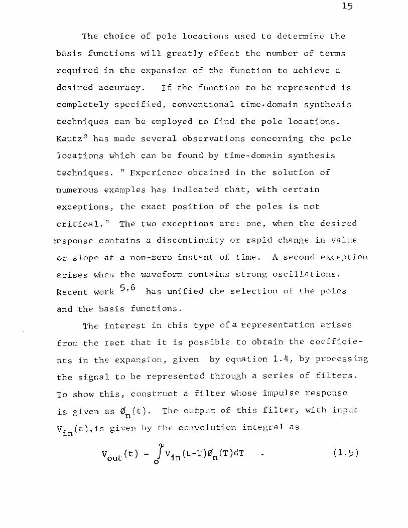
The choice of pole locations used to determine the
basis functions vJill greatly effect the number of terms
required in the expansion of the function to achieve a
desired accuracy. If the function to be represented is
completely specified_, conventional time·domain synthesis
techniques can be employed to find the pole locations.
Kautz 3 has made several observations concerning the pole
locations which can be found by time-domain synthesis
techniques. " Experience obtained in the solution of
numerous examples has indicated that_, \\1ith certain
exceptions_, the exact position of the poles is not
critical.'' The two exceptions are: one_, when the desired
response contains a discontinuity or rapid change in value
or slope at a non-zero instant of time. A second exception
arises when the waveform contains strong oscillations.
Recent work 5_, 6 has unified the selection of the poles
and the basis functions.
The interest in this type ofa representaticn arises
from the tact that it is possible to obtain the coefficie-
nts in the expansion_, given by equation 1.4_, by processing
the signal to be represented through a series of filters.
To show this_, construct a filter whose impulse response
is given as 011 ( t). The output of this fi 1 ter _, with inpu.t
v. (t)_,is given by the convolution integral as 1.11
V t(t) = Jv. (t-T)0 (T)dT ou· 0 1.11 n (1.5)

16
No-v1 if Vin(t) = f(-t) , where f(t) is the function to be
represented, the output of the filter at time t = 0 is
seen to be identical in form with equation 1.4 . Therefore
by applying a time-reversed signal f(-t) to the input
of a filter, whose impulse response is 0n(t) , and obser
ving the output of the filter at the epoch of the signal,
the coefficient of 0 (t) in the orthonormal basis function n
expansion of the input signal can be obtained.
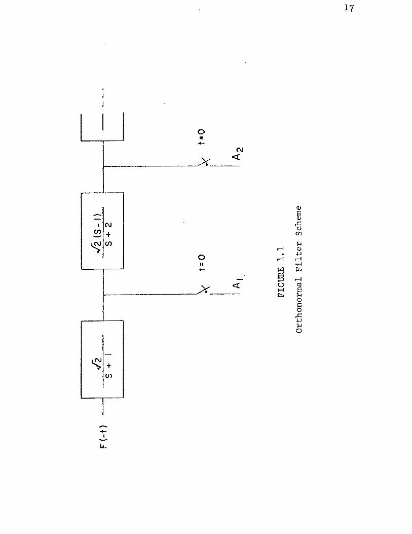
Consider again the pole set of the previous example.
The first two basis functions can be written as
The corresponding transforms are
F (S) = 2
2(~-ll TS+1lTs+21 =
This filtering and representation scheme described above,
also knovm as a Huggins spectrum Analyzer , is shown in
figure 1.1 • The A 1 s in this figure refer to equation
1.1 .
17
I
I
0 II - N
X <(
Q)
s Q)
,.c () (/)
$-I r-1 Q)
+J . r-1 ....... 0
II ·r-1
~ r:r~
r-1 -
co 0 s <{ H
$-I X
~ 0 s:: 0
,.c .u $-I 0
--I -

18
This type of a representation has been used advantage
ously in the representation of electrocardiograms7.
The selection of the exponential set and thus the determin-
ation of the pole locations was accomplished by a continual
adjustment of the parar,1eters until a good fit to the
input waveform was obtained.
The Huggins spectrum analyzer described above requires
that the input function be recorded in analog form and then
played backward in time through the filters. The determifr
ation of the epoch of the signal is a considerable problem
and much attention has been given to it. The filters
through which the signal must be processed require the
use of active devices or else 4 ter,minal networks.
It was the original recording of the signal which
was undesirable in the work started at Sandia Corporation+.
A secondary objective was to use filters which could
be completely passive. The recording of the signal can
be avoided by rewriting the expression for the convolution
integral as
00
Vout(t) = ofvin(T) 0n(t-T) dT
Thus the input signal could be occuring in real time.
However using the Kautz basis functions gives rise to
filters which are not realizable or else basis functions
which are not finite for large time.
:j: Sandia Corporation, Albuquerque,New Mexico Pr~me contractor to the A.E.C.

19
Work by Barnard and Bareruore 8 uses the filtering
concept, but applies it to a finite reconstruction interval·
The basis functions are the sums of positive exponentials,
orthonormal and well behaved in the mathematical sense
over the finite time interval. The resulting filters
are easily realized as three-terminal passive RC networks.
A typical waveform studied is shown in Figure 1.2 .
By sampling the output of 6 RC filters once every .1 sec.
this waveform was reconstructed with a maximum error of
less than 1 percent of the max~_m1..IDJ value of the signal.
The bandwidth and parameters of the original filters were
chosen experimentally and the error curve of figure 1.3
was obtained. This curve was unexplained in the original
work. Alpha is one of the parameters 'l;vhich determines
the bandwidth of the RC filters. The first attempts
at a general analysis of this signal theory systECm v;a.s to
relate the system parameters in some way to the bandwidth
of the input signal. This was done as the original
purpose of this system was to replace a sampled-data
acquisition system and thus equivalent parameters were
necessary. For a sampled-data system, the important
parameter is the highest frequency component of the input
signal.
This work has as its basic objective the det:ermL1ation
of the oasic parameters of this system in terms of the
properties of the input waveform to be represented.

20
8. 5 ====------ -------+-~,\=----+--------1---·---~= -_-----__ f--------+----
~---- ------1-------+--l-·--·\--\-+------ ------- '--- ------ ~----- ------
7.5 r------- -----jf--------H--+\-1-- r-·--
r------ -----+------ ---~\~----+-------J.-----+-----------r----- r--··------·
6.51-----+----+----t:f---+-+\-----l-----+-----f------t------r--~
---\\-+------ -------------- ----·-·-t-----·- ---------
s .s ~----4----·-+-------~------~- --r
··--------~--- ~-~- ---~---- -----r---·----·· -- ----,
'-' :~---f--------· ---->,._-~~~ -\- --- ---- ~--- -----= -~-~=~ -~= -1
3.51-------r------- ·------H----- \--- ---- ---- --- ·------1
----- =~---~-= -=-=-c- --K- -=~= ~ = --=--:_ -----~j .2.5~---·-
-. ----· ·-·------------------. ----------- --- ------ -------- __________ I 1. 5 ------- ----·-1--·--+--+------~-------- -------- -v-~--------- -l------------· ·------- ---- ------- ------ ----·--------·------ ---- -------r- --- -- -] --- ~-
U.51-·-- ~~~-:~===I ~::~=-==-----~tr ___ I:_ -~x-=:! -•J.5 --~-- . _=:I ________ ~.-.______ -- ___ _j _____ ~
u 0.1 ..;,2 u.3 0.4 o.5 o.6 u,7 o.a :.J.:l 1
Time (sec.)
FIGURE 1.2
Typical Signal to be Represented

L 0
g
M e a n
l 3 1 2
0
s -1 q u a -2 r e E -3 r r 0
r -4 ~--------~----~--~~~~~~----~--~~~~~~-----
. I alpha (a)
.3 .4 .5 .6 .7 .8.9 I.
FIGURE 1.3
Variation of Error With Alpha
3 4 5 6 78 910
1\) ~

22
CHAPTER II
BASIC SIGNAL THEORY SYSTEM
It is desired in this section to examine in more detail
the representation of a signal, F(t) , in a basis function
expansion. The basis functions are of the form
kat e--rr- . 0
(2. 1)
The approximation of F(t) in te~~s of the basis functions
is given as
,... F(t) = (2 .2)
with
F(t) ~ (t) w(t) dt n
where
w(t) = at/T
2ae 0
T (ea-1) 0
(2. 3)
Alpha (a) is a fixed constant, its selection is discussed
later. T is the sample period. 0
will approximate the signal F(t)
For a given N, F(t)
over the interval (o,T ) 0
with the minimum mean-square error. The coefficients,A n
in equation 2.3 will be obtained by sampling the outputs
of N passive RC filters every T0 seconds. T0 can also
be considered as the interval of reconstruction for the
signal F (t)

23
Figure 2.·1 shows the set of filters and the reconstruction
process.
To show how the RC filters are used to obtain the
coefficients A ~ define the impulse response, h (t) , n n
f h th . f 1 o t e n composLte i ter to be related to the basis
functions as follows
Equation 2.3 then becomes
To A = J F(t) h (T -t) dt . n n o
(2. 4)
However this is the form of the convolution integral
To .
f Vin(t) hn(T0 -t) dt 0
relating the input and the output, at time T0 , of a
network 'vith impulse response h (t). Thus the outpu.t of n
a filter with impulse response
h (t) = 0 (T -t) w(T -t) n n o o (2. 5)
is the same as the coefficient An in the expansion of the
function given in equation 2.2 . The impulse response
of the composite Nth filter is given as
h (t) = n (2. 6)

~-------l
j ¢o I rl h ~ Ao I 0 . I
l I I ; I I
F(t) I I h, H~ro~ I
hN composite filters with impulse response h(t)
t =To
I
yiN I •.
reconstruction
process
FIGURE 2.1
Block Diagram of Signal Theory System
{ 1: }-~(t)
1\) ,_. ..-
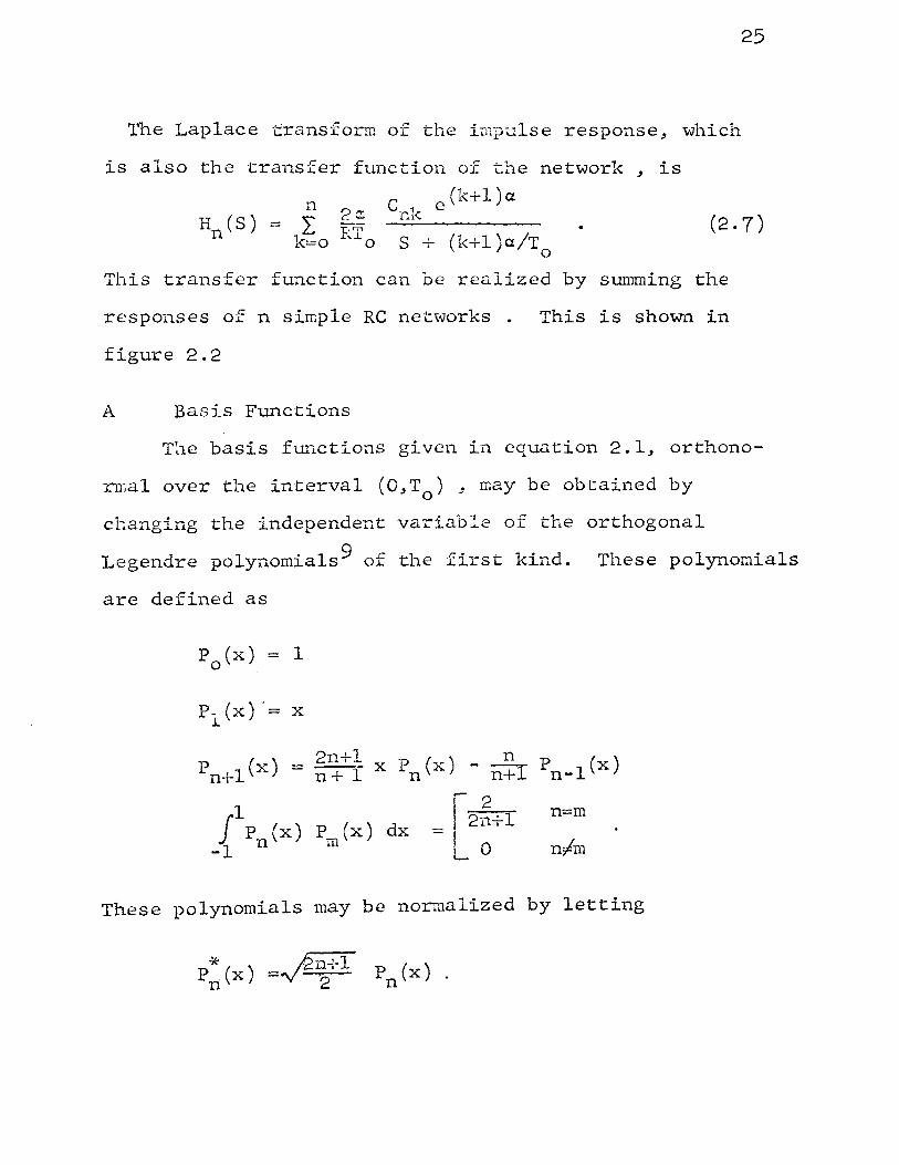
The Laplace transform of the impalse response, which
is also the transfer function of the network , is
n
25
H (S) = L 2o; n k=o RTo
C e(k+l)a nk
S + (k+l )a/T0
(2. 7)
This transfer function can be realized by summing the
responses of n simple RC networks . This is shown in
figure 2.2
A Basis Functions
T~e basis functions given in equation 2.1, orthono-
rmal over the interval (O,T0 ) , may be obtained by
changing the independent variable of the orthogonal
Legendre polynomials9 of the first kind. These polynomials
are defined as
P0 (x) = 1
P- (x) ·= X .L
pn+l(x) 2n+l ( ) n
pn-l(x) = n + 1 x p n x - n+l
1 = [2~+1 n=m
J Pn(x) P (x) dx nfm -1
m
These polynomials may be normalized by letting

I n s+.s _ - I I
F( t' I I St28
S+Cn~D,8
hh I
Ko
K,
Kn
FIGURE 2.2
Elements of a Composite Filter
An
!\) (J)

27
With this change in normalization~
1 ( p-x- (x) P* dx i n m
To represent a function in terms of the normalized
Legendre p'olynomials,
""' N F(x) = E Bn P~(x)
n=o
with
1 J F(x) P*(x) dx. -1 n
(2. 8)
The change in variables is given as: P*(x) , over the n
interval (-1~1)~ corresponds to 0 (t)~over the interval not eP - 1 and z -- R with x = 2z-l w(t) in
equation 2.3 comes from changing dx to dt in equation 2.8 .
In this notation and in the notation to follow
a ~ =
To
R a
1 = e - .
The first three basis functions are then:
0 0 ( t ) = 1/"'2
¢1 (t) =~ ~ ( 2e$t - ea - 1 )
02 (t) =/? ~2 ( 6e2~t - (12+6R)e.Bt +6R + 6 ) .
From equation 2.5 ~ which relates the impulse response
to the basis functions, the first three impulse responses
can be found.

28
= • .J1ofsea ( 6e2ae-3f3 t - (12+6R)eae-2f3 t
+ (R2 +6R+6 )e- f3 t ) .
B Filter Realizations
1. Parallel Realizations
The following example problem will show the parallel
realization of simple RC filters to obtain the impulse
responses given by the above equations. For numerical
convenience, the following values were chosen
!2 = = . 693
f3 = R
The basis functions then become
= 1/"""2
=A ( 2et - 3 ) 2

29
The impulse responseof the first three composite filters
aE then seen to be
=
=
-t e (2. 9a)
(2. 9b)
There are two ways to realize filters with these
impulse responsesJ in a parallel or cascade arrangement.
The parallel arrangement uses the fact that the impulse
response looks like the sum of the responses of several
elementary RC filters. This is sho\·m in detailJ for
this exampleJ in figure 2.3 . Figure 2.4 shows the
reconstruction of F(t) from the outputs of the composite
filters.
The cascade realization of the filters is obtained
by expanding the transformed impulse rE-sponses given
b · at· ~ 0 9 a ove 1n equ 10n~ c. •
= s + 1

l S+_l_
6
F( t) I V.( t)
S+ 3
FIGURE 2;3
Parallel Realization of Composite Filters
--Ao
--A,.
t~To A2
w 0

Ao [95o = .h.
A, ----i 0:=-A(ze'- 3)
A2 j¢.=JI(6e1-18e1 + 13) r FIGURE 2.4
Reconstruction of F(t)
F( t >
w I-I

(8+1)
(8+1) (8+2)
(8-7 /2 )2 + 15/4 H2 (8) = 2-/"10 ------
(S+l) (S+2) (8+3)
The zeros in the right-hand 8 plane could be realized
by lattices or by parallel ladders as in Guillemans 10
~rocedure. It is of some interest to observe that the
numerous additions and subtractions indicated in the
32
parallel realization would be done on a computer at the
time that f(t) is generated. Thus only the values at
the output of the RC filters at time t = T ~ desjgnated 0
here as V ~ need be recorded. n The cascade realization
does these computations_, so to speak_, with the components
in the filters. Considering component tolerances and
the resultant errors~ cascade realizations of this type
will not be considered further at this point.
The follOWing two examples are presented to help
clarify the steps involved.
EXAMPLE 1
Let F (t) t
-- e • This function is a linear combination
of 00 (t) and ¢1 (t) and thus a perfect reconstruction is
expected. Again choosing a= T0 = .693 _, the transfer
function of the RC filters become

33
1 1 1 ~ ~
s + 1 s + 2 s + 3
The input is F(S) = L(et) 1
= s - 1
The output of the nth RC filter is 1 1
Vn(s) 1'.+2 n+2 = s-1 S+n+l
2 1
n+.2 (n+2)2n+l
= 3/4
7/12
= 15/32
Performing the computations indicated in figure 2.3
gives the coefficients in the reconstruction as
Ao = 3/-J2
Al = 1/-J6
A2 = 0
Inserting these values into the computations indicated
in figure 2.4 gives the approximation of F(t) .

34
F ( t) = 3/2 + ( 1/2 ) ( 2 e t - 3 ) = t e = F(t)
This is the expected answer as F(t) was a component part
of 02 (t) .
EXAMPLE 2
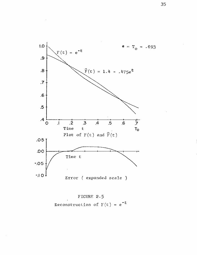
Let F(t) = e -t
This is a function which is seen
more often than the growing expoLential of the previous
example. Repeating similar procecures yields
vo = .3465 Ao = . 90
vl = .250 Al = -.1935
v2 = .1875 A2 = .0002
Neglecting the A2 02 term in the expansion gives the
following approximation of F(t).
~ t F(t) = 1.403 - .475e
Figure 2.5 compares the approximation to the actual
function. The error curve can be approximated with
triangles and using the fact that the mean-square value
of a triangle is .333 H2 ~ the mean square-error of this
approximation is found to be -726xl0- 3o
35
1.0 -t = e
a = T 0 = . 693
.9
.8 = 1.4 - .475et
.7
.6
.5
.4 ~------~----~---r--~-----4---~ 0 .I .2 .3 .4 .5 .6 .7
Time t To Plot of F(t) and F(t) .05l
.0 0 J---~----=;::::..___..,__ ____ -+-...=.....~;-----r-
Time t
-.05
-.10 Error ( expanded scale )
FIGURE 2.5
Reconstruction of F(t) = e -t

36
The mean-square value of the function can be found as
= .54
Thus the ratio of the mean-square error to the mean-square
value of the func·tion can be computed ·to be . 0015
2. Input - Output Realizations
It is possible to express the approximation of F(t)
in a form simpler than that given by equation 2.2 0
Equations 2.1 and 2.2 can be combined to give the approx
imation of F(t) in the following form
or
N F(t) = 2: An
n=o
F(t) =
~ C kct/T L k e o
k=o n
nat/T e o . (2. 10)
Figure 2o6 shows the relationship between the A coefficients
and the I coefficients for the case with a= T0 = .693
The coefficients given in equation 2.10 can also be
directly related to the outputs of the RC filters as
shown in Figure 2.7 . The input-output diagram in Figure 2.7
shows that the magnitude of the numbers which process the
outputs of the RC filters are the same. It is interesting
to examine a filter whose input is F(t) and whose output,
when sampled at t = T is the coefficient I in equation o n
2ol0 •

0 H
0 <{
H
+
('J <{
N H
~ ""--. -
~ <..0
(0 . C\l
~ t:!l H ~
3'{
~ H
~ ~ C'iS
<(.~
p Q) Q)
~ ~I <lJ
I=Q
p,.. •..-! ,..c; r:/l p 0
•..-! .u C'iS
.-I Q)
~

_ _._. __ I
S + I
F( t ) ls12 I I
S+3
~ 2.746 A
.. ~ -2.376
v. -{s~~Q-s
-EIWJ-- c
3~-A
V2 ---f:.::.:B a
~4~·c
- Vo I
I I
X v. I I I
f =To v2
c I 00 0
FIGURE 2.7
Input-Output Blo.:k Diagram
38
-F{t)

The transfer function ~K(S)~ of these filters can be
obtained by inspection of figure 2.7 0 The following
sketch shows the notation used with these transfer
functions.
Filter With
39
F(t) Transfer Function = ~(S)
--I t=T n
0
K0 (s) then becomes
or
[2.746
1000 s + 1
4.752
s + 2 +
3.120 l s + 3j
1.1482 + 4.0828 + 8.46
( S+l) (S+2) (S+3)
This filter has crnnplex zeros in the left-hand S plane
and can be realized as a RC filter11 . Computations for
K1 (s) and K2 (s) reveal the same form and although the
zero's are in the right-hand S plane~ they can be
realized as RC filters also.
C Multiple Sampling
The reconstruction of the function in the inter..ral
(O_,T ) has been shown in the previous two sections. To 0
reconstruct the function for more than one interval
requires some additional refinements. The asst~ption
made in the previous sections was that the filters
had no initial conditions stored on the capacitors
40
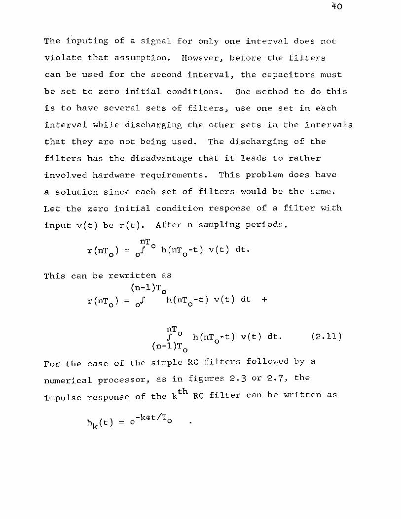
The inputing of a signal for only one interval does not
violate that assumption. However~ before the filters
can be used for the second interval~ the capacitors must
be set to zero initial conditions. One method to do this
is to have several sets of filters~ use one set in each
interval while discharging the other sets in the intervals
that they are not being used. The discharging of the
filters has the disadvantage that it leads to rather
involved hardware requirements. This problem does have
a solution since each set of filters would be the same.
Let the zero initial condition response of a filter with
input v(t) be r(t). After n sampling periods~
nT r(nT ) = J 0 h(nT -t) v(t) dto
0 0 0
This can be rewritten as
(n-l)T 0
r(nT0 ) = 0 J h(nT0 -t) v(t) dt +
nT 0 J h(nT 0 -t) v(t) dt.
(n-l)T 0
(2.11)
For the case of the simple RC filters followed by a
numerical processor~ as in figures 2.3 or 2.7~ the
impulse response of the kth RC filter can be written as

Now
-ka e h((n-l)T - t) 0
and therefore equation 2.11 can be written as
nT
41
J 0 h(nT -t) v(t) dt. (n-l)T0 °
(2 .12)
The integral on the right in equation 2.12 is the
response of the kth RC filter at the end of the nth
sampling interval based on zero initial conditions
at the ber_inning of that interval. Therefore one
set of filters sampled every T0 seconds is sufficient
to implement the multiple sampling scheme.

42
CHAPTER III
DERIVATIVE APPROXIHATION OF THE SIGNAL
A Derivation of Results
In each sample interval~ the signal reconstruction
is independent of previous reconstructions. Thus there
is no assurance that the complete approximation will
be continous at the sample points. If the derivative of
the signal~ F'(t): is approximated by the output of
the composite filters~ then a simple integration of this
output will yield a continous approximation of F(t) •
Approximation of the derivative of F(t) requires only
a change in the num·erical processing of the output of
the simple RC filters. The derivative approximation
starts with
F' (t) = 00
l: d 0 (t) n n n=o
where dn is defined as
T
J °F' (t) 0n(t) w(t) dt • 0
The response of the nth filter with impulse response hn(t)
and input F'(t) is given as
V (T ) = n' o
To j F' (T) hn(T0 -T) dT • 0

This can also be \vritten as
To Vn(T0 ) = f F'(T0 -T) hn(T) dT.
0
In general
t = I F(T) h (t-T) dT
o n
or
and by Leibnitz's rule
t
43
(3.1)
dvn(t)
dt = J F (T) h~ ( t -T ) dT + F(t) h (0) (3.2) n 0
and
&t t
j F'(t-T) hn(T) dT 0
+ F(O) h (t) n --=
The last integral can also be written from equation 3.1 as
(3.3) dt
Equating equations 3.2 and 3.3 gives
t Vn(t) = 1 F(T) h~(t-T) dT + F(t) hn(O)
0
If h (T -t) = 0n(t) w(t) ~ equation 3.4 can be written n o
as To
dn = V (T) = J F(t) h 1 (T -t) dt n o 0 n o
+F(T0 ) hn(O) - F(O) hn(T0 ). (3.5)

44
Equation 3.5 shows that with the addition of the
"\7 3 lue of the input 'l:vaveforrn at the sample points., the
derivative of the input waveform can be approximo.ted by
the expression given in equation 3.5 . The impulse
responses of the composite filters change., but an
observation of h 1 (t) shows it to be of the same form n
as hn(t) •
B Filter Realizations
Examining equation 3.5 fo·.c d 0 gives the following
To d = 21 J F(t) h' (T -t) dt + F(T0 ) h 0 (0)
0 0 0 0
h (t) 0
""'C: a c:. e ho(O) = RTo
e -{3t h 1 (t) = 0
-/Jt e
Dn(S) will signify the transfer function bet'l:veen F(t) 2.nd
the coefficient dn as shown in the following sketch.
F (t) -----t
Filter With
Transfer Function = Dn(S)
L----------------------------·--D0 (S) is then given as
a ae RTO
t==T 0
d n
45
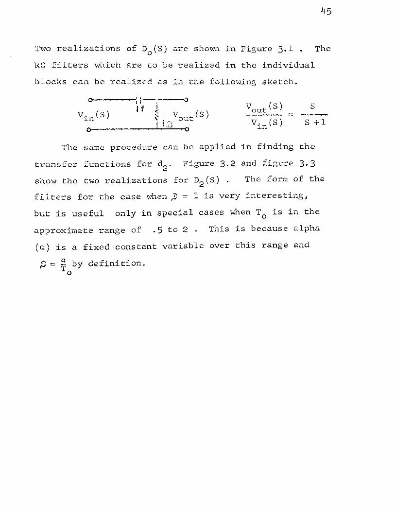
Two realiza-tions of D0 (S) o.re shown in Figure 3. 1 . The
RC filters which are to be realized in the individual
blocks can be realized as in the following sketch.
0 \~ 0 I i l Vout(S) I •f s vin(s) s V (S) <" o-,r- =
I i ·. --~.._ vin(S) s +1 .~,
0 I •:,J 0
The same procedure can be applied in finding the
t ,- - ..f-. .c , ransrer runc~~ons ~or a 2 . Figure 3.2 and figure 3-3
snow the two realizations for D2 (s) . The form of the
filters for the case when ~ = 1 is very interesting,
but is useful only in special cases when T0 is in the
ap?roximate range of .5 to 2 . This is because alpha
(a) is a fixed constant variable over this range and
p = ~ by definition. To

<o..
CQ + CJ)
T
0 ·a
0 OJ 0::
CQ.
I ---l.L
0
0 "'0
Q) a::
,_o II -
C/) + (/)
---LL
1~6
...--.. C/) ....__..
0 (::l
4-1 0
...-I . U) (Y) t::
0
~ ·~ .w m
c.!) N II H •rl
~ r-1 Cll. m
<l)
~
0 ;:3.:
(-1

I I X I l S+l: :---; 13
2 I .......... I 3 6 S+ 2 I I
I I I
F( t) I I
-~ r---~~
3 I 2 4 5+3 I
:t= To
FIGURE 3,2
Realization of D2 (s)
~ ..L. ,-
( L l-B-d2
~ /_._
-+= ......:j

I I s 5+ -~] f ~-- 13 1
s F(t) I I S+2
s S+3
~ 36 I I
I I
I
't=To 24
FIGURE 3.3
Alternate Realization of D2 (S)
10
[3 = I
d2
-+= OJ
CHAPTER IV
DETZRMINATION OF ALPP~
The system has been discussed as to its operation
a:.1.d how the basis functions are forr.-:ed_, however the
parameters of the system have not yet been determined.
These parameters are : a_, T0 _, N . These parameters
will be selected to minimize the reconstruction error
of the system approximation for some class of input
r.vz~ ve form.
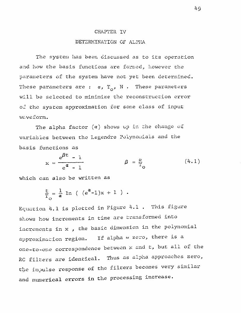
The alpha factor (a) shows ~p in the change of
variables between the Legendre Polynor.1ials and the
basis functions as
49
e/3t - l (4.1) X=
which can also be written as
t 1 a T = a ln ( ( e -1 )x + 1 )
0
E<;lua·tion 4. 1 is plotted in Figure 4.1 . This fig·u.re
shows how increments in time are -~ransformed into
increments in x _, the basic dimension in the polynomial
approximation region. If alpha = ze~o_, there is a
one-to-one correspondence between x and t, but all of the
RC filters are identical. Thus as alpha approaches zero,
t~e impulse response of the filters becomes very similar
and numerical errors in the processing increase.

1.0
.8
.6
.4
.2
X 0
-.2
-.4
-.6
-.8
-1.0
a =
-~ .3 -~
FIGURE 4.1
Relationship Between x and t as a Function of Alpha
50
.8 1.'o

51
If alpha becomes very large, increrr e t · t · 1 1 n s 1n une ~ecome
very nonlinearly transformed into increments in x and
again numerical troubles '1"·'1.11 arise. Thus alpha is
seen to be a conversion factor and should be in the range
of0.5 to 2.0. This increase in error for large or small
alpha , as sho,,m experimentally in figure 1. 3 , r.·as
unexplained in the previous -v•ork by the author8 . Figure
4.2 sho~s the variation of the mean-square error of
the reconstruction as a function of the nt.m1ber of terms
in the series and as a function of alpha. The results
for this figure were taken from a computer simulation
at Sandia Corporation of the complete signal theory
system. This system simulated the simple RC filters,
generated the basis functions and computed the reconstru-
ctions. The basis functions were generated by a Gram-
Schmidt procedure. This procedure gave rise to numerical
troubles as N increased and thus the generation of the
basis functions by the method described in chapter 2 vJas
developed. As a result of the inaccurate generation
of the basis functions, it is most likely that the errors
for large N are due to nQ~erical problems of the original
simulation. Theoretically the error -v•ill approach
zero as N becomes very large. The increase in error
for decreasing N can be interperted as truncation error
due to an insufficient nwnber of terms in the approximation.

52
0
L 0
g -I
M e a n
s -2 q u a r e
-3 E r r 0
r -4
4 6 8 10 12
Number of Filters
FIGURE 4.2
Error Vs. N and Alpha

Figure 4.2 tends to verify the previous range of
alpha T~th alpha equal to 1. appearing to be about
the optimem value.
Conceptually it can be seen that the filters are
merely a means to obtain the coefficients in the basis
function expansion and the filtering of the T.·aveform
caused by these filters is of no significance.
that the band'·'idth of the simple RC filters is
Recall
na/T , 0
~--here n is the number of the filter and T is the 0
sample interval.
Since alpha has been determined: this leaves tvo
parameters to choose. N and T . N is the number of 0
53
terms in the expansion and is also the number of filters
required. T is the sample interval and the interval 0
of reconstruction. To determine these tvo parameters,
a typical input to the system will be classified in such
a manner that variations from this typical input T-·ill
not affect the accurate reconstruction of the input
signal. T~u methods to classify the input signals are
presented in the follo,.··ing ,..-ark, one a graphical technique
and the other requiring a kno~ledge of the pole locations
of the input signal to classify the signal.
54
CHAPTER V
GRA~1ICAL CLASSIFICATION OF INPUT SIGNALS
A Polynomial Approximation
Since the basis functions are obtained from a trans-
form applied to the Legendre polynomials~ this work will
be based on the Legendre p'olyno:.:nials in order to reduce
the tedious calculations which would arise if the ortho-
normal basis fu._"'"lctions were used. The results are easily
changed to the basis functions.
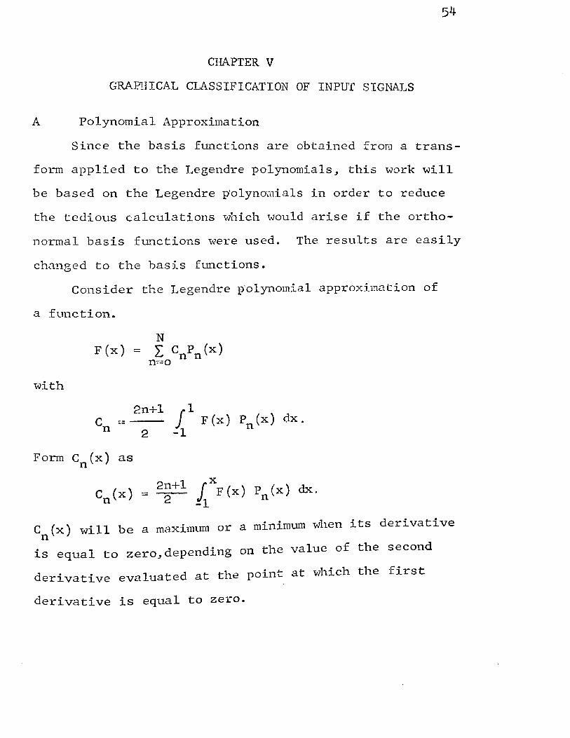
Consider the Legendre p'olynomial approximation of
a function.
N F(x) = L CnPn(x)
with
Form C (x) as n
n=o
2n+l
2
1 1 F (X) P (X) dx . -1 n
Cn(x) will be a maximum or a rninimwn when its derivative
d d . on the value of the second is equal to zero~ epen ~ng
derivative evaluated at the point at which the first
derivative is equal to zero.
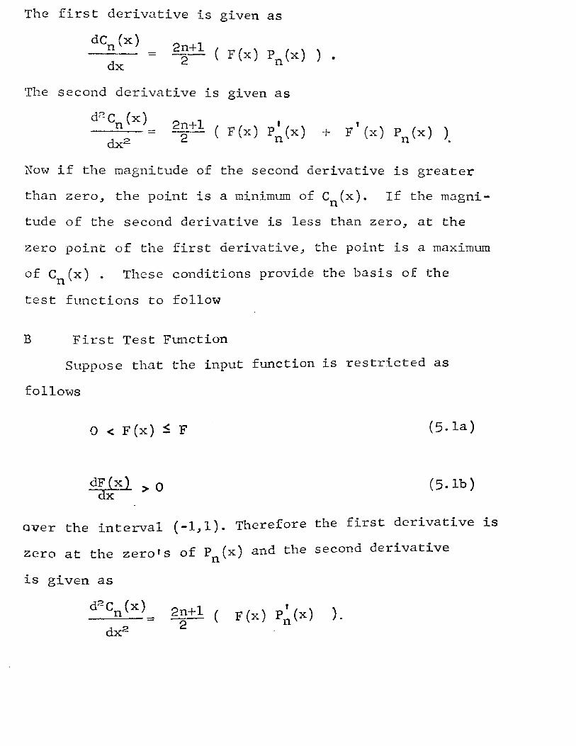
The first derivative is given as
The second derivative is given as
' + F (x) P (x) ) n . -----
Now if the magnitude of the second derivative is greater
than zero~ the point is a minimum of C (x). n If the magni-
tude of the second derivative is less than zero~ at the
zero point of the first derivative~ the point is a maximum
of Cn(x) . These conditions provide the basis of the
test functions to follow
B First Test Fm1ction
Suppose that the input function is restricted as
follows
0 < F (x) ~ F (5.la)
(5.lb)
over the interval (-1~1). Therefore the first derivative is
zero at the zero's of p (x) and the second derivative n
is given as
d 2 C (x) ----'-n.;;..___ - 2n+l (
2
f F(x) P0 (x) ) .
56
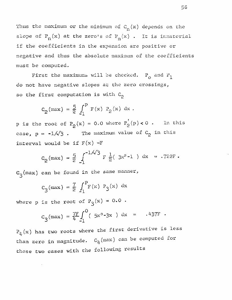
Thus the maximum or the minimwn of C (x) depends on the n
slo?e of Pn(x) at the zero's of Pn(x) . It is ir..~naterial
if the coefficients in the expansion are positive or
negative and thus the absolute maxim~~ of the coefficients
must be computed.
First the maximumb will oe checked. P0 and P1
do not have negative slopes at the zero crossings~
so the first computation is with c 2
c2 (max) = ~ Jp F (x) p fx) dx . 2 \ -.L
I
p is the root of P2 (x) = OoO where P2 (p)<0 In this
case~ p = -1/~3 . The maximum value of c2 in this
interval would be if F(x) =F
__ r-1/~3 c2(max) = ~ _{
c 3 (max) can be found in the same manner~
C- (max ) = r 1 p F (X ) P 3 (X) dx j -1
where p is the root of P3 (x) = 0.0 ·
0 C (max) = J!- J ( 5x3 -3X ) dx
3 -1 =
= . 722F •
.437F .
Pb(x) has two roots where the first derivative is less t
than zero in magnitude. C4(max) can be computed for
these two cases with the following results

57
= -371F
and
gp [ -. 8611 C4(max) = ~ P4(x) dx = .276F .
-1
Taking the largest of these two gives c4 (max) = -371F •
This same procedure can be applied to find the
minimum value of the coefficients. In this case, the
value of p is where the polynomial has a zero crossing
with positive slope. Table I compares the maximum and
minimum values of the coefficients as a function of N .
It is seen that the maximum value of the coefficients
comes from using C (max) in each case. These values n
are plotted in figure 5.1 This figure reveals that
To make use of this expression for Cn,
it is necessary to examine the mean square error.
F(x) can be expressed as two series,
F(x) 00
+ L _CnPn(x) • n=N+l
The first N terms representing the approximation and
the remainder of the terms representing the error.
The mean square error can be evaluated as
f l ....... • 5 ( F ( x) - F ( x) ) 2 dx
-1 =
00 r CnPn (x) )2dx. n=N+l

TABLE I
MA.XTMUM AND MINIMUM VALUES OF C vs. N n
N Cn(min) C (max) n 1 -375F
2 .481F • 'T22F
3 -350F .437F
4 -371F
58

I. I j 1.0 l .9
.s
.7 Cn (max)
.6
.5
.4
/
N=2
FIGURE 5.1
C (max) vs. N for n
First Test Function
N-'2 -v N=4
IJ1 \0

Expanding the square in the right-hand integral yields
co
L CnPn(x) n=N+l
= 00
L C 2 P 2 (x) n=N+l n n
+ L cross terms
60
Integrating over the period makes the cross terms drop
out due to the orthogonality of the Legendre polynomials.
The orthogonality also makes
1 J p 2 (x) dx -1 n
= 2 2n+l-
and the expression for the mean-square error (MSE) can
be written as
MSE 00 11 -- . 5 2: Cn 2 P2 (X) dx
n=N+l -1 n
00
MSE- L n=N+l
c 2 n
2n.+r •
Substituting the bound on en~ 1.47F I n gives the final
C?XIJression for the HSE as
=
00
r n=N+l
1 MSE T2n+l)nz- • (5. 2)
Th g ;\ren by equation 5· 2 has been e mean-square error ~
tabulated as a fwtction of N in table II
Equation 5.2 relates the mean-square error of the approxi-
mation only as a function of the number of terms (N)
used in the approximation.

TABLE II
MEAN-SQUARE ERROR vs. N
N MSE
2 .0738
3 . 0395
4 .0245
5 .0166
61
62
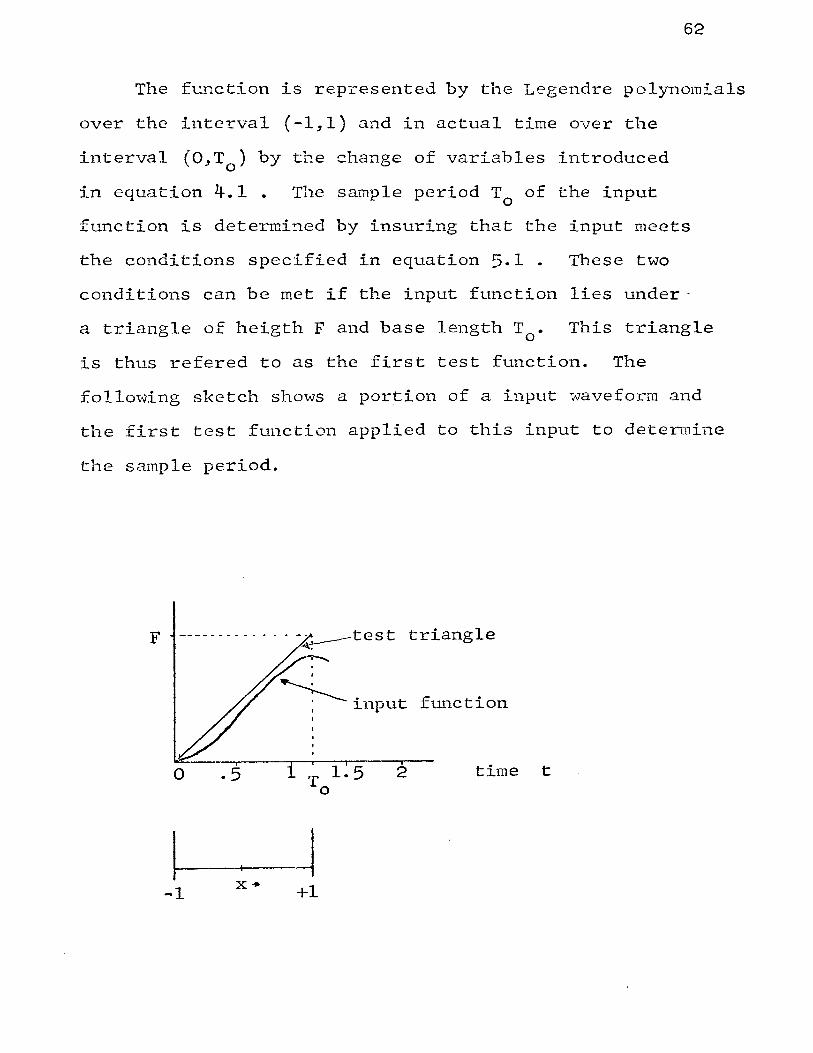
The function is represented by the Legendre polynomials
over the interval (-1,1) and in actual time over the
interval (O,T0 ) by the change of variables introduced
in equation 4.1 . The sample period T0 of the input
function is determined by insuring that the input n1eets
the conditions specified in equation 5.1 . These two
conditions can be met if the input function lies under·
a triangle of heigth F and base length T0 • This triangle
is thus refered to as the first test function. The
following sketch shows a portion of a input waveform and
the first test function applied to this input to de·termine
the sample period.
F --------------- test triangle ~
I
~input function
- I i 1~5 I
time 0 .s To
2 t
I ~ -1
x-. +1

This sketch shows that the real-time sample would be
required at ~ 1.2 seconds in order to reconstruct the
63
function over this interval. For multiple sampling, i.e.
reconstruction over several intervals, the shortest
interval found in a waveform would be the sampling period
required for the entire waveform.
This graphical technique thus provides a rapid
estimate of the sampling rate and the mean-square error
in the approximation. It is of interest however to
be able to compare the error to the input function.
Since the straight-line test function only bounds the
input function, there is no w.3.y to exactly specify the
mean-square value (MSV) of the input function. An
approximate value of the MSV can be obtained by assuming
that the input function is approximately the test function.
Thus the }~V of the input is approximately the MSV of
the test fm1ction, which is a triangle of height F and
base length
MSV
T in the polynomial region is the distance between -1 0
and 1 or T = 2. 0
Thus the ratio of the MSE to the MSV
of a function which fits under this first test function
can be specified. This is given in table III.

64
TABLE III
RATIO OF MSE TO MSV vs. N
N MSE M:sv
2 .221
3 .119
4 .0735
5 .050
,

65
These results from the Legendre polynomial approxi-
mation of a function can be applied directly to the basis
function expansion of the signal. The first test function
is derived from P1 (x) = x with a shift in the average .L
value of F/2 . Thus figure 4.1 , which shows changes
in x to changes in t as a function of alpha, is seen to
also be relating what the test function should appear as
in the time-domain associated with the basis functions.
For the range of alpha of .5 to 2., which was selected
in Chapter 4 to .avoid numerical troubles, it can be
seen that the triangle test func~ion in x is approximately
still a triangle in the time domain.
It is to be observed that si~ice the tes·t func·::ion
bounds only the magnitude of the coefficients, the
following sets of specifications on the input waveform
are ider;.ti.cal.
O~F(t):SF
02:F(t)2; F
dFlEJ.. > O dt
d:?J.tl <0 dt
all x in (-1,1)
all x in (-1,1)
Tfuds is equivalent to having a triangle going negative
in time or else folded on itself.

C Second Test Flli1Ction
The second test function is derived from the
Legendre polynomial ~ P2 (x) = ~( 3x2 -l) 0 After
a shift in values~ this test function appears as
a isosceles triangle of altitude F and base 2. It
has a slope of F also. All functions lying under this
triangle with a first derivative equal to zero only
once in this interval are included as functions which
can be covered by the second test function. A sketch
is shown belo'tv to clarify this case.
_s test function - s;- input signal
F
-1 1
66
The procedure to fj_nd the maximum value of the coefficients
is the same as in the previous test function. In this
case however the maximum input is assumed to be the
second test function instead of just a maximum-value
of F.

67
The actual computations of the values of the coeffici
ents will not be shown here but are given in tabular
form in Table IV It is noticed that c3 does not
seem to fit into the same pattern that c2 and c4 are forming. This is because if the input function
is symmetric ~ the odd terms will not exist in the
expansion. The maximum values of the C's only were
listed in this table. The table stops at N = 4 due
to the complexity and tedious calculations. Plotting
these values of C (max) on log-log paper in Figure 5.2 n
reveals that the expression for Cn(max) can be given
as
The mean-square error for the second test function
can be found using the previous calculations for MSE.
MSE = 00
>: n=N+l
2
2Cn 2n+l ·
or the MSE for the second test function is
MSE = 00
1.21F2 r n=N+l
1 ( 1) ·362 . 2n+ n (5.3)
I F2 for the first and second Figure 5.3 plots the MSE
test functions and for the case if each of the coefficients
were equal to a constant F •

TABLE IV
MAXINUM VALUES OF en vs. N
N
2
3
4
r en (max) 1
.689F
.437F
• 605F
68

69
'¢ II ---------4:---
Z
r<> II --------1---------Z:
!=: H 0 0 •M
4-1 w C\J z CJ
~ N
. ;j 1..!"\ ~
II (/)
z ~ :> w
(/,) ....--... Q) 0 ~ E-1 H ro J:I.t !3 ·-o .___
~ !=: 0
0 CJ Q)
Cl)
CD . I c: tO 1'-.
-X 0 E -
0 (1) tO 1'- (!) LO c: . (J

:t-'J.SE
p2
70
7
5 C - F-
n r---r--t--+--~-4
3
2
Second Test
.a Function
.7
.G -----.5
.4
.3
.2 First
Test Ft:!.l1ction
_,
.02
.OIJ------------------L---------~----~~--~----~-----
N = 2
FIGURE 5.3 MSE vs. N ---p
3 4 5 6

71
The convergence of the second test function is not
sufficiently different from the case with each coeffic-
ient set equal to a constant to consider the possibility
of including another test function in the discussion.
One reason that the test functions specify so many
terms to reduce the MSE/NSV ratio to acceptable values
is that the test functions cannot distinguish be·tween
functions with an infinite nu.1.11ber of terms in their
power series expansi<::>ns and those vvith only a few terms.
Consider the following t\..JO example inputs.
with x in the interval (-1~1) . Both of these examples
appear identical in form and satisify the requirements
set do\·m i.n equation 5.1 for the first test function.
However £ 1 \-Jill require many rno·re terms to represent
it than f 2 which only requires three terms in its
power series expansion. The inability of the test functions
to distinguish between these types of functions is one
of the principal disadvantages of the graphical classifi-
cation scheme.
The second test function will allow a slower sampling
rate than the first test f~~ction.

72
Howeve~ to achieve the same accuracy with the second test
function, Figure 5.3 shows that it will require many
more filters. Thus,the total number of data points
needed to represent the function increases when using
the second test function instead of the first test function.
The chapter on problems for further study has some concepts
which were not fully investigated, but which could make
the second test function competitive with the first test
function by allowing a much closer fit to the waveform
and at the same time specifying a long sample interval.
A final disadvantage with this system of classifying
the input waveform comes form the fact that to have a
MSE /MSV ratio of . 05 requires five terms ( v'ith the
first test function ) reg.ardless of how the sampling
rate is changed. Thus, sampling faster than is specified
by the test function will not reduce the number of terms
required. To overcome this inherent conservative nature,
an entirely different concept is presented in the next
chapter.

73
CHAPTER VI
CLASSIFICATION OF INPUT SIGNAL BY POLE LOCATION
A Error Analysis
The input signal can be classified in terms of its
general pole location in the complex S plane. One pair of
polroJlocated at S = -a ± jb, can be considered to be
due to a general function of time
f(t) = A e-at sin (bt+A). (6. 1 )
A i.s an arbitrary amplitude constant and A is a arbitrary
phase constant ,..;hich depend on initial conditions.
For a given maximum error, which depends on N , this
function can be represented over the interval (O,T 0 ) as
1"-
f(t) -N r (6. 2)
n=o
If it is desired to represent the function in equation
6.1 over the interval T0 ~ t ~ 2T0 , it is necessary
to know ~1at conditions exist to keep N from changing.
Defining t' = t - T then tt is defined over the 0,
interval (O,T0 ) • The function of t' defined over this
new interval can be written as
f(t') = f(t)f =A e-a(t'+To) * t=t'+T
0

which can be rewritten as
f(t')
or finally as
-aT -at' = A e o e
74
sin (bt I + (bT +'A)) 0
f(t 1 )- Be-at' sin (bt' +'!')_, (6.3)
with B = Ae-aTo and 'i" = bT 0 +'A Equation 6.3 is
identical in from with equation 6.1_, but with different
amplitude and phase constants. Thus if equation 6.1
can be represented over the interval (O,T 0 ) with a
given value of N_, which is independent of A and 'A_,
then the function in equation 6.1 can be represented ,
with the same relative error, over any T interval by 0
a series with the same number of terms.
The error in equation 6.2, due to truncating the
series with N terms_, can be dete~~ined as follows:
define
-1 b tan a
The following sketch shows these parameters.

75
Complex S Plane jW
jb
0
J -a 0
The following two series from Jolley12 are based on this
notation.
eat cos(bt) =
eat sin(bt) =
; i£t~ ~ n!
n=o
~ ~)n ~ n!
n=o
Equation 6.1 can be rewritten as
cos (n0).
sin (n0).
f(t) = A cos('A) e-at sin(bt)
+A sin('A) e-at cos(bt)
(6. 4)
(6. 5)
(6. 6)
Substituting equations 6.4 and 6.5 into equation 6.6 gives
oo (nrf~ { } f(t) =A L cos('A)sin(n0) + sin('A)cos(n0) n=o
or
f(t) = A ~ ~f)n n=o
sin ('A+n0),

76
The function given in equation 6.1 will be approximated
over the. interval Substituting t = T into 0
equation 6.7 and truncating the series at n = N terms
\vill give a bound on the error as
oo (rT0 ) 0
r errorf ~ A L n=N+l n!
This can be rewritten as
(rT )N+l r error I' S A 0 { 1 +
(N+l) 1
or
(rT )N+l f error f :S A 0 { 1 +
(N+l) l
Vih.ich can be expressed as
A (rTo)N+l ferrorf S - T
(N+l) I ( 1 ... \ 0 )
(Tor)2 } ---· + ..,.. ...
+
(N+2.) (N+3)
(rT )2
_ __;0;;;..___ +. . . . } N2
(6. 8)
If the !error! is constrained to be less than some
small percentage ~ of A~ the maximum possible value of
the function given in equation 6.1, the following
expression arises
(rT )N+l ---
(N+ 1 ) ! ( 1 - rio ) "1 > (6. 9)
This expression for the error is inde~endent of A
and A, a condition required at the end of Equation 6.3 .
For a given value of N and T0 , lines of constant error
are represented by lines of constant r~ or circles in
the complex S plane.

77
Figures 6.1 and 6.2 sho-.;v these lines of constant error
as a function of N. The significance of these graphs
is that if a pole location is known for some input functionJ
this graph shows the number of terms needed in an expansion
of the ~orrn given in equation 6.2 . This expansion being
for the given value of maximum error.
For the case when the input function contains
several poles, the general error expression can be
developed from Heavisides partial fraction expansion of
the function. This expansion shows that the composite
time function is the s~mple s~~ of the time responses
due to each pole contained in the ir.put function. Thus
the error can be written as
(T )N+2 [ A rN+l N--t-1
Jerror]S 0 1 l +
A2r2 +
(1-~) r T . . . (N+l) 1 (1-p)
Anr~+l J + .,... ,..,.,
(1-"'"~Lo)
for the case when the input contains N poles. ( NoteJ
although complex poles are really two poles, this work
consiriers them as just one pole at distance r from the
origin of the S plane. See equation 6.1 for the form
of the general time response.) Letting the kth pole
represent the pole most distant from the origin, this
expression can be ~~itten

~ 5
4 I . 98
5 1.12
6 1.32
Complex s
Plane
T0 normalized to one second N = 7
-2
FIGURE 6.1
Pole Location vs. N for ~ =.Ol
j2
I'W IJ
/ ~ ___J.jl
cr
~ (X)
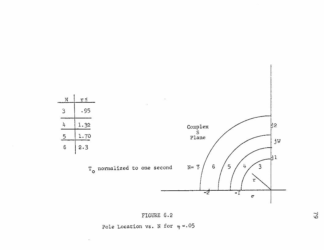
N Lti_ 3 I .95 -4 I 1. 32 Complex
s 5 I 1. 70 Plane
6 I 2. 3
T0 normalized to one second N~ Y,
FIGURE 6.2
Pole Location vs. N for ., =. 05
/
I ~
(]'
1<12
:jw
-..::)
\0

80
r error[ ~ (N+l)l (l-rkT0 /N)
+ ... +
A N+l (1-- T I ' r n-. { rn} { ~1 1. N; } l Ak) rk TI=~~ ~<To IN)
n o (6.10)
From this expression~ it is seen that if one pole is at
a much greater distance rom the origin than the other
poles~ the error caused by the other poles is almost
negilible compc:red to this pole. Thus the "dominant"
po~e in this error expression is the pole which is at
the greatest radius from the origin of the S plane.
If the input fw1ction contained a repeated pole~
a corresponding time function would appear as
f(t) =A t -at e sin (bt+'A) ..
The resulting error expression car. easily be seen to be
AT ( rT '.N+l 0 .... 0)
r error[=:- (6.11) (N+l) I ( 1-rT 0 /:-J)
which is merely T0 times the error due to a sing~e pole
at that location.
The po\Jer series expansion in t, given in ecuat:ion ..
6.2 ~ can be changed into a basis function expansio~ of
the function in 0. (t) by the following change in variables. n

81
X + 1 t =
2
with t in the interval (O,T0 ) and x in the interval (-1,1).
Then it is possible to write
N f(t) = L A tn
n=o n =
This can be expressed as
f(t) =
A basic relationship between the power series in x
and the Legendre ~olynomials is13
n X
n = L d P (x)
m==o m m
Thus f(t) can be expressed in general as
N f ( t ) = L Hm P m (x ( t ) ) •
m=o
Now Pm(x) is transformed into the basis functions by
the change in variables
at/T 1 e o -X == 2 - 1 a
e - 1
( 6. 12)
6r it is possible to express f(t) in terms of the basis
functions as
f(t) == (6.13)

82
The derivation leading up to equation 6.13 sho'~
that f(t) can be expressed in a basis function expansion
with the same nu..'Tiber of terms required in the power series
expansion. As a result, the circles of constant error
shovm in figures 6. 1 and 6. 2 can be applied directly to
a basis function representation of the input signal.
This section has shown that a knowledge of the poles
of the input signal is sufficient to choosethe sampling
rate and the number of terms required in the basis
function expansion of the input signal. To eliminate
some of the interaction between T0 and N , fix the sampling
interval T· at on~.se~6nrl. Now if the poles of the input 0
function are at such a distance from the origin of the S
plane that an excessive ntunber of tenus are required,
time scale the input signal by some constant c, ie
let t be replaced by ct . Then samples of the input
will occur every 1/c seconds and the frequency components
of the input waveform will then be reduced by the same
1/c factor. The resultant effect is to move the poles
toward the origin until. an acceptable error is obtained.
The final trade offbetween sampling rate and number of
tenns can only be solved by the introduction of some
other criterion such as hardware limitations. As a rule
of thlli~b, the number of terms should not exceed ~ive or
six since each t:erm requires an additional filter in
the complete system.

B Determination of Pole Locations
1. Time-Domain Synthesis
The pole locations of the input function in the
complex S plane can be determined by time-domain S)mthesis
procedures. There a.re many techniques listed in the
literacure and in the two discussed in this workJ the
following notation will be used. y~ = y*(t=t.) denotes ~ ~
the approximate value at time t = ti = T0 + i fl t .
T0 denotes the starting time, usually assumed to be zero,
and .6t denotes the time increment between data points.
y. ~vill signify the input values at the same time. ~
Fundamental to all of the time-domain synthesis
techniques is the minimmn mean-square error approximation
for a finite set of data points.
by a set of basis functions 0.(t.) J ~
y~ will be approximated ~
( these basis functions
are not the same as defined earlier in equation 2.1) as
y~ = ~
m
l: j=O
a~ 0. ( t.) J J ~
i= 1,2, ... n. (6.14)
m denotes the order of the approximation and n denotes
the last data point. There are n-1 data points.
m · t b d term'11ed so tl1.at the weighted mean-square a. ~s o e e ~ J
error

84
n m n ;~_,J1 w(ti) [ Yi - E amJ. 0J. (t; )]2 = L T.v. R::; (6.15) ~ j=o ~ i=l ~ ~
is minimized. '\v ( t . ) - w. is the weight function and ~ ~
R. is called the residual a-t t .. The superscript ~ ~ m
denotes the fact on a. that the coefficient will g
generally depend on m. To calculate the a~'s~ the J
partial derivative of equation 6.15 with respect to ltl
ak is set equal to zero.
-2 n L w. (y. -
. 1 ~ ~ ~=
m r a~ 0.(t. )] 0k(t.) = 0
j=o J J ~ L ( 6. 16 )
k = 0~1~2~ ... m
This system of m+l linear equations is called the normal
equations. Solving this system of equations for the
coefficients ai? allows the function to be approximated J
as given above in equation 6.14. If the 0.(t.) are J L
an orthogonal set~ the coefficients are independent
of m. The off-diagonal terms in the normal equation
rnatri){ become zero. Thus a~ becomes a. if the basis J J
functions are orthogonal. These are the basic steps
in all mean-square error approximations
Th Y 14 t" d · th · me·~...~hod ;s presented e engst -1me- oma1n syn es:ts . -'-
to show the standard procedure of solving for the poles
of the input function.
85
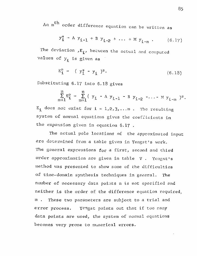
th An m order difference equation can be written as
Y1 =A Y1.·-1 + B y1.._2 + ... + M )' i-m · (6.1'{)
The deviation ,Ei, between the actual and computed
values of y. is given as 1.
Substituting 6.17 into 6.18 gives
n L E~ ·
m+l J..
n L (
m+l v. J 1.
E. does no·L.·- ~x1."st for 1." 1 2 3 m 1. --- == , , , • • • •
(6.18)
The resulting
system of normal equations gives the coefficients in
the expansion given in equation 6.17 .
The actual pole locations nf the approximated input
are determined from a table given in Yengstts work.
The general expressions for a first, second and third
order approximation are given in table V . Yengstts
method was presented to show some of the difficulties
of time-domain synthesis techniques in ge11eral. The
nwnber of necessary data poi~ts n is not specified and
neither is the order of the difference equation required,
m . These two parameters are subject to a trial and
error process. yengst points out that if too w.any
data points are used, the system of normal equations
becomes very prone to numerical errors.

86
TABLE V
POLE LOCATIONS FROM YENGST 1'-1ETHOD
Order of Difference Equation Relationship of Parameters y-x-cs)
K First Order
Second Order
Third Order
e -a !J. t = A
-a .6 t e
~b !J. t e
= ~ + ~(A2 +1lB} 2
= A - J""(A2+l~ )' 2
e -a !1 t - E + F + ~
S +a
-b 6t E+F I {E-:[}Q A e = - "2 -,- 2 + 3
where
G -
H = - ~7 (2A3 + 9AB + 27C)
Y*(S) P(S)
- (S·t-a)(S+b)(S-1-c)
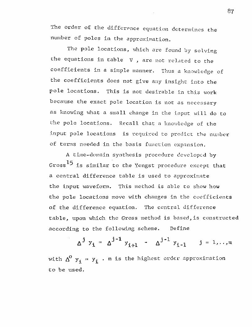
The order of the differPnce equation determines the
nwuber of poles in the approximation.
The pole locations, 't·Jhich are found by solving
the equations in table V , are not related to the
coefficients in a simple manner. Thus a knowledge of
the coefficients does not give any insight into the
pole locations. This is not desirable in this work
because the exact pole location is not as necessary
as knowing what a small change in the input will do to
the pole locations. Recall that a knowledge of the
input pole locations is required to predict the nwnber
of terms needed in the basis function expansion.
A ·time-domain synthesis procedure develope-d by
Gross 15 is similar to the Yengst procedure except that
a central difference table is used to approximate
the input waveform. This method is able to show how
the pole locations move with changes in the coefficients
of the difference equation. The central difference
table, upon which the Gross method is based,is constructed
according to the following scheme. Define
j = l, .. ,m
with 1)0 y. == y .. m is the highest ordt.r approximation 1. 1.
to be used.

88
The wavefo~~ is then approximated as
Where the a's are constants which are determined by
the mean-square error criterion. The normal equations
are shown in figure 6. 3
Since Y*(S) is to be a rational function of S,
y*(t) must be written as
= (6.19)
where xk is the root location. The difference table
was used to approximate sucessive derivatives of y*(t).
6j y. ------1...... (2Llt)j
Substituting 6.19 into 6.20 gives
Llj yi
• ( 6. 20)
This equation can be solved for Llj yi which is then
put into the original approximation, Yl . Replacing
m -v [ xkt. l.J K"!r a 1 ~e ~ + ... ·
k=l <'-

r ~: ( AY· )2 . ~
' I tt.2Yi.AYi
f •
•
•
'f,/lmy. AY· . ~ ~ j
all ~t.Yi A2Yi m
2: ~yi b. yi ' I 1
~ ( A 2Y. )2 Ll ~
i tt/Yi AmYi II a21
•
I I 1= •
a I }: ( 4 myi )2 •••••••• mj . t
FIGURE 6.3
Normal Equations in the Gross Method
r-
~ yi !l1i I
LYi ~2yi ' .. J
I. m l!Y· A Y· . ~ ~
f
OJ \0

90
Forcing equivalence on a term by term basis gives a set
of equations which is equivalent to finding the m roots
of the pol~1omial equation
+ a zm m . (6.21)
Although equation 6.21 can be solved directly using the
computer to locate the poles of Y*(S) , a usefull
approach is to solve this equation by the use of root
locus techniques~6 Then changes in the coefficients
can be related to changes in the pole locations. Thus
if a pole starts to move close to a preselected error
boundary, it is possible to detect which coefficients
are causing this movement and thus the parameter of
the input ~1aveform which is causing that particular
pole to move can perhaps be isolated. This will allow
the determination of what cor..stitutes the worst case
input to the signal.
As in the Yengst method, the choice of .6 t was
somewhat arbitrary. Gross found that the following
rules gave good results:
(1) Not more than one extremal of y(t) should occur
in the interval 2L\t.
(2) The funstion should not change more than about
20 °/0 of its maximum value in the interval 2 ~t.

These t\·JO restirction.s give some idea of the minimum
sampling required of the input waveform although too
many samples wi 11 cause nmnerical troubles as pointed
out earlier in the Yengst work. The order of the
difference equation is not discussed in Gross's work
either. Time domain synthesis techniques~ although
giving the locaticn of the poles of the i~put, present
tv·Jo additional problems. How many samples should be
taken of the input \·:aveform and -what order equation
should be fitted to the ~Javeform.
The reason for the numerical troubles can be seen
if the following form is used to write the central
difference approximation used by Gross. Let
and w(t.) = l,all i. ~
The normal equations in equation 6.16 become
n ro • L [Y·- 2: a.lJ? ll.J Yi] . 1 ~ .
~== J =0
k ll Y· ~ = 0
k = 0, 1, ... m
I11terch .. 1nging s unnua t ions gives
m [ .£ J.lj ll.k n
m Yi] r Y· l: a. Y· =
J ~ . 1 ~ j=o ~=1 ~=
Using the notation
n
ll.k Yi
91
ll.j k gjk = L y. fl. y.
~ ~ ( 6. 22)
i=l

and
= n r
i=l y. ~
k ll y. ~ .
The normal equations may be written
m
92
r gJ.k j=o
m a.
J k=O,l,2, • • • • m ( 6. 23)
If n i.s large, equation 6.22 becomes
k ll y i dt • ( 6. 24)
Equation 6.20 , in which the differences were used to
approximate the deri·vatives, can be substituted into
equation 6.24 ,giving
=
k d y. ~ dt .
This expression for the elements of the nonnal equation
matrix fu_ dependent on the derivatives of the function.
If the derivatives of the input are not restricted, ie.
the function is sampled too often,corresponding to a
large value of n, the matrix may become ill-conditioned
and require a large number of significant digits to
obtain the required accuracy's. If the input is
polynomial in nature, the ill-conditioning problem
of the normal equations will not be predominant as an
(m-l)st order polynomial has only m derivatives.
makes a statement to this effect in his work.
Yengst

93
" The pole positions determined by this procedure (Yengst)
are only best in the sense of least squares if the function
to be approxitnated satisifies an mth order difference
equation."
2. Polynomial Approximation of Input
Ralston,in his book on numerical analysis 17, shows
that a polynomial approximation with non-orthogonal
basis functions will give rise to ill conditioned
normal equation matrices. Thus fitting the input data
wi1:h a set of orthogonal polynomials before taking the
divided differences will eliminate many of the errors
which arise in this type of non-orthogonal expansion
of the input.
A question left unanswered in the time domain
synthesis procedures is the selection of the difference
equation which will fit the data. Using the fact that
a (m-l)st order polynomial can be fitted exactly by
a mth order difference equation reduces the above question
to finding the correct order of the approximating
polynomial. There are two characteristics required
of this approximation:
(1) It must be of sufficiently high degree so that
the approximating polynomial provides a good approximation
to the true function.
(2) It must not be of such a high degree that it fits
the observed data too closely in the sense that noise
or inaccuracies in the data are fitted.

Since a polynomial of order (n-1) can be fitted
through n poi.nts, a basic hypothesis that the input is
a polynomial will be assumed. Letting m = n-1 makes
n "' w. R~ i~l 1. 1.
equal to zero. Howeve~ in chasing this large value
of m , all smoothing properties of the least square
error fit are lost. Based on the assumption that the
errors in R. are normally distributed with zero mean 1.
94
and variance u- 2 /w. 1.
allows the use of the Null Hypothesis
described by Ralston. rt1e results of this test are
based on calculating the following quantity.
g2 m =
82 m
(n-1-m)
is computed for each m and m increased until no signifi
cant decrease occurs in v 2 • This gives the value of m m
which is the desired least-squares approximation satisif-
ying the Null Hypothesis.
To approximate the input function over the discreet
input data points, the Gram Polynomials17 will be used.
By definition, a set of polynomials { pj (x)} is
orthogonal over a set of points { ti} with respect to
a weight function wi if
n r
i=l w.
1. = 0 jlk

95
This proper-ty makes all non-diagonal terms equal to
zero in the noroal equations. ~.J"ith an odd number of
points used and n = 2L , a new variable s i~ defined as
s = i - L i = 0,1,2, . . . . n
The Gram polynomials are then defined as
pj ( s, 2L) = j "' sk e. L A jk
J k=o A . . = 1 .
]]
All .A jk 1 s not shown are zero. The coefficients in
this equation are given in table VI. The least-
squares approximation using the Gram polyno~ials is
then written as
where
y*(s)
b. = J
= m }.:
j=o b. p. ( s, 2L)
] ]
p~ ( s, 2L)] ] .
To convert these results into terms of t, it is only
necessary to make the change of variables
s = - L .
An additional advantage of using the Gram polynomials
to approximate the data is that noise is inherently
smoothed outo The divided differences are basically
derivatives and small errors in the input propagate
throughout the entire set of normal equations.
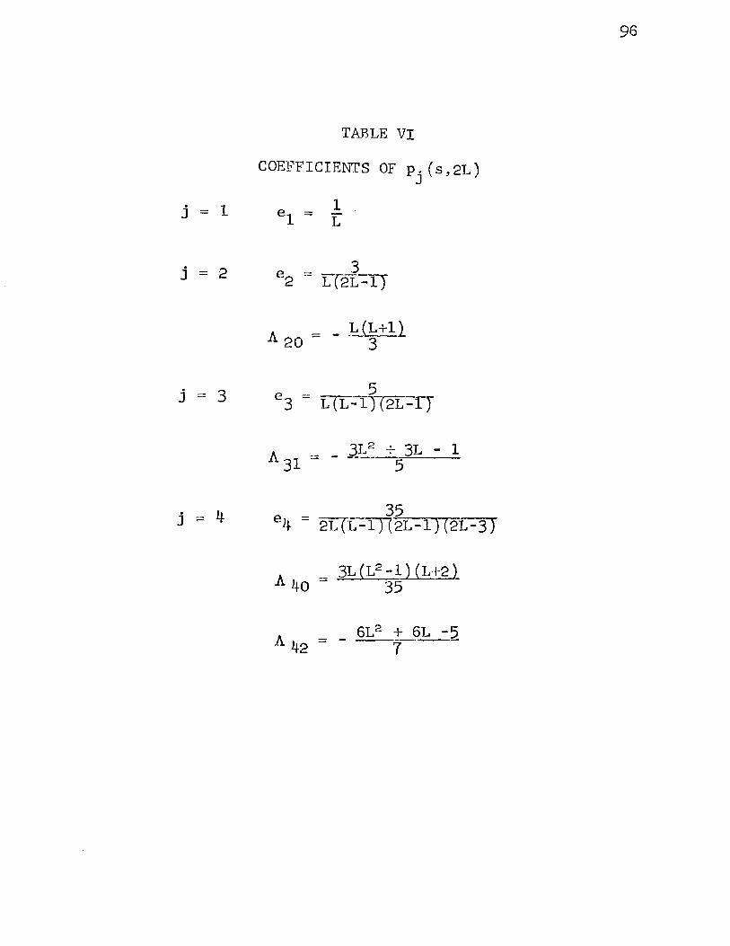
j = 1
j = 2
j = 3
j = 4
TARLE VI
COEFFICIENTS OF pj (s,2L)
1 e1 = L
3L2 + 3L - 1 A 31 = - ---- 5
35 e 4 = 2LTL~--=-l..,._,) ( 2L -1) ( 2L-3)
3L ( L 2 -1 ) ( L+2 ) A 40 = 35
6L2 + 6L -5 A 42 = - 7-·
96

97
This procedure, of approximating the input signal
with the Gram polynomials to determine the order of the
approximating polynomial, was applied to the -vmveform
shown in figure 1.2 . If the Gram polynomials were
used to approximate the waveform over the entire Interval
of zero to 1 second , the small ripples located at t ~ .7
seconds would be smoothed out. Thus these ripples would
be lost unless the order of the approximating polynomial
was large. As a result, only the interval from t = .6
to t :::::; . 9 seconds was approximated. For convenience_.
the time scale was shifted as shown in the sketch below.
0 .1 .2 time
The Gram polynomial approximation was performed
on a digital computer and the values for sigma squared
are shown,along with the coefficients in the Gram
1 · as a function of m in table VII. polynomia expansLon,
From this table, the null hypothesis suggests that
the value of the approximating polynomial of the input
should be a fourth order polynomial.

98
TABLE VII
o-2 AND b. Vs. J
j
j o-2 b.
0 ------ 0.409
1 0.0149 -0.349
2 0.0073 -0.170
3 0.0063 0.071
4 0.0051 0.069
5 0.0049 -0.035

99
This fourth order Gram polynomial approximation 'l.v~ls used
as the source of input data points for the Gross time-
domain synthes;s proced t 1 f 1 ~ - u~e -o so ve · or the a s of
equation 6. 21 . These coefficients were then substituited
into equation 6.21 giving
17.12 Z4 - 3-93 Z3 + 1.66 Z2 - 4.37 z- 1- o.
This can be rewritten as
l . 255 ( z + . 219 )
-- 0 Z2 ( Z2 - • 23z + . 097 )
The solution of this is equivalent to finding the poles
of a closed-loop system with gain = -.255 and with a
open-loop transfer -function
( z + . 219 )
Z2 ( Z2 - .232 + .097 )
The root locus plot of this system is shmvn in figure 6. 4.
The pole in the right-hand plane on the real axis is
due to the very oscillatory nature of the v1aveform
considered. The movement of the complex poles is shown
as a function of the gain. The gain in this case is
the ratio of the coefficient of Z to the coefficient
of Z4 • If several typical waveforms had been available I
it would have been possible to compute the a s for each
of these wavefonns and thus observe 'l.vbe·.ce the poles
were moving as the gain changed.
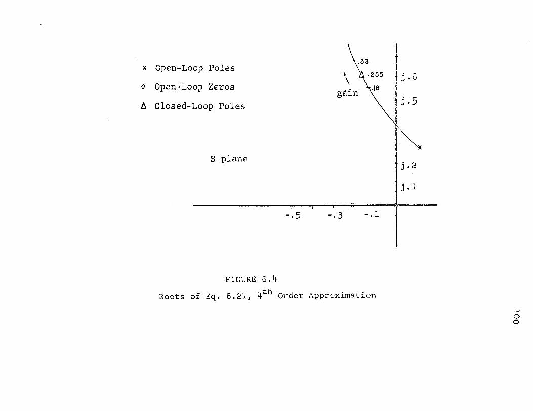
x Open-Loop Poles
o Open-Loop Zeros \ gain
.255
~ Closed-Loop Poles
S plane
-.5 -.3 -.1
FIGu~ 6.4
Roots of Eq. 6.21, 4th Order Approximation
I
L.s i t j. 5
j.2
j.l
....... 0 0

101
These changes in the coefficients must be small to avoid
a serious change in the open-loop polEs which would, of
course, have an effect on the root locus. The root
locations Zk are related to the pole locations of the
input function by the following constant
xk = zk I 2 ll t •
ll t in this problem was selected to be . 0125 seconds.
The dominant poles of the input are then located at
xk = 4o ( -. 16 ± j . 61 ) .
In the initial studies by the author, the input
waveform shown in figure 1.2 was empirically found to
be adequately represented by sampling every .1 seconds
and using six filters or terms in the expansion. The
reconstruction was found to have a maximum error of . 083
which corresponds to an "'] ~ • 01 • The effect of s.:unpling
every ol seconds is to reduce the frequency components
by a factor of ten. Thus the dominant pole positions
become
wh~ch d" from the origin of the S 4 corresponds to a ra LUS
plane of 2.5 •

102
Figure 6. 2 shows that it would require about 7 terms to
reduce'- to .05 . This suggests that the system is
overestimating the error by a factor of five. HovJever
the expression for the error is independent of phase
and the empirical reconstructions cited earlier vJere not
checked to see if some other phase would give a larger
error. Thus it is possbile that the error predicted
by this method is not as conservative as this exaraple
suggestso
As a matter of interest, the fourth-order Gram
polyDorJial approxiuation was used as the input for
a third-order pole approximation. Repeat:Lng the
same steps as for the fourth-order approximation gives
equation 6.21 as
10.7 Z3 + 3-9Z2 + 4.72 + 1 = 0
which can be rewritten as
1 + .44 ( z + 0 213 )
z2 ( z + .366 ) == o.o •
This corresponds to a closed-loop system with gain
and open-loop transfer function
( z + .213 )
z2 ( z + .366 )
= .44
The closed-loop poles are shown in the root locus plot
of figure 6.5 •

x Open-Loop Poles
o Open·Loop Zeros
~ Closed-Loop Poles
j.4
j.3
S plane j.2
j.l
... "
-.5 -.3 -.·1~1
FIGL~ 6.5
Roots of Eq. 6.21, 3rd Order A?rroximation
.._. 0 w

Sampling the input waveform again every .1 seconds
yields the poles of the input 'vaveforrn at
x, = - • 3 ± j 2 • 5 ~<
which is approximately the same location as in the
fourth order approximation of the poles.
104

CHAPTER VII
PROBLEMS FOR FURTHER STUDY
A Graphical Test Functions
105
The test functions described in chapter five wl:l·e:
easy to use in the determination of sarupling ratl: .:11".G
number of filters to be used, but they gave conscrv;_e; t i vc
error estimates. The following examples may be usc<.l
to generate some conditions which will make the tcs t
function approach more useful. Let the input f~nction
be defined as
f 1 (x) = 1 - x2 -l~x~l .
This input will now be bounded by ti.12 second test
fUJ.J.ction which is a tria.ngle o£ base two and heigh.t
F • F will be determined by evaluating the slope
of the function at the start of the interval.
i
F = f~ (x) I = 2 .1. x=-1
The following sketch shows this input and the test
function bounding it.
Function

106
The maximum value of the input function is at x = 0.
The The maximum value of the test function is F.
third coeffieient in the Legendre polynomial expansion
of the input is bounded by
actually computed to be
c -2 -
Observe the following ratios.,
F nor = 2
C2 (mclX) ----- --
c2
.689 F
.666
= .666
= 1.03 F = 2.06
This indicates that the ratio of F to the maximwn value
of the input function is indicatitive of the ratio of
the bound on the coefficient to the actual coefficient.
This input function only requires three terms to be
exactly represented with a Legendre polynomial expansion.
Consider now a function with an infinite number of terms
in its power series expansion. Let the input function
be given as
TTX = cos 2 -1 ~X~ 1
The maximum value of this function also occurs at
x = 0 and has the value of one.

' F == f 2 (x) 1
X==-1
The third coefficient in the expansion is given as
5 Jl 7TX Ij:' cos 2-
-1 -7
Now the coefficient is bounded by c2 (max) ~.689 F.
Computing the same ratios again gives
F £To)
=
7f
2 == 1. 5'7
. 689 F
·7 = 1. 54.
Or again the conservative nature of the coefficient
is indicated by the ratio of the maximum of the test
function to the maximum of the input function.
Both of these inputs were symmetrical about the
origin and had their maximum derivatives at the start
107
of thr2 interva 1. This determined the maximum slope of
the test function and thus the heigth F of the test
function. This Qethod of finding F fails if the input
contains a derivative which is not bounded at the start
of the interval. Consider the following input which
is sketched below. It has an infinite derivative at
the start of the interval.

108
- 00
-1 0 -+1-x
A method to circumvent this is shown in this sketch.
F
A X
Now it is necessary to know what the input is doing in
the interval betwee_n points A and -1 and bet\·:·ecn 1 and B.
If the input is monotonically increasing or decreAsing
and has a nonzero derivative throughout these two intervals,
the conditions of the original test function ( covering
the interval A to B ) will not have been violated.
However,.,even if the function is changing in the two
small intervals, it is possible to construct a 'tent'
function to use for bounding the input.
F

Hith the use of this tent function, it is possible to
obtain a close fit to the input even though the input
may contain a large derivative at the start of t1lc- intt rv:11.
An investigation of the conservative n.:1turc of the
coefficients might yield some interesting results and
with additional study, the tent function appro:1ch ::1.1y
produce a better way to graphically classify the input
signalso
B Derivative Approximation
In chapter 3, the derivative approximation of
the input signal was discussed. This method \·:as ,:( '-'' lt P( d
to avoid the problem of discontinuities at tht.: 5 •1·-:;plc
points. Since each interval of approximation is
· d · 1.'nte.~.vals, it is poss~blc ln ependent of the prev1.ous
no t be continous fro;n int c n::sl that the approximation will -
to inte1.-val 0
the derivative of the In approximating
l.·s obtained by integrating input, the final approximation
the derivative
approximation.
. ld'ng a co~tinuous approximation y1.e 1. '
Shows the result of this Figure 7ol
When the values of the system continuous integration
The input ~avcfonn were improperly choseno ( a==· 05 )
is shown in Figure 1. 2

110
15,------· r--- ------T -------- --,-------~ 1---- ----~---·--· -·-· ··- - - .. . - - (\ - .
. -----r---~--- ~-~~-- ----------- ------- ----r ... ~- ----·--·- ·-----------·-- -------· ---- - I
1- ....... I .. . ·--· ... - il - \- - - I --~----i ~---·------+------,-----1-- ___ _t ___ --------- ---~ I l ~--- _____ 1 ___ , ____ 1 J'~ r·-J·--·--,-- -- ~
I 1 -------- . -- ..... . -· - · v1 · ',J--10. , --+------~-~ -- f ! I'~ I r .. -,- ····1-/ .. --~-~ -=--- ~--,, = ~-- --- -· -v
-,---------··-t--------···· --f-T ______ -------- ---- I --- ··-~----.. .. - . 1- + ---- ---- -- - l .
, I I ------- ----- ---r,J--- ------ ----- --- -- ----- ______ t-' _
..... - -. I I ---- - ------ -- ·- -· -----1 · -- · · -· · r ·- ------ ··· ·· ··-- - -·----- -- · I ~ --------- ---------· rl-------- ------- ----- -- ----- ·---+---+------
. I _, ~--0--- ·······!- - -----·----.--- ---' __ L ___ j ___ , __ j_____ , ____ _l __ l_ s..______.J
LJ • I Li • l c: , 3 li , I Li. 5 S , ,; 0 • 7 ·' • <3 ·,:,. ;,
Time (sec.)
FIGURE 7.1
Reconstruction Sho"t-ling the Accumulation of Error

111
This figure shows how the error in each interval
2ecumulates causing the final intervals to be in gross
error. Recall that to form the derivative approximation~
it '!;·Jas necessary to obtain a sample of the input \·mveform
at the end of each interval. Thus, it is possible to
check the reconstructioncby the basis functions against
che sampled values of the function. Figure 7.2 shows
~ plot of the error at the sample points. These error
points were connected by a straight line and this signal
\vas subtracted from the approximation shown in figure
7 .1. This yielded i.:he approximation showl.1 in figure 7. 3 .
This is not a bad reconstruction considering the poor
choice of alpha. The interesting thing about this
reconstruction is that a straight line was connected
bet·\\.1een the error points in figure 7. 2. Since this is
a exponential basis function reconstruction and the
weighting function is exponential in nature~ it seems
J1at the function which should be drawn between these
error points should be exponential in nature.
C Error Analysis
The error analysis presented in chapter 6 gave an
expression for the m<1xi.mum relative error which could
occur as a function of the pa.rameters N and T0 • The basis
function expansions are designed to minimize the mean
squar,-_ error of the approximations.

112
-~---~---·r----r---..,----o[~-·
---- ----- --------- --- - ---- ----- I -----
5----
-- ------ -- -- -· ------ ------------- -f- -·-----·-
6 ·-------·- --
~- -- r J ------ ---- -----·-- ----r----
Ll • :
---------- -- ---
L.l. i! ll. J L),4
0.~ u.6
Time (sec.)
FIGURE 7.2
- - ~
-----+----·-- -----
c. 7 j. 8 . '. j
Plot of Error at sample Points of Fig. 7.1
-

113
r---.-----r\l-----sr------4-------L------++~r---t-------~--------~------ --------~-----4------~
~------1-------:------ 1------ r--------1-------- -----_-- --------:--------- --------
6~---- ------~---·---u-------tt, -~---t--+---t--_j ___ ..,.
----·-- ------- e-------i------1~-~-------+- ----- ----
4 .. _____ -:___ ------ ---l-----------+v-J.\..~.,-L-------+------1----~-----I------ j I
f--·-----------f------------- -----+--+--------~- i I --~---·---+----1---------- -------t--------, I"' - i
.~_-----------+--r---------- ~----+--/-4-----i---+-1 \J\ L_ !
Gf------~~~ .. ~~~-~~-~~+·~~--~------~~-----
~-------1-----~~---- ·-----~-----+---+-----+----l---~ -z ---~·
----G 0.1 o.z o.~ :).4 0.5 0.6 0.7 Q.l 0.9
Time (sec. )
FIGURE rr. 3
Reconstruction wi.th Zero Error at the sample Points

114
It would be interesting if the results of chapter 6
could be extended to give the MSE of the approximation.
Useful ratios of MSE to MSV would probably require
fewerfilters than are now specified. The trouble
with expressions involving the MSE is that if there is
a discontinuity in the signal, the magnitude of the
mean- square error will not show that a crude approxir.1.:1 tion
·Nas obtained at the discontinuity. HovJever, this is not
of much impo1.·tance for the signals \vhich \vould be
considered as inputs to this kind of a system.
Concerning the error, another interesting study
would be to input noise to the pole-locator techniques
and calculate where the poles of the signal plus noise
are located. Since the pole locator sche~es depend upon
calculating the derivatives of the input, the error in
the pole locations should increase rapidly as the signa~
to-noise ratio decreased. Then input the signal plus
noise into the pol)~omial approximation scheme. The
polynomial approximation should smooth out the noise.
This polynomial approximation would then be used as input
data for the pole locator schemes and the pole positions
calculated a It would be of intecest to see how much
improvement was obtained by approKimating the input
with a polynomial first.

115
D Bandlimited Signals
The signal theory system is sensitive to time-domain
inputs since the reconstruction is '\.Yith basis functions
orthogonal in time. Techniques to apply bandlirnited
signals as a class into this system have not been developed.
In most cases~ the signal to be sampled will be prefiltered
to remove all high frequency components and noise which
are not of interest. In this case~ an interesting
approach is available.
The general input signal to be represented can be
approximated with a series of short,straight line segments.
The first derivative of the straight line approximation
will yield a series of step functions~ and the second
derivative will yield a series of impulses. If this
train of impulses is applied to the input of the pre
filter~ the output is a summation of the impulse responses
of the filter~ each impulse response starting at a later
instant in time. The actual prefiltered signal is the
second integral of the impulse response outputs.
G(S) Vout(S) = S2 .. .
Where G(S) is the transfer function of the prefilter.
The impulse response is due to the poles of G(S) and
these will be knowno Thus, if the sighnl theory system
can represent the impulse response of the filter~ it
can represent any signal which is prefiltered by this
filter.

116
The two additional poles at the origin of the s plane
contribute nothing in the error · d 1 express~ons eve oped
in chapter 6. Figure 7.4 shows a general input
approximated with straight line segments and the first
two derivatives. The second derivative can be expressed
as
and thus
m f"(t) = 2:
k=o
the output
-a S e k
of the prefilter
G(S) -a S m e k vout(t) 2: = •
k=o s2
is given as
The problem to be solved here is that the output is the
st~mation of the impulse responses. Each one of the
impulse representations will have some error asscoiated
with it and thus the error in the total representation
of the signal is not bounded in general.
The use of general bandlimited signals is of interest
as this is anengineering method currently used for
classifying signals.
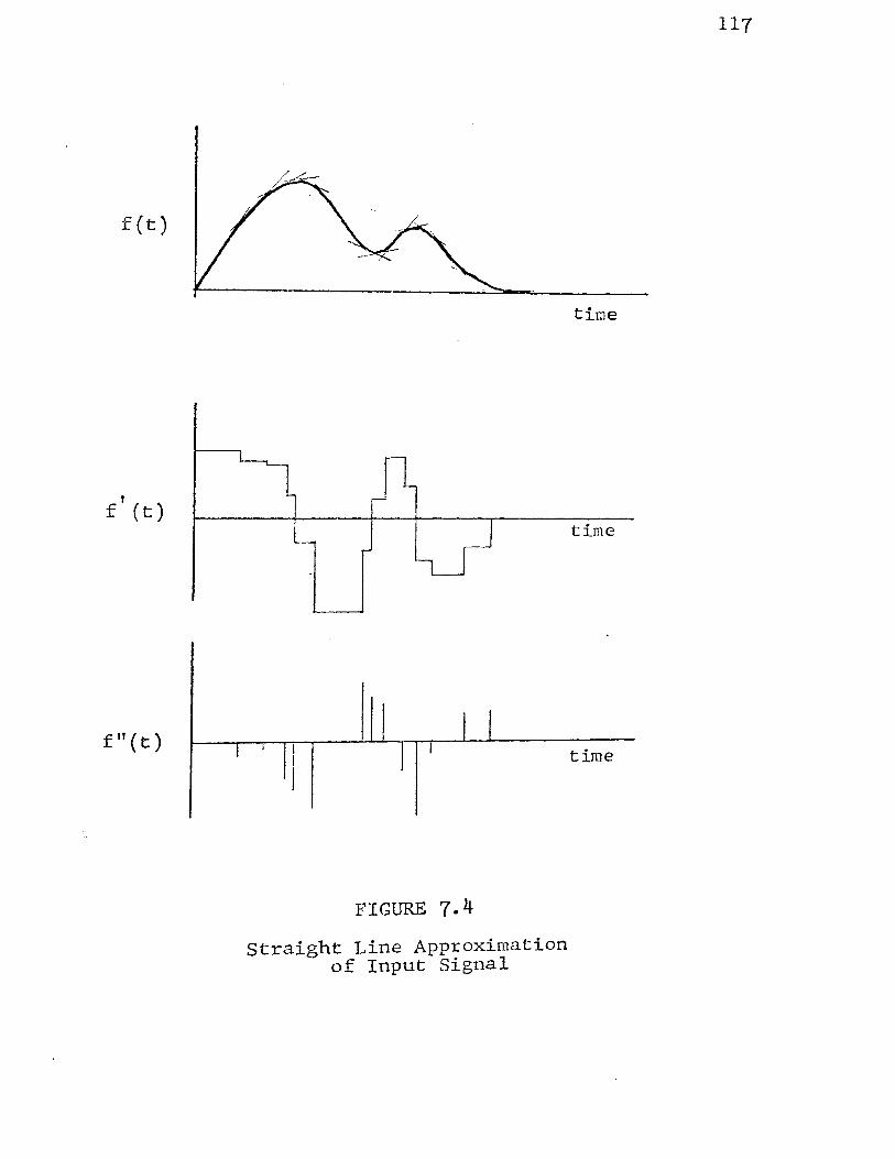
f(t)
' f (t)
f"(t)
FIGURE 7.4
Straight Line Approximation of Input Signal
117
time
time
time

1.
BIBLIOGRAPHY
W. H. Huggins, " The Use of Ortho3onalized
Exponentials," Report AFCRC TR- 57- 357,
AD 133 741, November 1958.
118
T. Y. Young and rv. H. Huggins, II 'Ccmplementary'
Signals and Orthogonalized Exponentials," IRE
T~ans. on Circuit Theory, Vol. CT-9, No. 4,
pp. 362-370, December 1962.
3. W. H. Kautz, " Transient Synthesis in the Time
Domain," IRE Trans. on Circuit Theory, Vol. CT-1,
pp. 29-39, Sept. 1954.
4. I. M. Horowitz, Synthesis of Feedback Systems.
New York: Academic Press, 1963, pp. 680-682 .
5. D. c. Ross, "Orthonormal Exponentials," IEEE
Trans. on Communications and Electronics, Vol.
CE-1, pp. 173-176, March 1964.
6. J. M. Hendel, 11 A Unified Approach to the Synthesis
of Orthonormal Exponential Functions Useful in
Systems Analysis," IEEE Trans. on Systems Science
and Cybernetics, Vol. SSC-2, No. 1, PP· 54-62,
August 1966.
119
7 · T · Y. Young and W. H. Huggins, 11 On t~1e R<." pres en ta
tion of Electrocardiograms, 11 IEEE Trans. on
Bio-Medical Electronics, BME-10, No. 3, pp. 86-95,
July 1963.
8. H. M. Barnard and J. J. Baremore, 11 Signal Theoretic
Characterization of a Function using Orthogonal
Positive Exponential Basis Functions, 11 Hawaii
International Conference on Systems Science,
January 1968.
9. E. T. wbittaker and G. N. \-Jatson, A Course of
Modern Analysis, London: Cambridge Thtiversity
Press, 1920 ,. pp. 302-336.
10. J. G. Truxal, Control System Synthesis, Ne-;oJ York:
McGraw- Hill, 1955, pp. 203-212.
11. M. E. Van Valkenburg, Modern Network Synthesis,
New York: Wiley , 1962.
12. L. B. w. Jolley, Summation of Series, New York:
Dover, 1961, pp. 119, 157·
13. M. Abramowitz and I. A. Stegun, Handbook of
Mathematical Functions, VJashington, DC: U.S.
Government Printing Office, 1964 , PP· 798 ·

120
14. W. C. Yengst_, 11 Approximation to a Specified
Time Response_," IRE Trans. on Circuit Theory_,
Vol. Ct-9_, No. 2_, pp. 152-162_, June 1962.
15. C. A. Gross_, 11 A Hethod for Approximating a
Specified Impulsive Response_," M.S. Thesis,
Univ. of Hissouri at Rolla_, Rolla , Mo. , 1966.
16. J. G. Truxal_, Control Systems Synthesis_, Ne'\v York:
HcGraw - Hill, 1955_, pp. 221-270.
17. A. Ralston_, A First Course in Nwnerical Analysis,
New York: McGraw-Hill _, 1965_, pp. 228-317.

121
VITA
James Julius Baremore was born in St. LouisJ Missouri
on September 15, 194lo He graduated from Webster Groves
High School in St. Louis in June of 1959. The Bachelor
of Science Degree in Electrical Engineering was received
from the Missouri School of Mines and Metallurgy in May,
1963. From 1963 to 1965J the author was employed by
t:he S-3-ndia Corporation in AlbuquerqueJ New Mexicoo
Sandia Corporation sponsored a program where employees
would vJork a half day and carry a full time graduate
load at the University of New Mexico. The Master of
Science Degree in ~lectrical Engineering was received
there by the author in June 1965. The author entered the
Graduate School of the University of Missouri at Rolla
in September of 1965 and has been employ.ed as a half ...
time instructor in Electrical Engineering.
The author is a member of the following socities:
Sigma Xi, Phi Kappa Phi, Tau Beta Pi, Eta Kappa Nu.
He is married to the former Donna Benish of St. Louis
and they have one boy, Michael.