1

Signal Processing by Neural Networks

Aurelio Uncini

INFOCOM Dept.

University of Rome “La Sapienza”

e-mail: aurel@ieee.org

International Joint Conference on Neural Networks, Washington, DC USA, July 18 2001

2

Agenda

Neural architectures for real-time DSP Non-linear generalizations of FIR-IIR filters by Dynamic Multilayer Perceptron (DMLP) neural networks;Fast adaptive spline neural model for signal processing

Some Applications

2

3

linear DSP: it's enough ?

major classical DSP techniques are based on linear models

in the real world the processes are non-linear

linear structures could not be able to model them adequately

3

4

specific non-linear architectures

particular class of problemsefficient but specific

e.g.median and bilinear filterssome spectral analysis techniques…

generic non-linear architectures

large class of problemgeneral but complex

e.g.Volterra filtersnon-linear state equationspolynomial filtersfunctional links…

non-linear DSP: classical approaches

4

specific or generic?

5

non-linear DSP: desired approaches

"standard" architecture with scalable complexity;

capability to approximate any non-linear (dynamic) behaviour;

"standard" design algorithms;

good implementation efficiency

use of the available know-how on linear filters;use of the available DSP processors for real-time audio applications.

5

generic and efficient

6

non-linear DSP: a different approach

dynamic = capability of processing temporal sequences

⌧how to get dynamic behaviours from an ANN;⌧non-linear FIR/IIR architectures;⌧design methods or learning process.

6

Dynamic Artificial Neural Networks (discrete time ANN)

7

ANN: Multi-Layer model

sgm

sgm

sgm

x

x

1

2

Nw1N

y2

.

.

.

x

+x

x

1

2

N w N

x1w

w2

s

sgmy

.

.

.

sgm

sgm

.

.

.

.

.

.

w2M

w11 21w y

1

My

(b)

(a)

”Artificial neurons" arranged in layers Multi-Layer Perceptron (MLP)

feedforward structure without delaysno dynamics

approximation of any non-linearityCibenko ‘88, Hornik et al. ‘89non-linear universal approximator

sgm

7

8

Dynamic Multilayer Networks (DMLP)

External memorythe non-linear filter is built using a static MLP inside a FIR/IIR framework

external delay lines ("buffers")Narendra-Partharasarathy 1990

Internal memorythe non-linear filter is built using a MLP with neurons containing FIR/IIR filters

internal delay lines ("dynamic neuron")Waibel et al. 1989, Back-Tsoi1991/94, Frasconi et al. 1992, Campolucci et al. 1999, etc.

Delay lines (memory elements) put dynamic in the multilayer model

8

9

DMLP with external memory FIR scheme

allows to use the classical multilayer model;

straightforward generalization of the linear FIR filters: linear filter ≡ DMLP with one neuron + (f(.) = identity)

x[k]

x[k-1]

x[k-M+1]

y[k]Output

Signal

MLP

z -1

Input Signal

z -1

z -1

9Universal Functional Approximator

10

DMLP with external memory IIR scheme

allows to use the classical multilayer model;

straightforward generalization of the linear IIR filters: linear filter ≡ DMLP with one neuron + f(.) = identity

y[k]OutputSignal

MLP

z -1

z -1

x[k]

x[k-1]

y[k-1]

y[k-2]

Input Signal

z -1

z -1

z -1

feedback

11

DMLP with internal memory

several different research contributions (already object of studies);

another generalization of the linear FIR/IIR filters: linear filter ≡ DMLP with one neuron + (f(.)=identity)

multilayer network composed by "dynamic" neurons

y[k]

Input Signals

OutputSignal

MLPD

D

D

D

D

D

D

D

D = dynamic neuron

11

12

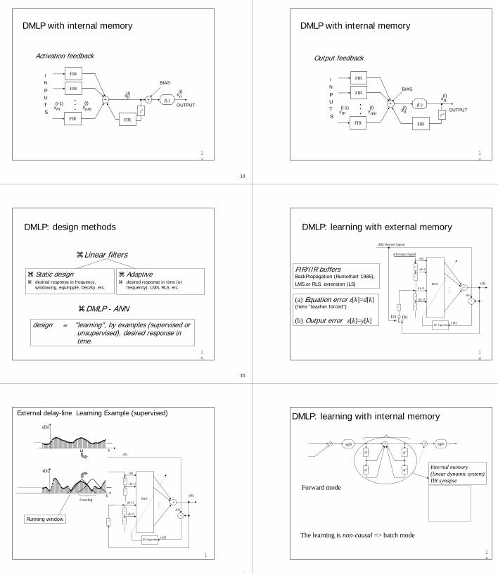
DMLP with internal memory

FIR/IIR synapses

... OUTPUT

BIAS

I

N

P UTS

x(l)

s(l)n

n

y(l)nmx

(l-1)m

f(.)

FIR/IIR

FIR/IIR

FIR/IIR

12

13

DMLP with internal memory

Activation feedback

...

BIASIN

P UTS

s(l)n

y(l)nmx

(l-1)m

FIR

FIR

FIR

OUTPUT

x(l)nf(.)

Z-1

FIR

13

14

DMLP with internal memory

Output feedback

...

BIAS

IN

P UTS

s(l)ny(l)nmx

(l-1)m

FIR

FIR

FIR

OUTPUT

x(l)nf(.)

Z-1

FIR

14

15

DMLP: design methods

Static designdesired response in frequency, windowing, equiripple, Deczky, etc.

Adaptivedesired response in time (or frequency), LMS, RLS, etc.

Linear filters

design ≡ "learning", by examples (supervised or unsupervised), desired response intime.

DMLP - ANN

15

16

DMLP: learning with external memory

z-1

z-1

z-1

z-1

x[k] Input Signalx[k]

x[k-1]

•••

MLPz[k-1]

z[k-2]

y[k]

(a) (b)

z-1

BP Algorithm

d[k]

ε [k]

FIR/IIR buffersBackPropagation (Rumelhart 1986), LMS or RLS extension (LS)

(a) Equation error z[k]=d[k](here "teacher forced")

(b) Output error z[k]=y[k]

d[k] Desired Signal

16

17

External delay-line Learning Example (supervised)

1

x[k]

k

d[k]

k

z-1

z-1

z-1

z-1

x[k]

x[k-1]

•••

MLPz[k-1]

z[k-2]

y[k]

z-1

BP Algorithm

d[k]

ε [k]

d[k]

Overlap

Running window

18

18

sgm(2)1 [ ]x t(2)

11(0)w

(2)11(2)v

(0)1 [ ]x t

(0)2 [ ]x t

(1)1 [ ]x t

1

1

( , ) 1 ( , )

B t qA t q

−

−−

(2)11(1)w

(2)11(2)w

(2)11(1)v

sgm(1)11w

(1)12w

(1)1 [ ]s t (2)

11 [ ]y t

DMLP: learning with internal memory

( )

1

1( ) ( ) ( 1) ( ) ( 1)

( ) ( )0 1

( ) ( )

0

( ) ( )

[ ] [ ] [ ];

[ ] [ ];

[ ] sgm [ ] ;

l lnm nm

l

L Il l l l l

nm nm p m nm p nmp p

Nl l

n nmm

l ln n

y t w x t p v y t p

s t y t

x t s t

−

−− −

= =

=

= − + −

=

=

∑ ∑

∑

Forward mode 1

1

11

1

11

( , ) [ ] ( )1 ( , )

( , ) [ ]

( , ) [ ]

Np

pp

Mp

pp o

B t qy t x tA t q

A t q v t q

B t q w t q

−

−

−− −

=

−− −

=

⎛ ⎞= ⎜ ⎟−⎝ ⎠

=

=

∑

∑

Internal memory (linear dynamic system)IIR synapse

The learning is non-causal => batch mode ( )2( )

1[ ] [ ] ;

TM

n nt

J d t x t=

= −∑

q-1

q-1

q-1

q-1

(1)2 [ ]s t

19

19

sgm

sgm’

1

1

( , ) 1 ( , )

B t qA t q

+

+−

(1)11 [ 1]w t∆ +

sgm’

1

1 1 ( , )A t q−−

(2)11(1)[ 1]v t∆ +

(2)11(2)[ 1]v t∆ +

-

d[t]

(2)1 [ ]x t

(2)11(0)w

(2)11(2)v

(0)1 [ ]x t

(0)2 [ ]x t

(1)1 [ ]x t

1

1

( , ) 1 ( , )

B t qA t q

−

−−

µ

(2)11(1)w

(2)11(2)w

(2)11(1)v

sgm(1)11w

(1)12w

(2)11(0)[ 1]w t∆ +

(2)11(1)[ 1]w t∆ +

µ

q-1

q-1

q-1

q-1

(1)1 [ ]s t (2)

11 [ ]y t

(1)12 [ 1]w t∆ +

RBP: General framework to derive several causalisedon-line approximations learning algorithms for DMLP

DMLP: Recursive Backpropagation (RBP)

(2)11(2)[ 1]w t∆ +

RBP signal flow graph

20

DMLP: complexity, implementation

Computational complexity(fast learning algorithms)

Structural complexity (in terms of number of interconnections)

A suitable activation function can increase the Neural Network representation property

Fewer neurons needed

• small structural complexity• small computational complexity 2

0

21

A New Neuron Architecture

Theoretical framework Extention of the Cybenko theorem : (Hornik, Stinchcombe, White, 1989)

neurons which present any "squashing" activation function maintain the universal approximation characteristics

GOALS FOR THE NEW NEURONA "more sophisticate" activation function;Retains the squashing property of the sigmoid;Necessary smoothing characteristic;Easy to implement both in hardware and in softwareFlexible (by the adaptation of few free parameters).

21

22

A New Neuron Architecture’s Activation Function

• Squashing characteristic

s

G

-G• Flexible shape

Two needed properties

New Neural Network Architecture with Flexible Adaptive Activation Function

22

23

Adaptive Spline Neural Network (ASNN)

x0 x1 xNxN-1xN-2xN-2x2 x3

i=0 i=1i=N-4 i=N-3

h(x)

Using Catmull-Rom or B-splines functions, with uniformly spaced control points, the shape of the activation function is controlled by few parameters (3rd degree: four control points).

x

Local shape adaptationSmooth characteristic: suitable for signal processing applications

2

24

ASNN: Spline Activation Function

iQ1iQ+

2iQ+ 3iQ+

0x

u x∆

x

( )h x( , )h u i

x∆

Catmull-Rom

B-Spline

Spline activation function is specified as the weighted average of the four equally spaced control points

( ) ( ),y h x h u i= =1 2 3, , ,i i i iQ Q Q Q+ + + 2

4

25

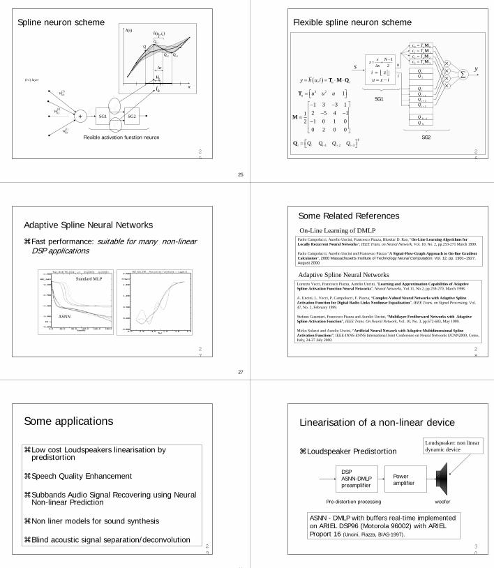
Spline neuron scheme

( 1)0lx −

( 1)1lx −

( 1)lix −

( 1)lNx −

( )0l

kw

( )1l

kw

( )lkNw

SG1 SG2

( )lks

( )lku

( )lki

( )lkx

(l-1) layer

+

Flexible activation function neuron

25

iQ1iQ+

2iQ+ 3iQ+

ku

x

( )h x( , )k kh u i

x∆

ik

26

Flexible spline neuron scheme

∑y

i

u ××××

iQ1iQ +

2iQ +

3iQ +

1Q

NQ1NQ −

s

0 0uc T= M1 1uc T= M

3 3uc T= M2 2uc T= M

2Qi z= ⎢ ⎥⎣ ⎦

12

x Nzx

−= +∆

u z i= −( ), u iy h u i= = ⋅ ⋅T M Q

3 2 1u u u u⎡ ⎤= ⎣ ⎦T

1 3 3 12 5 4 111 0 1 02

0 2 0 0

− −⎡ ⎤⎢ ⎥− −⎢ ⎥=−⎢ ⎥⎢ ⎥⎣ ⎦

M

1 2 3

T

i i i i iQ Q Q Q+ + +⎡ ⎤= ⎣ ⎦Q

SG1

SG2

26

27

Adaptive Spline Neural Networks

Fast performance: suitable for many non-linear DSP applications

27

Standard MLP

ASNN

28

Some Related References

28

Lorenzo Vecci, Francesco Piazza, Aurelio Uncini, "Learning and Approximation Capabilities of Adaptive Spline Activation Function Neural Networks", Neural Networks, Vol.11, No.2, pp 259-270, March 1998.

A. Uncini, L. Vecci, P. Campolucci, F. Piazza, “Complex-Valued Neural Networks with Adaptive Spline Activation Function for Digital Radio Links Nonlinear Equalization”, IEEE Trans. on Signal Processing, Vol. 47, No. 2, February 1999.

Stefano Guarnieri, Francesco Piazza and Aurelio Uncini, “Multilayer Feedforward Networks with Adaptive Spline Activation Function”, IEEE Trans. On Neural Network, Vol. 10, No. 3, pp.672-683, May 1999.

Mirko Solazzi and Aurelio Uncini, “Artificial Neural Network with Adaptive Multidimensional Spline Activation Functions”, IEEE-INNS-ENNS International Joint Conference on Neural Networks IJCNN2000, Como, Italy, 24-27 July 2000.

Paolo Campolucci, Aurelio Uncini, Francesco Piazza, Bhaskar D. Rao, "On-Line Learning Algorithms for Locally Recurrent Neural Networks", IEEE Trans. on Neural Network, Vol. 10, No. 2, pp.253-271 March 1999.

Paolo Campolucci, Aurelio Uncini and Francesco Piazza “A Signal-Flow-Graph Approach to On-line Gradient Calculation”, 2000 Massachusetts Institute of Technology Neural Computation, Vol. 12, pp. 1901–1927, August 2000.

On-Line Learning of DMLP

Adaptive Spline Neural Networks

29

Some applications

Low cost Loudspeakers linearisation by predistortion

Speech Quality Enhancement

Subbands Audio Signal Recovering using Neural Non-linear Prediction

Non liner models for sound synthesis

Blind acoustic signal separation/deconvolution29

30

Linearisation of a non-linear device

Loudspeaker Predistortion

ASNN - DMLP with buffers real-time implemented on ARIEL DSP96 (Motorola 96002) with ARIEL Proport 16 (Uncini, Piazza, BIAS-1997).

DSPASNN-DMLP preamplifier

woofer

Power amplifier

Pre-distortion processing

30

Loudspeaker: non linear dynamic device

31

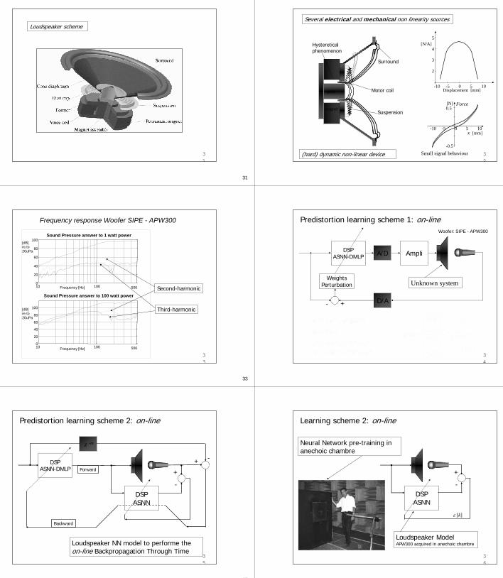
Loudspeaker scheme

31

32

Several electrical and mechanical non linearity sources

(hard) dynamic non-linear device

Displacement [mm]-10 -5 0 5 10

5

4

3

2

[N/A]l

dl∫B

32

Surround

Suspension

Motor coil

Hystereticalphenomenon

pole

magnet 0.5

-0.5

-10 -5 0 5 10

[N]

x [mm]

Force

Small signal behaviour

33

10 1000

20

40

60

80

100

Frequency [Hz]

[dB]re.to20uPa

Sound Pressure answer to 1 watt power

10 1000

20

40

60

80

100

Frequency [Hz]

[dB]re.to20uPa

Sound Pressure answer to 100 watt power

500

500

Second-harmonic

Third-harmonic

Frequency response Woofer SIPE - APW300

33

34

Predistortion learning scheme 1: on-line

DSPASNN-DMLP A/D Ampli

D/A

WeightsPerturbation

- +

( 1) ( ) ( ) ( )ˆˆ ˆ ˆ( )k k k kη+ = −w w g w

ˆ ( ) ( )J⋅ ≈ ∇ ⋅g

( ) ( ) ( ) ( ) ( )

( ) ( ) ( ) ( ) ( )

ˆ( )ˆ( )

k k k k k

k k k k k

z J c

z J c

ε

ε+ +

− −

= + ∆ +

= − ∆ +

w

w

( ) ( )

( ) ( )1( )1

1

( ) ( ) ( ) ( )1( ) ( ) ( )

( ) ( ) ( )

1( )( ) ( )

( ) ( )

2

ˆ ˆ( )2 2

2

k k

k kk

k k k kk k k

k k k jj

kk k n

k kn

z zc

z z z zc c

z zc

+ −

−

−+ − + −

−

+ −

⎡ ⎤−⎢ ⎥∆ ⎡ ⎤⎢ ⎥ ∆

⎢ ⎥⎢ ⎥⎢ ⎥⎢ ⎥

− − ⎢ ⎥⎢ ⎥= = ∆⎢ ⎥⎢ ⎥∆⎢ ⎥⎢ ⎥⎢ ⎥⎢ ⎥⎢ ⎥⎢ ⎥ ∆⎣ ⎦−⎢ ⎥

⎢ ⎥∆⎣ ⎦

g w

Woofer: SIPE - APW300

34

Unknown system

35

Predistortion learning scheme 2: on-line

DSPASNN

Loudspeaker NN model to performe the on-line Backpropagation Through Time

DSPASNN-DMLP

-+

z -m

Forward

Backward

-

+

35

36

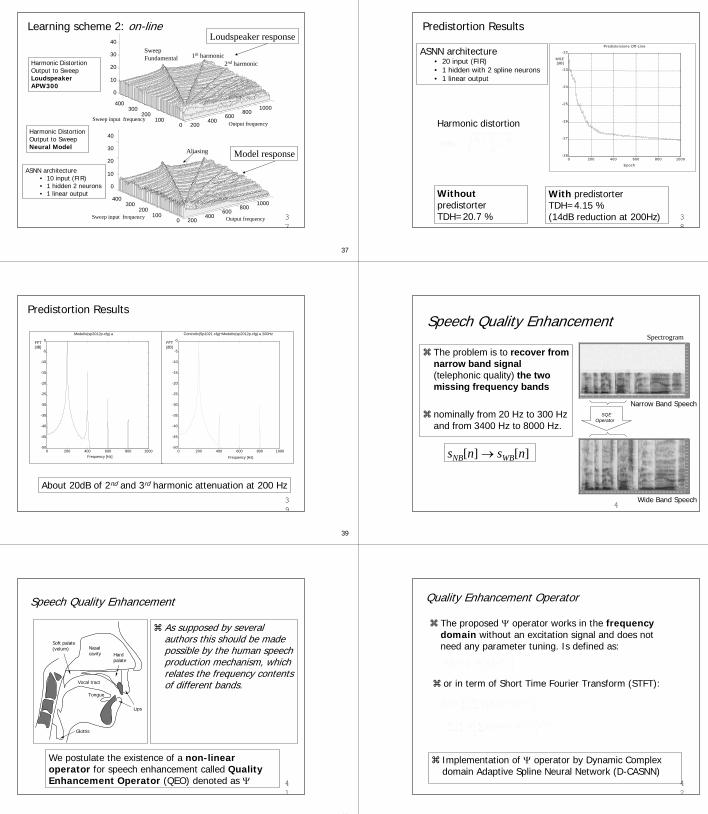
Learning scheme 2: on-line

Neural Network pre-training in anechoic chambre

DSPASNN

-

+

Loudspeaker ModelAPW300 acquired in anechoic chambre

36

ε [k]

37

Learning scheme 2: on-line

200400

600800

1000

0100

200300

400

0

10

20

30

40

Harmonic Distortion Output to Sweep Loudspeaker APW300

SweepFundamental 1th harmonic

2nd harmonic

Output frequencySweep input frequency

0

10

20

30

40

200400

600800

1000

0100

200300

400

Harmonic DistortionOutput to Sweep Neural Model Aliasing

ASNN architecture• 10 input (FIR)• 1 hidden 2 neurons• 1 linear output

Sweep input frequencyOutput frequency

37

Loudspeaker response

Model response

38

ASNN architecture• 20 input (FIR)• 1 hidden with 2 spline neurons• 1 linear output

Predistortion Results

2 2 2

IV 2II III IV

I

A A AA

+ +=THD

Harmonic distortion

0 200 400 600 800 1000-28

-27

-26

-25

-24

-23

-22

Epoch

MSE [dB]

Predistorsione Off-Line

WithoutpredistorterTDH=20.7 %

With predistorterTDH=4.15 % (14dB reduction at 200Hz) 3

8

39

About 20dB of 2nd and 3rd harmonic attenuation at 200 Hz

Predistortion Results

0 200 400 600 800 1000-50

-45

-40

-35

-30

-25

-20

-15

-10

-5

0

Frequency [Hz]

FFT[dB]

Modello(sp2012p.cfg) a

0 200 400 600 800 1000-50

-45

-40

-35

-30

-25

-20

-15

-10

-5

0

Frequency [Hz]

FFT[dB]

Controllo(Sp1021.cfg)+Modello(sp2012p.cfg) a 200Hz

39

40

Speech Quality Enhancement

The problem is to recover from narrow band signal (telephonic quality) the two missing frequency bands

nominally from 20 Hz to 300 Hz and from 3400 Hz to 8000 Hz.

SQEOperator

sNB[n] → sWB[n]

Narrow Band Speech

Wide Band Speech4

Spectrogram

41

Speech Quality Enhancement

As supposed by several authors this should be made possible by the human speech production mechanism, which relates the frequency contents of different bands.

We postulate the existence of a non-linear operator for speech enhancement called Quality Enhancement Operator (QEO) denoted as Ψ 4

1

Soft palate(velum)

Vocal tract

Tongue

Glottis

Nasalcavity Hard

palate

Lips

42

Quality Enhancement Operator

The proposed Ψ operator works in the frequency domain without an excitation signal and does not need any parameter tuning. Is defined as:

Implementation of Ψ operator by Dynamic Complex domain Adaptive Spline Neural Network (D-CASNN)

( ) ( )k kj jn nS e S eω ω⎡ ⎤= Ψ ⎣ ⎦

or in term of Short Time Fourier Transform (STFT):

( )[ ]

[ ] [ ]

k k

k k

j j nn

m k

j l j n

m k l

s n S e e

s l w m l e e

ω ω

ω ω−

⎡ ⎤⎡ ⎤= Ψ⎢ ⎥⎣ ⎦⎣ ⎦⎡ ⎤⎡ ⎤

= Ψ −⎢ ⎥⎢ ⎥⎣ ⎦⎣ ⎦

∑ ∑

∑ ∑ ∑

42

43

Proposed Speech Quality Enhancement scheme 1

2 ↑ LPF FFTM

Ψ HF

Ψ LF

IFFTM

w[n]

Telephonic freq.

Reconstructed

High freq.

Reconstructed

Low freq.

sNB[n] sWB[n]

43

44

Proposed Speech Quality Enhancement scheme 2

2 ↑ LPF FFTM

Ψ HF

Ψ LF

IFFTM

w[n]

Telephonic freq.

Reconstructed

High freq.

Reconstructed

Low freq.

sNB[n] sWB[n]

V/UV

LPC Rectifier HPF

UV

V

Residual

Additional scheme for the recovery of high frequency unvoiced sounds 4

4

45

Speech Quality Enhancement set-up

64 points Hanning windows with an overlap of 32 points;

64 points complex FFT/IFFT;

a DCASNN1 with 12 inputs and 2 outputs, with ∆x=1 for each neuron for the recovery of the low band;

a DCASNN2 with 12 inputs and 19 outputs, with ∆x=1 for the recovery of the high band voiced sounds;

an LPC of order 8 for the recovery of the high band unvoiced sounds followed by a rectifier and a high-pass filter.

45Very small networks implemented in standard low costfloating-point DSP processor (Texas TMSC30)

46

Preliminary results (working on)

Narrow Band speech

Reconstructed Wide Band speech

46

47

Subbands Audio Signal Recovering using Neural Non-linear Prediction

Audio signal recovering is a common problem in digital audio restoration field. The reconstruction of L consecutive missing samples in an audio signal may be considered an extrapolation problem

0 500 1000 1500 2000-0.4

-0.2

0

0.2

0.4

Samples

Am

plitu

de

Ex. of 400 samples (8ms) of missing samples of music audio signal 47

48

Backward Cross-fade Gain

Backward prediction

Forward prediction

Forward Cross-fade Gain

Reconstructed signal

Missing audiosamples

METHOD: CROSS-FADE OF FORWARD AND BACKWARD PREDICTED SAMPLES

48

49

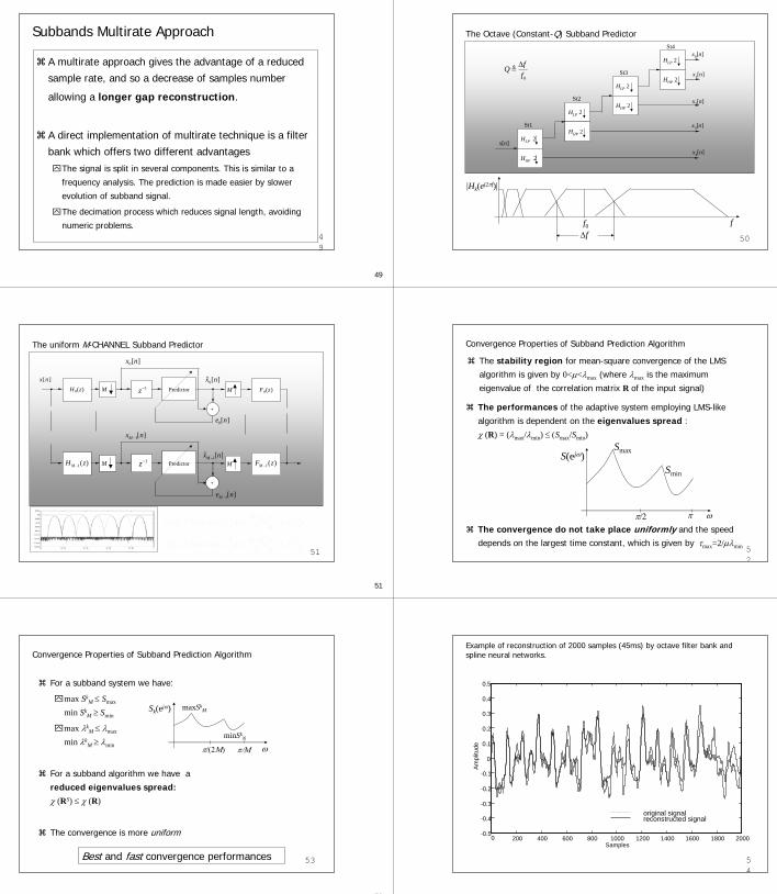
Subbands Multirate Approach

A multirate approach gives the advantage of a reduced

sample rate, and so a decrease of samples number

allowing a longer gap reconstruction.

A direct implementation of multirate technique is a filter

bank which offers two different advantagesThe signal is split in several components. This is similar to a

frequency analysis. The prediction is made easier by slower

evolution of subband signal.

The decimation process which reduces signal length, avoiding

numeric problems.49

50

The Octave (Constant-Q) Subband Predictor

50

HLP 2x[n]

HHP 2

HLP 2

HHP 2

HLP 2

HHP 2

HLP 2

HHP 2

x0[n]

x1[n]

x2[n]

x3[n]

x4[n]

St1

St2

St3

St4

0

fQf∆

∆ff0 f

|Hk(ej2πf)|

51

x [n]H0(z) M MPredictor

+

0[ ]x n

0ˆ [ ]x nF0(z)

0[ ]e n

M MPredictor

+

1[ ]Mx n−

1ˆ [ ]Mx n−

1( )MH z− 1( )MF z−

1[ ]Me n−

1z−

1z−

The uniform M-CHANNEL Subband Predictor

51

1 1[ ] 2 [ ] cos(( )[ ] ( 1) )2 2 4

ii

Nh n h n i nMπ π−

= ⋅ ⋅ + − + −

1 1[ ] 2 ( ) cos(( )[ ] ( 1) )2 2 4

ii

Nf n h n i nMπ π−

= ⋅ ⋅ + − − −

52

Convergence Properties of Subband Prediction Algorithm

The stability region for mean-square convergence of the LMS algorithm is given by 0<µ<λmax (where λmax is the maximum

eigenvalue of the correlation matrix R of the input signal)

The performances of the adaptive system employing LMS-like

algorithm is dependent on the eigenvalues spread : χ (R) = (λmax/λmin) ≤ (Smax/Smin)

The convergence do not take place uniformly and the speed depends on the largest time constant, which is given by τmax=2/µλmin

π/2 π ω

S(ejω)Smax

Smin

52

53

Convergence Properties of Subband Prediction Algorithm

For a subband system we have:

max SkM ≤ Smax

min SkM ≥ Smin

max λkM ≤ λmax

min λkM ≥ λmin

For a subband algorithm we have a

reduced eigenvalues spread:χ (RS) ≤ χ (R)

The convergence is more uniform

Best and fast convergence performances

π/(2Μ) π/Μ ω

Sk(ejω) maxSkM

minSkN

53

54

200 400 600 800 1000 1200 1400 1600 1800 2000-0.5

-0.4

-0.3

-0.2

-0.1

0

0.1

0.2

0.3

0.4

0.5

Samples

Am

plitu

de

original signalreconstructed signal

0

Example of reconstruction of 2000 samples (45ms) by octave filter bank and spline neural networks.

54

55

The MAXERR and MSE vs signal reconstructed length

0 20 40 60 80 100 120ms

0.04

0.06

0.08

0.1

0.12

0.14

0.16

0.18

0.2

0.22

0.24

Erro

r max

UFB+LPUFB+ASNNOFB+LPOFB+ASNN

0 20 40 60 80 100 120-36

-34

-32

-30

-28

-26

-24

-22

MS

E(d

B)

UFB+LPUFB+ASNNOFB+LPOFB+ASNN

ms

Best performances55

56

The subjective opinion vs signal reconstructed length

10 20 30 40 50 60 70 80 90 100 110 1202.5

3

3.5

4

4.5

5

ms

Sub

ject

ive

UFB+LPUFB+ASNNOFB+LPOFB+ASNN

Best performances56

57

Experimental Results

Signal with missing samples

57

Signal with recovered samples

58

Non liner models for sound synthesis

Natural extension of non-linear distortion synthesis technique (dynamic non linearity)

parametric control

DMLP-ASNN

signal input signal output

Feed forward scheme

Neural Networks can represent a generalization of several digital sound synthesis techniques

58

59

E.g. non linear musical oscillator (lumped circuit model)

Fairly idealized general musical oscillatorNon linear function + linear filter

⌧e(t) = f(y(t) , xE(t)) = excitation signal⌧xE(t) = external control

Energy source

e(t) y(t)

xE(t)

59

f(.)non linear active element

Resonatorlinear passive element

60

Example of a single-reed instrument

Mouthpressure

p+[n]

p-[n]

Reed

Bore Tone-hole lattice

p0[n]

REED -> External Exitation

BORE -> Resonator

BELL -> Acoustic impedance adaptation

TONE-HOLE -> Fingers control

Bell

60

61

p+[n]

p-[n]Bore Tone-hole lattice

p0[n]

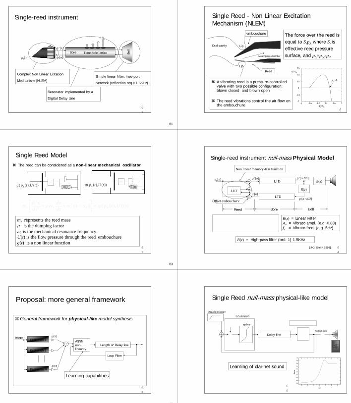
Complex Non Linear Exitation

Mechanism (NLEM)

Bell

Resonator implemented by a

Digital Delay Line

Simple linear filter: two-port

Network (reflection req.>1.5KHz)

Single-reed instrument

61

62

Single Reed - Non Linear Excitation Mechanism (NLEM)

A vibrating reed is a pressure-controlled valve with two possible configuration: blown closed and blown open

The reed vibrations control the air flow on the embouchure

Oral cavity

,r ru p

The force over the reed is equal to Srp∆ where Sr is effective reed pressure surface, and p∆=poc-pr.

Lip

Lip

Reed

embouchure

6

,oc ocu pMouthpiece chamber

-1 -0.6 -0.2 0.2 0.6 1-1

-0.5

0

0.5

1.0

1.5ur/ur0

pr/pC

p∆=0

63

The reed can be considered as a non-linear mechanical oscillator

22

02 ( ) ( ( ), ( ))r r rd x dxm x x g p t U tdt dt

µω ω ∆

⎡ ⎤+ + − =⎢ ⎥

⎣ ⎦

( ( ), ( ))g p t U t∆rm

µ

Single Reed Model

mr represents the reed massµ is the dumping factorωr is the mechanical resonance frequencyU(t) is the flow pressure through the reed embouchureg(t) is a non linear function

( ( ), ( ))g p t U t∆rm

µ

63

64

Single-reed instrument null-mass Physical Model

Offset embouchure

p+[n-N/2]p0[n]+

+

LUT

LTD

LTD

R(z)*

p+[n]

p-[n]

B(z)

p-[n+N/2]

Reed Bore Bell

1

1 ( )( ) ;1 ( )

( ) ( ) 0.642; ( ) sin(2 );v v

a tR za t z

a t v t v t A f tπ

−

+=

+= − =

R(z) = Linear FilterAv = Vibrato ampl. (e.g. 0.03)fv = Vibrato freq. (e.g. 5Hz)

B(z) = High-pass filter (ord. 1) 1.5KHz

[J.O. Smith 1993]

Non linear memory-less function

64

65

Excitation 1

Excitation M

Excitation 1

Proposal: more general framework

General framework for physical-like model synthesis

TriggerASNN non-linearity

Length N Delay line

Loop Filter

g1[n]

gM[n]

Learning capabilities

65

66

Single Reed null-mass physical-like model

⊕

Breath pressureGS neuron

Delay-line

0w

1w

Output gain

1−

spline

( )H z

1( ) 0.5(1 )H z z−= −

Learning of clarinet sound

66

67

w0

z-1

z-1

v2w1

v1

w2

z-1

z-1

w3

w4

DELAY LINEControl points

SPLINEActFunc

Breath Pressure

( )H z

IIR

FIR

One Time-Delay Spline Neuron

1 22 1

2 1 21 2

( )1a a z zH z

a z a z

− −

− −

+ +=

+ +

11( ) 0.5(1 )H z z−= −

Single Reed physical-like model

67

68

Preliminary results: Sax sound

Reed

Delay-line 1 Three-port scattering junction

( )R z

Null-mass model

Learning of clarinet and sax sounds

Sax

Three-port scattering junction

68

Delay-line 2 Delay-line 3

“Chaotic sound” behaviour

69

Preliminary results: Flute Soundembouchure

Control points

SPLINEActFunc

( )H z

Bore delay-line

mz−Breathpressure

Adaptation of the only non linear function spline parameters

69

70

Preliminary results: Trumpet sound

w0

z-1

z-1

v2w1

v1

Breathpressure

Lip filter

Delay line

α

non-linearity

Adaptable parametersα w0 w1 υ1 υ2

70

71

Another approach: additive synthesis controlled by ANN1

sgm

sgm

sgm

sgm

sgm

sgm

Loudness

F0

(1) D. Wessel, C. Drame, M. Wright, CNMAT, Berkeley

a1

a2

f1

f2

Osc.

Osc.

Osc.

Σ

Solo sax

Solo oct2

AOEUI

Suling

p1

p2

pN

fN

aN

The amplitudes and frequencies (ak ,fk) of the oscillators are controlled by a NN.

Additive SynthesizerNeural Controller

71

Note: reproduced sounds by record

72

Audio signal separationBlind separation of linear mixture

( ) = ( ) t t⋅x A s

A

s1(t)

s2(t)

sN(t)

W

x1(t)

x2(t)

xN(t)

u1(t)

u2(t)

uN(t)

g1(u1)

g2(u2)

gN(uN)

y1(t)

y2(t)

yN(t)

Unknown mixing matrix

Independent sources

Observed signals

Un-mixing matrix

Flexible activation function

Neural Network

72

Problem: estimate the un-mixing matrix W such that u(t) = s(t)(several algorithms exist).

73

73

Preliminary: signal separation of post non-linear mixture

post non-linear mixture model

A1,1

A1,2

A1,n

A2,1

A2,2

A2,n

An,1

An,2

An,n

s1(t)

s2(t)

sn(t)

u1(t)

u2(t)

un(t)

f1(.)

f2(.)

fn(.)

x1(t)

x2(t)

xn(t)

f(.)A

s(t) u(t) x(t)

W1,1

W1,2

W1,n

W2,1

W2,2

W2,n

Wn,1

Wn,2

Wn,n

v1(t)

v2(t)

vn(t)

y1(t)

y2(t)

yn(t)

W

v(t) y(t)

g1(.)

g2(.)

gn(.)

x1(t)

x2(t)

xn(t)

g(.)

x(t)

Non linear blind separation structure

,1

( ) = ( ) 1,2,...N

i i i j jj

x t f a s t i M=

⎛ ⎞=⎜ ⎟

⎝ ⎠∑

Flexible spline activation functions

74

Preliminary: signal separation of non-linear mixing

Separation of non-linear mixture

Non linear mixing model

Non linear blind separation structure

c1(t)

c2(t)

cN(t)

x1(t)

x2(t)

xN(t)

c(t) x(t)

f1(.)

f2(.)

fN(.)

u1(t)

u2(t)

uN(t)

f(.)

u(t)

BA

s1(t)

s2(t)

sN(t)

s(t)

v1(t)

v2(t)

vN(t)

y1(t)

y2(t)

yN(t)

v(t) y(t)

g1(.)

g2(.)

gn(.)

r1(t)

r2(t)

rN(t)

g(.)

r(t)

WZ

x1(t)

x2(t)

xN(t)

x(t)

, ,1 1

( ) = ( ) 1,2,...N N

k k i i i j ji j

x t b f a s t k M= =

⎛ ⎞=⎜ ⎟

⎝ ⎠∑ ∑

74

75

Preliminary Results: signal separation of post non-linear mixing

75

x1(t)

x2(t)

x3(t)

x4(t)

y1(t)

y3(t)

y4(t)

y2(t)

1 1

2 22

3 3 3

4 4

( ) = tanh( ( ))( ) = tanh( ( ))

( ) =0.8 ( ) ( )( ) = tanh(0.9 ( ))

x t u tx t u tx t u t u tx t u t

+

0.2811 0.2926 -0.1364 0.4080-0.4608 -0.1232 -0.2025 0.24920.3908 -0.3373 -0.3908 -0.2917-0.4621 -0.4660 -0.4438 -0.3846

⎡ ⎤⎢ ⎥⎢ ⎥=⎢ ⎥⎢ ⎥⎣ ⎦

AA1,1

A1,2

A1,n

A2,1

A2,2

A2,n

An,1

An,2

An,n

s1(t)

s2(t)

sn(t)

u1(t)

u2(t)

un(t)

f1(.)

f2(.)

fn(.)

x1(t)

x2(t)

xn(t)

f(.)A

s(t) u(t) x(t)

W1,1

W1,2

W1,nW2,1

W2,2W2,n

Wn,1

Wn,2

Wn,n

v1(t)

v2(t)

vn(t)

y1(t)

y2(t)

yn(t)

W

v(t) y(t)

g1(.)

g2(.)

gn(.)

x1(t)

x2(t)

xn(t)

g(.)

x(t)

Mixed inputs De-mixed outputs

76

Some conclusions

Dynamic Neural Networks represent a new class of non-liner DSP algorithms

Fast architectures allow real time applications at high throughput rate

Learning algorithms ensure consistent design methods

A huge application fields in audio/sound processing

Neural Networks: general framework for non linear digital sound analysis/synthesis methods

76