sieve analysis: statistical methods for assessing...

Sieve Analysis: Statistical methods forassessing differential vaccine protection

against HIV types

Biostat 578A Lecture 7

Research Goal: Develop statisticalmethods for assessing from vaccineefficacy trial data how vaccine protectionmay depend on characteristics of thevarious circulating HIV-1 strains

Outline

I. Introduction to Sieve Analysis

II. Models for Sieve Analysis, Binary Endpoint(HIV infection, Yes or No)

A. Discrete HIV typesB. Continuous HIV distance

III. Models for Sieve Analysis, Failure TimeEndpoint (Time to HIV infection Diagnosis)

A. Discrete HIV typesB. Continuous HIV distance: Lecture 8

Introduction to “Sieve” Analysis

• HIV-1 extremely diverse

• How broadly does acandidate vaccine protect?

• Vaccine protection depends on whichcharacteristics of challenge virus? How so?

Phylogenetic Tree of HIV-1 Subtypes

2003 Global Map of HIV-1 Subtypes

Global Dist’n of HIV-1 Subtypes 1980-1999

Introduction

• Human trials of preventive vaccines againstheterogeneous pathogens

- hepatitis Szmuness et al. 1981- cholera Clemens et al. 1991

van Loon et al. 1993- rotavirus Lanata et al. 1989

Ward et al. 1992Ukae et al. 1994

Jin et al. 1996Rennels et al. 1996

- pneumococcus Amman et al. 1977Smit et al. 1977John et al. 1984

- influenza Govaert 1994- malaria Alonso et al. 1994

• Some of these data summarized inGilbert et al. (2001, J Clin Epidem)

Introduction

• Often no quantitative statistical assessment oftype-specific vaccine efficacy

• When there is, the interpretation and validityof the analysis is often unclear

Data

• Randomized vaccine trial

• Data collection

- Measure virus characteristics ofisolated virus from breakthroughinfections

- E.g., VaxGen trials obtained 3 sequencesfrom each infected participant, froma blood sample drawn at infection diagnosis

HIV Sequence Data

��

� � � ��! "�$#

%'&)(+**-,/.1032+4�*5.76$298;:=<>�?@<�4A6B<*C�DE<�CF<�DE<�4A6B<'G�HJI-KL:=MNDO.12+4

...TRPNNNTRRSIHIG-PGR-AFYATGEIIGDIRQ...% .�6P6$2+4�< Q7DE*-?R,S%T&)(+**-,U:=<->�?@<�4V6$<:

1. ...TRPNNNTRRRIHLG-PGR-AFYATG-IIGDIRQ...

2. ...TRPNNNTRKGIHIG-PGR-AFYATGEIIGNIRQ....

. .

217. ...TRPSNNTRKGIHIG-PGR-AFYATEEITGDIRQ...WR(=.�6$<�X*5Q7DY*-?@,S%T&)(Z*-*,U:=<->7?R<�4A6$<-:

1. ...TRPNNNTRTGVHLG-PGR-VWYATGDIIGDIRQ...

2. ...TRPNNNTRRSIHIQ-PGR-AFYAT-DIIGDIRK....

. .

119. ...TRPNNNTISKIRIR-PGRGSFYATNNIIGDIRQ...

Viral Variation Structure

0 = vaccine prototype strain

1. Nominal categorical:

K+1 distinct strains in circulation0, · · · ,K

2. Ordered categorical:

K+1 distinct strains in circulation0, · · · ,K

- ordered from prototype strain 0

3. Continuous:

Each strain is a continuous distance fromprototype strain 0

• A vast number of meaningful ways tostructure pathogen variation

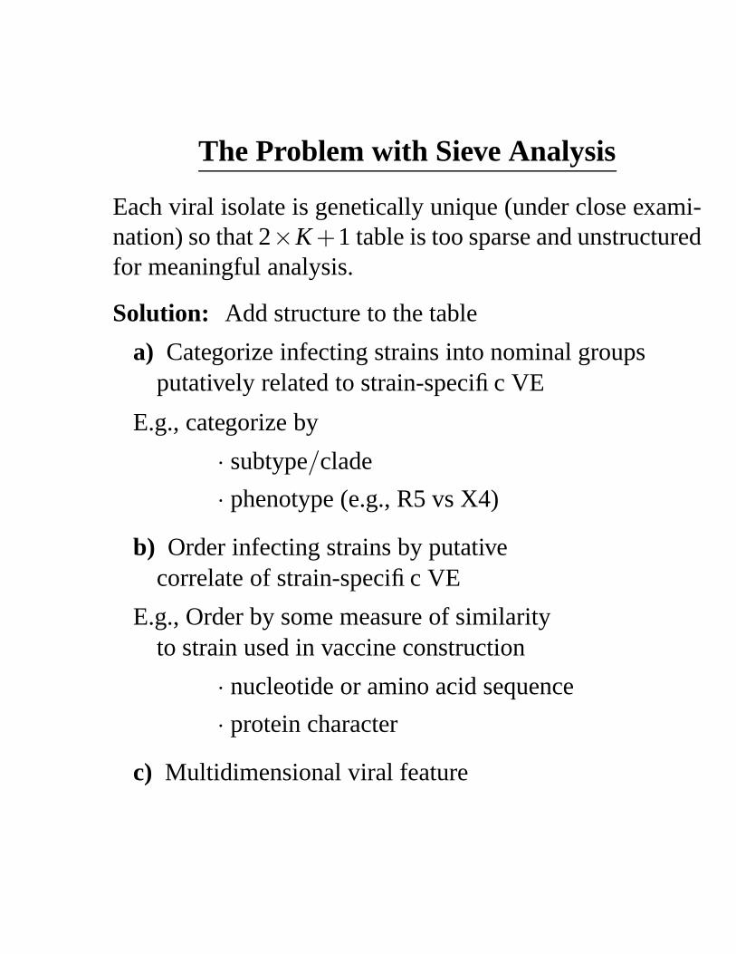
The Problem with Sieve Analysis

Each viral isolate is genetically unique (under close exami-nation) so that 2×K +1 table is too sparse and unstructuredfor meaningful analysis.

Solution: Add structure to the table

a) Categorize infecting strains into nominal groupsputatively related to strain-specific VE

E.g., categorize by

· subtype/clade

· phenotype (e.g., R5 vs X4)

b) Order infecting strains by putativecorrelate of strain-specific VE

E.g., Order by some measure of similarityto strain used in vaccine construction

· nucleotide or amino acid sequence

· protein character

c) Multidimensional viral feature

Categorical Model for Sieve Analysis

• Counts data

Infecting strains1 2 · · · · · · K

PlaceboVaccine

• Assume K +1 viral strainsin circulation

• Nominal or ordinal response

Multinomial Logistic Regression Model(Cox, 1970; Anderson, 1972)

Pr(Y = s|x) =exp{αs +β T

s x}

1+∑K

l=1exp{αl +β T

l x}

s = 0, · · · ,K; α0 = β0 ≡ 0

• Generalized linear logit model

log

{Pr(Y = s|x)Pr(Y = 0|x)

}= αs +β T

s x

• Interpretation of regression parameters:

βs = log{

Pr(Y=s|vacc)Pr(Y=0|vacc)/

Pr(Y=s|plac)

Pr(Y=0|plac)

}

= log{OR(s)}

Model Properties

• Minimal assumptions

• Estimation by maximum likelihood

• Exact methods an option

Hirji (1992, JASA, 87)

Computing Exact Distributions forPolytomous Response Data

Strain-Specific Vaccine Efficacy

• Define “per strain-specific contact”vaccine efficacy by V E pc(s) = 1−RRpc(s)

where

RRpc(s) =Pr (Inf|Expos. to strain s,Vaccine)Pr (Inf|Expos. to strain s,Placebo)

• RRpc(s) has an interpretation interms of biological vaccine efficacy

Prospective Interpetation of RegressionModel Parameters

Assumptions1. Infection is possible from at most

one strain during follow-up

2. The relative prevalence of strains isconstant over time

3. Equal exposure of vaccine and control groups

4. Pr(Infection|Exp to strain s ,V ) = exp{α0s + γsV}

−→ βs = γs

(Proof in Gilbert, Self, and Ashby, 1998, Biometrics)———————————————————————

• OR(s) = RRpc(s)RRpc(0)

• βs = log{

RRpc(s)RRpc(0)

}

• βs−βt = log{

RRpc(s)RRpc(t)

}

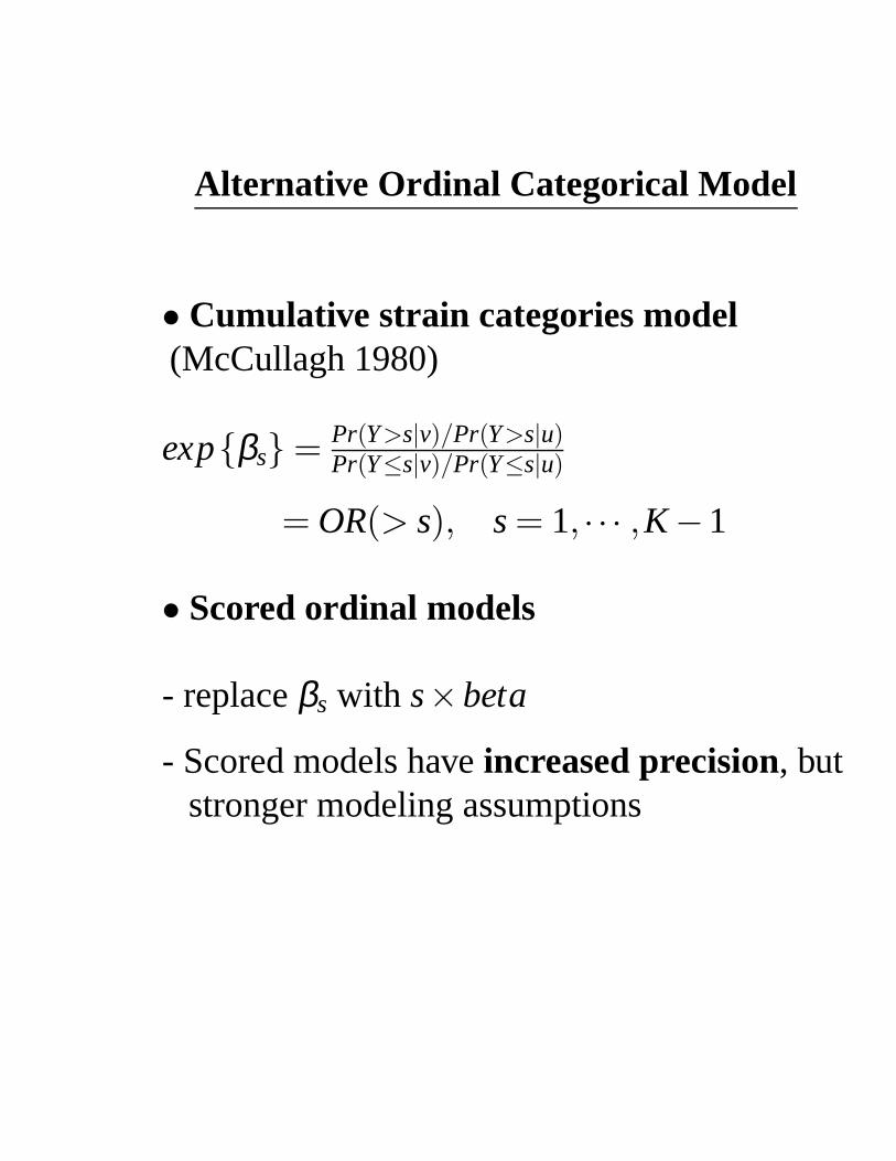
Alternative Ordinal Categorical Model

• Cumulative strain categories model(McCullagh 1980)

exp{βs} = Pr(Y>s|v)/Pr(Y>s|u)Pr(Y≤s|v)/Pr(Y≤s|u)

= OR(> s), s = 1, · · · ,K −1

• Scored ordinal models

- replace βs with s×beta

- Scored models have increased precision, butstronger modeling assumptions

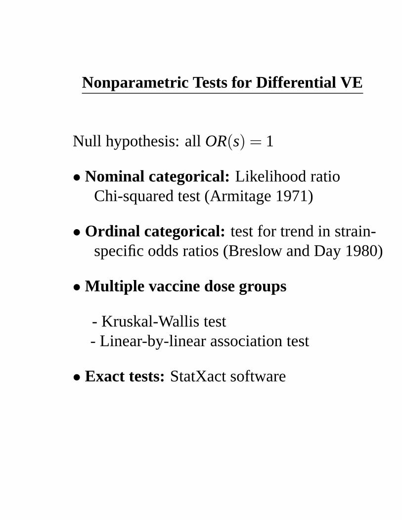
Nonparametric Tests for Differential VE

Null hypothesis: all OR(s) = 1

• Nominal categorical: Likelihood ratioChi-squared test (Armitage 1971)

• Ordinal categorical: test for trend in strain-specific odds ratios (Breslow and Day 1980)

• Multiple vaccine dose groups

- Kruskal-Wallis test- Linear-by-linear association test

• Exact tests: StatXact software

Parametric Tests for Differential V E

• MLR or cumulative categories

Null hypothesis: all βs = 0

- likelihood ratio Chi-squared test- Zelen’s test (1991)

Finer null hypothesis: a subset of β ′ss = 0

• Categorical scored modelsNull hypothesis: β = 0

• Continuous modelNull hypothesis: β = 0

- likelihood ratio, Wald, and score test

Example

• Hepatitis B vaccine trial in New York(Szmuness et al., 1981)

HepatitisB A non-A,B

Placebo 63 27 11 101Vaccine 7 21 16 44

- Likelihood ratio statistic: χ22 = 30.2, p < 0.0001

RRpc(A)RRpc(B)

= 7.0 (2.7,18.4) 95% CI

RRpc(non−A,B)RRpc(B)

= 13.1 (4.3,39.3) 95% CI

Example

• Ordered categorical viral feature:

Number sub/del to the prototypehexapeptide tip sequence of V3 loop

E.g., VaxGen’s MN/GNE8 rgp120 vaccine:

GPGRAF

Estimate

RRpc(1 sub/del)RRpc(GPGRAF)

RRpc(2 sub/del)RRpc(GPGRAF)

RRpc(3+ sub/del)RRpc(GPGRAF)

Generalized Logistic Regression Model(Gilbert et al., 1999, 2000)

• Continuous analog of MLR model

- parameterized MLR model: βs = g(s)θ

g a deterministic function

• Generalized Logistic Regression (GLR) model:

Pr(Y = y|vaccine) = exp{g(y)θ} f (y)∫ ∞0 exp{g(z)θ}dF(z)

f (y) ≡ Pr(Y = y|placebo)

• Parametric component:

regression relationship

• Nonparametric component:

baseline strain distribution F

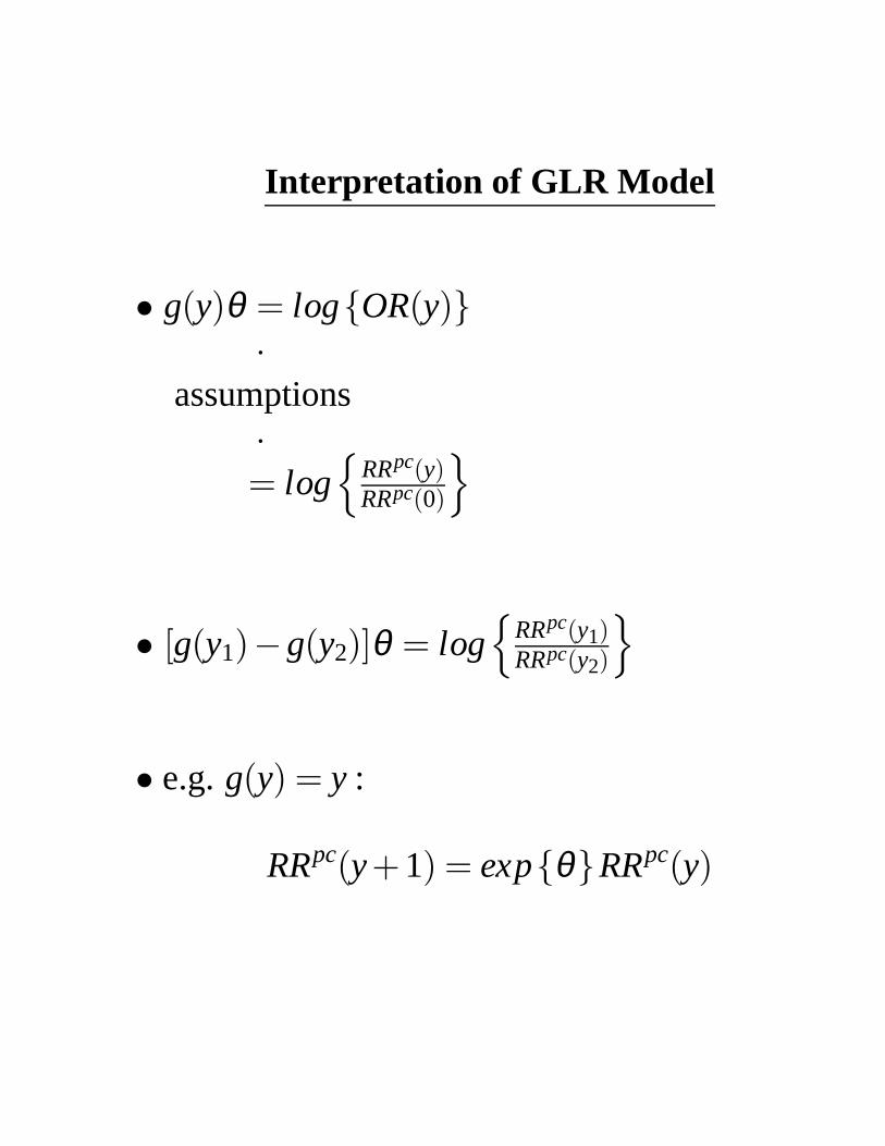
Interpretation of GLR Model

• g(y)θ = log{OR(y)}·

assumptions·= log

{RRpc(y)RRpc(0)

}

• [g(y1)−g(y2)]θ = log{

RRpc(y1)RRpc(y2)

}

• e.g. g(y) = y :

RRpc(y+1) = exp{θ}RRpc(y)

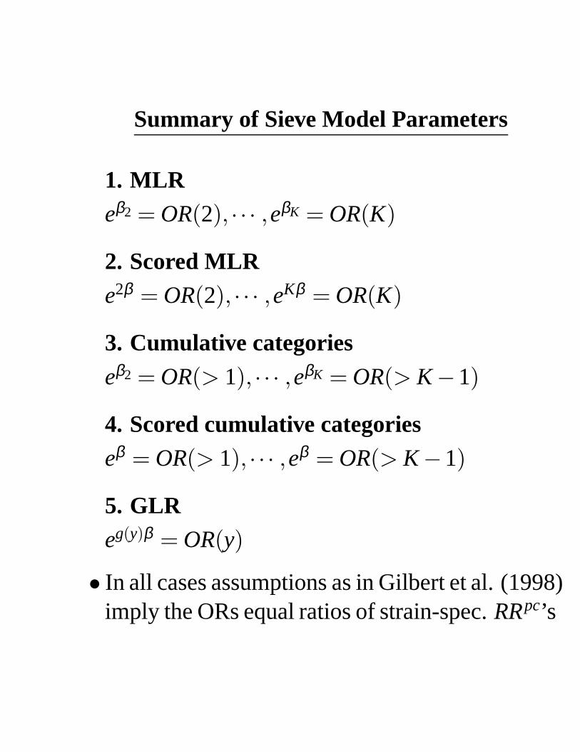
Summary of Sieve Model Parameters

1. MLReβ2 = OR(2), · · · ,eβK = OR(K)

2. Scored MLRe2β = OR(2), · · · ,eKβ = OR(K)

3. Cumulative categories

eβ2 = OR(> 1), · · · ,eβK = OR(> K −1)

4. Scored cumulative categorieseβ = OR(> 1), · · · ,eβ = OR(> K −1)

5. GLReg(y)β = OR(y)

• In all cases assumptions as in Gilbert et al. (1998)imply the ORs equal ratios of strain-spec. RRpc’s

Multidimensional Pathogen Variation

• The MLR and GLR models can accomodatepathogen variation described bymultiple features

• Examples

1. cholera: biotype, serotype, diseaseseverity

2. rotavirus: serotype, disease severity

3. HIV-1: vast possibilities

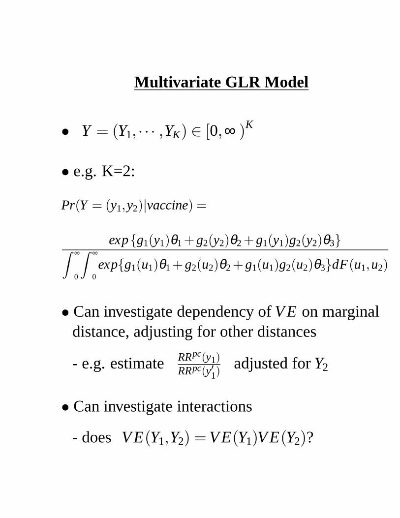
Multivariate GLR Model

• Y = (Y1, · · · ,YK) ∈ [0,∞ )K

• e.g. K=2:

Pr(Y = (y1,y2)|vaccine) =

exp{g1(y1)θ1 +g2(y2)θ2 +g1(y1)g2(y2)θ3}∫ ∞

0

∫ ∞

0exp{g1(u1)θ1 +g2(u2)θ2 +g1(u1)g2(u2)θ3}dF(u1,u2)

• Can investigate dependency of V E on marginaldistance, adjusting for other distances

- e.g. estimate RRpc(y1)RRpc(y′1)

adjusted for Y2

• Can investigate interactions

- does V E(Y1,Y2) = V E(Y1)V E(Y2)?

Example

• Merck’s Adenovirus-5 vaccinevector

- includes core proteins coded bygag, pol, and nef

• Y = (Ygag,Ypol,Yne f )

Ygag a metric based on gagYpol a metric based on polYne f a metric based on nef

• Investigate how vaccine protection depends onheterogeneity in gag, pol, and nef

Example

• Question: What are the roles of CD4+cellular responses and CD8+ cellular responsesin conferring homologous and heterologousprotection?

• Y = (YCD4+,YCD8+)

YCD4+ = strength of CD4+ T helper responseagainst the vaccine strain- a T help metric

YCD8+ = strength of CD8+ T cell responseagainst the vaccine strain- a CTL metric

Example

• Six-variate GLR model: Investigatecorrelation of Merck’s Ad 5 vaccine protectionwith MHC Class I and Class II T cellresponses against gag, pol, and nef

(gag, pol,ne f )× (CD4+,CD8+)

Y = (YCD4+,gag, YCD4+,pol, YCD4+,ne f ,YCD8+,gag, YCD8+,pol, YCD8+,ne f)

s-sample GLR Model

• s distinct covariate groups

x1, · · · ,xs

Pr(Y = y|xi) =exp

{∑d

k=1gik(y)θk

}f (y)

∫ ∞

0exp

{∑d

k=1gik(u)θk

}dF(u)

• multiple vaccine dose groups

• stratify by covariates

• adjust for low-dimensional covariates

Estimation in GLR Model

• Maximum likelihood estimation

• s−sample GLR model is asemiparametric biased sampling model:

Pr(Y = y|i) =wi(y,θ ) f (y)∫ ∞

0wi(u,θ )dF(u)

, i = 1, · · · ,s

-e.g. two-sample GLR model:

w1(y,θ ) ≡ 1, w2(y,θ ) = exp{g(y)θ}

Partial Likelihood Estimation

• Partial likelihood

Ln1(θ ,V ) =s

∏i=1

ni

∏j=1

[λniwi(yi j,θ )Vi

∑s

k=1λnkwk(yk j,θ )Vk

]

with Vi ≡1

Wi(F,θ)

Maximization Algorithm

1. Maximize Ln1 over θ and V, V > 0

2. Compute Vardi’s (1985) NPMLE F̂n

using ‘known’ weight functions wi(·, θ̂n)

Properties of MLE in GLR Model

• Described in Gilbert et al. (1999,Biometrika; 2000, Ann Stat)

• GLR model identifiable

• GLR model uniquely estimable- log profilepartial likelihood strictly concave

•(θ̂n, F̂n) uniformly consistent, asymptotically

normal, and asymptotically efficient

• Confidence intervals and variance estimation

1. sample estimator of generalized Fisherinformation

2. bootstrap

• Satisfactory finite-sample properties

• Comparable to MLE in Cox model

Simulation Study of Gilbert et al. (1999)

• Study performance of (θ̂n, F̂n)

• Investigate bias and estimation of variancevia observed inverse generalised Fisherinformation and via the bootstrap

• Investigate power of likelihood ratio,Wald and score tests of H0 : θ = 0(no differential vaccine protection), andcoverage accuracy of corresponding CIs


• Y = percent amino acid differencebetween an infecting virus and theglobal subtype B consensus in the V3 loop

• Specify true log RR ratio as

log{RRpc(y)/RRpc(0)} =y

35θ

-Set θ = 0,2, and 4

θ = 0 : RRpc(35) = 1.0RRpc(0)

θ = 2 : RRpc(35) = 7.39RRpc(0)

θ = 4 : RRpc(35) = 54.6RRpc(0)


• Consider 4 baseline distribution functions F

- Unif(0,35)

- Normal(0.1157,0.7102)

- Expon(0.1157/2)

- Thai empirical (based on 94 sequences)

- 0.1157 and 0.710 based on 159 subtype B V3loop sequences in the LANL database

• 4 sample sizes (numbers of infections):(np,nv)= (100,100),(100,50),(50,50),(50,25)

• Simulations based on 1000 trials

æ[�xî �ª� è#�r�r��4��h´�³Y��r��4�4��<��Ò�´ æs�#î Ð ��h�)�r��4��h´r³Y��4�4��<��Ò�´

strain distance (%)

coun

t

0 10 20 30 40

0

10

20

30

40

50

strain distance (%)

coun

t

0 20 40 60 80

0

10

20

30

40

50

� ��<��ê�æ[�xî¦��rÒÄ²��<��r��4�4��<��Ò�´GÒhÑ/��<� ó R ��Ò{Òh��h��´<Ò��h³O��Ø�r��4��h´r³Y�¾��O�§²��O�|´Üê �hì �ª� è#��<�r�§Ô°�� õ �4�|ä{�<�|´r³Y�|� �h´r�¤��<�¾��Òh��h�,��<�r�§Ô°�� õ ³YÒ�´r�4�|´��r�*�4�|ä{�<�|´r³Y�h�uæs�#î��<Ò¬²��*��<��4�4��<��Ò�´�ÒhÑ�ì ��ó R ��Ò{Òh�Ø�h��i´<Ò�h³O��r��h´r³Y�|�(ÒhÑ5��´<Ñs�|³Y��´<��4�4��h�i´r�(��´ Ð �r�h�i��h´r�)�

1 �

Ð �W��êW� a�cdTfeªTW]�o¯mWTWVnc[TW]#j�Q�^`_�Xsy<QªZT�hcsZ�zUZ® c¨«hQO® c¨y{^|^ÄoØQneYX[c¨Z�ThXg^WV C�<ö �$]rcsX�Q ��eOTWZ R�®�Q�mfTWVncdTW]�j�QÓ ( � ^��YeOQYVnmWQ�oÀ°QO]#QYV4TW®±cie|Q�o $cie�yUQYV�c¨]|_O^WVnZ�ThX[c[^h]wmfTWVncdTW]�j�QQYenX[csZ�ThX�Q�� ^|^hXseYX[V`TnRqmfThV�cdTW]�jnQ

QOX[csZ�ThX�Q�� / �u´r��ÑsÒh�� / * Òh��\�h�O $ O � � ��G � Ó Ó ( �� G � Ó Ó ( ��

ê '$' ê '$' ' � '"2 '<ê '"2 1 � '"2 1 � '"2 1 ' � '"2 ' R '"2 � � '"2 �(' '"2 R+R�(' 1 � ' � '"2 '$' '"2 �{ê '"2 � � '"2 � 1 '"2 1 � ê#2 1 ê ê#2 �� '"2 ì��ê '$' ê '$' 1 '"2 ' 1 '"2 R ' '"2 1 ì '"2 R ' � '"2 '<ê '"2 � 1 '"2 � � '"2 � ��(' 1 � 1 '"2 '�í '"2 ì � '"2 ì�� ê#2 '<ê '"2 1 ' ê#2 � R ê#2 �{ê ê#2 �Wíê '$' ê '$' � '"2 '�í '"2 � ì '"2 � � '"2 � í '"2 '<ê '"2 �� '"2 � � '"2 � 1�(' 1 � � '"2 1 � ê#2 í � ê#2 � � ê#2 �$� '"2 1 ì 1 2 1 í 1 2�ê � 1 2 � �

/ ��ß{��Ò�´<�|´°��h� / Ð �r�h�O $ O � � ��G � Ó Ó�( �� G � Ó Ó ( �� ê '$' ê '$' ' '"2 '*� '"2 � � '"2 �Wì '"2 � � '"2 '<ê '"2 � ì '"2 � 1 '"2 R í�(' 1 � ' '"2 R í ê#2 � í 1 2 � ì ê#2 �� '"2 1 ê ê#2 1 � ê#2 � R '"2 ì �ê '$' ê '$' 1 '"2 ' � '"2 � � '"2 � � '"2 � � '"2 ' � '"2 � � '"2 � R '"2 � ��(' 1 � 1 '"2�ê ' ê#2 �hí ê#2 ìUê ê#2 ì 1 '"2�ê 1 ê#2 í(' ê#2 �� ê#2 ��ê '$' ê '$' � '"2 ' � '"2 � � '"2 �� '"2 � � '"2 '�ì '"2 � � '"2 � 1 '"2 ��(' 1 � � '"2 1+R ê#2 ì � ê#2 í � 1 2 1 � '"2 1 � 1 2�ê|ì ê#2 ì�� 1 2 1+R

1 ê

Ð �W�� 1 � �*^WÂ�QOVª^`_�®±c¨«hQY®±c¨y{^|^|oÕV4ThX[cd^fk��KTW®�o¤Th]�o\eYj�^hV4Q�X�QYenXseª^`_ � � �%�.� ' Â5csXsy�� '�2 ' �/ �u´r��ÑsÒh�� * Òh��\�h� �5ßU�#Ò�´r�|´x��h� Ð �r�h�O $ O � � , -��W��Ò , - �W��Ò , -��W��Ò Þw�h�� èU³YÒh�� , -��W��Ò

ê '$' ê '$' ' '"2 ' � '"2 ' � '"2 ' 1 '"2 ' 1 '"2 ' � '"2 ' ��(' 1 � ' '"2 ' � '"2 ' R '"2 ' 1 '"2 ' 1 '"2 ' � '"2 ' Rê '$' ê '$' 1 '"2 ì � '"2 íUê '"2 �Wì '"2 �$� '"2 í�� '"2 í ��(' 1 � 1 '"2 �Uê '"2 � ' '"2 R � '"2 R+R '"2 �Uê '"2 � êê '$' ê '$' � ê#2 '$' ê#2 '$' ê#2 '$' ê#2 '$' ê#2 '$' ê#2 '$'�(' 1 � � '"2 ìhì '"2 ì R '"2 ìhì '"2 ì � '"2 ìhì '"2 ì 1

1$1

Ð �W�� R � �#j�^WV�Q�enXgThX[c¨enX[cdj�j�^h]��oxQO]�j�Q�cs]�X�QOV�mWTW® eªT��^Wz<X �� ' 2 ' �/ �u´r��ÑsÒh�� * Òh��h� ��ß{��Ò�´<�|´°��h� Ð �r�h�O $ O � �

ê '$' ê '$' ' ��ê#2�ê �{Ö�ê#2�ê 1 ��ê#2 ��{Ö�ê#2 �hí ��ê#2 R í{Ö�ê#2 í � ��ê#2 � R Ö�ê#2 íhí�(' 1 � ' ��ê#2 �hí{Ö 1 2�ê � ��ê#2 íUêWÖ R 2 R � ��ê#2 �{êWÖ R 2�ê � ��ê#2 �('UÖ R 2 '*�ê '$' ê '$' 1 '"2 ì R Ö R 2 ' R '"2 ��{Ö R 2 � ì '"2 � 1 Ö R 2 �hì '"2 � 1 Ö R 2 �hí�(' 1 � 1 '"2 1 í{Ö � 2 '<ê � '"2�ê �{Ö � 2 � 1 '"2�ê|í{Ö � 2 ì 1 � '"2�ê 1 Ö � 2 �híê '$' ê '$' � 1 2 �$�°Ö � 2 �(' 1 2 �hí{Ö � 2 � R R 2 '<êWÖ � 2 �Wí 1 2 � R Ö � 2�êhê�(' 1 � � ê#2 íUêWÖ � 2 �(' ê#2 � �°Ö � 2 1 � 1 2 R+R Ö � 2 � ê ê#2 �hì{Ö � 2 �Wí

1+R

••••••••••••••••••••••••••••••••••••••••••••••••••••••••••••••••••••••••••••••••••••••••••••••••••••

-4 -2 0 2 4

-15

-10

-5

0

-0.00

F uniform

••••••••••••••••••••••••••••••••••••••

••••••••••••••••••••••••••••••••••••••••••••••••••••••••••••••

0 2 4 6 8

-6

-1

4

9

3.96

F uniform

0.01,0.32

F uniform

2.05,3.76

F uniform

••••••••••••••••••••••••••••••••••••

••••••••••••••••••••••••••••••••••••••••••••••••••••••••••••••••

-4 -2 0 2 4

-14

-9

-4

1

0.062

F normal

••••••••••••••••••••••••••••••••

•••••••••••••••

•••••••••••••••••••••••••••••••••••••••••••••••••••••

0 2 4 6 8

-9

-4

1

6

3.98

F normal

0.18,-0.16

F normal

2.57,3.97

F normal

•••••••••••••••••••••••••••

•••••••••••••

••••••••••••••••••••••••••••••••••••••••••••••••••••••••••••

-4 -2 0 2 4

-15

-10

-5

0

-0.00

F exponential

•••••••••••••••••••••••••••••••••••••••

•••••••••••••••••••••••••••••••••••••••••••••••••••••••••••••

0 2 4 6 8

-8

-3

2

7

3.95

F exponential

0.30,0.05

F exponential

2.16,3.91

F exponential

••••••••••••••••••••••••••••

•••••••••••••

•••••••••••••••••••••••••••••••••••••••••••••••••••••••••••

-4 -2 0 2 4

-15

-10

-5

0

-0.04

F Thai

•••••••••••••••••••••••••••••••••

•••••••••••••••••••••••••••••••••••••••••••••••••••••••••••••••••••

0 2 4 6 8

-9

-4

1

6

3.98

F Thai

0.05,0.22

F Thai

2.27,3.85

F Thai

� ��<� 1 �$��rÒÄ²��(��r��Òh��r��ÒWÙ#��b��W��h�)��µh�|��<Ò{Ò{�¯�h�O��r� ��ÑsÒh��4��|³Y�4��r�AÒhÑ+�h�|´<�O��W�4�|�Ø�r�W��4�O��O� Ð �<�¾Òh�r��h��´<�|� C�\��¦²*��4�4�|´Ø�W�#Ò¬�h��|�h³��K��Òh�O� Ð �<�bÙ��4�(�§²�ÒG³YÒ��r��´r�(�W��Òh��(ÑsÒh�*��<��²�ÒW��h��r��Òh��|�A��O�r��|��|´x��´r��h�� O� O $ � ê '$' �7O � � �(' ��h´r�¤��<��|³YÒ�´r�¤��²�Ò

³YÒ��r��´��(�W��Òh��¦ÑsÒh��r�¾��<��O�Y��h��¾�r��Òh��|�A��O�r��|�4�|´°��´<��h��¾��O�O $ �1ê '$' �7O � $ � �(' �7O � ( � 1 � �

1 �

••••••••••••••••••••••••••••••••••••

distance

Fha

t(di

stan

ce)

0 10 20 30

0.0

0.2

0.4

0.6

0.8

1.0

(a) F uniform, asymptotic CIs

••••••••••••••••••••••••••••••••••••

distance

Fha

t(di

stan

ce)

0 10 20 30

0.0

0.2

0.4

0.6

0.8

1.0

(b) F uniform, bootstrap CIs

•••••••••••••••••

••••••••••••••••••••••

••••••

••••••••••••••••••••••••••

distance

Fha

t(di

stan

ce)

0 10 20 30 40

0.0

0.2

0.4

0.6

0.8

1.0

(c) F normal, asymptotic CIs

•••••••••••••••••

••••••••••••••••••••••

••••••

••••••••••••••••••••••••••

distance

Fha

t(di

stan

ce)

0 10 20 30 40

0.0

0.2

0.4

0.6

0.8

1.0

(d) F normal, bootstrap CIs

•

•

•

•

•

•

•••••••

•••••

••••••••••••••••••••••••••••••••••••••••••••••••••••••••••

distance

Fha

t(di

stan

ce)

0 10 20 30 40

0.0

0.2

0.4

0.6

0.8

1.0

(e) F expon, asymptotic CIs

•

•

•

•

•

•

•••••••

•••••

••••••••••••••••••••••••••••••••••••••••••••••••••••••••••

distance

Fha

t(di

stan

ce)

0 10 20 30 40

0.0

0.2

0.4

0.6

0.8

1.0

(f) F expon, bootstrap CIs

••

•

•

•

•

•

•

••

••

••

• • • •

distance

Fha

t(di

stan

ce)

10 20 30 40 50 60

0.0

0.2

0.4

0.6

0.8

1.0

(g) F Thai, asymptotic CIs

••

•

•

•

•

•

•

••

••

••

• • • •

distance

Fha

t(di

stan

ce)

10 20 30 40 50 60

0.0

0.2

0.4

0.6

0.8

1.0

(h) F Thai, bootstrap CIs

� ��<� R �$�#Òh��4��|ÔU�*�r�W��O��*�h�|´<�O��W�4�|�KÑs��Ò�� O $ �1ê '$' �7O � � �(' �� 1 � æ[�xî�Öiæ[³Äî�Öiæs�¬î �h´r�Üæs�°î(��<Ò¬²��<��|�h´¤ÒhÑ C/ �h³Y��Ò��*��<�Gê '$'$'��O��i��³O�W��Ò�´r�OÖU²��ì�� ) �4ÔU��O�4��i³u�h��Ô{��4Òh��³�´<Òh��\�h��W�r�r��ÒÄßU��\�W��Ò�´¤³YÒ�´UÙ��<�|´�³Y��h´r�r�|� Ð �<�¾�4��<��r�i�4�4��r��Ò�´G�i�(�<�O��³Y�4�|�¤�{ÔÕ��4Ò��¤�i��´<�h�

æs�#î�Öiæ[�#î�ÖiæsÑ�î(�h´r�wæ[��î(��´r³O��r�r�bì�� ) �#Ò{Òh��4�4��W�K³YÒ�´UÙ��<�|´r³Y�¾��h´r�r�O�

1 �

Pseudo-Example from Gilbert et al. (1999)

• Generated a single dataset usingthe empirical Thai strain distributionand assuming that:

V E pc(y ≤ 0.10) = 50%

V E pc(0.11 ≤ y ≤ 0.20) = 40%

V E pc(0.21 ≤ y ≤ 0.30) = 30%

V E pc(0.31 ≤ y ≤ 0.40) = 20%

V E pc(0.41 ≤ y ≤ 0.50) = 10%

V E pc(0.51 ≤ y) = 0%

• Number of infections np = 100,nv = 69

• Fit the same GLR model studied in simulations

• LR, Wald and score tests: p = 0.10,0.10,0.09

•••••••••••••••••••••••••••••••••••••••••••••••••••••••••••••••••••••••••••••••••••••••••••••••••••••••••••••••••••••••••••••••••••••••••••••••••••••••••••••••••••••••••••••••••••••

•••••••••••••••••••••••••••••••••••••••••••••••••••••••••••••••••••••••••••••••••••••••••••••••••••••••••••••••••••••••••••••••••••••••••

•••••••••••••••••••••••••••••••••••••••••••••••••••••••••••••••••••••••••••••••••••••••••••••••••••••••••••••

•••••••••••••••••••••••••••••••••••••••••••••••••••••••••••••••••••••••••••••••••••••••••••

••••••••••••••••••••••••••••••••••••••••••••••••••••••••••••••••••••••••••••••

•••••••••••••••••••••••••••••••••••••••••••••••••••••••

strain distance

RR

(dis

tanc

e)/R

R(0

)

0 10 20 30 40 50 600

1

2

3

••

••

••

(a) Vaccine protection versus strain distance

• • • ••

••

•• • • • • • • • • •

strain distance

cum

ulat

ive

prob

abili

ty

10 20 30 40 50 600.0

0.2

0.4

0.6

0.8

1.0

• • • •• •

•

•• • • • • • • • • •

(b) NPMLE Fhat and F versus strain distance

� ��<� � � æ[�xî(��<ÒÄ² �(��<�¾�|�4��\�W�4�|�¤��W��Ò�ÒhÑ/��|��W��h�¾��4µU� ��æ��<î76 ��æ 'xî��h�O��r�*�4�4��h��´¤�r��4��h´�³Y� ��h� ��4Ò��Õ��i´<�h� Ð �<�¾�r��Òhµh�|´Ø��´<�|�(�W��r��ÒWÙ��¾��µh�|��<Ò{Ò{�<�g��h�4�|�¯³YÒ�ÚÙ��<�|´r³Y��i´x�4�O��W�h��OÖr�h´��¤��<��<Òh�4�4�|�Ø��i´<�¾�4�4�O�Ñ[�r´r³Y��Ò�´¤��*��<�¾�4��<��|��W��h�¾��µ\��W��Ò<�uæs�#î��<Ò¬²�� C/ �h��4Ò��¤��i´<�|�OÖU²��ì�� )

�h�4Ô{��r�4Òh��³�´<Òh��h�)�W�r�r��ÒÄßU�i��W��Ò�´³YÒ�ÚÙ#�<�|´r³Y�¾��h´r��(�h��<Òh��*�r�h��<�|��i��´<�|�¦�h´r�Øì�� )��Ò°Òh��4��W�Ø³YÒ�ÚÙ��r�|´r³Y�¾��h´r�r�(�h� ��Ò�´<��r�h��<�|��´r�|�O� Ð �<�b�4��<� / ��¦��Òh��4��|Ôh�|�K�h��<Òh�4�4�|�Ø��´<�|�O�

1 �

III. Incorporating Time to Infection Diagnosis

• Cause-specific hazards approachPrentice et al. (1978, Biometrics);foundational paper

- Suppose K circulating strains

- Let Y1, · · · ,YK be conceptual or latentinfection Dx times corresponding to the K strains

- Classic competing risks data: Data areiid observations (Ti,δi,Si,zi)

Ti = min(Y1, · · · ,YK)δi = failure indicator (1 if infected)Si = infecting strain (NA if not infected)zi = covariate vector

Cause-specific Hazards

• Prentice et al. (1978) emphasized that allfunctions of cause-specific hazards λs areestimable from the data (Ti,δi,Si,zi)

λs(t|z) =lim4t↘0Pr(t ≤ T < t +4t,S = s|T ≥ t,z)

4t

Cause-Specific Proportional Hazards Model

• Prentice et al. (1978) proposed a cause-specificproportional hazards model:

λs(t|z) = exp{

β Ts z

}λs(t|0)

- arbitrary baseline hazard λs(t|0)- when z is vaccination status,

βs = log{λs(t|vaccine)/λs(t|placebo)}

- βs = log-relative hazard (vaccine vs placebo)of infection by strain s

- V E(s) ≡ 1− exp{βs} measures strain-specificvaccine efficacy

• βs can be estimated by the standard maximumpartial likelihood estimator (MPLE), treatinginfection by all non-s strains as censoring

Interpretation of βs

• λs has a “crude” interpretation,which is restricted to the particular vaccinetrial conditions

• Additional assumptions needed for the strains-specific vaccine efficacy estimate

V̂ E(s) = 1− exp{β̂s}

to have a meaningful biological interpretation

• Would like V E(s) = V E pc(s), whereV E pc(s) is one minus the relative conditionalprobability (vaccine vs placebo) of a specifiedamount of exposure to strain s causingHIV infection


• Assumptions:A1: For each strain s ∈ {1, · · · ,K},the probability of infection with strain sresulting from a specified amount of exposureis homogeneous and constant over time amongvaccinated and placebo subjects, so thatvaccination reduces the transmission probabilityby the same fraction exp{γs}for all vaccinees (i.e., “leaky” protection againsteach strain; Halloran, Haber, and Longini, 1992)

A2: The pattern of risk behavior and exposureto each strain s ∈ {1, · · · ,K} during thefollow-up period [0,τ] for a trial participant isthe same whether vaccine or placebo wasassigned (justified by randomization andblinding)


• Under A1 and A2, the crude hazard ratio

exp{β} =λs(t|vaccine)λs(t|placebo)

equals the biologically interpretable parameter

exp{γs} = 1−V E pc(s)

• Therefore, under A1 and A2 the MPLE β̂s in thestrain s-specific proportional hazards modelestimates γs (and V̂ E(s) estimates V E pc(s))

• Based on Rhodes, Halloran, and Longini(1992, JRSS B), under randomization andblinding, β̂s should be ≈ unbiasedif the strain s infection rate is low

Sketch of Proof (from Gilbert, 2000, Stat Med)

λs(t|z) = λEs(t|z)×Pr(t ≤ T < t +4t,S = s|T ≥ t,z,

exposed to strain s in [t, t +4t)),

-λEs(t|z) is the Markov intensity of the countingprocess counting exposures to strain s forparticipants with covariate z

-The second term conditions on a specifiedexposure during [t, t +4t),e.g., on a sexual or needle contact with astrain s-infected individual

Sketch of Proof (from Gilbert, 2000, Stat Med)

• A1 implies a constant strain-specifictransmission probability over time in each group

• A2 implies λEs(t|vacc) = λEs(t|plac) for all t

• Together these results imply βs = γs

• Therefore the MPLE β̂s in the strain s-specificproportional hazards model estimates γs

Assessing Differential Protection

• Since each γs is estimated from a separate modelfit, the strain-specific proportional hazardsmodels do not permit direct comparisons ofvaccine efficacy across strains

• Lunn and McNeil (1995, Biometrics) showedhow to reparametrize the strain s Cox modelso that exp{βs} (s ≥ 2) equals

λs(t|v)λs(t|u)

/λ1(t|v)λ1(t|u)

- βs measures relative vaccine efficacy againststrain s compared to the reference strain 1

• Therefore standard Cox model software (e.g.,in Splus/R) can be used to estimate βs witha confidence interval

Tests for Vaccine Efficacy Against Strain s

• Standard Cox model software provides tests of

H0haz : λs(t|vaccine) = λs(t|placebo)

- Through creative coding also provides tests of

H0 : V E(1) = V E(2)

• An alternative to a hazards-based approachwould apply Gray’s (1988, Ann Stat) methodto test different cumulative incidence functions,H0ci : Fvs = Fps, where

Fvs(t) = Pr(T ≤ t,S = s|vaccine)

Fps(t) = Pr(T ≤ t,S = s|placebo)

Example: Oral Cholera Vaccine Trial

• A randomized double-blind field trial wasconducted in rural Bangladesh among childrenover 2 years and adult women (1985-1992)

• Assessed the efficacy of B subunit killed wholecell (BSWC) and killed whole-cell-only (WC)oral cholera vaccines

• Case endpoint: First diarrheal episode in whichVibrio cholerae 01 was isolated

• 2 cholera biotypes (classical, El Tor) and2 cholera serotypes (Inaba, Ogawa)circulated during the trial

- The causal infecting biotype and serotypewas measured for each case

Example: Oral Cholera Vaccine Trial

• Analysis of the study population of 62,285children and women who received three dosesthe BSWC vaccine (20,705), the WC vaccine(20,743), or the Escherichia coliK12 strain placebo (20,837)

• Overall the two vaccines performed similarly

- Each vaccine had about 50% efficacy sustainedfor 2 or 3 years, waning to nill at 5 years

Cum. Inc. of Strain-Specific Cholera Casesch

oler

a ca

ses

classical,n=157El Tor,n=108

050

100

150

May‘85 May‘86 May‘87 May‘88

Placebo

chol

era

case

s


050

100

150


WC Vaccine

chol

era

case

s


050

100

150


BSWC Vaccine

chol

era

case

s

classical Ogawa,n=135El Tor Ogawa,n=94classical Inaba,n=22El Tor Inaba,n=14

050

100

150


Placebo

chol

era

case

s


050

100

150


WC Vaccine

chol

era

case

s


050

100

150


BSWC Vaccine

Biotype-specific 1-Cum. Inc. Curves

disease free time (days since third dose)

prop

ortio

n no

t dis

ease

d

0 200 400 600 800 10000.99

00.

994

0.99

8

classicalEl Tor Placebo

WC Vaccine

Placebo

WC Vaccine


prop

ortio

n no

t dis

ease

d

0 200 400 600 800 10000.99

00.

994

0.99

8

classicalEl Tor Placebo

BS WC Vaccine

Placebo

BS WC Vaccine

Biotype/Serotype-specific 1-Cum. Inc. Curves


prop

ortio

n no

t dis

ease

d

0 200 400 600 800 10000.99

00.

994

0.99

8

classical, OgawaEl Tor, Ogawa

Placebo

WC Vaccine

Placebo

WC Vaccine


prop

ortio

n no

t dis

ease

d

0 200 400 600 800 10000.99

850.

9990

0.99

951.

0000

classical, InabaEl Tor, Inaba

Placebo

WC Vaccine

Placebo

WC Vaccine


prop

ortio

n no

t dis

ease

d

0 200 400 600 800 10000.99

00.

994

0.99

8

classical, OgawaEl Tor, Ogawa

Placebo

BS WC Vaccine

Placebo

BS WC Vaccine


prop

ortio

n no

t dis

ease

d

0 200 400 600 800 10000.99

850.

9990

0.99

951.

0000

classical, InabaEl Tor, Inaba

Placebo

BS WC Vaccine

Placebo

BS WC Vaccine

Sieve Analyses to Assess Differential Protection

• Conducted sieve analysis to compare V E(1) andV E(2) (where 1 and 2 indicate differentbiotypes or serotypes) using 4 methods:

1. MLR model

2. MLR model stratified by the 3 years offollow-up (account for temporal trends inshifting biotype/serotype prevalence)

3. Cause-specific Cox model with Lunn andMcNeil recoding

4. Cause-specific Cox model with Lunn andMcNeil recoding and with a proportionalbaseline risks assumption λ1(t|0) = λ2(t|0)

• For cause-specific Cox model, results obtainedusing standard coxph function in Splus/R

Fit of Sieve Models to Cholera Data

• Compare V E for El Tor vs Classical

Vaccine Model β̂ a SE(β̂) Robust SE(β̂ ) exp{β̂} =̂exp{γEl}

exp{γcl}95% CIb P-value

WC MLR 0.421 0.217 1.524 (0.946,2.332) 0.052WC Stratified MLR 0.389 0.219 1.475 (0.961,2.265) 0.076WC PHc 0.433 0.217 0.218 1.541 (1.006,2.360) 0.047WC PH, PBRd 0.428 0.217 0.217 1.534 (1.002,2.347) 0.049

BS WC MLR 0.359 0.215 1.432 (0.940,2.181) 0.095BS WC Stratified MLR 0.318 0.221 1.375 (0.891,2.122) 0.150BS WC PH 0.369 0.215 0.212 1.446 (0.949,2.204) 0.085BS WC PH, PBR 0.365 0.215 0.212 1.440 (0.946,2.194) 0.089

a β = γEl Tor− γclassicalb95% CIs derived from a normality approxima-tion and the information matrixcPH model fit by duplication Method B of Lunnand McNeildPH model fit under the proportional baseline risksassumption by duplication Method A of Lunn andMcNeil

Summary of Results

• For each vaccine, the 4 methods performsimilarly

- Result explained by the very low failure rate

• Results suggest that both vaccines protect≈ 50% better against classical thanEl Tor cholera

• A possible explanation is that thevaccine contains 3 times as many Classicalas El Tor antigens

Summary of Utility of Sieve Analysis Methods

1. Statistical inference of differential vaccineprotection according to a pathogen variationstructure chosen a priori

2. Exploratory tools for identifying whichpathogen features are potentially correlatedwith vaccine protection

sieve analysis: statistical methods for assessing...

Documents