siam j. s comput c vol. 36, no. 4, pp. c335–c352€¦a parallel directional fast multipole method...

Copyright © by SIAM. Unauthorized reproduction of this article is prohibited.

SIAM J. SCI. COMPUT. c© 2014 Society for Industrial and Applied MathematicsVol. 36, No. 4, pp. C335–C352

A PARALLEL DIRECTIONAL FAST MULTIPOLE METHOD∗

AUSTIN R. BENSON† , JACK POULSON‡ , KENNETH TRAN§ , BJORN ENGQUIST¶, AND

LEXING YING‖

Abstract. This paper introduces a parallel directional fast multipole method (FMM) for solvingN-body problems with highly oscillatory kernels, with a focus on the Helmholtz kernel in three di-mensions. This class of oscillatory kernels requires a more restrictive low-rank criterion than that ofthe low-frequency regime, and thus effective parallelizations must adapt to the modified data depen-dencies. We propose a simple partition at a fixed level of the octree and show that, if the partitionsare properly balanced between p processes, the overall runtime is essentially ON logN/p + p. By thestructure of the low-rank criterion, we are able to avoid communication at the top of the octree. Wedemonstrate the effectiveness of our parallelization on several challenging models.

Key words. parallel, fast multipole methods, N-body problems, scattering problems, Helmholtzequation, oscillatory kernels, directional, multilevel

AMS subject classifications. 65Y05, 65Y20, 78A45

DOI. 10.1137/130945569

1. Introduction. This paper is concerned with a parallel algorithm for the rapidsolution of a class of N -body problems. Let {fi, 1 ≤ i ≤ N} be a set of N densitieslocated at points {pi, 1 ≤ i ≤ N} in R

3, with |pi| ≤ K/2, where | · | is the Euclideannorm and K is a fixed constant. Our goal is to compute the potentials {ui, 1 ≤ i ≤ N}defined by

(1.1) ui =

N∑j=1

G(pi, pj) · fj ,

where G(x, y) = e2πι|x−y|/|x − y| is the Green’s function of the Helmholtz equation.We have scaled the problem such that the wavelength equals one and thus high fre-quencies correspond to problems with large computational domains, i.e., large K.

The computation in (1.1) arises in electromagnetic and acoustic scattering, wherethe usual partial differential equations are transformed into boundary integral equa-tions (BIEs) [16, 25, 40, 42]. The discretized BIEs often result in large, dense linearsystems with N = O(K2) unknowns, for which iterative methods are used. Equa-tion (1.1) represents the matrix-vector multiplication at the core of the iterative meth-ods.

∗Submitted to the journal’s Software and High-Performance Computing section November 18,2013; accepted for publication (in revised form) May 5, 2014; published electronically August 14,2014. This work was partially supported by National Science Foundation under award DMS-0846501and by the Mathematical Multifaceted Integrated Capability Centers (MMICCs) effort within theApplied Mathematics activity of the U.S. Department of Energy’s Advanced Scientific ComputingResearch program, under Award number(s) DE-SC0009409.

http://www.siam.org/journals/sisc/36-4/94556.html†ICME, Stanford University, Stanford, CA 94305 ([email protected]). This author’s work

was supported by an Office of Technology Licensing Stanford Graduate Fellowship.‡Department of Mathematics, Stanford University, Stanford, CA 94305 ([email protected]).§Microsoft Corporation, Redmond, WA 98052 ([email protected]).¶Department of Mathematics and ICES, University of Texas at Austin, Austin, TX 78712

([email protected]).‖Department of Mathematics and ICME, Stanford University, Stanford, CA 94305 (lexing@math.

stanford.edu).

C335

Dow

nloa

ded

08/1

8/14

to 1

71.6

7.21

6.21

. Red

istr

ibut

ion

subj

ect t

o SI

AM

lice

nse

or c

opyr

ight

; see

http

://w

ww

.sia

m.o

rg/jo

urna

ls/o

jsa.

php

http://www.siam.org/journals/sisc/36-4/94556.html

mailto:[email protected]







C336 BENSON, POULSON, TRAN, ENGQUIST, AND YING

1.1. Previous work. Direct computation of (1.1) requires O(N2) operations,which can be prohibitively expensive for large values of N . A number of methods re-duce the computational complexity without compromising accuracy. The approachesinclude FFT-based methods [2, 3, 6], local Fourier bases [4, 8], Chebyshev inter-polation [28], and the high-frequency fast multipole method (HF-FMM) [9, 13, 33].Another related development is the butterfly algorithm [18, 29, 30]. We focus onthe directional FMM [19, 20, 21, 39]. The directional FMM exploits the numericallylow-rank interaction satisfying a directional parabolic separation condition, which isfundamentally different than the approach in HF-FMM.

There are several methods for parallel FMM on nonoscillatory kernels [17, 24, 32,45], and recent work provides a scalable parallel butterfly algorithm [31]. The kernel-independent fast multipole method (KI-FMM) [43] is a central tool for our algorithmin the “low-frequency regime,” which we will discuss in subsection 2.3. Many effortshave extended KI-FMM to modern, heterogeneous architectures [11, 12, 32, 44, 46],and several authors have paralellized [22, 23, 37, 41] the multilevel fast multipolealgorithm [15, 35, 36], which is a variant of the HF-FMM.

1.2. Contributions. This paper provides the first parallel algorithm for com-puting (1.1) based on the directional FMM algorithm. The top of the octree imposesa well-known bottleneck in parallel FMM algorithms for the low-frequency case [44].A key advantage of our approach is that the interaction lists of boxes in the high-frequency regime with width greater than or equal to 2

√K are empty. This alleviates

the bottleneck, as no translations are needed at those levels of the octree. However,the directional interactions between points in the high-frequency regime are compli-cated, and this makes parallelization challenging.

Our parallel algorithm is based on a partition of the boxes at a fixed level in theoctree amongst the processes (see subsection 3.1). Due to the structure of directionalFMM in the high-frequency regime, we can leverage the partition into a flexible par-allel algorithm. The parallel algorithm is described in section 3, and the results ofseveral numerical experiments are in section 4. As will be seen, the algorithm exhibitsgood strong scaling up to 1024 processes for several challenging models.

2. Preliminaries. In this section, we review the directional low-rank property ofthe Helmholtz kernel and the sequential directional algorithm for computing (1.1) [19].Proposition 2.1 in subsection 2.2 shows why the algorithm can avoid computation atthe top levels of the octree. We will use this to develop the parallel algorithm insection 3.

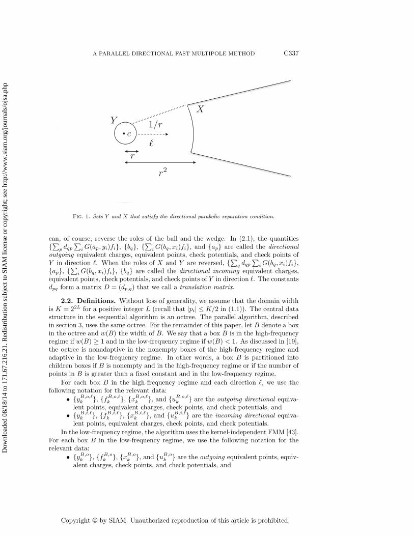
2.1. Directional low-rank property. Let Y be a ball of radius r ≥√3 cen-

tered at a point c, and define the wedge X = {x : θ(x, �) ≤ 1/r, |x− c| ≥ r2}, where �is a unit vector and θ(x, �) is the angle between the vectors x and �. The sets Y and Xare said to satisfy the directional parabolic separation condition, which is illustratedin Figure 1.

Suppose we have a set of charges {fi} located at points {yi} ⊆ Y . Given athreshold ε, there exist two sets of points {bq}1≤q≤rε

and {ap}1≤p≤rεand a set of

constants {dpq}1≤p,q≤rεsuch that, for x ∈ X ,

(2.1)

∣∣∣∣∣∑i

G(x, yi)fi −∑q

G(x, bq)

(∑p

dqp∑i

G(ap, yi)fi

)∣∣∣∣∣ = O(ε),

where rε is a constant that depends only on ε. A random sampling method based onthe pivoted QR factorization [21] can be used to determine this approximation. We

Dow

nloa

ded

08/1

8/14

to 1

71.6

7.21

6.21

. Red

istr

ibut

ion

subj

ect t

o SI

AM

lice

nse

or c

opyr

ight

; see

http

://w

ww

.sia

m.o

rg/jo

urna

ls/o

jsa.

php


A PARALLEL DIRECTIONAL FAST MULTIPOLE METHOD C337

1/r

r

YX

c

X

r2

Fig. 1. Sets Y and X that satisfy the directional parabolic separation condition.

can, of course, reverse the roles of the ball and the wedge. In (2.1), the quantities{∑

p dqp∑

iG(ap, yi)fi}, {bq}, {∑

iG(bq, xi)fi}, and {ap} are called the directionaloutgoing equivalent charges, equivalent points, check potentials, and check points ofY in direction �. When the roles of X and Y are reversed, {

∑q dqp

∑iG(bq, xi)fi},

{ap}, {∑

i G(bq, xi)fi}, {bq} are called the directional incoming equivalent charges,equivalent points, check potentials, and check points of Y in direction �. The constantsdpq form a matrix D = (dp,q) that we call a translation matrix.

2.2. Definitions. Without loss of generality, we assume that the domain widthis K = 22L for a positive integer L (recall that |pi| ≤ K/2 in (1.1)). The central datastructure in the sequential algorithm is an octree. The parallel algorithm, describedin section 3, uses the same octree. For the remainder of this paper, let B denote a boxin the octree and w(B) the width of B. We say that a box B is in the high-frequencyregime if w(B) ≥ 1 and in the low-frequency regime if w(B) < 1. As discussed in [19],the octree is nonadaptive in the nonempty boxes of the high-frequency regime andadaptive in the low-frequency regime. In other words, a box B is partitioned intochildren boxes if B is nonempty and in the high-frequency regime or if the number ofpoints in B is greater than a fixed constant and in the low-frequency regime.

For each box B in the high-frequency regime and each direction �, we use thefollowing notation for the relevant data:

• {yB,o,�k }, {fB,o,�

k }, {xB,o,�k }, and {uB,o,�

k } are the outgoing directional equiva-lent points, equivalent charges, check points, and check potentials, and

• {yB,i,�k }, {fB,i,�

k }, {xB,i,�k }, and {uB,i,�

k } are the incoming directional equiva-lent points, equivalent charges, check points, and check potentials.

In the low-frequency regime, the algorithm uses the kernel-independent FMM [43].For each box B in the low-frequency regime, we use the following notation for therelevant data:

• {yB,ok }, {fB,o

k }, {xB,ok }, and {uB,o

k } are the outgoing equivalent points, equiv-alent charges, check points, and check potentials, and

Dow

nloa

ded

08/1

8/14

to 1

71.6

7.21

6.21

. Red

istr

ibut

ion

subj

ect t

o SI

AM

lice

nse

or c

opyr

ight

; see

http

://w

ww

.sia

m.o

rg/jo

urna

ls/o

jsa.

php



• {yB,ik }, {fB,i

k }, {xB,ik }, and {uB,i

k } are the incoming equivalent points, equiv-alent charges, check points, and check potentials.

Due to the translational and rotational invariance of the relevant kernels, the(directional) outgoing and incoming equivalent and check points can be efficientlyprecomputed since they only depend upon the problem size, K, and the desired ac-curacy.1 We discuss the number of equivalent points and check points in subsection4.1.

Let B be a box with center c and w(B) ≥ 1. We define the near field of a boxB in the high-frequency regime, NB, as the union of boxes A that contain a pointin a ball centered at c with radius

√3w/2. Such boxes are too close to satisfy the

directional parabolic condition described in subsection 2.1. The far field of a box B,FB, is simply the complement of NB. The interaction list of B, IB, is the set ofboxes NP \NB, where P is the parent box of B.

To exploit the low-rank structure of boxes separated by the directional paraboliccondition, we need to partition FB into wedges with a spanning angle of O(1/w).To form the directional wedges, we use the construction described in [19]. The con-struction has a hierarchical property: for any directional index � of a box B, thereexists a directional index �′ for boxes of width w(B)/2 such that the �th wedge of B iscontained in the �′th wedge of B’s children. Figure 2 illustrates this idea. In order toavoid boxes on the boundary of two wedges, the wedges are overlapped. Boxes thatwould be on the boundary of two wedges are assigned to the wedge that comes firstin an arbitrary lexicographic ordering.

2.3. Sequential algorithm. In the high-frequency regime, the algorithm usesdirectional M2M, M2L, and L2L translation operators [19], similar to the standardFMM [14]. The high-frequency directional FMM operators are as follows:

• HF-M2M constructs the outgoing directional equivalent charges of B fromthe outgoing equivalent charges of B’s children,

• HF-L2L constructs the incoming directional check potentials of B’s childrenfrom the incoming directional check potentials of B, and

• HF-M2L adds to the incoming directional check potentials of B due to out-going directional charges from each box A ∈ IB.

The following proposition shows that at the top levels of the octree, the interactionlists are empty.

Proposition 2.1. Let B be a box with width w. If w ≥ 2√K, then NB contains

all nonempty boxes in the octree.Proof. Let c be the center of B. Then for any point pi ∈ B, |pi − c| ≤

√3w/2.

For any point pj in a box A, |pj − c| ≤ |pj | + |pi| + |pi − c| ≤ K +√3w/2. NB

contains all boxes A such that there is an x ∈ A with |x − c| ≤ 3w2/4. Thus,NB will contain all nonempty boxes if 3w2/4 ≥

√3w/2 + K. This is satisfied for

w ≥√4K/3 + 1/3 +

√1/3. Since K = 22L, this simplifies to w ≥ 2

√K.

Thus, if w(B) ≥ 2√K, no HF-M2L translations are performed (IB = ∅). As a

consequence, no HF-M2M or HF-M2L translations are needed for those boxes. Thisproperty of the algorithm is crucial for the construction of the parallel algorithm thatwe present in section 3.

We denote the corresponding low-frequency translation operators as LF-M2M,LF-L2L, and LF-M2L. We also denote the interaction list of a box in the low-frequency

1Our current hierarchical wedge decomposition does not respect rotational invariance, and so, insome cases, this precomputation can be asymptotically more expensive than the subsequent direc-tional FMM.

Dow

nloa

ded

08/1

8/14

to 1

71.6

7.21

6.21

. Red

istr

ibut

ion

subj

ect t

o SI

AM

lice

nse

or c

opyr

ight

; see

http

://w

ww

.sia

m.o

rg/jo

urna

ls/o

jsa.

php



WB,

WC,

B

C

w

3w2

3w2/4

Fig. 2. A two-dimensional slice of the three-dimensional hierarchical wedges. WB,� is thewedge for box B for the directional index �. By the hierarchical construction, we can find an index

direction �′ such that for any child box C of B, WB,� is contained in WC,�′ , the �′th wedge of C.Since C has a smaller width (w) than B (2w), the wedge for C is closer and wider than the wedgefor B. This is a consequence of the directional parabolic separation condition described in subsection2.1.

regime by IB, although the definition of NB is different [19]. Algorithm 1 presents thesequential algorithm in terms of the high- and low-frequency translation operators.

3. Parallelization. The overall structure of our proposed parallel algorithm issimilar to the sequential algorithm. A partition of the boxes at a fixed level in theoctree governs the parallelism, and this partition is described in subsection 3.1. Weanalyze the communication, computation, and spatial complexities in subsections 3.4,3.5, and 3.6. For the remainder of this paper, we use p to denote the total number ofprocesses.

3.1. Partitioning the octree. To parallelize the computation, we partition theoctree at a fixed level. Suppose we number the levels of the octree such that the lthlevel consists of a 2l × 2l × 2l grid of boxes of width K · 2−l. By Proposition 2.1,there are no dependencies between boxes with width strictly greater than

√K. The

partition assigns a process to every box B with w(B) =√K, and we denote the

partition by P . In other words, for every nonempty box B at level L in the octree(recall that K = 22L), P(B) ∈ {0, 1, . . . , p − 1}. We refer to level L as the partitionlevel. Process P(B) is responsible for all computations associated with box B and thedescendent boxes of B in the octree, and so we also define P(A) ≡ P(B) for any boxA ⊂ B. An example partition is illustrated in Figure 3.

Dow

nloa

ded

08/1

8/14

to 1

71.6

7.21

6.21

. Red

istr

ibut

ion

subj

ect t

o SI

AM

lice

nse

or c

opyr

ight

; see

http

://w

ww

.sia

m.o

rg/jo

urna

ls/o

jsa.

php



Algorithm 1: Sequential directional FMM for (1.1).

Data: points {pi}1≤i≤N , densities {fi}1≤i≤N , and octree TResult: potentials {ui}1≤i≤N

foreach box B in postorder traversal of T with w(B) < 1 doforeach child box C of B do

Transform {fC,ok } to {fB,o

k } via LF-M2M

foreach box B in postorder traversal of T with 1 ≤ w(B) ≤√K do

foreach direction � of B doLet the �′th wedge of B’s children contain the �th wedge of Bforeach child box C of B do

Transform {fC,o,�′k } to {fB,o,�

k } via HF-M2M

foreach box B in preorder traversal of T with 1 ≤ w(B) ≤√K do

foreach direction � of B doforeach box A ∈ IB in direction � do

Let �′ be the direction for which B ∈ IA

Transform {fA,o,�′k } via HF-M2L and add result to {uB,i,�

k }foreach child box C of B do

Transform {uB,i,�k } to {uC,i,�

k } via HF-L2L

foreach box B in preorder traversal of T with w(B) < 1 doforeach A ∈ IB do

Transform {fA,ok } via LF-M2L and add the result to {uB,i

k }Transform {uB,i

k } via LF-L2Lif B is a leaf box then

foreach pi ∈ B doAdd result to ui

elseforeach child box C of B do

Add result to {uC,ik }

There are two reasons for using this partitioning. First, the partition leads tosimple communication patterns (see the following subsection), which results in smallcommunication time for practical problems (see section 4). Second, with minimalcommunication, running time is dominated by the translation computations. In sub-section 3.5, we show that as long as we can partition boxes evenly at the partitionlevel, the work is balanced. There are more sophisticated process distributions in simi-lar tree computations [26], but the communication costs and scalability for directionalFMM on nonuniform geometries are unclear.

3.2. Communication. We assume that the ownership of point and densitiesconforms to the partition P , i.e., each process owns exactly the points and densitiesneeded for its computations. In practice, arbitrary point and density distributionscan be handled with a simple preprocessing stage. Our later experiments make use ofk-means clustering [27] to distribute the points to processes. This clustering can be

Dow

nloa

ded

08/1

8/14

to 1

71.6

7.21

6.21

. Red

istr

ibut

ion

subj

ect t

o SI

AM

lice

nse

or c

opyr

ight

; see

http

://w

ww

.sia

m.o

rg/jo

urna

ls/o

jsa.

php



Fig. 3. Two-dimensional slice of the octree at the partition level for a spherical geometry witheach box numbered with the process to which it is assigned. The width of the boxes at the partitionlevel is

√K, which ensures that the interaction lists of all boxes above this partition level are empty.

We note that the number of boxes with surface points (black border) is much smaller than the totalnumber of boxes.

used as a heuristic for creating P (see subsection 4.2).

The partition P dictates the communication in our algorithm. Since P(C) = P(B)for any any child box C of B, there is no communication for the L2L or M2M trans-lations in both the low-frequency and high-frequency regimes. These translations areperformed in serial on each process. All communication is induced by the M2L trans-lations. In particular, for every box A ∈ IB for which P(A) = P(B), process P(B)needs outgoing (directional) equivalent densities of box A from process P(A). Wedefine IB = {A ∈ IB|P(A) = P(B)}, i.e., the set of boxes in B’s interaction list thatdo not belong to the same process as B. The parallel algorithm performs two bulkcommunication steps:

1. After the HF-M2M translations are complete, all processes exchange outgoingdirectional equivalent densities. The interactions that induce this communi-cation are illustrated in Figure 4. For every box B in the high-frequencyregime and for each box A ∈ IB , process P(B) requests fA,o,� from processP(A), where � is the index of the wedge for which B ∈ IA.

2. After the HF-L2L translations are complete, all processes exchange outgoingnondirectional equivalent densities. For every box B in the low-frequencyregime and for each box A ∈ IB, process P(B) requests fA,o from processP(A).

Alternatively, the algorithm could communicate equivalent densities for the LF-M2L and HF-M2L translations at each level in the preorder traversal of the octree. Intheory, this provides an opportunity to overlap computation and communication toimprove performance. However, in the numerical experiments of section 4, we showthat the communication time is minimal. Using the bulk communication keeps the

Dow

nloa

ded

08/1

8/14

to 1

71.6

7.21

6.21

. Red

istr

ibut

ion

subj

ect t

o SI

AM

lice

nse

or c

opyr

ight

; see

http

://w

ww

.sia

m.o

rg/jo

urna

ls/o

jsa.

php



0 0

0 0

2 2

2 2

1 1

1 1

1

2

2

1

3w2/4w

Fig. 4. Interaction in the high-frequency regime that induces communication in the parallelalgorithm. In this case, process 0 needs outgoing directional equivalent densities in direction �1from process 1 and direction �2 from process 2. The equivalent densities are translated to incomingdirectional potentials in the directions �′1 and �′2 via HF-M2L. Similarly, processes 1 and 2 needoutgoing directional equivalent densities in directions �′1 and �′2 from process 0.

algorithm simple without sacrificing performance.

3.3. Parallel algorithm. We finally arrive at our proposed parallel algorithm.Communication for the HF-M2L translations occurs after the HF-M2M translationsare complete, and communication for the LF-M2L translations occurs after the HF-L2L translations are complete. The parallel algorithm from the view of process q isin Algorithm 2. We assume that communication is not overlapped with computation.Although there is opportunity to hide communication by overlapping, the overallcommunication time is small in practice, and the more pressing concern is properload balancing (see section 4).

3.4. Communication complexity. We will now discuss the communicationcomplexity of our algorithm assuming that the N points are quasi-uniformly sampledfrom a two-dimensional manifold with N = O(K2), which is generally satisfied formany applications which involve boundary integral formulations. In the followingproposition, we consider the setting of a constant number of points sampled perwavelength (λ) for a fixed geometry. We note, however, that the implementation ofthe algorithm does not depend on this sampling rate. Instead of analyzing smaller λ,we fix λ = 1 and scale the geometry by 1/λ = K.

Proposition 3.1. Let S be a surface in B(0, 1/2). Suppose that for a fixed K, thepoints {pi, 1 ≤ i ≤ N} are samples of KS, where N = O(K2) and KS = {K ·p|p ∈ S}(the surface obtained by magnifying S by a factor of K). Then, for any prescribedaccuracy, the proposed algorithm sends at most O(K2 logK) = O(N logN) data inaggregate.

Outline of the proof. We analyze the amount of data communicated at each oftwo steps.

• We claim that at most O(N logN) data is communicated for HF-M2L. Weknow that, for a box B of width w, the boxes in its high-frequency inter-action list are approximately located in a ball centered at B with radius

Dow

nloa

ded

08/1

8/14

to 1

71.6

7.21

6.21

. Red

istr

ibut

ion

subj

ect t

o SI

AM

lice

nse

or c

opyr

ight

; see

http

://w

ww

.sia

m.o

rg/jo

urna

ls/o

jsa.

php



Algorithm 2: Parallel directional FMM for (1.1) from the view of process q.

Data: points {pi}1≤i≤N , densities {fi}1≤i≤N , octree T , partition PResult: potentials {ui}1≤i≤N

foreach box B in postorder traversal of T with w(B) < 1,P(B) = q doforeach child box C of B do

// P(C) = P(B) = q, so child data is available locally

Transform {fC,ok } to {fB,o

k } via LF-M2M

foreach box B in postorder traversal of T with 1 ≤ w(B) ≤√K,P(B) = q do

foreach direction � of B doLet the �′th wedge of B’s children contain the �th wedge of Bforeach child box C of B do


Transform {fC,o,�′k } to {fB,o,�

k } via HF-M2M

// High-frequency M2L data communication

foreach box B with w(B) > 1 and P(B) = q doforeach box A ∈ IB do

Let � be the direction for which B ∈ IA

Request fA,o,� from process P(A)

foreach box B in preorder traversal of T with 1 ≤ w(B) ≤√K,P(B) = q do

foreach direction � of B doforeach box A ∈ IB in direction � do

Let �′ be the direction for which B ∈ IA

Transform {fA,o,�′k } via HF-M2L and add result to {uB,i,�

k }foreach child box C of B do


Transform {uB,i,�k } to {uC,i,�

k } via HF-L2L.

// Low-frequency M2L data communication

foreach box B with w(B) ≤ 1 and P(B) = q doforeach box A ∈ IB do

Request fA,o from process P(A)

foreach box B in preorder traversal of T with w(B) < 1,P(B) = q doforeach A ∈ IB do

Transform {fA,ok } via LF-M2L and add the result to {uB,i

k }Transform {uB,i

k } via LF-L2Lif B is a leaf box then

foreach pi ∈ B doAdd result to ui

else// P(C) = P(B) = q, so child data is available locally

foreach child box C of B do

Add result to {uC,ik }

Dow

nloa

ded

08/1

8/14

to 1

71.6

7.21

6.21

. Red

istr

ibut

ion

subj

ect t

o SI

AM

lice

nse

or c

opyr

ight

; see

http

://w

ww

.sia

m.o

rg/jo

urna

ls/o

jsa.

php



3w2/4 and that there are O(w2) directions {�}. The fact that our pointsare samples from a two-dimensional manifold implies that there are at mostO(w4/w2) = O(w2) boxes in B’s interaction list. Each box in the interactionlist contributes at most a constant amount of communication. Since the pointsare sampled from a two-dimensional manifold, there are O(K2/w2) boxes ofwidth w. Thus, each level in the high-frequency regime contributes at mostO(K2) communication. We haveO(logK) levels in the high-frequency regime(w = 1, 2, 4, . . . ,

√K), so the total communication volume for HF-M2L is at

most O(K2 logK) = O(N logN).• In the low-frequency regime, there are O(N) boxes, and the interaction listof each box is of a constant size. Thus, at most O(N) data is communicatedfor LF-M2L.

The constants in the above analysis strongly depend on the geometry of the prob-lem. Specifically, the number of boxes in the octree that contain surface points variesby geometry. This has implications for scalability, which we explore theoretically insubsection 3.7 and empirically in subsection 4.2.

To analyze the cost of communication, we use a common model: each processcan simultaneously send and receive a single message at a time, and the cost of send-ing a message with n units of data is α + βn [1, 10, 38]. The constant α is thestart-up cost, or latency, and β is the inverse bandwidth. At each of the two commu-nication steps, each process needs to communicate with every other process. If thecommunication is well-balanced at each level of the octree, i.e., the amount of datacommunicated between any two processes is roughly the same, then the communica-tion is similar to an “all-to-all” or “index” pattern. The communication time is thenO(pα+ 1

pK2 logKβ) or O(log pα+ log p

p K2 logKβ) using standard algorithms [5, 38].We emphasize that, while we have not shown that such balanced partitions even al-ways exist, if the partition P clusters the assignment of boxes to processes, then manyboxes in the interaction lists are already owned by the correct process. This tends toreduce communication, and in practice, the actual communication time is small (seesubsection 4.2).

3.5. Computational complexity. Our algorithm parallelizes all of the trans-lation operators, which constitute nearly all of the computations. This is a directresult from the assignment of boxes to processes by P . However, the computationalcomplexity analysis depends heavily on the partition. We will make idealizing as-sumptions on the partitions to show how the complexity changes with the number ofprocesses, p.

Recall that we assume that communication and computation are not overlapped.Thus, the translations are computed simultaneously on all processes.

Proposition 3.2. Suppose that each process has the same number boxes in thelow-frequency regime. Then the LF-M2M, LF-M2L, and LF-L2L translations havecomputational complexity O(N/p).

Proof. Each nonempty box requires a constant amount of work for each of thelow-frequency translation operators since the interaction lists are of constant size.There are O(N) boxes in the low-frequency regime, so the computational complexityis O(N/p) if each process has the same number of boxes.

We note that Proposition 3.2 makes no assumption on the assignment of thecomputation to process at any fixed level in the octree: we need only a load-balancedpartition throughout all of the boxes in the low-frequency regime. It is important tonote that empty boxes (i.e., boxes that do not contain any of the {pi}) require no

Dow

nloa

ded

08/1

8/14

to 1

71.6

7.21

6.21

. Red

istr

ibut

ion

subj

ect t

o SI

AM

lice

nse

or c

opyr

ight

; see

http

://w

ww

.sia

m.o

rg/jo

urna

ls/o

jsa.

php



computation. When dealing with two-dimensional surfaces in three dimensions, thisposes a scalability issue (see subsection 3.7).

For the high-frequency translation operators, instead of a load balancing the totalnumber of boxes, we need to load balance the number of directions. We emphasizethat P partitions boxes. Thus, if P(B) = q, process q is assigned all directions forthe box B.

Proposition 3.3. Suppose that each process is assigned the same number of di-rections and that the assumptions of Proposition 3.1 are satisfied. Then the HF-M2M,HF-M2L, and HF-L2L translations have computational complexity O(N logN/p).

Proof. For HF-M2M, each box of width w contains O(w2) directions {�}. Eachdirection takes O(1) computations. There are O(logK) levels in the high-frequencyregime. Thus, in parallel, HF-M2M translations take O(N logN/p) operations pro-vided that each process has the same number of directions. The analysis for HF-L2Lis analogous.

Now consider HF-M2L. Following the proof of Proposition 3.1, there are O(w2)directions {�} for a box B of width w. For each direction, there are O(1) boxes inB’s interaction list, and each interaction is O(1) work. Thus, each direction � inducesO(1) computations. There are O(K2 logK) = O(N logN) directions. Therefore,in parallel, HF-M2L translations take O(N logN/p) operations provided that eachprocess has the same number of directions.

The asymptotic analysis absorbs several constants that are important for under-standing the algorithm. In particular, the size of the translation matrix D in (2.1)drives the running time of the costly HF-M2L translations. The size of D dependson the box width w, the direction �, and the target accuracy ε. In subsection 4.1, wediscuss the size of D for problems used in our numerical experiments. The constantsalso depend on the geometry of the problem. For example, the number of directionsper box can vary at any level for a nonuniform geometry. In addition, the geometryaffects load balancing and scalability. We discuss these issues for practical problemsin subsection 4.2.

Finally, we note that the critical path length is small. Algorithm 2 consists ofone postorder and one preorder traversal of a tree. The tree has depth O(log

√K)

in the high-frequency regime and depth O(logN) in the low-frequency regime, for atotal depth of O(logN). Therefore, the critical path length is only O(logN).

3.6. Spatial complexity. The memory requirements of our algorithm are di-rectly linked with the boxes in the low-frequency regime and the directions in thehigh-frequency regime. Propositions 3.4 and 3.5 show that only O(1) data is storedfor each box and each direction. No additional storage requirements impact the spatialcomplexity analysis.

Proposition 3.4. Suppose that each process has the same number boxes in thelow-frequency regime. Then Algorithm 2 uses O(N/p) memory in the low-frequencyregime.

Proof. The algorithm stores the low-frequency translation matrices and the out-going and incoming equivalent points, equivalent charges, check points, and checkpotentials (see section 2 for definitions of the data). Each type of data requires O(1)memory for each box, and there are O(N) boxes in the low-frequency regime.

Proposition 3.5. Suppose that each process is assigned the same number ofdirections and that the assumptions of Proposition 3.1 are satisfied. Then Algorithm2 uses O(N logN/p) memory in the high-frequency regime.

Dow

nloa

ded

08/1

8/14

to 1

71.6

7.21

6.21

. Red

istr

ibut

ion

subj

ect t

o SI

AM

lice

nse

or c

opyr

ight

; see

http

://w

ww

.sia

m.o

rg/jo

urna

ls/o

jsa.

php



Table 1

Maximum dimension of the translation matrix D from (2.1) for each target accuracy ε and boxwidth w. Given ε, the maximum dimension is approximately the same for each box width.

w = 1 w = 2 w = 4 w = 8 w = 16ε =1e-4 60 58 60 63 67ε =1e-6 108 93 96 95 103ε =1e-8 176 142 141 136 144

Proof. The algorithm stores the high-frequency translation matrices and the out-going and incoming directional equivalent points, equivalent charges, check points,and check potentials. Each type of data requires O(1) memory for each box anddirection �, and there are O(N logN) directions in the high-frequency regime.

Since we need O(N/p) memory to store the solution, the spatial complexity iswithin a log factor of optimal. The equivalent points in the high-frequency regime areneeded for the duration of the algorithm, so the log factor is necessary.

There are several compression techniques for storing the low-frequency translationmatrices [43]. The number of high-frequency translation matrices is asymptoticallymuch smaller than O(N logN). Since the Green’s function of the Helmholtz equationis translation invariant, we store one matrix for each direction for each box widthw ≥ 1. There are O(w2) directions {�} for a box width w, w = 1, 2, . . . ,O(

√K), so

there are only O(K) translation matrices used in the high-frequency regime.

3.7. Scalability. Recall that a single process performs the computations asso-ciated with all descendent boxes of a given box at the partition level. Thus, thescalability of the parallel algorithm is limited by the number of nonempty boxes inthe octree at the partition level. If there are n boxes at the partition level that containpoints, then the maximum speedup is n. Since the boxes at the partition level canhave width as small as O(

√K), there are O((K/

√K)3) = O(K3/2) total boxes at

the partition level. However, in the scattering problems of interest, the points aresampled from a two-dimensional surface and are highly nonuniform. In this setting,the number of nonempty boxes of width w is O(K2/w2). The boxes at the partitionlevel have width O(

√K), so the number of nonempty boxes is O(K). If p = O(K),

then the communication complexity is O(αK +K logKβ) = O(α√N +

√N logNβ),

and the computational complexity is O(√N logN).

The scalability of our algorithm is limited by the geometry of our objects, whichwe observe in subsection 4.2. However, we are still able to achieve significant strongscaling with this limitation.

4. Numerical results. We now illustrate how the algorithm scales through anumber of numerical experiments. Our algorithm is implemented with C++, andthe communication is implemented with the message passing interface (MPI). Allexperiments were conducted on the Lonestar supercomputer at the Texas AdvancedComputing Center. Each node has two Xeon Intel Hexa-Core 3.3 GHz processes(i.e., 12 total cores) and 24 GB of DRAM, and the nodes are interconnected withInfiniBand. Each experiment used four MPI processes per node. The implementationof our algorithm is available at https://github.com/arbenson/ddfmm.

4.1. Precomputation and separation rank. The precomputation for Algo-rithm 2 is the computation of the matrices D = (dpq)1≤p,q≤rε used in (2.1). For eachbox width w, there are approximately 2w2 directions � that cover the directional in-teractions. Each direction at each box width requires the high-frequency translation

Dow

nloa

ded

08/1

8/14

to 1

71.6

7.21

6.21

. Red

istr

ibut

ion

subj

ect t

o SI

AM

lice

nse

or c

opyr

ight

; see

http

://w

ww

.sia

m.o

rg/jo

urna

ls/o

jsa.

php

https://github.com/arbenson/ddfmm



Table 2

Size of files that store precomputed data for the parallel algorithm. The data are suitable forK < 1024. For larger values of K, translation matrices for more boxes are needed.

ε = 1e-4 ε =1e-6 ε =1e-8High-frequency 89 MB 218 MB 440 MBLow-frequency 19 MB 64 MB 158 MB

Fig. 5. Sphere (left), F16 (middle), and submarine (right) geometries.

matrix D. The dimension of D is called the separation rank. The maximum sepa-ration rank for each box width w and target accuracy ε is in Table 1. We see thatthe separation rank is approximately constant when ε is fixed. As ε increases, ouralgorithm is more accurate and needs larger translation matrices.

In theory, each process needs only a subset of the translation matrices (subsec-tion 3.6). However, in practice, the storage requirements are small enough that welet each process store all translation matrices. Table 2 lists the size of the data filesused in our experiments that store the high- and low-frequency translation matrices.

4.2. Strong scaling on different geometries. We test our algorithm on threegeometries: a sphere, an F16 fighter aircraft, and a submarine. The geometries arein Figure 5. The surface of each geometry is represented by a triangular mesh, andthe point set {pi} is generated by sampling the triangular mesh randomly with 10points per wavelength on average. The densities {fi} are generated by independentlysampling from a standard normal distribution.

In our experiments, we use simple clustering techniques to partition the data andcreate the partition P . To partition the point set {pi, 1 ≤ i ≤ N}, we use k-meansclustering with p clusters. The points (and corresponding densities) in the qth clusterare assigned to process q. This ignores the octree boxes where the points live, buttends to place many points in a single box on the same process. To create P , we usean algorithm that greedily assigns a box to the process that owns the most pointsin the box while also balancing the number of boxes on each process. Algorithm 3formally describes the construction of P . Because the points are partitioned with k-means clustering, Algorithm 3 outputs a map P that tends to cluster the assignmentof process to box as well.

Figure 6 shows strong scaling results for the algorithm on the geometries withtarget accuracy ε =1e-4, 1e-6, and 1e-8. The smallest number of processes used foreach geometry is chosen as the smallest power of two such that the algorithm doesnot run out of memory when ε = 1e-8. Our algorithm scales best for the spheregeometry. This makes sense because the symmetry of the geometry balances thenumber of directions assigned to each process. While we use a power-of-two numberof processes in the scaling experiments, our implementation works for an arbitrarynumber of processes.

Scaling levels off at 512 processes for the F16 and 256 processes for the submarine.

Dow

nloa

ded

08/1

8/14

to 1

71.6

7.21

6.21

. Red

istr

ibut

ion

subj

ect t

o SI

AM

lice

nse

or c

opyr

ight

; see

http

://w

ww

.sia

m.o

rg/jo

urna

ls/o

jsa.

php



Algorithm 3: Construction of P used in numerical experiments.

Data: number of processes p, partition level LResult: partition PRun k-means on point set {pi, 1 ≤ i ≤ N} with p clusters.Assign the points in the qth cluster to process q.Compute Bmax = �#(nonempty boxes at level L) /p�C = {0, 1, . . . , p− 1}for i = 0 to p− 1 do

Bi = 0

foreach nonempty box B at level L doi = argmaxj∈C |{pk ∈ B|pk on process j}|P(B) = iBi = Bi + 1if Bi == Bmax then

C = C\{i}

Table 3

Number of nonempty boxes at the partition level L. As discussed in subsection 3.7, this limitsscalability. In all numerical experiments for all geometries, L = 5.

Geometry #(nonempty boxes) #(boxes)Sphere 2,136 32,768F16 342 32,768Submarine 176 32,768

This is a direct consequence of the number of nonempty boxes in the octree at thepartition level, which was discussed in subsection 3.7. Table 3 lists the number ofnonempty boxes for the three geometries.

Table 4 provides a breakdown of the running times of the different componentsof the algorithm. We see the following trends in the data:

• The HF-M2L and HF-L2L (the downwards pass in the high-frequency regime)constitute the bulk of the running time. M2L is typically the most expensivetranslation operator [44], and the interaction lists are larger in the high-frequency regime than in the low-frequency regime.

• Communication time is small. The high-frequency and low-frequency com-munication combined are about 1% of the running time. For the numberof processes in these experiments, this problem is expected to be computebound. This agrees with studies on communication times in KI-FMM [11].

• The more accurate solutions do not scale as well as less accurate solutions.Higher accuracy solutions are more memory constrained, and we speculatethat lower accuracy solutions benefit relatively more from cache effects whenthe number of processes increases.

The data show superlinear speedups for the sphere and F16 geometries at someaccuracies. This is partly caused by the suboptimality of the partitioning algorithm(Algorithm 3). However, the speedups are still encouraging.

5. Conclusion and future work. We have presented the first parallel algo-rithm for the directional FMM to solve N -body problems with the Helmholtz ker-nel. Under proper load balancing, the computational complexity of the algorithm is

Dow

nloa

ded

08/1

8/14

to 1

71.6

7.21

6.21

. Red

istr

ibut

ion

subj

ect t

o SI

AM

lice

nse

or c

opyr

ight

; see

http

://w

ww

.sia

m.o

rg/jo

urna

ls/o

jsa.

php



64 128 256 512 1024

102

103

Number of processes

Eval

uatio

n tim

e (s

econ

ds)

Sphere (K = 256)

ε=1e−4ε=1e−6ε=1e−8

32 64 128 256 512

102

103

Number of processesE

valu

atio

n tim

e (s

econ

ds)

F16 (K = 512)

ε=1e−4ε=1e−6ε=1e−8

32 64 128 25610

2

103

Number of processes

Eval

uatio

n tim

e (s

econ

ds)

Submarine (K = 512)

ε=1e−4ε=1e−6ε=1e−8

Fig. 6. Strong scaling experiments for sphere (K = 256), F16 (K = 512), and submarine(K = 512). For each geometry, we test with target accuracy ε = 1e− 4, 1e− 6, 1e− 8. Dashed linesare linear scaling from the running time with the smallest number of processes.

O(N logN/p), and the communication time is O(pα + 1pN logNβ). Communication

time is minimal in our experiments. The number of processes is limited to O(√N), so

the running time can essentially be reduced to O(√N logN). The algorithm exhibits

good strong scaling for a variety of geometries and target accuracies.In future work, we plan to address the following issues:• Partitioning the computation at a fixed level in the octree avoids communi-cation at high levels in the octree but limits the parallelism. In future work,we plan to divide the work at lower levels of the octree and introduce morecommunication. Since communication is such a small part of the runningtime in our algorithm, it is reasonable to expect further improvements withthese changes.

• Our algorithm uses O(w2) wedges for boxes of width w. This makes pre-computation expensive. We would like to reduce the total number of wedgesat each box width.

Dow

nloa

ded

08/1

8/14

to 1

71.6

7.21

6.21

. Red

istr

ibut

ion

subj

ect t

o SI

AM

lice

nse

or c

opyr

ight

; see

http

://w

ww

.sia

m.o

rg/jo

urna

ls/o

jsa.

php



Table 4

Breakdown of running times for the parallel algorithm. All listed times are in seconds. For allgeometries, the more accurate solutions produce worse scalings.

Geometry K N ε p HF-M2M HF-M2L LF-M2L HF+LF Total Efficiency+ HF-L2L + LF-L2L Comm.

Sphere 256 1.57e7 1e-4 64 29.44 525.69 159.83 5.53 722.73 100.0%128 17.76 187.88 50.85 2.77 261.55 138.16%256 12.1 88.7 17.54 1.96 121.32 148.93%512 8.83 45.75 6.19 0.97 62.47 144.61%1024 7.28 29.12 2.8 0.71 40.25 112.22%

Sphere 256 1.57e7 1e-6 64 70.4 773.39 229.38 8.18 1084.9 100.0%128 43.21 334.31 73.89 4.39 458.11 118.41%256 30.57 177.5 26.6 2.16 238.92 113.52%512 23.0 102.91 10.1 1.31 138.3 98.05%1024 18.71 69.02 4.86 1.04 94.36 71.86%

Sphere 256 1.57e7 1e-8 64 167.73 1293.32 284.51 21.24 1773.42 100.0%128 101.58 657.19 101.22 8.16 872.38 101.64%256 70.41 359.07 39.89 2.7 474.19 93.5%512 52.31 220.45 17.93 1.52 293.57 75.51%1024 42.28 150.04 9.33 1.2 204.67 54.15%

F16 512 1.19e7 1e-4 32 33.22 470.32 134.85 4.49 646.01 100.0%64 19.32 230.77 46.92 2.48 301.27 107.21%128 12.66 122.01 17.67 1.43 154.88 104.27%256 8.93 80.78 9.67 1.68 102.23 78.99%512 7.14 56.32 5.11 0.73 70.0 57.68%

F16 512 1.19e7 1e-6 32 84.26 895.07 229.44 5.25 1219.35 100.0%64 49.46 480.55 79.28 3.13 615.39 99.07%128 32.72 276.15 33.25 1.97 345.99 88.11%256 23.73 197.55 17.26 1.41 241.43 63.13%512 19.18 140.59 10.48 0.99 172.41 44.2%

F16 512 1.19e7 1e-8 32 195.51 1769.14 290.37 7.04 2271.94 100.0%64 118.07 944.96 112.72 4.25 1185.44 95.83%128 76.21 585.09 50.34 2.76 717.81 79.13%256 57.51 435.65 31.25 2.16 529.37 53.65%512 46.1 314.68 18.73 1.41 383.06 37.07%

Submarine 512 9.36e6 1e-4 32 23.42 349.93 71.66 4.07 451.51 100.0%64 17.18 226.32 40.21 2.65 288.43 78.27%128 10.2 104.03 12.36 1.43 128.99 87.51%256 9.01 82.88 8.36 1.07 102.14 55.26%

Submarine 512 9.36e6 1e-6 32 57.6 667.59 128.79 5.35 863.21 100.0%64 42.15 475.55 65.86 3.35 589.66 73.2%128 26.37 245.83 24.66 1.91 300.38 71.84%256 23.56 201.56 15.27 1.51 243.27 44.35%

Submarine 512 9.36e6 1e-8 32 136.74 1281.87 172.27 8.09 1606.38 100.0%64 101.14 948.74 94.44 4.7 1154.14 69.59%128 61.57 523.28 37.73 2.66 628.12 63.94%256 55.03 447.74 25.8 2.01 532.93 37.68%

• Our implementation uses a simple octree construction. We would like to in-corporate the more sophisticated approaches of software such as p4est [7]and Dendro [34] in order to improve our parallel octree manipulations. Thiswould alleviate memory constraints, since octree information is currently re-dundantly stored on each process.

Dow

nloa

ded

08/1

8/14

to 1

71.6

7.21

6.21

. Red

istr

ibut

ion

subj

ect t

o SI

AM

lice

nse

or c

opyr

ight

; see

http

://w

ww

.sia

m.o

rg/jo

urna

ls/o

jsa.

php



REFERENCES

[1] G. Ballard, J. Demmel, O. Holtz, and O. Schwartz, Minimizing communication in nu-merical linear algebra, SIAM J. Matrix Anal. Appl., 32 (2011), pp. 866–901.

[2] E. Bleszynski, M. Bleszynski, and T. Jaroszewicz, AIM: Adaptive integral method forsolving large-scale electromagnetic scattering and radiation problems, Radio Science, 31(1996), pp. 1225–1251.

[3] N. N. Bojarski, K-space Formulation of the Electromagnetic Scattering Problem, Technicalreport, DTIC Document, Fort Belvoir, VA, 1972.

[4] B. Bradie, R. Coifman, and A. Grossmann, Fast numerical computations of oscillatoryintegrals related to acoustic scattering, I, Appl. Comput. Harmon. Anal., 1 (1993), pp. 94–99.

[5] J. Bruck, C.-T. Ho, S. Kipnis, E. Upfal, and D. Weathersby, Efficient algorithms for all-to-all communications in multiport message-passing systems, IEEE Trans. Parallel Distrib.Systems, 8 (1997), pp. 1143–1156.

[6] O. P. Bruno and L. A. Kunyansky, A fast, high-order algorithm for the solution of surfacescattering problems: Basic implementation, tests, and applications, J. Comput. Phys., 169(2001), pp. 80–110.

[7] C. Burstedde, L. C. Wilcox, and O. Ghattas, p4est: Scalable algorithms for parallel adap-tive mesh refinement on forests of octrees, SIAM J. Sci. Comput., 33 (2011), pp. 1103–1133.

[8] F. X. Canning, Sparse approximation for solving integral equations with oscillatory kernels,SIAM J. Sci. Statist. Comput., 13 (1992), pp. 71–87.

[9] C. Cecka and E. Darve, Fourier-based fast multipole method for the Helmholtz equation,SIAM J. Sci. Computi., 35 (2013), pp. A79–A103.

[10] E. Chan, M. Heimlich, A. Purkayastha, and R. Van De Geijn, Collective communication:Theory, practice, and experience, Concurrency and Computation: Practice and Experience,19 (2007), pp. 1749–1783.

[11] A. Chandramowlishwaran, J. W. Choi, K. Madduri, and R. W. Vuduc, Brief announce-ment: Towards a communication optimal fast multipole method and its implications atexascale, in Proceedings of the 24th ACM Symposium on Parallelism in Algorithms andArchitectures, ACM, New York, 2012, pp. 182–184.

[12] A. Chandramowlishwaran, S. Williams, L. Oliker, I. Lashuk, G. Biros, and R. Vuduc,Optimizing and tuning the fast multipole method for state-of-the-art multicore architec-tures, in Proceedings of the 2010 IEEE International Symposium on Parallel & DistributedProcessing (IPDPS), IEEE, Piscataway, NJ, 2010, pp. 1–12.

[13] H. Cheng, W. Y. Crutchfield, Z. Gimbutas, L. F. Greengard, J. F. Ethridge, J. Huang,

V. Rokhlin, N. Yarvin, and J. Zhao, A wideband fast multipole method for the Helmholtzequation in three dimensions, J. Comput. Phys., 216 (2006), pp. 300–325.

[14] H. Cheng, L. Greengard, and V. Rokhlin, A fast adaptive multipole algorithm in threedimensions, J. Comput. Phys., 155 (1999), pp. 468–498.

[15] W. C. Chew, E. Michielssen, J. M. Song, and J.M. Jin, Fast and Efficient Algorithms inComputational Electromagnetics, Artech House, Inc., Norwood, MA, 2001.

[16] D. L. Colton and R. Kress, Inverse Acoustic and Electromagnetic Scattering Theory, 3rded., Appl. Math. Sci. 93, Springer, New York, 2013.

[17] E. Darve, C. Cecka, and T. Takahashi, The fast multipole method on parallel clusters,multicore processors, and graphics processing units, C. R. Mech., 339 (2011), pp. 185–193.

[18] L. Demanet, M. Ferrara, N. Maxwell, J. Poulson, and L. Ying, A butterfly algorithmfor synthetic aperture radar imaging, SIAM J. Imaging Sci., 5 (2012), pp. 203–243.

[19] B. Engquist and L. Ying, Fast directional multilevel algorithms for oscillatory kernels, SIAMJournal on Scientific Computing, 29 (2007), pp. 1710–1737.

[20] B. Engquist and L. Ying, A fast directional algorithm for high frequency acoustic scatteringin two dimensions, Commun. Math. Sci., 7 (2009), pp. 327–345.

[21] B. Engquist and L. Ying, Fast directional algorithms for the Helmholtz kernel, J. Comput.Appl. Math., 234 (2010), pp. 1851–1859.

[22] O. Ergul and L. Gurel, Efficient parallelization of the multilevel fast multipole algorithm forthe solution of large-scale scattering problems, IEEE Trans. Antennas and Propagation, 56(2008), pp. 2335–2345.

[23] O. Ergul and L. Gurel, A hierarchical partitioning strategy for an efficient parallelization ofthe multilevel fast multipole algorithm, IEEE Trans. Antennas and Propagation, 57 (2009),pp. 1740–1750.

[24] L. Greengard and W. D. Gropp, A parallel version of the fast multipole method, Comput.Math. Appl., 20 (1990), pp. 63–71.

Dow

nloa

ded

08/1

8/14

to 1

71.6

7.21

6.21

. Red

istr

ibut

ion

subj

ect t

o SI

AM

lice

nse

or c

opyr

ight

; see

http

://w

ww

.sia

m.o

rg/jo

urna

ls/o

jsa.

php



[25] J. G. Harris, Linear Elastic Waves, Cambridge Texts Appl. Math. 26, Cambridge UniversityPress, Cambridge, UK, 2001.

[26] I. Lashuk, A. Chandramowlishwaran, H. Langston, T.-A. Nguyen, R. Sampath, A.

Shringarpure, R. Vuduc, L. Ying, D. Zorin, and G. Biros, A massively paralleladaptive fast multipole method on heterogeneous architectures, Commun. ACM, 55 (2012),pp. 101–109.

[27] J. MacQueen, Some methods for classification and analysis of multivariate observations, inProceedings of the Fifth Berkeley Symposium on Mathematical Statistics and Probability,Vol. 1: Statistics, University of California Press, Berkeley, CA, 1967, pp. 281–297.

[28] M. Messner, M. Schanz, and E. Darve, Fast directional multilevel summation for oscillatorykernels based on Chebyshev interpolation, J. Comput. Phys., 231 (2012), pp. 1175–1196.

[29] E. Michielssen and A. Boag, Multilevel evaluation of electromagnetic fields for the rapid solu-tion of scattering problems, Microwave and Optical Technology Letters, 7 (1994), pp. 790–795.

[30] E. Michielssen and A. Boag, A multilevel matrix decomposition algorithm for analyzing scat-tering from large structures, IEEE Trans. Antennas and Propagation, 44 (1996), pp. 1086–1093.

[31] J. Poulson, L. Demanet, N. Maxwell, and L. Ying, A parallel butterfly algorithm, SIAMJ. Sci. Comput., 36 (2014), pp. C49–C65.

[32] A. Rahimian, I. Lashuk, S. Veerapaneni, A. Chandramowlishwaran, D. Malhotra, L.

Moon, R. Sampath, A. Shringarpure, J. Vetter, R. Vuduc, et al., Petascale di-rect numerical simulation of blood flow on 200k cores and heterogeneous architectures,in Proceedings of the 2010 ACM/IEEE International Conference for High PerformanceComputing, Networking, Storage and Analysis, IEEE Computer Society, 2010, pp. 1–11.

[33] V. Rokhlin, Diagonal Forms of Translation Operators For Helmholtz Equation in Three Di-mensions, Technical report, DTIC Document, Fort Belvoir, VA, 1992.

[34] R. S. Sampath, S. S. Adavani, H. Sundar, I. Lashuk, and G. Biros, Dendro: Parallelalgorithms for multigrid and AMR methods on 2:1 balanced octrees, in Proceedings of the2008 ACM/IEEE conference on Supercomputing, IEEE Press, New Brunswick, NJ, 2008,pp. 1–12.

[35] J. M. Song and W. C. Chew, Multilevel fast-multipole algorithm for solving combined field in-tegral equations of electromagnetic scattering, Microwave and Optical Technology Letters,10 (1995), pp. 14–19.

[36] J. Song, C.-C. Lu, and W. C. Chew, Multilevel fast multipole algorithm for electromagneticscattering by large complex objects, IEEE Trans. Antennas and Propagation, 45 (1997),pp. 1488–1493.

[37] J. M. Taboada, M. G. Araujo, J. M. Bertolo, L. Landesa, F. Obelleiro, and J. L.

Rodriguez, MLFMA-FFT parallel algorithm for the solution of large-scale problems inelectromagnetics, Progress In Electromagnetics Research, 105 (2010), pp. 15–30.

[38] R. Thakur, R. Rabenseifner, and W. Gropp, Optimization of collective communicationoperations in MPICH, International Journal of High Performance Computing Applications,19 (2005), pp. 49–66.

[39] K. D. Tran, Fast Numerical Methods for High Frequency Wave Scattering, Ph.D. thesis,University of Texas at Austin, Austin, TX, 2012.

[40] P. Tsuji and L. Ying, A fast directional algorithm for high-frequency electromagnetic scatter-ing, J. Comput. Phys., 230 (2011), pp. 5471–5487.

[41] C. Waltz, K. Sertel, M. A. Carr, B. C. Usner, and J. L. Volakis, Massively parallelfast multipole method solutions of large electromagnetic scattering problems, IEEE Trans.Antennas and Propagation, 55 (2007), pp. 1810–1816.

[42] L. Ying, Fast Algorithms for Boundary Integral Equations, Multiscale Modeling and Simulationin Science, Lect. Notes Comput. Sci. Eng. 66, Springer, Berlin, 2009, pp. 139–193.

[43] L. Ying, G. Biros, and D. Zorin, A kernel-independent adaptive fast multipole algorithm intwo and three dimensions, J. Comput. Phys., 196 (2004), pp. 591–626.

[44] L. Ying, G. Biros, D. Zorin, and H. Langston, A new parallel kernel-independent fastmultipole method, in Proceedings of the 2003 ACM/IEEE Conference Supercomputing,ACM, New York, 2003, p. 14.

[45] R. Yokota and L. Barba, Hierarchical n-body simulations with autotuning for heterogeneoussystems, Computing in Science & Engineering, 14 (2012), pp. 30–39.

[46] R. Yokota and L. A. Barba, A tuned and scalable fast multipole method as a preeminentalgorithm for exascale systems, International Journal of High Performance ComputingApplications, 26 (2012), pp. 337–346.

Dow

nloa

ded

08/1

8/14

to 1

71.6

7.21

6.21

. Red

istr

ibut

ion

subj

ect t

o SI

AM

lice

nse

or c

opyr

ight

; see

http

://w

ww

.sia

m.o

rg/jo

urna

ls/o

jsa.

php

siam j. s comput c vol. 36, no. 4, pp. c335–c352€¦a parallel directional fast multipole method...

Documents