Shortest Path Algorithms

Definitions In a shortest path problem, we are given

a weighted, directed graph with weight function mapping edges to real-valued weights.

A path of length from a vertex to a vertex is a sequence such that , , and for

Definitions The length of a path is the number of

edges in the path. The path contains the vertices and the

edges The weight of path is the sum of the

weights of its constituent edges:

Definitions We define the shortest-path from to as

the path with the minimal weight from to .

If there is no path from to , the weight of the shortest path is defined to be .

Variants Single-source shortest-paths

problem: Given a graph, finding a shortest path from a given source vertex to all the vertices in the graph (Our problem)

Single-destination shortest-paths problem: If you reverse the directions of all edges, you can solve it as a single-source problem.

Variants Single-pair shortest-path problem:

Find a shortest-path from a given vertex to another vertex . If we solve the single-source problem with source vertex , we solve this problem as well. (No better algorithm for this problem specifically has been developed)

Variants All-pairs shortest-path problems:

Find a shortest part from each vertex to each vertex. Although this problem can be solved by running a single-source algorithm once from each vertex, it can usually be solved faster.

Structure of a Shortest Path Subpaths of shortest paths are shortest

paths. (WHY?) Negative-weight edges? Cycles? Negative-weight cycles?

Representing Shortest Paths Given a graph we maintain for each

vertex a predecessor that is either another vertex or NIL.

Most shortest path algorithms set the values so that the chain of predecessors originating at a vertex runs backwards along a shortest path from to . (Here we are looking for a shortest path originating from )

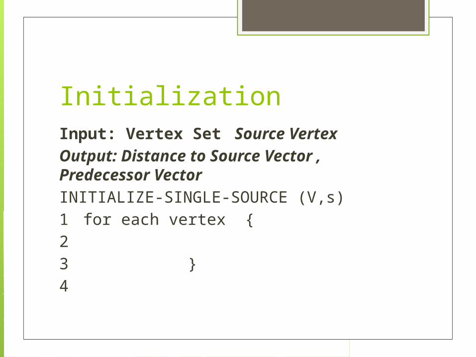
InitializationInput: Vertex Set Source Vertex Output: Distance to Source Vector , Predecessor Vector INITIALIZE-SINGLE-SOURCE (V,s)1 for each vertex {2 3 }4

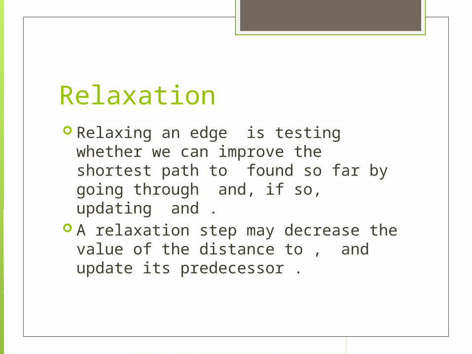
Relaxation Relaxing an edge is testing whether we

can improve the shortest path to found so far by going through and, if so, updating and .

A relaxation step may decrease the value of the distance to , and update its predecessor .

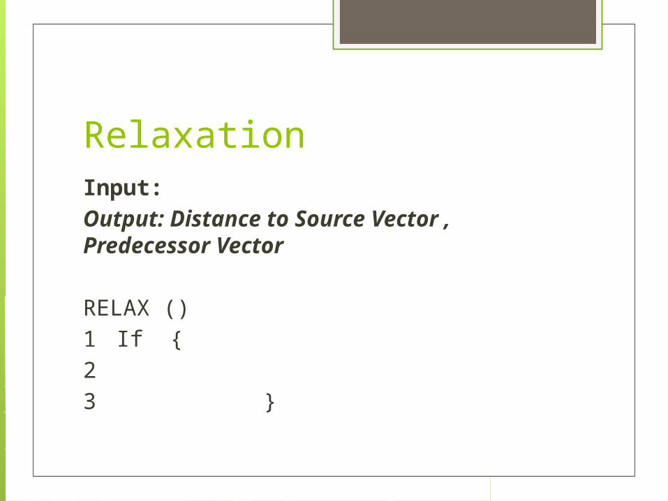
RelaxationInput: Output: Distance to Source Vector , Predecessor Vector

RELAX ()1 If {2 3 }

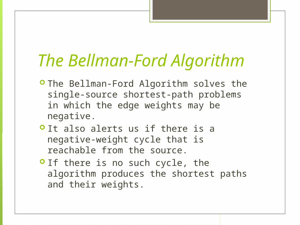
The Bellman-Ford Algorithm The Bellman-Ford Algorithm solves the

single-source shortest-path problems in which the edge weights may be negative.

It also alerts us if there is a negative-weight cycle that is reachable from the source.

If there is no such cycle, the algorithm produces the shortest paths and their weights.

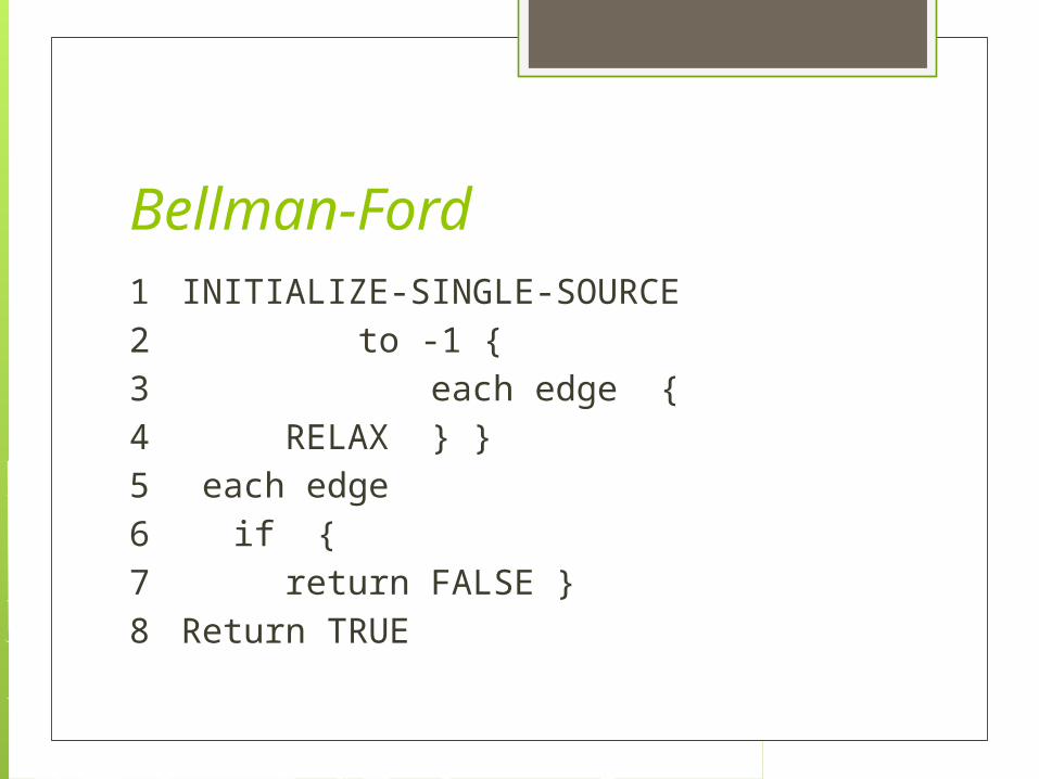
Bellman-Ford1 INITIALIZE-SINGLE-SOURCE 2 to -1 {3 each edge {4 RELAX } }5 each edge 6 if {7 return FALSE }8 Return TRUE

Example and Implementation Issues

Correctness Lemma:Let be a weighted, directed graph with source and weight function , and assume that contains no negative-cycles that are reachable from . Then, after -1 iterations of the for loop of lines 2-4 of BELLMAN-FORD, is the length of the shortest-path from to for each vertex reachable from .

Computational Complexity

O (|𝑉||𝐸|)

Dijkstra’s Algorithm Dijkstra’s algorithm solves the single-

source shortest-path problem on a weighted, directed graph in with nonnegative edge weights.

for each edge With a good implementation the running

time of Dijkstra’s algorithm is lower than that of Bellman-Ford algorithm.

Dijkstra’s Algorithm Dijkstra’s Algorithm maintains a set of

vertices whose final shortest-path distance from the source s have already been determined.

The algorithm repeatedly selects the vertex with the minimum shortest-path estimate, adds to , and relaxes all edges leaving .

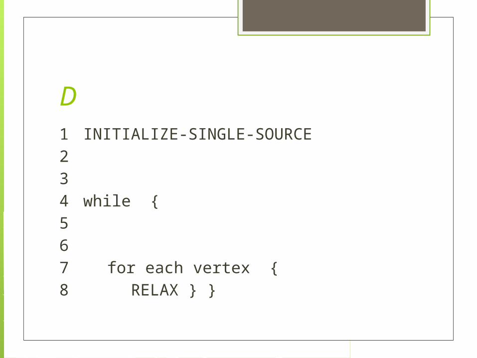
D1 INITIALIZE-SINGLE-SOURCE 2 3 4 while {567 for each vertex {8 RELAX } }

Example

Implementation Issues

Approach Because Dijkstra’s algorithm always

chooses the closest vertex in to add to the set , we say that it uses a “greedy” strategy.

Not all greedy strategies yield optimal results.

But in this case it does

Correctness Theorem: Dijkstra’s algorithm, run on a

weighted, directed graph with a nonnegative weight function terminates with a distance vector that consists of the shortest distances from the source to each vertex.

Proof: We use the following loop invariant: At the start of each iteration of the

while loop of lines 4-8, distance vector has the shortest distances for each vertex in . Initialization: trivially true Maintenance: Termination:

Computational Complexity The computational complexity of

Dijkstra’s algorithm depends on how is implemented.

By a Fibonacci heap implementation it is possible to obtain a running time of