Science of Computer

ELSEVIER Programming

Science of Computer Programming 22 (1994) 157-180

Shorter paths to graph algorithms

Bernhard Miiller*, Martin Russling

Institut fk Mathematik, Universitiit Augsburg, Uniwrsitiitsstr. 8, D-86135 Augsburg, Germany

Communicated by C. Morgan; revised October 1993

Abstract

We illustrate the use of formal languages and relations in compact formal derivations of some graph algorithms.

1. Introduction

The transformational or calculational approach to program development has by

now a long tradition (see [1,2,4,5,12]). In it, one starts from a (possibly nonexecutable)

specification and transforms it into a (hopefully efficient) program using semantics-

preserving rules. Many derivations, however, suffer from the use of lengthy expres-

sions involving formulae from predicate calculus. However, in particular in the case of

graph algorithms the calculus of formal languages and relations allows considerable

compactification. We use a simplified and straightened version of the framework

introduced in [14] to illustrate this with derivations of algorithms for computing the

length of a shortest path between two graph vertices and for cycle detection.

2. The framework

In connection with graph algorithms we use formal languages to describe sets of

paths. The letters of the underlying alphabet are interpreted as graph nodes. As

a special case of formal languages we consider relations of arities d 2. Relations of

arity 1 represent node sets, whereas binary relations represent edge sets. The only

two nullary relations (the singleton relation consisting just of the empty word and the

* Corresponding author. E-mail: {moeller,russling}@uni-augsburg.de.

0167-6423/94/%07.00 0 1994 Elsevier Science B.V. All rights reserved

SSDI 0167-6423(93)E0017-T

158 B. Miiller, M. Russling/ Science of Computer Programming 22 (1994) 157-180

empty relation) play the role of the Boolean values. This also allows easy definitions of

assertions, conditional, and guards.

Essential operations on languages are (besides union, intersection, and difference)

concatenation, composition, and join. As special cases of composition we obtain

image and inverse image as well as tests for intersection, emptiness, and membership.

The join corresponds to path concatenation on directed graphs; special cases yield

restriction.

Proofs are either straightforward or given by Moller [14] and therefore omitted.

2.1. Operations on sets

Given a set A we denote by B(A) its power-set. The cardinality of A is, as usual,

denoted by 1 Al. To save braces, we identify a singleton set with its only element.

Frequently, we will extend set-valued operations

f: Al x ... x A, -+ 9(A,+,) (n > 0)

to the powersets Y(Ai) of the Ai. In these cases we use the same symbolfalso for the

extended function

S: P(A,) x ... x g(A,) -+ g(A,+ I) >

defined by

fvJ1, . . . 3 U,) “2 u ... ,,J” fh, . . . > x,) x1eu1 n n

(1)

for Vi E Ai. By this definition, the extended operation distributes through union in all

arguments:

&NJ,, . . . > ui-1, (_) Uij, Ui+l,. 1. 2 Un) jeJ

=,~.f(“l~~. . 2 ui-l, Uij, ui+l,. . . > un).

By taking J = 0 we obtain strictness of the extended operation w.r.t. 0:

f(ul,. . .Y ui-l,O, ui+l>. . .T u*)=0.

By taking J = { 1,2) and using the equivalence

ucvouuv=v,

(2)

(3)

we also obtain monotonicity w.r.t. c in all arguments:

vi1 E vi* * f(“l, . . . 2 Ui-12 Uil, Ui+l, * . > un)

cft”l,. . . 7 UiG1, uiZ, Ui+l,. . . T un). (4)

Moreover, bilinear equational laws are preserved (see e.g. [ll]).

B. M6ller. M. Russtingl Science of Computer Programming 22 (1994) 157-180 159

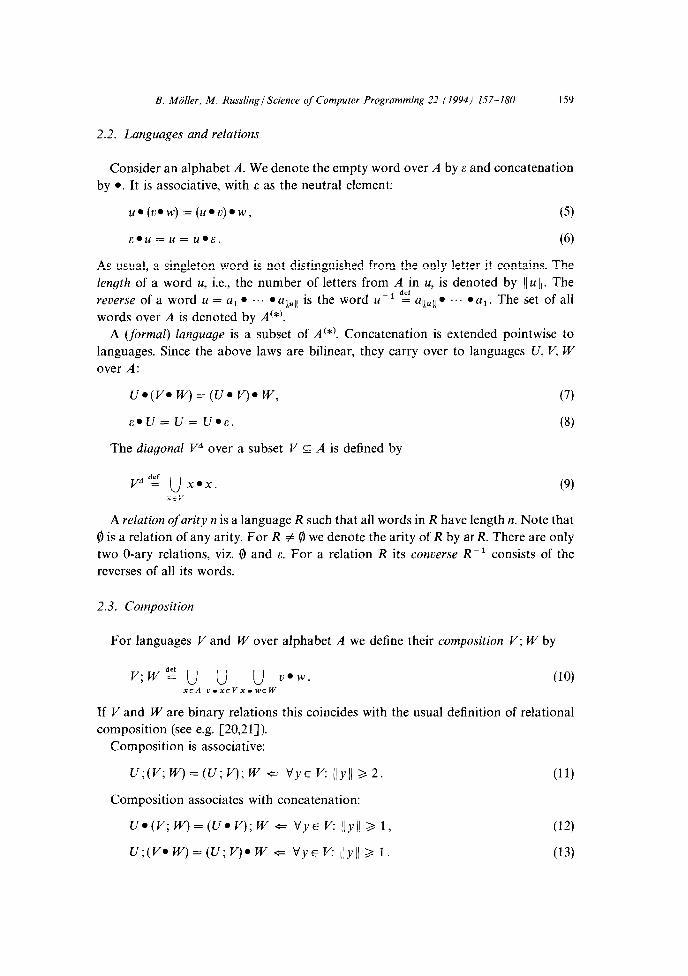
2.2. Languages and relations

Consider an alphabet A. We denote the empty word over A by E and concatenation

by 0. It is associative, with E as the neutral element:

U.(V.W) = (U.U).W, (5)

&Old = u = U@&. (6)

As usual, a singleton word is not distinguished from the only letter it contains. The

length of a word u, i.e., the number of letters from A in U, is denoted by J/uJl. The

reverse of a word u = a, l ... .allull is the word u-r “2’ %ll l ... l a,. The set of all

words over A is denoted by A(*).

A (formal) language is a subset of A (*). Concatenation is extended pointwise to

languages. Since the above laws are bilinear, they carry over to languages U, V, W

over A:

U.(V. W) = (U. V)e w,

amU= U= Ua&.

The diagonal Vd over a subset V G A is defined by

(7)

(8)

VA “2 u X.X. (9) XEV

A relation of arity n is a language R such that all words in R have length n. Note that

8 is a relation of any arity. For R # 8 we denote the arity of R by ar R. There are only

two 0-ary relations, viz. @ and E. For a relation R its converse R-l consists of the

reverses of all its words.

2.3. Composition

For languages V and W over alphabet A we define their composition V; W by

If V and Ware binary relations this coincides with the usual definition of relational

composition (see e.g. [20,21]).

Composition is associative:

U;(V; IV) = (U; V); w e vy+E J? [(yI( 3 2.

Composition associates with concatenation:

U.(V;W)=(U.V);W .S= VyEv: I/y/[ 21,

U;(V@W)=(U;V).W S= vyev: jlyj( 3 1.

(11)

(12)

(13)

160 B. Mbller, M. Russling J Science of Computer Programming 22 (1994) 157-180

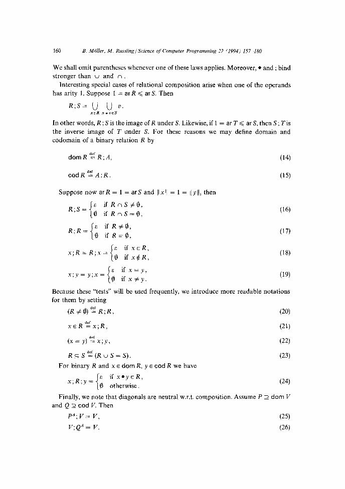
We shall omit parentheses whenever one of these laws applies. Moreover, l and ; bind stronger than u and n .

Interesting special cases of relational composition arise when one of the operands has arity 1. Suppose 1 = ar R < ar S. Then

R;S= u u v. xsR x.usS

In other words, R ; S is the image of R under S. Likewise, if 1 = ar T d ar S, then S ; T is the inverse image of codomain of a binary

domRd:R;A,

codRdz A;R.

T under S. For these reasons we may define domain and relation R by

Suppose now ar R = 1 = ar S and I/ x (I = 1 =

R’S= i

E if RnS#@,

8 if RnS=@,

R’R= F if R#@, fj ifR=lj$,

II Y IO then

(141

(15)

(16)

(171

Because these “tests” will be used frequently, we introduce more readable notations for them by setting

(R #@)“z R;R, (20)

xcRdLfx;R, (21)

(x=y)%;y, (22)

RrSdz(RuS=S). (23)

For binary R and x E dom R, y E cod R we have

x;R;y= E if x*ytzR,

8 otherwise. (24)

Finally, we note that diagonals are neutral w.r.t. composition. Assume P 2 dom V and Q -z cod I/. Then

P; V= V, (251

V;Q“ = V. (261

B. Mdler, M. RusslinglScience of Computer Programming 22 (1994) 157-180 161

2.4. Assertions

As we have just seen, the nullary relations E and 0 characterize the outcomes of

certain test operations. More generally, they can be used instead of Boolean values;

therefore, we call expressions yielding nullary relations assertions. Note that in this

view “false” and “undefined” both are represented by 8. Negation is defined by

$Z&-, (27)

fj “Af 0. (28)

Note that this operation is not monotonic.

For assertions B and C we have e.g. the properties

B*C=BnC, (29)

BOB= B, (30)

BOB= 0, (31)

Bu~?=F, (32)

B*C=BuC. (33)

Conjunction and disjunction of assertions are represented by their intersection and

union. To improve readability, we write B A C for B n C = B l C and B v C for

B u C. For assertion B and arbitrary language R we have

Hence, B l R (and R l B) behaves like the expression

B D R = if B then R else error fi

in [13]. We will use this construct for propagating assertions through recursions.

2.5. Conditional

Using assertions we can also define a conditional by

if B then R else S fi “2 B l R u Be S (35)

for assertion B and languages R and S. Note that this operation is not monotonic in B.

2.6. Join

A useful derived operation is provided by a special case of the join operation as used

in database theory (see e.g. [8]). Given two languages R and S, their join R WS

162 B. Mdler, M. Russlingj Science of Computer Programming 22 (1994) 157-180

consists of all words that arise from “glueing” together words from R and from

S along a common intermediate letter. By our previous considerations, the beginnings

of words ending with x E A are obtained as R; x, whereas the ends of words which

start with x are obtained as x ; S. Hence, we define

RwS “2 u R;x.x*x;S. XGA

(361

Again, w binds stronger than u and n. Join and composition are closely related. To explain this we consider two binary

relations R, S G A l A:

R;S= u {xay: x.z~Rr\z*y~S}, ZEA

RwS= u {x*zay: x*z~Rr\z*y~S}. ZEA

Thus, whereas R ; S just states whether there is a path from x to y via some point z E A, the relation R w S consists of exactly those paths x l z l y. In particular, the relations

R,

RwR,

Rw(RwR),

consist of the paths of edge numbers 1,2,3, . . . in the directed graph associated

with R. Other interesting special cases arise when the join is taken w.r.t. the minimum of the

arities involved. Suppose 1 = ar R < ar S. Then

RwS = u R;x@x.x;S = u x.x;S. XEA XGR

In other words, R w S is the restriction of S to R. Likewise, for T with 1 = ar T d ar S,

the language S w T is the corestriction of S to T. If even ar R = ar S = 1 we have

RwS=RnS.

In particular, if ar R = 1 and (1 x I( = 1 = II y II,

RwR=R,

(37)

x xwR=Rwx=

if xER,

8 if x$R,

i

x if x=y, xwy=ywx=

8 if x#y.

(38)

(39)

(40)

B. Miifler, M. Russlingj Science of Computer Programming 22 (1994) 157-180 163

For binary R, x E dom R and y E cod R, this implies

xwRwy= x.y if x*yeR,

8 otherwise. (41)

In special cases, the join can be expressed by a composition: assume arP =

1 = ar Q. Then

PwR = PA;R, (42)

RwQ=R;Q’. (43)

By the associativity of composition (11) also join and composition associate:

(RwS);T=Rw(S;T), (44)

R;(SwT)=(R;S)wT. (45)

provided ar S 3 2.

Moreover, also joins associate:

Rw(SwT)=(RwS)wT. (46)

2.7. Kleene algebras and closures

A Kleene algebra (see [7]) is a tuple (S, C, O,O, 1) consisting of a set S, operations

C: Y(S) -+ S and o : S l S + S and elements 0,l E S such that (S, 0, 1) is a monoid and

c(b=o,

C{x} = X (XES),

C( u X-) = Z{CK:K E X} (X- s B(S)), (47)

C(KoL) = (CK)O(CL) (KYLE 9(S)),

where in this latter equation o is the pointwise extension of the monoid operation.

Note that this implies that 0 is a zero with respect to 0 or, in other words, that 0 is

strict with respect to 0:

00x = 0 = x00. (48)

The binary version of C is

x+yd~Z{x,y}, (49)

which makes (S, +, 0) a commutative monoid. By our definitions, for an alphabet A,

LAN 2 (B(A’*‘),U,a,$,&),

REL 2 (Y(A.A),U,;,@,A’),

164 B. Mbller, M. Russlingl Science of Computer Programming 22 (1994) 157-180

all form Kleene algebras. Given a Kleene algebra one can define a partial order < by

clef xby 0 x+y=y. (50)

This makes (S, <) into a complete lattice. Moreover, o is continuous w.r.t. <. In our

examples < coincides with c . One can then define a closure operator .* by

x*d$y.l+xoy, (51)

where 1 is the least fixpoint operator. Using continuity we can represent the closure

also by Kleene’s approximation sequence (see [lo]) as

x* = C(xj: jE N}, (52)

where

xo d&f 1 3 (53)

xj+l “Lf xOxj. (54)

For our particular Kleene algebras we denote the closure operations by .(*), .*, and

. *, respectively.

Consider now a binary relation R E A. A and let G be the directed graph asso-

ciated with R, i.e., the graph with vertex set A and arcs between the vertices

corresponding to the pairs in R. We have, in REL,

” Ri’y =

E if there is a path with i edges from x to y in G,

0 otherwise. (55)

Hence,

x’R* ” =

E if there is a path from x to y in G,

8 otherwise. (56)

For S c A, the set S; R* gives all points in A reachable from points in S via paths in G,

whereas R*; S gives all points in A from which some point in S can be reached.

Finally,

S;R”;T= E if S and T are connected by some path in G,

8 otherwise. (57)

As usual, we set

R+ “2 R;R* = R*;R. (58)

Analogously, the path closure R * in PAT consists of all finite paths in G. Hence,

xwR’wy

is the language of all paths between x and y in G.

(59)

B. Miiller, M. Russlingl Science of Computer Programming 22 (1994) 157-180 165

Moving away from the graph view, the path closure is also useful for general binary

relations. Let e.g. d be a partial order. Then d * is the language of all <-

nondecreasing sequences. If < is even a linear order then <’ is the language of all

sequences which are sorted w.r.t. 6. This is exploited in [16,19] for the derivation of

sorting algorithms.

We now state some important induction principles for closures. We call a predicate

P over a Kleene algebra (S, Z;, o, 0,l) continuous if for all T E S

=z+ P[CT]. (60)

Lemma 2.1. Consider a jixed z E S and let P be continuous. lf P[l] and P[x] = P [z o x] or P[x] 3 P[x o z] then P[z*] holds as well.

Proof. A straightforward induction shows P[z’] for all i E N. Now Kleene’s approx-

imation (52) and continuity show the claim. 0

Corollary 2.2. Considerjxed U E Y(A(*‘), R c A l A and suppose that P is a continu- ous predicate on .Y(A(*)). If P[U] and P[ V] * P[ V; R] then P [U; R*] as well.

Proof. Define Q [X] over ??‘(A l A) by

Q[X] “g P[U;X].

Then Q satisfies the assumptions of Lemma 2.1 showing the claim. 0

A variant of the general induction principle of Lemma 2.1 allows us to extend

properties of x to x*.

Lemma 2.3. Let P be continuous and assume P[l] and P[x] A P [y] * P[x o y]. Then P[x] * P[x*] holds as well.

Proof. Analogous to the proof of Lemma 2.1. 0

We shall see various applications of these principles later on.

3. Graph algorithms

We now want to apply the framework in case studies of some simple graph

algorithms.

166 B. Mdler. M. Russling/ Science of Computer Programming 22 (1994) 157-180

3.1. Length of a shortest connecting path

3.1 .l. Specljication and first recursive solution We consider a finite set A of vertices and a binary relation R E A l A. The problem

is to find the length of a shortest path from a vertex x-to a vertex y. Therefore, we

define

shortestpath(x, y) “2 min(edgelengths(x w R” w y)) , (61)

where, for a set S of (nonempty) paths,

edgelengths “2 U ( (/ s )I - 1) SES

(62)

calculates the set of path lengths, i.e., the number of edges in each path, and, for a set

N of natural numbers.

def min(N) =

k if kENr\NEk;<, 8 if N = @. (63)

It is obvious that edgelengths is strict and distributes through union. Moreover, for

unary S,

edgelengths(Sw T) = 1 + edgelengths(S; T),

and, for M, N G fW,

(64)

min(M u N) = min(min(M) u min(N)), (65)

min(0 u M) = 0. (66)

For deriving a recursive version of shortestpath we generalize it to a function sp

which calculates the length of a shortest path from a set S of vertices to a vertex y:

sp(S, y) “2 min(edgelengths(S w R’w y)). (67)

The embedding

shortestpath(x, y) = sp(x, y)

is straightforward.

We calculate

SP(S, Y)

= {definition]

(68)

min(edgelengths(S w R’w y))

= @by (51)D

min(edgelengths(S w (A u R w R’) w y))

= {distributivity]

B. Mdler, M. RusslinglScience of Computer Programming 22 (1994) 157-180 167

min(edgeZengths(S w Aw y) u edgelengths(S w R w R’ w y))

= @by (37)D

min(edgelengths(S w y) u edgelengths(S w R w R’ w y)) .

By (39) the subexpression SW y can be simplified according to whether y E S or not.

Case 1: y E S.

min(edgelengths(S w y) u edgeZengths(S w R w R’ w y))

= {by (39), since y E SD

min(edgelengths(y) u edgelengths(S w R w R’ WY))

= {definition of edgelengths]

min(O u edgelengths(S w R w R’ w y))

= @by (WD

0.

Case 2: y$S.

min(edgelengths(S w y) u edgeZengths(S w R w R’ w y))

= {by (39), since y #SD

min(edgelengths(@) u edgelengths(S w R w R’ w y))

= {strictness, neutrality]

min(edgelengths(S w R w R’ w y))

= @by (640

min(1 + edgelengths(S; R w R’ w y))

= {distributivity]

1 + min(edgelengths(S; R w R’ w y))

= {definition)

1 + sp(S;Ry).

Altogether we have derived the recursion equation

sp(S, y) = if y E S then 0 else 1 + sp(S; R, y) fi. (69)

Note, however, that termination cannot be guaranteed for this recursion. To make

progress in that direction we show some additional properties of sp.

168 B. MBller, M. Russling J Science of Computer Programming 22 (1994) 157-180

Lemma 3.1. u T,y) = min(sp(S,y) u sp(T,y)).

Proof.

SP(S u T,Y)

= {definition]

min(edgelengths((S u T) w R’ w y))

= {distributivity]

min(edgelengths(S w R” w y) u edgelengths( T w R’ w y))

= @by (65)D

min(min(edgelengths(S w R’ w y)) u min(edgelengths(T w R’ w y)))

= {definition]

min(sp(S, Y) u sp(T, Y)). q

We now consider again the case y#S. From (69) we obtain

sp(S; R, Y) f sp(S, Y) >

and hence

(70)

sp(S, Y)

= {by y 4 S and (69))

1 + sp(S;R, y)

= @by (70)D

1 + mWsp(S, Y) u SP@; R, ~1)

= {by Lemma 3.1)

1 + sp(S u S; R,y).

so that a second recursion equation for sp is

sp(S,y)=ify~SthenOelse l+sp(SuS;R,y)fi. (71)

Now, although the first parameter is nondecreasing in each recursive call, still

nontermination is guaranteed if there is no path from S to y. However, in that case by

finiteness of A the recursive calls of sp eventually become stationary, i.e., eventually

S = S u S ; R holds, which is equivalent to S; R c S. We consider that case in the

following lemma.

Lemma 3.2. If y $ S and S; R G S then S w R’ w y = 0, i.e., there is no path from set S to vertex y, and therefore sp(S, y) = 8.

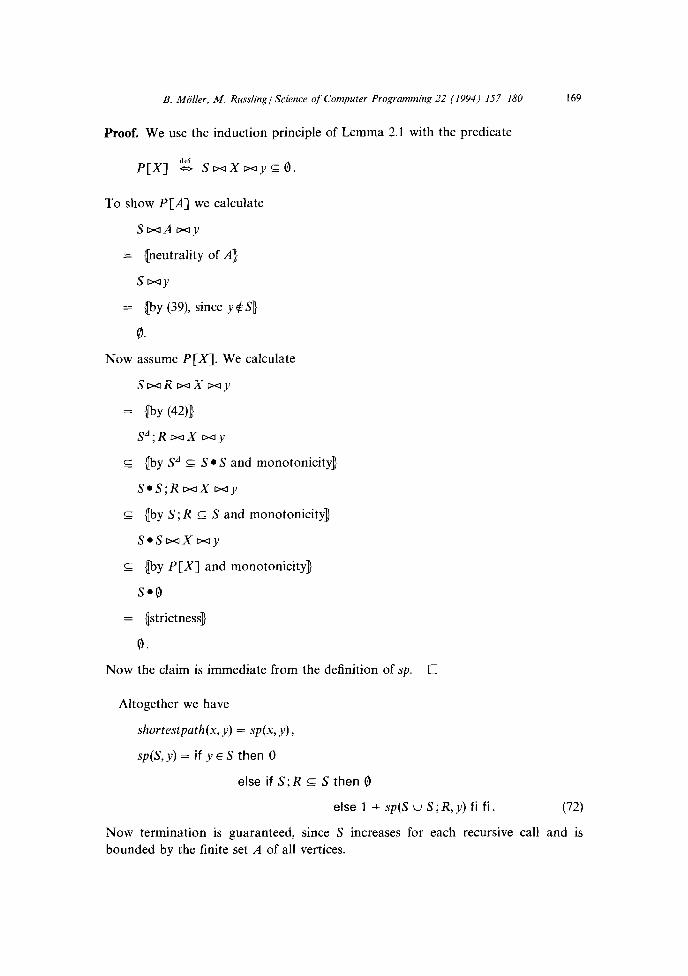
B. Miiller, M. Russlingj Science of Computer Programming 22 (1994) 157-180 169

Proof. We use the induction principle of Lemma 2.1 with the predicate

P[X] 2t swxDayc@.

To show P[A] we calculate

SwAwy

= {neutrality of Al

s WJ’

= {by (39), since y$ SD

8.

Now assume P[X]. We calculate

SwRwXwy

= eby (420

SA,RwXwy

c {by SA E S l S and monotonicityJ

S.S;RwXwy

_c {by S; R c S and monotonicityj

S.SwXDay

E {by P[X] and monotonicityJ

SOB

= @trictnessj

8.

Now the claim is immediate from the definition of sp. 0

Altogether we have

shortestpath(x. y) = sp(x, y) ,

sp(S, y) = if y E S then 0

else if S;R E S then 8

else 1 + sp(S u S;R,y)fi fi. (72)

Now termination is guaranteed, since S increases for each recursive call and is

bounded by the finite set A of all vertices.

170 B. Mdler. M. RusslinglScience of Computer Programming 22 (1994) 157-180

3.1.2. Improving eficiency One may argue that in the above version, accumulating vertices in the parameter

S is not efficient because it makes calculating S ; R more expensive. So, in an improved

version of the algorithm, we shall keep as few vertices as possible in the parameter

S and the set of vertices already visited in an additional parameter T, tied to S by an

assertion. Let

sp2(S,T,y)d~(SnT=@~y$T)*sp(Su T,y), (73)

with the embedding

shortestpath(x, y) = sp2(x, $, y).

Now assume S n T = 8 A y ef T. Again we distinguish two cases.

(74)

Case 1: y E S.

sp2(S, T, Y)

= {definition]

MS u T,Y)

= {by y E S c_ S u T and (72)]

0.

Case 2: y $ S.

sp2(S, T, Y)

= {definition)

SP(S u T,Y)

= {by y$S u Tand (72))

if (Su T);R ESU Tthen0

else1 +sp(Su Tu(Su T);R,y)fi

= {set theory]

if (Su T);R E Su Tthen0

else 1 + sp(((S u T); R)\(S u T) u (S u T),y)fi

= {definition and y C$ S u Tj

if (Su T);R CSU Tthen0

else1 + sp2(((S u T);R)\(S u T),S u T,y)fi.

B. Mdler, M. Russlingl Science of Computer Programming 22 (1994) 157-180 171

Altogether,

shortestpath(x, y) = sp2(x, 8, y) ,

sp2(S,T,y)=(SnT=0r\y$#T)*

ifyES

then 0

elseif(Su T);RzSu T

then 0

else1 + spZ(((S u T);R)\(S u T),S u T,y)fifi.

This version is still very inefficient. However, a simple analysis shows that the

assertion of sp2 can be strengthened by the conjunct T; R c S v T. Thus, one can

simplify the program to

shortestpath(x, y) = sp3(x, 0, y) ,

sp3(S,T,y)=(SnT=0r\y$Tr\T;R~SvT).

if YES

then 0

el.seifS;RcSu T

then 0

else1 + sp3((S;R)\(S u T),S u T,y)fifi.

The formal derivations steps for this are similar to the ones above and hence we omit

them.

Termination is guaranteed, since T increases for each recursive call and is bounded

by the finite set A of all vertices.

Note that a tail-recursive variant can easily be derived from sp3 by introducing an

accumulator. A corresponding algorithm in iterative form can be found in the

literature, e.g. in [9] (but there unfortunately not faultless).

Further, our algorithm also solves the problem whether a vertex y is reachable from

a vertex x, since

reachable(x, y) = (shortestpath(x, y) # 0). (75)

3.2. Cycle detection

3.2.1. Problem statement andfirst solution

Consider again a finite set A of vertices and a binary relation R c A l A. The

problem consists in determining whether R contains a cyclic path, i.e. a path in which

a node occurs twice.

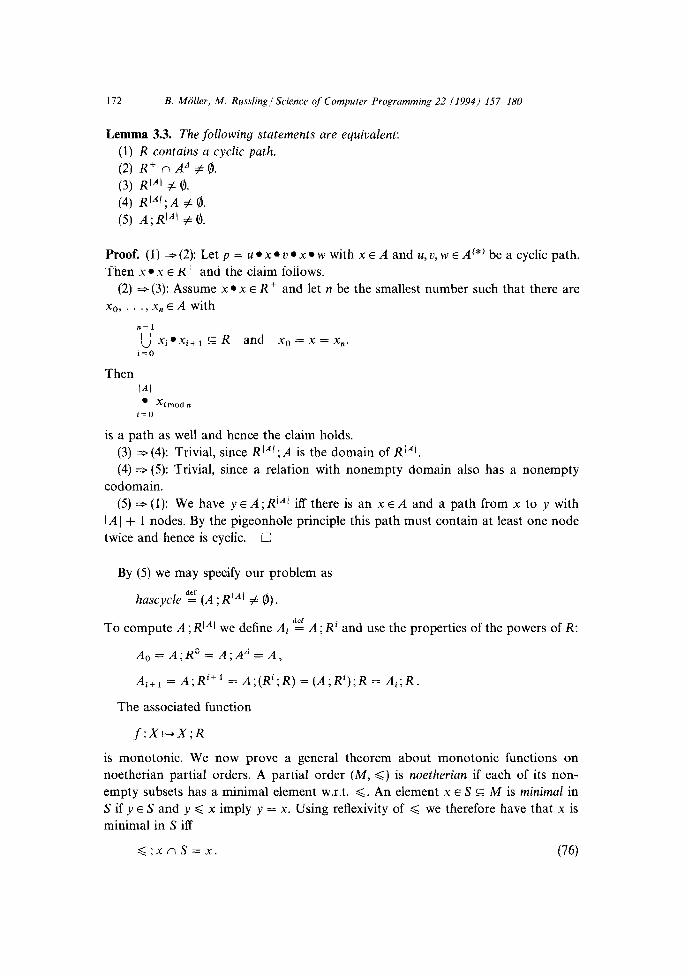
172 B. MBller, M. Russling/Science of Computer Programming 22 (1994) 157-180

Lemma 3.3. The following statements are equivalent:

(1) R contains a cyclic path.

(2) R+ n AA #8.

(3) RIA’ # 0.

(4) RIA’; A # 0.

(5) A; RIA’ # 0.

Proof. (1) =j (2): Let p = u l x l u l x l w with x E A and u, u, w E A(*) be a cyclic path.

Then x l x E R+ and the claim follows.

(2) 5 (3): Assume x l x E R+ and let n be the smallest number such that there are

x0, . .> x, E A with

n-1 i~oxi*xi+~GR and x0=x=x,.

Then IAl l Ximodn

i=O

is a path as well and hence the claim holds.

(3) q (4): Trivial, since RI”; A is the domain of RIAI.

(4) G- (5): Trivial, since a relation with nonempty domain also has a nonempty

codomain.

(5) * (1): We have y E A ; R IAl iff there is an x E A and a path from x to y with

(Al + 1 nodes. By the pigeonhole principle this path must contain at least one node

twice and hence is cyclic. q

By (5) we may specify our problem as

hascycle “2 (A; RIAl # 0).

To compute A ; RIAl we define Ai “g A; R’ and use the properties of the powers of R:

Ao=A;Ro=A;AA=A,

Ai+l = A;R’+’ = A;(R’;R) = (A;R’);R = Ai;R.

The associated function

f :XHX;R

is monotonic. We now prove a general theorem about monotonic functions on

noetherian partial orders. A partial order (M, <) is noetherian if each of its non-

empty subsets has a minimal element w.r.t. <. An element x E S E M is minimal in

S if y E S and y < x imply y = x. Using reflexivity of d we therefore have that x is

minimal in S iff

<;xnS=x. (76)

B. Mdler, M. Russling/Science of Computer Programming 22 (1994) 157-180 173

Viewing a function f : M 4 M as a binary relation, we can form its closuref *. Then,

for x E M, we have

x;f * = {fi(x): iEN}, (77)

where the fi are defined as usual.

Theorem 3.4. Let (M, <) be a noetherian partial order and f : M --f M a monotonic

total function.

(1) (2)

(3)

Iffor x E M we have f (x) d x then x, 2’ glb (x; f *) exists and is afixpoint off.

Assume x as in (1) and y E M with x, < y d x. Then also y, = glb(y; f *) exists

and y, =xm.

If M has a greatest element T then T, exists and is the greatest jixpoint off:

Proof. We first restate in relational notation some of the notions involved.

(a)jisatotalfunctioniffAdEf;fU1andf-’;fzAd.

(b) f is monotonic iff< ; f c f; <

(c) u < v is equivalent to both u z d ; v and v c u; d.

(d) By our convention about singleton sets, f(x) and x ; f are the same for a total

function f.

In particular, (a) implies, for S G M.

(S;f)” = f -‘;P;f. (78)

We now treat the claims in order.

(1) We first show that

VyEx;f*:f(y)< y. (79)

Relationally, this means (x ; f *)” E f; <. We use the induction principle from Corol-

lary 2.2 with the predicate

P[X] z Xdzf; <

and U = x, R = f. P[x] holds by assumption. To infer P[X; f ] from P[X] we

calculate

(X;_f)A

= IIby (78))

f -‘;XA;f

G {by P[X] and monotonicityj

f -‘if; G;f

G (Tf is a function, neutrality]

174 B. Mdler, M. Russling/ Science of Computer Programming 22 (1994) 157-180

G Qf monotonic]

f;<.

Since (M, <) is noetherian, x ; f * has a minimal element x, . For this we calculate

X,

= {by minimality (76)l

b;x, nx;f*

=, {by (79) and monotonicity of n]

x,;fnx;f*

= 4 sincex,;f E x;f*J

x,;f.

However, by totality off this means x, ; f = x, so that x, is a fixpoint off. We shall see below that x, = glb(x; f *).

(2) Using the induction principle from Lemma 2.3 it is immediate to show the

following facts:

X;fsX * X;f*EX, (80)

<;f sf;< * d;f* c f*;<, (81)

x;f s d;x =- x;f* E <;x. (82)

From (80) and X E X ; f * by Ad s f * we infer

X;fsX - X;f*=X. (83)

Now consider u, v E M with u d v. Then

U<V

0 {image]

vGu;<

* {monotonicity]

v;f* cu; d ;f*

* {f monotonic and (81))

v;f* G u;f*;B,

B. Miiller, M. Russlingl Science of Computer Programming 22 (1994) 157-180 17.5

so that u ;f* is a minorant for v ;f *. In particular, taking u = x, and v = x or v = y

and using (83) and (82) we see that x, is a lower bound for both y ; f* and x; f*. This

also implies X, = glb(x;f*). Moreover, y;f* is a minorant of x; f * so that every

lower bound z for y ; f * also is a lower bound for x ; f * and hence satisfies z d x, But

this shows x co = glb(y;f*) = Y,.

(3) Trivially,f(T) < T, and hence T, exists by (1). Let x be a fixpoint of5 By the

proof of (2) we know that T;f* c x;f* ; d = x ; < so that x is a lower bound for

T;f*. This implies x < glb(T;f*) = T,. 0

A similar theorem has been stated by Cai and Paige [6].

Corollary 3.5. If T, d x for some x E M then T, = x,.

Proof. By (2) of the above theorem. 0

To calculate x, we define a function inf by

inf (y) “2 (x m<y6X).X,,

which determines x, using an upper bound y. We have the embedding x, = inf (x). Now from the proof of the above theorem the following recursion is immediate:

inf(y) = (x, d y d x)0 if y = f (y) then y else inf (f (y)) fi.

This recursion terminates for every y satisfying f (y) < y, since monotonicity then also

shows f (f (y)) d f (y), so that in each recursive call the parameter decreases properly.

In particular, the call inf (x) terminates. This algorithm is an abstraction of many

iteration methods on finite sets.

We now return to the special case of cycle detection. By finiteness of A the partial

order (P(A), 5 ) is noetherian with greatest element A. Therefore, A, exists. More-

over, we have the following corollary.

Corollary 3.6. A, Al = A,.

Proof. The length of any properly descending chain in P(A) is at most (A( + 1. Hence,

we have AlAI+ = AlAl and thus AlAl = A,. 0

So we have reduced our task to checking whether A, # 8, i.e., whether inf (A) # 8.

For our special case the recursion for inf reads (omitting the trivial part W E A)

inf(W) = (A, s W)@

if W = W; R then W else inf (W; R) fi .

We want to improve this by avoiding the computation of W; R. By the above

considerations we may strengthen the assertion of inf by adding the conjunct

176 B. Mdler, M. Russling/Science of Computer Programming 22 (1994) 157-180

W; R E W. We define

SK(W) “2 W\(W;R).

This is the set of sources of W, i.e., the set of nodes in W which do not have

a predecessor in W.

Now, assuming W; R E W, we have W = W; R o SK(W) = 0 and W; R =

W\src( W) so that we can rewrite inf into

inf(W)=(A,~ Wr\W;Rs W).

if src( W) = 8 then W else inf( W\src( W)) fi .

This is an improvement in that src( W) usually will be small compared to W, moreover,

the computation of src( W) can be facilitated by a suitable representation of R. Plugging this into our original problem of cycle recognition we obtain

hascycle = hey(A) , (84)

where

hey(W) = (A, c WA W;R c W).

if src( W) = 0 then W # 0 else hcy( W\src(W))fi , (85)

which is one of the classical algorithms which works by successive removal of sources

(see e.g. [3]). Note that Lemma 3.3(4) suggests a dual specification to the one we have

used; replaying our development for it would lead to an algorithm that works by

successive removal of sinks.

3.2.2. Improving eficiency

We want to improve the computation of the sets src( W). We observe that

x E src( W)

= XE W\(W;R)

=XE Wr\x$W;R

=XE Wr\R;xn W=@

=XE Wr\(R;xn Wj=O.

So we define for W G A the relation in(W) by

x;in(W) “2 ]R;x n WJ. (86)

Hence, x; in( W) gives the indegree of x w.r.t. W and

src(W) = Wn in(W);O. (87)

In final implementation, in(W) will, of course, be realized by an array. We aim at an

incremental updating of in in the course of our algorithm. We calculate

B. Miiiler, M. RusslinglScience of Computer Programming 22 (1994) 157-180 177

x;in(W\src(W))

= {definition]

IR;x n (W\src(W)I

= {set theory)

I(R;x n W\sWVl

= Q(A\B( = (A( - IA n BID

j(R;x n W)l - IR;x n Wn PC(W)]

= {src( W) z PVJ

((R;x n W)l - IR;x n src(W)I

= {definition)

x; in(W) - x; in(src( W)).

For binary relationsf, g with the same domain and subsets of N as codomains and

arithmetic operator 2 we define f {g by

x;(Rg) “2 (x;f)<(x;g). (88)

Then

in( W\src( W)) = in(W) - in(src( W)).

For the computation of in we observe that

in(@) = 0,

(89)

(90)

where

x;o “Af 0.

Moreover, if S # 8 and q E S is arbitrary we have

x ; in(s)

= x; in(q u S\q)

(91)

=IR;xn(quS\q)l

= l(R;x n 4) u (R;x n S\q)l

= lR;x n q1+ IR;x n S\ql

= x; in(q) + x; in(S\q),

when

x;in(q) = if q;R;x then 1 else 0 fi. (92)

178 B. Mdler, M. Russling/ Science of Computer Programming 22 (1994) 157-180

Then

in(S) = in(q) + in(S\q). (93)

We forego a transformation of in into tail recursive form, since this is completely

standard using associativity of +.

Now we can administer the source sets more efficiently. We introduce additional

parameters for carrying along SYC( W) and in(W) and adjust these parameters by the

technique of finite differencing (see e.g. [18]). We set, for S c W c A and relation f,

hc( W, S,f) 2 (S = src( W) A f= in(W)) l hcy( W)), (94)

with the embedding

hcy( W) = hc( W, src( W), in(W)) .

Now

hc(W,S,f)

= {definition$

(95)

if src(W) = 0 then W # 0 else hcy(W\src(W))

= {assertionJ

if S = 0 then W # 8 else hcy(W\S)

= {embedding]

if S = $ then W # 8 else hc(W\S,src(W\S), in(W\S))

= {introducing auxiliaries]

if S=@then W#8

elselet T”z W\S

let g “2 in(T)

inhc(T,src(T),g)fi.

= {by (89) and (87))

if S=Othen W#0

else let T “2 W\S

let g d2f- in(S)

inhc(T, T n g;O,g) fi.

A final improvement would consist in merging the computation of g with that of

T n g ;O using the tupling strategy (see e.g. [18]).

B. Mbller, M. RusslinglScience of Computer Programming 22 (1994) 157-180 179

4. Conclusion

The calculus of formal languages and relations has proved to speed up derivations;

in particular, the way from “nonoperational” specifications involving the closures R* and R’ to first recursive solutions. However, also the tuning steps in improving the

recursions have benefitted from the quantifier-free notation. If the resulting deriv-

ations still appear lengthy, this is to a great deal due to the fact that the assertions have

been constructed in a stepwise fashion (for mastering complexity) rather than in one

blow. Further case studies which demonstrate the viability of the approach in more

complicated examples are under way. Moreover, the framework has been applied to

other problem areas as well (see [l&17]).

Currently, we are working the definition of a more general program development

language based on this approach. While other authors use a purely relational

approach employing mostly even only binary relations, we find that relations with

their fixed arity are too unflexible and lead to a lot of unnecessary encoding and

decoding.

Acknowledgement

We are grateful to H. Partsch and to anonymous referees for a number of valuable

remarks.

References

VI

c21

c31

141

CSI

C61

c71 PI c91

Cl01 Cl11

F.L. Bauer, R. Berghammer, M. Broy, W. Dosch, F. Geiselbrechtinger, R. Gnatz, E. Hangel, W. Hesse,

B. Krieg-Briickner, A. Laut. T.A. Matzner, B. Mailer, F. Nick], H. Partsch, P. Pepper, K. Samelson,

M. Wirsing and H. Wiissner, The Munich Project CIP, Volume I: The Wide Spectrum Language CIP-L, Lecture Notes in Computer Science 183 (Springer, Berlin, 1985).

F.L. Bauer, B. Miiller, H. Partsch and P. Pepper, Formal program construction by transforma-

tions+omputer-aided, intuition-guided programming, IEEE Trans. Software Engrg. 15 (1989) 165-180. R. Berghammer, A transformational development of several algorithms for testing the existence of

cycles in a directed graph, Institut fiir Informatik der TU Miinchen, TUM-18615, Miinchen (1986).

R.S. Bird, Lectures on constructive functional programming, in: M. Broy, ed., Constructive Methods in Computing Science, NATO ASI Series Series F 55 (Springer, Berlin, 1989) 151-216.

R.M. Burstall and J. Darlington, A transformation system for developing recursive programs, J. ACM 24 (1977) 44-67.

J. Cai and R. Paige, Program derivation by fixed point computation, Sci. Comput. Programming 11

(1989) 197-261.

J.H. Conway, Regular Algebra and Finite Machines (Chapman and Hall, London, 1971).

C.J. Date, An Introduction to Database Systems, Vol. I (Addison-Wesley, Reading, MA, 4th ed., 1988).

M. Gondran and M. Minoux, Graphes et Algorithmes (Eyrolles, Paris, 1979). S.C. Kleene, Introduction to Metamathematics (Van Nostrand, New York, 1952).

P. Lescanne, Modeles non dtterministes de types abstraits, R.A.Z.R.O. Inform. Thkor. 16 (1982) 225-244.

180 B. Miiller, M. Russlingl Science of Computer Programming 22 (1994) 157-180

[12] L.G.L.T. Meertens, Algorithmics-towards programming as a mathematical activity, in: J.W. de

Bakker et al., eds., Proceedings CWI Symposium on Mathematics and Computer Science, CWI

Monographs 1 (North-Holland, Amsterdam, 1986) 289-334.

[13] B. Miiller, Applicative assertions, in: J.L.A. van de Snepscheut ed., Mathematics ofProgram Construc- tion, Lecture Notes in Computer Science 375 (Springer, Berlin, 1989) 3488362.

[14] B. Miiller, Relations as a program development language, in: B. Moller, ed., Constructing Programs from Specifications, Proceedings IFIP TC2J WG 2.1 Working Conference on Constructing Programs from Specifications, Pacijc Grove, CA, USA, 13-16 May 1991 (North-Holland, Amsterdam, 1991)

313-391.

[lS] B. Miiller, Towards pointer algebra, Sci. Comput. Programming 21 (1993) 57-90. [16] B. Miiller, Algebraic calculation of graph and sorting algorithms, in: D. Bjorner, M. Broy and I.V.

Pottosin, eds., Formal Methods in Programming and their Applications, Lecture Notes in Computer

Science 735 (Springer, Berlin, 1993) 394-413.

[17] B. Miiller, Derivation of graph and pointer algorithms, in: B. Moller, H.A. Partsch and S.A. Schuman,

eds., Formal Program Development, Lecture Notes in Computer Science 755 (Springer, Berlin, 1993)

123-l 60.

[lS] H.A. Partsch, Specification and Transformation of Programs-A Formal Approach to Software Deuel-

opment (Springer, Berlin, 1990).

[19] M. Russling, Hamiltonian sorting, Institut fur Mathematik der Universitlt Augsburg, Report No. 270

(1992). [20] G. Schmidt and T. Striihlein, Relations and Graphs, Discrete Mathematics for Computer Scientists,

EATCS Monographs on Theoretical Computer Science (Springer, Berlin, 1993).

[21] A. Tarski, On the calculus of relations, .I. Symbolic Logic 6 (1941) 73389.