NBER WORKING PAPER SERIES

SHORT-TERM, LONG-TERM, AND CONTINUING CONTRACTS

Maija Halonen-AkatwijukaOliver Hart

Working Paper 21005http://www.nber.org/papers/w21005

NATIONAL BUREAU OF ECONOMIC RESEARCH1050 Massachusetts Avenue

Cambridge, MA 02138March 2015

We would like to thank Oren Bar-Gill, Lucian Bebchuk, Kirill Borusyak, Donald Franklin, Louis Kaplow,Jeffrey Picel, Robert Scott, Kathryn Spier, Paul Tucker, Massimiliano Vatiero, and Luigi Zingalesfor helpful discussions. We have also benefitted from the responses of audiences at the 2014 FOMmeetings at the University of Southern California, at the University of Lausanne, and at Harvard LawSchool. We gratefully acknowledge financial support from the U.S. National Science Foundation throughthe National Bureau of Economic Research. The views expressed herein are those of the authors anddo not necessarily reflect the views of the National Bureau of Economic Research.

NBER working papers are circulated for discussion and comment purposes. They have not been peer-reviewed or been subject to the review by the NBER Board of Directors that accompanies officialNBER publications.

© 2015 by Maija Halonen-Akatwijuka and Oliver Hart. All rights reserved. Short sections of text,not to exceed two paragraphs, may be quoted without explicit permission provided that full credit,including © notice, is given to the source.

Short-term, Long-term, and Continuing ContractsMaija Halonen-Akatwijuka and Oliver HartNBER Working Paper No. 21005March 2015JEL No. D23,D86,K12

ABSTRACT

Parties often regulate their relationships through “continuing” contracts that are neither long-termnor short-term but usually roll over. We study the trade-off between long-term, short-term, and continuingcontracts in a two period model where gains from trade exist in the first period, and may or may notexist in the second period. A long-term contract that mandates trade in both periods is disadvantageoussince renegotiation is required if there are no gains from trade in the second period. A short-term contractis disadvantageous since a new contract must be negotiated if gains from trade exist in the secondperiod. A continuing contract can be better. In a continuing contract there is no obligation to tradein the second period but if there are gains from trade the parties will bargain “in good faith” usingthe first period contract as a reference point. This can reduce the cost of negotiating the next contract.Continuing contracts are not a panacea, however, since good faith bargaining may preclude the useof outside options in the bargaining process and as a result parties will sometimes fail to trade whenthis is efficient.

Maija Halonen-AkatwijukaDepartment of EconomicsSchool of Economics, Finance and ManagementUniversity of Bristol12 Priory RoadBristol BS8 1TNUnited KingdomMaija.Halonen@bristol.ac.uk

Oliver HartDepartment of EconomicsLittauer Center 220Harvard UniversityCambridge, MA 02138and NBERohart@harvard.edu

1. Introduction

A large literature in economics and law has studied why parties write long-term contracts. A leading explanation is that such contracts are useful to support specific investments, and there is much empirical support for this1. In a way it has been more challenging for economists to explain why parties write short-term contracts, that is, contracts that are shorter than the likely term of their relationship. The conventional answer is that it is costly for the parties to anticipate the contingencies that will arise during the latter part of their relationship and to write down unambiguously how to deal with them. However, as Maskin and Tirole (1999) have shown, if parties are fully rational, ingenious mechanisms can be used to get the parties to reveal information as their relationship progresses, and to incorporate this information into an enforceable contract. If there is even a reasonable chance that the parties’ relationship will endure it is hard to see why, under classical assumptions, such mechanisms would not be used. Thus the question remains: why do parties write short-term contracts?

The purpose of this paper is to investigate this question and in doing so also to study another question that as far as we know has received little attention from economists or lawyers. Why do parties often regulate their relationships through contracts that are neither explicitly long-term nor short-term, but rather are of indefinite duration in the sense that most of the time they roll over? Leading examples are rental contracts where the lease is typically renewed; month to month rental contracts with no lease; employment contracts where each party can (under some conditions) terminate the relationship, but where they usually do not – most of the time business continues “as usual”. We call such contracts “continuing”, although other terms are surely possible2.

Before proceeding we should make it clear that we do not view continuing contracts as necessarily legally enforceable. A tenant is typically not obliged to renew the lease or even to attempt to do so, and the landlord may have no such requirement either. Similarly, in many employment contracts, a worker can quit or a firm can fire the worker. Also, in a continuing relationship, the existence of a prior contract may put no legal constraints on how the parties negotiate the next contract3. In this paper we will be interested less in what is legally required than in how people actually behave. We will focus on the idea that the parties are likely to apply notions of fairness, fair dealing and good faith when they renegotiate continuing contracts even if they are not legally required to do so. Moreover, the prior contract is likely to be a very important reference point for determining whether a renegotiation is seen as fair4. For

1 See Williamson (1975) and Klein et al. (1978). For empirical evidence, see Goldberg and Erickson (1987), Joskow (1987), Crocker and Masten (1988), Pirrong (1993), Brickley et al. (2006), and Bandiera (2007). 2 We do not describe them as “indefinite-term contracts” since lawyers already use the term indefinite to describe preliminary agreements that may not be enforceable. See Bebchuk and Ben-Shahar (2001) and Schwartz and Scott (2007) for an analysis of such agreements. 3 But in some cases the parties may have an obligation to bargain in good faith. See Schwartz and Scott (2007). 4 Kahneman et al. (1986), a paper to which we return below, provides considerable support for the idea that past transactions serve as a reference point for future ones. See also Okun (1981). Rotemberg (2011) analyzes the optimal pricing policy for a firm that faces consumers who can be antagonized by prices that are higher than usual. Bar-Gill and Ben-Shahar (2003) argue that fairness is an important consideration when contracts are renegotiated and that previously agreed-upon terms will influence what is regarded as fair.

2

example, consider a new rent or wage. Whether this is regarded as reasonable or not will be judged in light of the initial rent or wage: attention will be focused on the change. Of course, other factors can be important, such as market conditions, but the prior terms that the parties agreed to will have particular salience5. We will be interested in analyzing the consequences of this for the choice of an optimal contract. We will argue that using the prior contract as a reference point can have costs as well as benefits. On the one hand it can mean that there is less to argue about if not much has changed in the relationship. On the other hand, it may make it more difficult to take certain kinds of outside options into account, which may cause inefficiency.

We will consider a situation where parties have a choice between a long-term, a short-term, and a continuing contract. A short-term contract is one where the parties agree in advance that they will not be bound by considerations of fairness or good faith if they negotiate a future contract. A continuing contract is one where the parties agree that they will be bound by such considerations6. Of course, in practice the choice may not be as clear-cut as this. For example, one of the authors of this paper has rented a vacation house for many years in a row. The relationship as it has developed is best thought of as continuing even though no language was ever used to that effect. This is a situation where a short-term contract was probably feasible only if one or both parties had no intention of renewing. Nonetheless it is useful to consider the choice of all three contracts—long-term, short-term, continuing --since economists have traditionally focused on long-term and short-term contracts. We will return to this issue of feasibility in the conclusions7.

To analyze continuing contracts, we apply the contracts as reference points approach developed in Hart and Moore (2008). According to this approach one role of a contract is to get parties “on the same page”, so as to avoid future misunderstanding. Misunderstanding leads to aggrievement and shading (in the form of departures from consummate performance), and consequent deadweight losses. Hart and Moore (2008) show that, under these conditions, Maskin-Tirole-type mechanisms lose their force and

5 Some support for the idea that prior transactions serve as a reference point can also be found in the law. The Uniform Commercial Code, Article 2-305, deals with the case where parties have signed a contract but left the price open. Subsection 2, dealing with the case where the price is to be fixed by one party, includes the qualification that the price must be fixed in good faith. The commentary goes on to argue that ‘ in the normal case a “posted price” or a future seller’s or buyer’s “given price,” “price in effect,” “market price,” or the like satisfies the good faith requirement.’ (Italics added.) See Uniform Commercial Code 50 2014-2015. 6 Parties do sometimes include language in contracts about future negotiation. For example, Goldberg and Erickson (1987, footnote 29) describe a contract that was for three successive three-year terms. The contract stated that the parties could not terminate solely because the price was unsatisfactory without first engaging in good faith negotiation on the price. 7 It is worth noting that Kahneman et al. (1986) find that past transactions do not form a reference point if the previous transaction was explicitly temporary, supporting the distinction we make between short-term and continuing contracts. Also Bewley (1999) finds that while wages in the primary sector (long-term employment) are downward rigid, wages in the secondary sector (short-term positions) are flexible downward, again supporting our distinction between short-term and continuing contracts.

3

simple contracts can be optimal8. So far the contracts as reference points approach has been used to study situations where the current contract is a reference point for contractual revision or renegotiation. We adapt this approach to allow for the prior contract to be a reference point.

We consider a very simple model where a buyer and a seller can trade zero or one widgets in each of two periods. Both parties are risk neutral, there are no non-contractible investments, and there are no wealth constraints. It is known that trade is efficient in the first period. If trade is always efficient in the second period a long-term contract mandating trade in both periods (specific performance) is optimal. If trade is always inefficient in the second period a short-term contract specifying trade in the first period is optimal. But suppose that there is uncertainty about whether there are gains from trade in the second period. In this case neither a long-term contract nor a short-term contract achieves the first-best. A long-term contract can be renegotiated if it is learned that trade is inefficient at the beginning of the second period, but since the parties will argue about how to divide the gains from renegotiation this is costly. (Throughout we will assume that argument is costly because it leads to aggrievement and shading.) In the case of a short-term contract, if trade is efficient in the second period, the parties must negotiate a new contract from scratch and this is costly because the parties will argue about how to divide the gains from trade.

A continuing contract may be a good compromise. To emphasize, a continuing contract is one where there is no obligation to trade in the second period but if there are gains from trade the parties will bargain using the first period contract as a reference point. At the risk of an abuse of language we will sometimes refer to this as bargaining in good faith9. Using the first period contract as a reference point can reduce negotiation costs since there is less to argue about. For example, suppose that in the first period the buyer’s value of trade is 20, the seller’s cost is 10 and the price is 15. At the beginning of the second period the parties learn that the buyer’s second period value has increased to 24 and the seller’s second period cost is still 10; that is, surplus has increased by 4. Using the first period contract as a reference point means that argument will be confined to how the additional surplus of 4 will be split. This means that the new price will lie between 15 (the buyer gets all the incremental surplus) and 19 (the seller gets all the incremental surplus). In contrast if the parties bargain from scratch, as in a short-term contract, the argument will be over how to divide the surplus of 14: the price can be anywhere between 10 and 24.

Although the use of the prior contract as a reference point can reduce argument/bargaining costs and increase efficiency, this may not always be the case10. Consider the same situation as above, but suppose now that the seller has an outside option equal to 11 in period 2. We will argue that good faith

8 For some experimental evidence in support of the Hart-Moore theory, see Fehr et al. (2011), (2015). For some related field evidence, see Iyer and Schoar (2013). 9 Bargaining in good faith is not a well-defined concept in the law. It can sometimes mean as little as that the parties are willing to meet each other. However, it sometimes appears to mean considerably more. See Summers (1982) for a general discussion of good faith in contracts. 10 Hart and Moore (2008, Section V) consider the case where other parties’ contemporaneous contracts, as opposed to the buyer’s and seller’s own prior contract, are reference points for the current transaction. This can also be beneficial or costly depending on the circumstances.

4

may preclude this outside option from being used in the bargaining process. If the seller argues that she should be paid at least 21 in the second period this may be regarded as opportunistic or coercive since it cannot be justified on the basis of changes in value and cost within the relationship: it is not in the [15,19] range. Either the seller feels uncomfortable suggesting a price of 21 or the buyer is unwilling to go along with it; or, if it were to happen, B’s aggrievement and shading would be so great that the seller would be worse off accepting the new terms than if she simply quit and took her outside option. The result may be that the relationship ends and the seller takes her outside option even though this is inefficient.

We do not wish to argue that outside options can never be taken into account in the bargaining process. Whether they can or cannot will depend on the circumstances. In an influential study, Kahneman et al. (1986), using telephone surveys, posed hypothetical situations to people to elicit their standards of fairness. They found that people think that it can be fair for a firm to raise prices when its costs go up or to lower wages if it is losing money, but not fair for it to raise prices if its product becomes scarce or to lower wages if other workers are willing to work for less11. This is very supportive of our assumption that using changes in value or cost within the relationship to justify a price change is consistent with good faith bargaining whereas using outside options is not. At the same time Kahneman et al. suggest that appealing to outside options may be more acceptable if these outside options represent general market trends12. As they put it (p.730), “Some people will consider it unfair for a firm not to raise its wages when competitors are raising theirs. On the other hand, price increases that are not justified by increasing costs are judged less objectionable when competitors have led the way.” We will therefore also consider the case where outside options can be used in bargaining13. By this we simply mean that in the above example the buyer will be willing to pay 21 to keep the seller in the relationship if the seller’s outside option is 1114.

11 This is consistent with the arguments of Okun (1981). Okun emphasizes the importance of fairness in determining firms’ pricing decisions in what he calls “customer markets” (see Okun, p.154). He distinguishes between price increases based on cost increases, which are generally accepted as fair, and those based on demand increases, which are generally regarded as unfair (see Okun, p.170). 12 On this point see also http://www.npr.org/blogs/money/2014/02/07/273060341/episode-516-why-paying-192-for-a-5-mile-car-ride-may-be-rational . This podcast discusses whether Uber’s strategy of surge pricing is fair, with the conclusion being that while this might be the case if the increase in price is linked to general market conditions it would not be so if the price increase depended on the characteristics of individual customers. 13 This case is, of course, very familiar to academic economists: an employee gets an outside offer and asks his or her employer to respond and the employer does. But whether such behavior occurs, or is acceptable, can vary over time and with the industry or sector or country concerned. For example, in the case of academic economists responding to outside options has been common in the U.S. for a long time, but was uncommon in the U.K. until fairly recently. For a dynamic analysis of the path of wages in a world where employers match outside options, see Harris and Holmstrom (1982). 14Note that, even if it is difficult or costly to use outside options in bargaining, alternative arrangements may be possible that substitute for this. For example, Weitzman (1984) and Oyer (2004) argue that firms may index wages to profit or share prices as a way to avoid inefficient quits or lay-offs. Our model assumes that verifiable variables that can form the basis of an index do not exist, although we return to the possibility of indexation in the conclusions.

5

However, one of the implications of our analysis that should be stressed is that, to the extent that outside options cannot be used in bargaining, fairness or good faith has costs as well as benefits, and that ex post inefficient allocations will sometimes occur in an optimal (continuing) contract15.

We should note a distinction between continuing contracts and another type of contract that is observed in practice: a renewable contract. A renewable contract is one that continues if both parties agree. However, the terms under which the contract will be renewed are typically specified in advance: they may be the same as the terms of the initial contract, or they may be the terms that one of the parties is offering new contractors16. In contrast, we are interested in cases where the terms of the new contract are left open and can be adjusted according to new events (a worker’s wage may stay the same most of the time but every so often he or she will get a raise; rents will typically change at the end of a lease, etc.). We will show that under some conditions a continuing contract is superior to a renewable contract.

There is a large theoretical literature on the determinants of contract length, and we can mention only a few contributions. Some papers assume a fixed cost of writing a (possibly contingent) contract and derive contract length as a function of the volatility of the environment; see, e.g., Gray (1978) and Dye (1985). Harris and Holmstrom (1987) consider actual duration in a model where new information arrives but as they recognize there is no reason why the initial contract should not have infinite duration. Diamond (1991) argues that short-term contracts might be used by some borrowers to signal that they are of high quality and are willing to expose themselves to the hazards of renegotiation; he does not consider continuing contracts. MacLeod and Malcomson (1993), Che and Hausch (1999), and Segal (1999) identify situations where “no contract” achieves as good an outcome as a sophisticated (incomplete) contract, which can be interpreted as saying that long-term contracts are sometimes not needed; however, they also do not explain why continuing contracts are used.

Finally, Guriev and Kvasov (2005) consider a situation where a seller makes a relationship specific investment and a buyer and seller can trade continuously over time. The buyer has an outside opportunity whose arrival time is stochastic; if it arrives it is efficient for the relationship to terminate. They show that it is optimal for parties to write what they call an evergreen contract – an indefinite contract which can be terminated by the buyer (at some cost) with notice. However, they do not consider what we have called continuing contracts where future terms are left open.

The paper is organized as follows. In Section 2 we present the model and analyze the trade-off between long-term, short-term, and continuing contracts for the case of no outside options. In Section 3 we bring in outside options and consider both the case where they can be used in bargaining and the case

15 Herweg and Schmidt (2015) have also shown that inefficient allocations can arise when contracts are reference points if parties are loss-averse. They are concerned with a one period model where renegotiation takes place and do not study how a contract can be a reference point for transactions in future periods. 16 See Lafontaine and Shaw (1999). They note that when franchisees’ contracts are renewed this is usually done at the “then-current” contract terms. Masten (2009) provides evidence on the value of long-term, renewable contracts for the case of heterogeneous freight transactions.

6

where they cannot. In Section 4 we extend the analysis to other sorts of contracts, in particular, renewable and exclusive contracts. Finally, Section 5 concludes.

2. The Model

We consider a buyer B and a seller S engaged in a two period, three date relationship. See Figure 1 for a time-line. In each period they can trade zero or one widgets.

At date 0, B and S sign an initial contract that may be long-term, short-term, or continuing. This contract is negotiated under competitive conditions at date 0 in the sense that there are many alternative sellers for B and so each seller receives her outside option for the two periods, which we denote by 𝑢𝑢�. (One can imagine that B auctions off the initial contract to the potential sellers.) If the contract is long-term, it may be renegotiated at date 1. If the contract is short-term or continuing, a new contract between B and S may be negotiated at date 1 for the second period.

B’s value 𝑣𝑣1 and S’s cost 𝑐𝑐1 for the widget in period 1 are already known when the initial contract is written. We assume 𝑣𝑣1 > 𝑐𝑐1. At date 1, before the initial contract is renegotiated or a new contract is signed, B’s value 𝑣𝑣2, S’s cost 𝑐𝑐2, B’s outside option 𝑟𝑟𝐵𝐵, and S’s outside option 𝑟𝑟𝑆𝑆 for period 2 are observed by both parties – there is symmetric information throughout (but 𝑣𝑣2, 𝑐𝑐2, 𝑟𝑟𝐵𝐵 and 𝑟𝑟𝑆𝑆 are not verifiable)17. Trade in period 2 is efficient if and only if 𝑣𝑣2 − 𝑐𝑐2 > 𝑟𝑟𝐵𝐵 + 𝑟𝑟𝑆𝑆. At date 0, however, 𝑣𝑣2, 𝑐𝑐2, 𝑟𝑟𝐵𝐵 and 𝑟𝑟𝑆𝑆 are uncertain – they are drawn from a probability distribution 𝐹𝐹 (which is common knowledge). Both parties are risk neutral, there are no wealth constraints, and without loss of generality we suppose no discounting. We assume that 𝑢𝑢� is in a range where the buyer wants to offer the seller a contract18.

17 If 𝑣𝑣2, 𝑐𝑐2, 𝑟𝑟𝐵𝐵 and 𝑟𝑟𝑆𝑆 were verifiable contingent contracts could be written and the problems that we study in this paper would not arise. We discuss the observability-verifiability distinction further below. 18 We do not model the market for buyers and sellers at date 1. This would require a general equilibrium analysis in which there are several buyers and sellers at both dates 0 and 1 and the availability of alternative partners at date 1 depends on contracts signed at date 0. The outside options 𝑟𝑟𝐵𝐵 and 𝑟𝑟𝑆𝑆 are a crude and short-cut way of representing market alternatives at date 1. We also do not model why the market is more competitive at date 0 than at date 1. In the background there may be some relationship-specific investments or other types of lock-in. Note, however, that the existence and extent of lock-in is captured implicitly. If 𝑣𝑣2 − 𝑐𝑐2 > 𝑟𝑟𝐵𝐵 + 𝑟𝑟𝑆𝑆 with high

7

For simplicity we assume that B has all the bargaining power in any negotiation or renegotiation at date 1.

Although bargaining at date 1 occurs under symmetric information it is not costless. We suppose that the parties have different feelings of entitlement concerning their payoff from bargaining and since at least one of them will be disappointed this leads to aggrievement and shading and consequently deadweight losses. We will explain the details of this below.

It is convenient to focus in this section on the case where there are no outside options at date 1 – 𝑟𝑟𝐵𝐵 ≡ 𝑟𝑟𝑆𝑆 ≡ 0. We introduce outside options in Section 3.

Long-term contract

Suppose first that the parties write a long-term contract at date 0, specifying trade in both periods (a specific performance contract). Without loss of generality we can assume the same price in each period, which we denote 𝑝𝑝. At date 1 the parties will learn 𝑣𝑣2 and 𝑐𝑐2. Obviously, if 𝑣𝑣2 > 𝑐𝑐2there are no gains from renegotiation. However, if 𝑣𝑣2 < 𝑐𝑐2, B and S will want to renegotiate19.

Recall that we assume that B has all the bargaining power. Thus B will offer S an amount (𝑝𝑝 − 𝑐𝑐2) – her second period payoff under the existing contract – in return for not trading. However, following Hart and Moore (2008), we suppose that S feels entitled to more of the surplus from renegotiation – in fact she feels entitled to 100% of the surplus. (B also feels entitled to 100% of the surplus.)20 In other words, S feels entitled to a payoff 𝑝𝑝 − 𝑣𝑣2 (which would make B’s payoff 𝑣𝑣2 − 𝑝𝑝, as under the specific performance contract). The difference between what S feels entitled to and what she receives, 𝑐𝑐2 − 𝑣𝑣2, represents S’s aggrievement, A. As in Hart and Moore (2008), we suppose that S takes out her aggrievement on B by shading and this reduces B’s payoff by 𝜃𝜃𝜃𝜃 = 𝜃𝜃(𝑐𝑐2 − 𝑣𝑣2), where 0 < 𝜃𝜃 < 1 is an exogeneous parameter. Shading does not affect S’s payoff.

The bottom line is that, if 𝑣𝑣2 < 𝑐𝑐2, after renegotiation B’s second period payoff = 𝑐𝑐2 − 𝑝𝑝 − 𝜃𝜃(𝑐𝑐2 − 𝑣𝑣2) and S’s second period payoff = 𝑝𝑝 − 𝑐𝑐2. The deadweight losses from renegotiation = 𝜃𝜃(𝑐𝑐2 − 𝑣𝑣2)21.

probability, then this suggests significant lock-in. On the other hand, if 𝑣𝑣2 − 𝑐𝑐2 ≤ 𝑟𝑟𝐵𝐵 + 𝑟𝑟𝑆𝑆 with high probability, this suggests insignificant lock-in. 19 For simplicity we assume that the contract always has to be renegotiated to achieve no trade. This might not be the case, however, if 𝑣𝑣2 < 𝑝𝑝 < 𝑐𝑐2 since both parties want to walk away from the contract. Allowing for renegotiation only if 𝑣𝑣2 > 𝑝𝑝 or 𝑐𝑐2 < 𝑝𝑝 would complicate matters without significantly changing our results. 20 Our results would not change significantly if each party felt entitled to a fraction 𝛼𝛼 of the surplus, where 12

< 𝛼𝛼 ≤ 1. 21 One way S could shade is by being difficult, disagreeable or unresponsive during the renegotiation process (e.g., S could drag things out by not answering B’s phone calls or emails promptly). Of course, such behavior could also affect S’s payoff, something we do not allow for here. Obviously, there are other reasons why renegotiation may lead to deadweight losses. We appeal to aggrievement and shading because we will use these ideas in what follows.

8

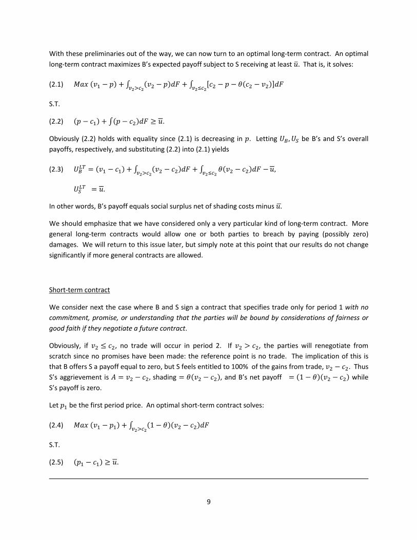
With these preliminaries out of the way, we can now turn to an optimal long-term contract. An optimal long-term contract maximizes B’s expected payoff subject to S receiving at least 𝑢𝑢� . That is, it solves:

(2.1) 𝑀𝑀𝑀𝑀𝑀𝑀 (𝑣𝑣1 − 𝑝𝑝) + ∫ (𝑣𝑣2 − 𝑝𝑝)𝑑𝑑𝐹𝐹 + ∫ [𝑐𝑐2 − 𝑝𝑝 − 𝜃𝜃(𝑐𝑐2 − 𝑣𝑣2)]𝑑𝑑𝐹𝐹𝑣𝑣2≤𝑐𝑐2𝑣𝑣2>𝑐𝑐2

S.T.

(2.2) (𝑝𝑝 − 𝑐𝑐1) + ∫(𝑝𝑝 − 𝑐𝑐2)𝑑𝑑𝐹𝐹 ≥ 𝑢𝑢.

Obviously (2.2) holds with equality since (2.1) is decreasing in 𝑝𝑝. Letting 𝑈𝑈𝐵𝐵,𝑈𝑈𝑆𝑆 be B’s and S’s overall payoffs, respectively, and substituting (2.2) into (2.1) yields

(2.3) 𝑈𝑈𝐵𝐵𝐿𝐿𝐿𝐿 = (𝑣𝑣1 − 𝑐𝑐1) + ∫ (𝑣𝑣2 − 𝑐𝑐2)𝑑𝑑𝐹𝐹 + ∫ 𝜃𝜃(𝑣𝑣2 − 𝑐𝑐2)𝑑𝑑𝐹𝐹 −𝑣𝑣2≤𝑐𝑐2𝑣𝑣2>𝑐𝑐2𝑢𝑢,

𝑈𝑈𝑆𝑆𝐿𝐿𝐿𝐿 = 𝑢𝑢.

In other words, B’s payoff equals social surplus net of shading costs minus 𝑢𝑢.�

We should emphasize that we have considered only a very particular kind of long-term contract. More general long-term contracts would allow one or both parties to breach by paying (possibly zero) damages. We will return to this issue later, but simply note at this point that our results do not change significantly if more general contracts are allowed.

Short-term contract

We consider next the case where B and S sign a contract that specifies trade only for period 1 with no commitment, promise, or understanding that the parties will be bound by considerations of fairness or good faith if they negotiate a future contract.

Obviously, if 𝑣𝑣2 ≤ 𝑐𝑐2, no trade will occur in period 2. If 𝑣𝑣2 > 𝑐𝑐2, the parties will renegotiate from scratch since no promises have been made: the reference point is no trade. The implication of this is that B offers S a payoff equal to zero, but S feels entitled to 100% of the gains from trade, 𝑣𝑣2 − 𝑐𝑐2. Thus S’s aggrievement is 𝜃𝜃 = 𝑣𝑣2 − 𝑐𝑐2, shading = 𝜃𝜃(𝑣𝑣2 − 𝑐𝑐2), and B’s net payoff = (1 − 𝜃𝜃)(𝑣𝑣2 − 𝑐𝑐2) while S’s payoff is zero.

Let 𝑝𝑝1 be the first period price. An optimal short-term contract solves:

(2.4) 𝑀𝑀𝑀𝑀𝑀𝑀 (𝑣𝑣1 − 𝑝𝑝1) + ∫ (1 − 𝜃𝜃)(𝑣𝑣2 − 𝑐𝑐2)𝑑𝑑𝐹𝐹𝑣𝑣2>𝑐𝑐2

S.T.

(2.5) (𝑝𝑝1 − 𝑐𝑐1) ≥ 𝑢𝑢.

9

Again (2.5) holds with equality since B can always gain from reducing 𝑝𝑝1. Hence

(2.6) 𝑈𝑈𝐵𝐵𝑆𝑆𝐿𝐿 = (𝑣𝑣1 − 𝑐𝑐1) + ∫ (1 − 𝜃𝜃)(𝑣𝑣2 − 𝑐𝑐2)𝑑𝑑𝐹𝐹 −𝑣𝑣2>𝑐𝑐2𝑢𝑢,

𝑈𝑈𝑆𝑆𝑆𝑆𝐿𝐿 = 𝑢𝑢.

As above, B’s payoff equals social surplus net of shading costs minus 𝑢𝑢.�

Continuing contract

We now turn to what we call a continuing contract. A continuing contract is a contract that specifies trade in the first period, does not commit the parties to trade in the second period, but includes some commitment, promise, or understanding that the parties will be bound by considerations of fairness or good faith if they do negotiate a future contract.

We formalize the idea of fairness or good faith as follows. At date 1, if 𝑣𝑣2 ≤ 𝑐𝑐2, the parties walk away and surplus is zero22. However, if 𝑣𝑣2 > 𝑐𝑐2, they bargain using the period 1 contract as a reference point. If conditions have not changed much, that is, 𝑣𝑣2 ≈ 𝑣𝑣1, 𝑐𝑐2 ≈ 𝑐𝑐1, then good faith means that the price should not change much. (There is an exception to this, noted below, if 𝑝𝑝1 < 𝑐𝑐1 or 𝑝𝑝1 > 𝑣𝑣1.) On the other hand, if 𝑣𝑣2 or 𝑐𝑐2 do change relative to 𝑣𝑣1, 𝑐𝑐1, then good faith means that the price can change but only commensurate with the changes in 𝑣𝑣 and 𝑐𝑐.

To be precise, suppose 𝑣𝑣2 > 𝑐𝑐2, and let ∆𝐺𝐺 = (𝑣𝑣2 − 𝑐𝑐2) − (𝑣𝑣1 − 𝑐𝑐1). We distinguish between the cases ∆𝐺𝐺 ≥ 0 and ∆𝐺𝐺 < 0. Previously we assumed that each party feels entitled to 100% of any change in surplus. However, that was for the case where the change was always positive. We now assume that B and S’s self-serving biases are such that each party feels entitled to any increase in surplus but feels that the other should suffer any decrease in surplus. However, both regard the initial contract as a reference point.

Before continuing, we should note that our assumption that the parties focus on changes in surplus rather than changes in 𝑣𝑣, 𝑐𝑐 independently is only one of several possibilities. It would also be plausible to assume that B attributes increases in 𝑣𝑣 (resp., 𝑐𝑐) to B’s (resp.,S’s) actions or talent and decreases in 𝑣𝑣 (resp., 𝑐𝑐) to luck; and vice versa for S. This would change some details but not the thrust of the analysis. The important thing is that it is changes in 𝑣𝑣, 𝑐𝑐 not absolute values that matter in a continuing contract.

It is also worth discussing a little further what we have in mind when we assume that changes in 𝑣𝑣, 𝑐𝑐 can be observed by both parties but are not verifiable and so cannot be part of an indexed contract. Imagine that 𝑐𝑐 rises. S knows this and can perhaps produce an argument or evidence to B that will

22 We are ruling out the possibility that one or other party might feel aggrieved and shade in the event that trade does not occur given that it could have; for example, if S’s cost is low she might be angry with B that his value is even lower. Note that it might be difficult for S to shade against B under these conditions since B walks away and no trade takes place. A similar assumption is made in Hart and Moore (2008): shading cannot occur if one party walks away.

10

persuade him that this is indeed the case. However, if the parties wrote an ex ante contract that said that price will rise if S produces evidence that c has risen, then this could lead to abuse: S could produce something that looks like evidence but isn’t really. In other words, the observability but nonverifiability of evidence can justify the assumption that changes in 𝑣𝑣, 𝑐𝑐 are observable but not verifiable.

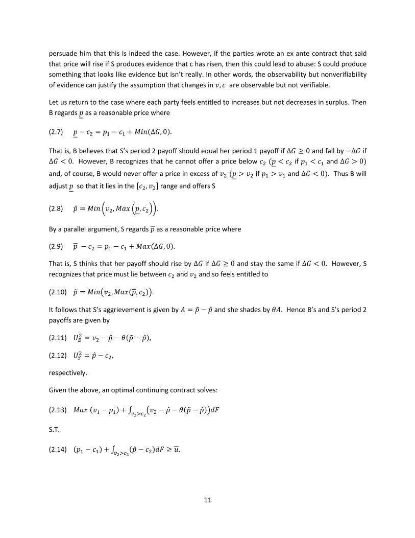
Let us return to the case where each party feels entitled to increases but not decreases in surplus. Then B regards 𝑝𝑝 as a reasonable price where

(2.7) 𝑝𝑝 − 𝑐𝑐2 = 𝑝𝑝1 − 𝑐𝑐1 + 𝑀𝑀𝑀𝑀𝑀𝑀(∆𝐺𝐺, 0).

That is, B believes that S’s period 2 payoff should equal her period 1 payoff if ∆𝐺𝐺 ≥ 0 and fall by −∆𝐺𝐺 if ∆𝐺𝐺 < 0. However, B recognizes that he cannot offer a price below 𝑐𝑐2 (𝑝𝑝 < 𝑐𝑐2 if 𝑝𝑝1 < 𝑐𝑐1 and ∆𝐺𝐺 > 0)

and, of course, B would never offer a price in excess of 𝑣𝑣2 (𝑝𝑝 > 𝑣𝑣2 if 𝑝𝑝1 > 𝑣𝑣1 and ∆𝐺𝐺 < 0). Thus B will

adjust 𝑝𝑝 so that it lies in the [𝑐𝑐2, 𝑣𝑣2] range and offers S

(2.8) �̂�𝑝 = 𝑀𝑀𝑀𝑀𝑀𝑀 �𝑣𝑣2,𝑀𝑀𝑀𝑀𝑀𝑀 �𝑝𝑝, 𝑐𝑐2��.

By a parallel argument, S regards 𝑝𝑝 as a reasonable price where

(2.9) 𝑝𝑝 − 𝑐𝑐2 = 𝑝𝑝1 − 𝑐𝑐1 +𝑀𝑀𝑀𝑀𝑀𝑀(∆𝐺𝐺, 0).

That is, S thinks that her payoff should rise by ∆𝐺𝐺 if ∆𝐺𝐺 ≥ 0 and stay the same if ∆𝐺𝐺 < 0. However, S recognizes that price must lie between 𝑐𝑐2 and 𝑣𝑣2 and so feels entitled to

(2.10) 𝑝𝑝� = 𝑀𝑀𝑀𝑀𝑀𝑀�𝑣𝑣2,𝑀𝑀𝑀𝑀𝑀𝑀(𝑝𝑝, 𝑐𝑐2)�.

It follows that S’s aggrievement is given by 𝜃𝜃 = 𝑝𝑝� − �̂�𝑝 and she shades by 𝜃𝜃𝜃𝜃. Hence B’s and S’s period 2 payoffs are given by

(2.11) 𝑈𝑈𝐵𝐵2 = 𝑣𝑣2 − �̂�𝑝 − 𝜃𝜃(𝑝𝑝� − �̂�𝑝),

(2.12) 𝑈𝑈𝑆𝑆2 = �̂�𝑝 − 𝑐𝑐2,

respectively.

Given the above, an optimal continuing contract solves:

(2.13) 𝑀𝑀𝑀𝑀𝑀𝑀 (𝑣𝑣1 − 𝑝𝑝1) + ∫ �𝑣𝑣2 − �̂�𝑝 − 𝜃𝜃(𝑝𝑝� − �̂�𝑝)�𝑑𝑑𝐹𝐹𝑣𝑣2>𝑐𝑐2

S.T.

(2.14) (𝑝𝑝1 − 𝑐𝑐1) + ∫ (�̂�𝑝 − 𝑐𝑐2)𝑑𝑑𝐹𝐹𝑣𝑣2>𝑐𝑐2≥ 𝑢𝑢.

11

It is easy to see that (2.14) holds with equality: if not, reducing 𝑝𝑝1 a little reduces �̂�𝑝 and 𝑝𝑝� and hence raises 𝑣𝑣2 − (1 − 𝜃𝜃)�̂�𝑝 − 𝜃𝜃𝑝𝑝�, which increases (2.13)23. Substituting (2.14) into (2.13) we can write the parties’ payoffs as

(2.15) 𝑈𝑈𝐵𝐵𝐶𝐶 = (𝑣𝑣1 − 𝑐𝑐1) + ∫ [𝑣𝑣2 − 𝑐𝑐2 − 𝜃𝜃(𝑝𝑝� − �̂�𝑝)]𝑑𝑑𝐹𝐹 −𝑣𝑣2>𝑐𝑐2𝑢𝑢,

𝑈𝑈𝑆𝑆𝐶𝐶 = 𝑢𝑢.

Note that 𝑝𝑝1 affects (𝑝𝑝� − �̂�𝑝) and so is still present in (2.15). Thus in contrast to a short-term or long-term contract it is not the case that 𝑈𝑈𝐵𝐵𝐶𝐶 changes one to one with 𝑢𝑢.

At this point an example may help. Suppose that 𝑣𝑣1 = 20, 𝑐𝑐1 = 10 and 𝑝𝑝1 = 15. Assume that at date 1 it is learned that 𝑣𝑣2 = 24, 𝑐𝑐2 = 10 (surplus goes up by 4). Then with a continuing contract B will regard 15 as the appropriate price (this gives all the additional surplus to B), while S will regard 19 as the appropriate price (this gives all the additional surplus to S). B will offer 15 but S will be aggrieved by 4 and will shade by 4𝜃𝜃.

Suppose instead that it is learned that 𝑣𝑣2 = 24, 𝑐𝑐2 = 20 (surplus goes down by 6). Now B regards 19 as the right price since this makes S bear the full decrease in surplus. However, S will not trade at 19 and so B adjusts his notion of entitlement so that 20 becomes a reasonable price. S regards 25 as a reasonable price by a similar argument, but since B will not trade at this price she adjusts her entitlement to 24. Thus B will offer 20 but S will be aggrieved by 4 and will shade by 4𝜃𝜃.

We now turn to a comparison of long-term, short-term, and continuing contracts. In the case of no outside options it is easy to show that a continuing contract is always at least as good for B as a short-term contract (S is indifferent since she always gets 𝑢𝑢).

Proposition 1. With no outside options, 𝑈𝑈𝐵𝐵𝐶𝐶 ≥ 𝑈𝑈𝐵𝐵𝑆𝑆𝐿𝐿.

Proof: Consider an optimal continuing contract. We know from (2.15) that

(2.16) 𝑈𝑈𝐵𝐵𝐶𝐶 = (𝑣𝑣1 − 𝑐𝑐1) + ∫ [𝑣𝑣2 − 𝑐𝑐2 − 𝜃𝜃(𝑝𝑝� − �̂�𝑝)]𝑑𝑑𝐹𝐹 −𝑣𝑣2>𝑐𝑐2𝑢𝑢

≥ (𝑣𝑣1 − 𝑐𝑐1) + ∫ (1 − 𝜃𝜃)(𝑣𝑣2 − 𝑐𝑐2)𝑑𝑑𝐹𝐹 −𝑣𝑣2>𝑐𝑐2𝑢𝑢 = 𝑈𝑈𝐵𝐵𝑆𝑆𝐿𝐿 ,

where the inequality follows from the fact that 𝑝𝑝� − �̂�𝑝 ≤ 𝑣𝑣2 − 𝑐𝑐2. Q.E.D.

In other words, in this very simple setting, good faith is always a plus: it reduces aggrievement and shading since, with the first period contract as a reference point, there is less to argue about in period 2.

23 Note that 𝑝𝑝1 plays two roles. It acts as a reference point for the period 2 price and it also serves to distribute surplus. We are ruling out the possibility that a lump sum transfer can be used to distribute surplus independently of the first period price. Our assumption is that, if this were attempted, the parties would “see through it” and use the average of the two as a reference point.

12

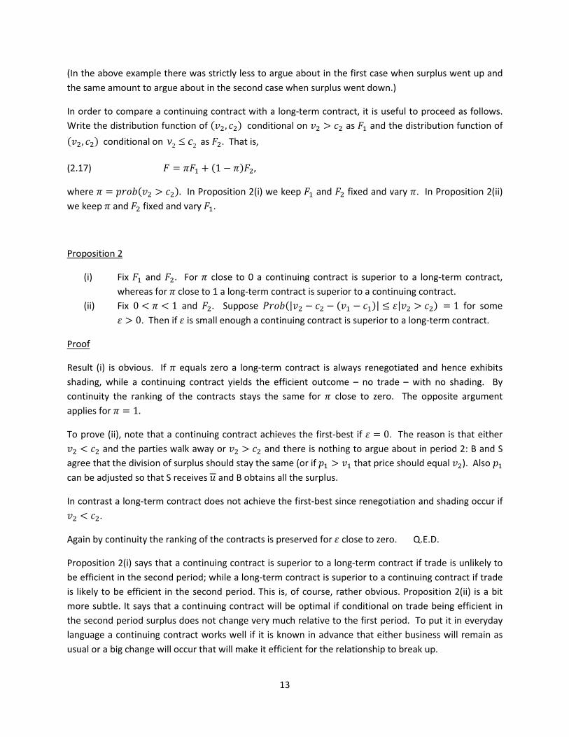
(In the above example there was strictly less to argue about in the first case when surplus went up and the same amount to argue about in the second case when surplus went down.)

In order to compare a continuing contract with a long-term contract, it is useful to proceed as follows. Write the distribution function of (𝑣𝑣2, 𝑐𝑐2) conditional on 𝑣𝑣2 > 𝑐𝑐2 as 𝐹𝐹1 and the distribution function of (𝑣𝑣2, 𝑐𝑐2) conditional on 2 2v c≤ as 𝐹𝐹2. That is,

(2.17) 𝐹𝐹 = 𝜋𝜋𝐹𝐹1 + (1 − 𝜋𝜋)𝐹𝐹2,

where 𝜋𝜋 = 𝑝𝑝𝑟𝑟𝑝𝑝𝑝𝑝(𝑣𝑣2 > 𝑐𝑐2). In Proposition 2(i) we keep 𝐹𝐹1 and 𝐹𝐹2 fixed and vary 𝜋𝜋. In Proposition 2(ii) we keep 𝜋𝜋 and 𝐹𝐹2 fixed and vary 𝐹𝐹1.

Proposition 2

(i) Fix 𝐹𝐹1 and 𝐹𝐹2. For 𝜋𝜋 close to 0 a continuing contract is superior to a long-term contract, whereas for 𝜋𝜋 close to 1 a long-term contract is superior to a continuing contract.

(ii) Fix 0 < 𝜋𝜋 < 1 and 𝐹𝐹2. Suppose 𝑃𝑃𝑟𝑟𝑝𝑝𝑝𝑝(|𝑣𝑣2 − 𝑐𝑐2 − (𝑣𝑣1 − 𝑐𝑐1)| ≤ 𝜀𝜀|𝑣𝑣2 > 𝑐𝑐2) = 1 for some 𝜀𝜀 > 0. Then if 𝜀𝜀 is small enough a continuing contract is superior to a long-term contract.

Proof

Result (i) is obvious. If 𝜋𝜋 equals zero a long-term contract is always renegotiated and hence exhibits shading, while a continuing contract yields the efficient outcome – no trade – with no shading. By continuity the ranking of the contracts stays the same for 𝜋𝜋 close to zero. The opposite argument applies for 𝜋𝜋 = 1.

To prove (ii), note that a continuing contract achieves the first-best if 𝜀𝜀 = 0. The reason is that either 𝑣𝑣2 < 𝑐𝑐2 and the parties walk away or 𝑣𝑣2 > 𝑐𝑐2 and there is nothing to argue about in period 2: B and S agree that the division of surplus should stay the same (or if 𝑝𝑝1 > 𝑣𝑣1 that price should equal 𝑣𝑣2). Also 𝑝𝑝1 can be adjusted so that S receives 𝑢𝑢 and B obtains all the surplus.

In contrast a long-term contract does not achieve the first-best since renegotiation and shading occur if 𝑣𝑣2 < 𝑐𝑐2.

Again by continuity the ranking of the contracts is preserved for 𝜀𝜀 close to zero. Q.E.D.

Proposition 2(i) says that a continuing contract is superior to a long-term contract if trade is unlikely to be efficient in the second period; while a long-term contract is superior to a continuing contract if trade is likely to be efficient in the second period. This is, of course, rather obvious. Proposition 2(ii) is a bit more subtle. It says that a continuing contract will be optimal if conditional on trade being efficient in the second period surplus does not change very much relative to the first period. To put it in everyday language a continuing contract works well if it is known in advance that either business will remain as usual or a big change will occur that will make it efficient for the relationship to break up.

13

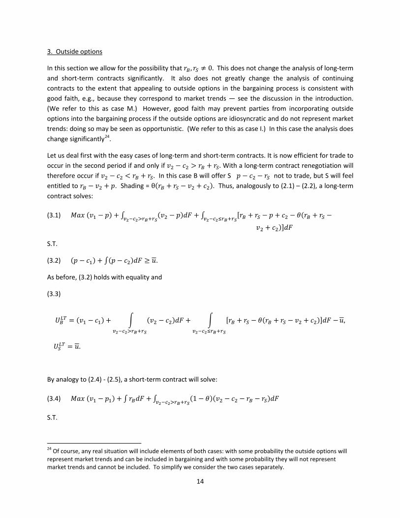
3. Outside options

In this section we allow for the possibility that 𝑟𝑟𝐵𝐵, 𝑟𝑟𝑆𝑆 ≠ 0. This does not change the analysis of long-term and short-term contracts significantly. It also does not greatly change the analysis of continuing contracts to the extent that appealing to outside options in the bargaining process is consistent with good faith, e.g., because they correspond to market trends — see the discussion in the introduction. (We refer to this as case M.) However, good faith may prevent parties from incorporating outside options into the bargaining process if the outside options are idiosyncratic and do not represent market trends: doing so may be seen as opportunistic. (We refer to this as case I.) In this case the analysis does change significantly24.

Let us deal first with the easy cases of long-term and short-term contracts. It is now efficient for trade to occur in the second period if and only if 𝑣𝑣2 − 𝑐𝑐2 > 𝑟𝑟𝐵𝐵 + 𝑟𝑟𝑆𝑆. With a long-term contract renegotiation will therefore occur if 𝑣𝑣2 − 𝑐𝑐2 < 𝑟𝑟𝐵𝐵 + 𝑟𝑟𝑆𝑆. In this case B will offer S 𝑝𝑝 − 𝑐𝑐2 − 𝑟𝑟𝑆𝑆 not to trade, but S will feel entitled to 𝑟𝑟𝐵𝐵 − 𝑣𝑣2 + 𝑝𝑝. Shading = θ(𝑟𝑟𝐵𝐵 + 𝑟𝑟𝑆𝑆 − 𝑣𝑣2 + 𝑐𝑐2). Thus, analogously to (2.1) – (2.2), a long-term contract solves:

(3.1) 𝑀𝑀𝑀𝑀𝑀𝑀 (𝑣𝑣1 − 𝑝𝑝) + ∫ (𝑣𝑣2 − 𝑝𝑝)𝑑𝑑𝐹𝐹 + ∫ [𝑟𝑟𝐵𝐵 + 𝑟𝑟𝑆𝑆 − 𝑝𝑝 + 𝑐𝑐2 − 𝜃𝜃(𝑟𝑟𝐵𝐵 + 𝑟𝑟𝑆𝑆 −𝑣𝑣2−𝑐𝑐2≤𝑟𝑟𝐵𝐵+𝑟𝑟𝑆𝑆𝑣𝑣2−𝑐𝑐2>𝑟𝑟𝐵𝐵+𝑟𝑟𝑆𝑆 𝑣𝑣2 + 𝑐𝑐2)]𝑑𝑑𝐹𝐹

S.T.

(3.2) (𝑝𝑝 − 𝑐𝑐1) + ∫(𝑝𝑝 − 𝑐𝑐2)𝑑𝑑𝐹𝐹 ≥ 𝑢𝑢.

As before, (3.2) holds with equality and

(3.3)

𝑈𝑈𝐵𝐵𝐿𝐿𝐿𝐿 = (𝑣𝑣1 − 𝑐𝑐1) + � (𝑣𝑣2 − 𝑐𝑐2)𝑑𝑑𝐹𝐹 + � [𝑟𝑟𝐵𝐵 + 𝑟𝑟𝑆𝑆 − 𝜃𝜃(𝑟𝑟𝐵𝐵 + 𝑟𝑟𝑆𝑆 − 𝑣𝑣2 + 𝑐𝑐2)]𝑑𝑑𝐹𝐹 −𝑣𝑣2−𝑐𝑐2≤𝑟𝑟𝐵𝐵+𝑟𝑟𝑆𝑆𝑣𝑣2−𝑐𝑐2>𝑟𝑟𝐵𝐵+𝑟𝑟𝑆𝑆

𝑢𝑢,

𝑈𝑈𝑆𝑆𝐿𝐿𝐿𝐿 = 𝑢𝑢.

By analogy to (2.4) - (2.5), a short-term contract will solve:

(3.4) 𝑀𝑀𝑀𝑀𝑀𝑀 (𝑣𝑣1 − 𝑝𝑝1) + ∫ 𝑟𝑟𝐵𝐵𝑑𝑑𝐹𝐹 + ∫ (1 − 𝜃𝜃)(𝑣𝑣2 − 𝑐𝑐2 − 𝑟𝑟𝐵𝐵 − 𝑟𝑟𝑆𝑆)𝑑𝑑𝐹𝐹𝑣𝑣2−𝑐𝑐2>𝑟𝑟𝐵𝐵+𝑟𝑟𝑆𝑆

S.T.

24 Of course, any real situation will include elements of both cases: with some probability the outside options will represent market trends and can be included in bargaining and with some probability they will not represent market trends and cannot be included. To simplify we consider the two cases separately.

14

(3.5) (𝑝𝑝1 − 𝑐𝑐1) + ∫ 𝑟𝑟𝑆𝑆𝑑𝑑𝐹𝐹 ≥ 𝑢𝑢.

(3.5) holds with equality and so

(3.6) 𝑈𝑈𝐵𝐵𝑆𝑆𝐿𝐿 = (𝑣𝑣1 − 𝑐𝑐1) + ∫(𝑟𝑟𝐵𝐵 + 𝑟𝑟𝑆𝑆)𝑑𝑑𝐹𝐹 + ∫ (1 − 𝜃𝜃)(𝑣𝑣2 − 𝑐𝑐2 − 𝑟𝑟𝐵𝐵 − 𝑟𝑟𝑆𝑆)𝑑𝑑𝐹𝐹 −𝑣𝑣2−𝑐𝑐2>𝑟𝑟𝐵𝐵+𝑟𝑟𝑆𝑆𝑢𝑢,

𝑈𝑈𝑆𝑆𝑆𝑆𝐿𝐿 = 𝑢𝑢.

Consider next a continuing contract. Start with case M where outside options can be used in the bargaining. Suppose 𝑣𝑣2 − 𝑐𝑐2 > 𝑟𝑟𝐵𝐵 + 𝑟𝑟𝑆𝑆 . Then the analysis is similar to that of Section 2. B thinks that 𝑝𝑝

is a reasonable price but recognizes that price must lie in the [𝑐𝑐2 + 𝑟𝑟𝑆𝑆, 𝑣𝑣2 − 𝑟𝑟𝐵𝐵] range and so offers S

(3.7) �̂�𝑝𝑀𝑀 = 𝑀𝑀𝑀𝑀𝑀𝑀 �𝑣𝑣2 − 𝑟𝑟𝐵𝐵,𝑀𝑀𝑀𝑀𝑀𝑀 �𝑝𝑝, 𝑐𝑐2 + 𝑟𝑟𝑆𝑆��.

S thinks that 𝑝𝑝 is a reasonable price but recognizes that price must lie in the [𝑐𝑐2 + 𝑟𝑟𝑆𝑆, 𝑣𝑣2 − 𝑟𝑟𝐵𝐵] range and so adjusts her entitlement to

(3.8) 𝑝𝑝�𝑀𝑀 = 𝑀𝑀𝑀𝑀𝑀𝑀�𝑣𝑣2 − 𝑟𝑟𝐵𝐵,𝑀𝑀𝑀𝑀𝑀𝑀(𝑝𝑝, 𝑐𝑐2 + 𝑟𝑟𝑆𝑆)� .

In other words in case M each party is willing to adjust the price to match the other party’s outside option if there are gains from trade. Note that (3.7) and (3.8) are not simply (2.8) and (2.10) with 𝑣𝑣2, 𝑐𝑐2 replaced by 𝑣𝑣2 − 𝑟𝑟𝐵𝐵 , 𝑐𝑐2 + 𝑟𝑟𝑆𝑆. The reason is that the formulae for 𝑝𝑝 , 𝑝𝑝 depend on 𝑣𝑣2, 𝑐𝑐2 not 𝑣𝑣2 − 𝑟𝑟𝐵𝐵 ,

𝑐𝑐2 + 𝑟𝑟𝑆𝑆.25

An optimal continuing contract solves:

(3.9) 𝑀𝑀𝑀𝑀𝑀𝑀 (𝑣𝑣1 − 𝑝𝑝1) + ∫ �𝑣𝑣2 − �̂�𝑝𝑀𝑀 − 𝜃𝜃(𝑝𝑝�𝑀𝑀 − �̂�𝑝𝑀𝑀)�𝑑𝑑𝐹𝐹𝑣𝑣2−𝑐𝑐2>𝑟𝑟𝐵𝐵+𝑟𝑟𝑆𝑆+ ∫ 𝑟𝑟𝐵𝐵𝑑𝑑𝐹𝐹𝑣𝑣2−𝑐𝑐2≤𝑟𝑟𝐵𝐵+𝑟𝑟𝑆𝑆

S.T.

(3.10) (𝑝𝑝1 − 𝑐𝑐1) + ∫ (�̂�𝑝𝑀𝑀 − 𝑐𝑐2)𝑑𝑑𝐹𝐹𝑣𝑣2−𝑐𝑐2>𝑟𝑟𝐵𝐵+𝑟𝑟𝑆𝑆+ ∫ 𝑟𝑟𝑆𝑆𝑑𝑑𝐹𝐹𝑣𝑣2−𝑐𝑐2≤𝑟𝑟𝐵𝐵+𝑟𝑟𝑆𝑆

≥ 𝑢𝑢.

As before, (3.10) holds with equality and so we obtain

25 For example, suppose 𝑣𝑣1 = 20, 𝑐𝑐1 = 10 and 𝑝𝑝1 = 15. At date 1 it is learned that 𝑣𝑣2 = 24, 𝑐𝑐2 = 10, 𝑟𝑟𝐵𝐵 =0, 𝑟𝑟𝑆𝑆 = 11. Then �̂�𝑝𝑀𝑀 = 𝑝𝑝�𝑀𝑀 = 21 and there is nothing to argue about. In contrast, if we replace 𝑐𝑐2 by 𝑐𝑐2 + 𝑟𝑟𝑆𝑆 =11 and set 𝑟𝑟𝑆𝑆 = 0 then according to the logic of Section 2 �̂�𝑝 =24, 𝑝𝑝� = 21 and there is something to argue about.

15

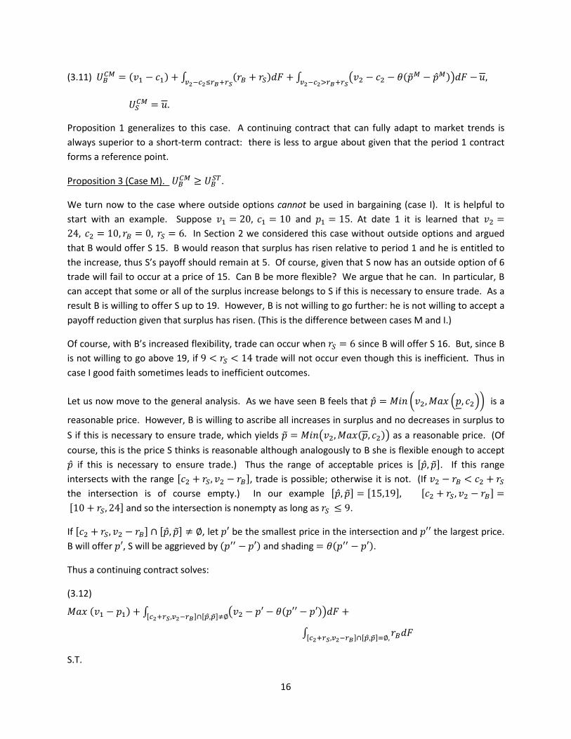
(3.11) 𝑈𝑈𝐵𝐵𝐶𝐶𝑀𝑀 = (𝑣𝑣1 − 𝑐𝑐1) + ∫ (𝑟𝑟𝐵𝐵 + 𝑟𝑟𝑆𝑆)𝑑𝑑𝐹𝐹𝑣𝑣2−𝑐𝑐2≤𝑟𝑟𝐵𝐵+𝑟𝑟𝑆𝑆+ ∫ �𝑣𝑣2 − 𝑐𝑐2 − 𝜃𝜃(𝑝𝑝�𝑀𝑀 − �̂�𝑝𝑀𝑀)�𝑑𝑑𝐹𝐹 −𝑣𝑣2−𝑐𝑐2>𝑟𝑟𝐵𝐵+𝑟𝑟𝑆𝑆

𝑢𝑢,

𝑈𝑈𝑆𝑆𝐶𝐶𝑀𝑀 = 𝑢𝑢.

Proposition 1 generalizes to this case. A continuing contract that can fully adapt to market trends is always superior to a short-term contract: there is less to argue about given that the period 1 contract forms a reference point.

Proposition 3 (Case M). 𝑈𝑈𝐵𝐵𝐶𝐶𝑀𝑀 ≥ 𝑈𝑈𝐵𝐵𝑆𝑆𝐿𝐿.

We turn now to the case where outside options cannot be used in bargaining (case I). It is helpful to start with an example. Suppose 𝑣𝑣1 = 20, 𝑐𝑐1 = 10 and 𝑝𝑝1 = 15. At date 1 it is learned that 𝑣𝑣2 =24, 𝑐𝑐2 = 10, 𝑟𝑟𝐵𝐵 = 0, 𝑟𝑟𝑆𝑆 = 6. In Section 2 we considered this case without outside options and argued that B would offer S 15. B would reason that surplus has risen relative to period 1 and he is entitled to the increase, thus S’s payoff should remain at 5. Of course, given that S now has an outside option of 6 trade will fail to occur at a price of 15. Can B be more flexible? We argue that he can. In particular, B can accept that some or all of the surplus increase belongs to S if this is necessary to ensure trade. As a result B is willing to offer S up to 19. However, B is not willing to go further: he is not willing to accept a payoff reduction given that surplus has risen. (This is the difference between cases M and I.)

Of course, with B’s increased flexibility, trade can occur when 𝑟𝑟𝑆𝑆 = 6 since B will offer S 16. But, since B is not willing to go above 19, if 9 < 𝑟𝑟𝑆𝑆 < 14 trade will not occur even though this is inefficient. Thus in case I good faith sometimes leads to inefficient outcomes.

Let us now move to the general analysis. As we have seen B feels that �̂�𝑝 = 𝑀𝑀𝑀𝑀𝑀𝑀 �𝑣𝑣2,𝑀𝑀𝑀𝑀𝑀𝑀 �𝑝𝑝, 𝑐𝑐2�� is a

reasonable price. However, B is willing to ascribe all increases in surplus and no decreases in surplus to S if this is necessary to ensure trade, which yields 𝑝𝑝� = 𝑀𝑀𝑀𝑀𝑀𝑀�𝑣𝑣2,𝑀𝑀𝑀𝑀𝑀𝑀(𝑝𝑝, 𝑐𝑐2)� as a reasonable price. (Of course, this is the price S thinks is reasonable although analogously to B she is flexible enough to accept �̂�𝑝 if this is necessary to ensure trade.) Thus the range of acceptable prices is [�̂�𝑝,𝑝𝑝�]. If this range intersects with the range [𝑐𝑐2 + 𝑟𝑟𝑆𝑆, 𝑣𝑣2 − 𝑟𝑟𝐵𝐵], trade is possible; otherwise it is not. (If 𝑣𝑣2 − 𝑟𝑟𝐵𝐵 < 𝑐𝑐2 + 𝑟𝑟𝑆𝑆 the intersection is of course empty.) In our example [�̂�𝑝,𝑝𝑝�] = [15,19], [𝑐𝑐2 + 𝑟𝑟𝑆𝑆, 𝑣𝑣2 − 𝑟𝑟𝐵𝐵] = [10 + 𝑟𝑟𝑆𝑆, 24] and so the intersection is nonempty as long as 𝑟𝑟𝑆𝑆 ≤ 9.

If [𝑐𝑐2 + 𝑟𝑟𝑆𝑆, 𝑣𝑣2 − 𝑟𝑟𝐵𝐵] ∩ [�̂�𝑝,𝑝𝑝�] ≠ ∅, let 𝑝𝑝′ be the smallest price in the intersection and 𝑝𝑝′′ the largest price. B will offer 𝑝𝑝′, S will be aggrieved by (𝑝𝑝′′ − 𝑝𝑝′) and shading = 𝜃𝜃(𝑝𝑝′′ − 𝑝𝑝′).

Thus a continuing contract solves:

(3.12)

𝑀𝑀𝑀𝑀𝑀𝑀 (𝑣𝑣1 − 𝑝𝑝1) + ∫ �𝑣𝑣2 − 𝑝𝑝′ − 𝜃𝜃(𝑝𝑝′′ − 𝑝𝑝′)�𝑑𝑑𝐹𝐹[𝑐𝑐2+𝑟𝑟𝑆𝑆 ,𝑣𝑣2−𝑟𝑟𝐵𝐵]∩[𝑝𝑝�,𝑝𝑝�]≠∅ +

∫ 𝑟𝑟𝐵𝐵𝑑𝑑𝐹𝐹[𝑐𝑐2+𝑟𝑟𝑆𝑆,𝑣𝑣2−𝑟𝑟𝐵𝐵]∩[𝑝𝑝�,𝑝𝑝�]=∅,

S.T.

16

(3.13) (𝑝𝑝1 − 𝑐𝑐1) + ∫ (𝑝𝑝′ − 𝑐𝑐2)𝑑𝑑𝐹𝐹[𝑐𝑐2+𝑟𝑟𝑆𝑆,𝑣𝑣2−𝑟𝑟𝐵𝐵]∩[𝑝𝑝�,𝑝𝑝�]≠∅ + ∫ 𝑟𝑟𝑆𝑆𝑑𝑑𝐹𝐹[𝑐𝑐2+𝑟𝑟𝑆𝑆 ,𝑣𝑣2−𝑟𝑟𝐵𝐵]∩[𝑝𝑝�,𝑝𝑝�]=∅ ≥ 𝑢𝑢.

An important difference from the M case is that (3.13) may not be binding at the optimum. The reason is that (3.12) may not be monotonic in 𝑝𝑝1 given that a lower 𝑝𝑝1 may lead to inefficient outcomes. In other words an “efficiency” wage (or price) may be optimal. Also it is no longer true that a continuing contract is always superior to a short-term contract. Example 3.1 illustrates both of these possibilities.

Example 3.1

There is no uncertainty, 𝑣𝑣1 = 20, 𝑐𝑐1 = 10,𝑣𝑣2 = 20, 𝑐𝑐2 = 10, 𝑟𝑟𝑆𝑆 = 1,𝑢𝑢 = 1.

Consider a continuing contract (case I). Suppose 10 ≤ 𝑝𝑝1 ≤ 20. Since 𝑣𝑣2 = 𝑣𝑣1, 𝑐𝑐2 = 𝑐𝑐1, 𝑝𝑝 = 𝑝𝑝 = 𝑝𝑝1

and so �̂�𝑝 = 𝑝𝑝� = 𝑝𝑝1. That is, 𝑝𝑝2 = 𝑝𝑝1: no change in price is possible. Hence, given S’s outside option in period 2, trade will occur in period 2 only if 𝑝𝑝2 = 𝑝𝑝1 ≥ 11. Given 𝑝𝑝1 ≥ 11, it is optimal for B to set 𝑝𝑝1 = 11: this ensures trade in both periods and yields 𝑈𝑈𝐵𝐵 = 18,𝑈𝑈𝑆𝑆 = 2. Alternatively, if 𝑝𝑝1 < 11, since no trade occurs in period 2, it is best for B to set 𝑝𝑝1 = 10. This yields 𝑈𝑈𝐵𝐵 = 10,𝑈𝑈𝑆𝑆 = 1. (It is easy to show that 𝑝𝑝1 < 10 or 𝑝𝑝1 > 20 is not optimal.)

Obviously the first contract is superior, and this gives S more than her reservation utility 𝑢𝑢. As promised (3.13) is not binding.

Now let’s compare the optimal continuing contract with a short-term contract. Under a short-term contract

𝑈𝑈𝑆𝑆𝑆𝑆𝐿𝐿 = 𝑝𝑝1 − 𝑐𝑐1 + 𝑟𝑟𝑆𝑆 = 𝑢𝑢

and so 𝑝𝑝1 = 10. Hence

𝑈𝑈𝐵𝐵𝑆𝑆𝐿𝐿 = 10 + (1 − 𝜃𝜃)9 = 19 − 9𝜃𝜃

> 18 = 𝑈𝑈𝐵𝐵𝐶𝐶𝐶𝐶

if 𝜃𝜃 < 19.

In other words, if 𝜃𝜃 < 19, a short-term contract is superior to a continuing contract: the reason is that the

shading cost is less than the benefit of keeping S at her reservation utility.

Of course, in this example, with no uncertainty, a long-term contract achieves the first-best since trade is always efficient. The next example shows that a short-term contract can be uniquely optimal for the idiosyncratic case.

17

Example 3.2 (Case I)

𝑣𝑣1 = 20, 𝑐𝑐1 = 10. There are three states of the world in period 2. In s1 (prob 𝜌𝜌/2) 𝑣𝑣2 = 20, 𝑐𝑐2 =10, 𝑟𝑟𝑆𝑆 = 3; in s2 (prob 𝜌𝜌/2) 𝑣𝑣2 = 20, 𝑐𝑐2 = 10, 𝑟𝑟𝑆𝑆 = 13; and in s3 (prob 1 − 𝜌𝜌) 𝑣𝑣2 = 10, 𝑐𝑐2 = 20, 𝑟𝑟𝑆𝑆 = 0. 𝑟𝑟𝐵𝐵 = 0 in all states.

Trade is efficient only in s1 in period 2.

Continuing contract

Under a continuing contract, trade never occurs in s2 or s3: the parties walk away. If 𝑝𝑝1 < 13, trade does not occur in s1 either since 𝑣𝑣 and 𝑐𝑐 have not changed and outside options cannot be used in bargaining: 𝑝𝑝2 = 𝑝𝑝1 and S will quit. Hence

𝑈𝑈𝑆𝑆𝐶𝐶𝐶𝐶 = 𝑝𝑝1 − 10 + 8𝜌𝜌,

𝑈𝑈𝐵𝐵𝐶𝐶𝐶𝐶 = 20 − 𝑝𝑝1,

which implies

𝑈𝑈𝐵𝐵𝐶𝐶𝐶𝐶 = 10 + 8𝜌𝜌 − 𝑈𝑈𝑆𝑆𝐶𝐶𝐶𝐶.

If 13 ≤ 𝑝𝑝1 ≤ 20, trade occurs in s1. Hence

𝑈𝑈𝑆𝑆𝐶𝐶𝐶𝐶 = 𝑝𝑝1 − 10 + (𝑝𝑝1 − 10)𝜌𝜌2

+13𝜌𝜌

2

= 𝑝𝑝1 �1 + 𝜌𝜌2� − 10 + 3𝜌𝜌

2 ,

𝑈𝑈𝐵𝐵𝐶𝐶𝐶𝐶 = (20 − 𝑝𝑝1) �1 +𝜌𝜌2�,

which implies

𝑈𝑈𝐵𝐵𝐶𝐶𝐶𝐶 = 10 + 23𝜌𝜌2− 𝑈𝑈𝑆𝑆𝐶𝐶𝐶𝐶.

18

The relationship between 𝑈𝑈𝐵𝐵𝐶𝐶𝐶𝐶 and 𝑈𝑈𝑆𝑆𝐶𝐶𝐶𝐶 is illustrated in Figure 2. Note that the discontinuity arises from

the fact that B would never choose 13 − 7𝜌𝜌2

< 𝑝𝑝1 < 13 as increasing 𝑝𝑝1 to 13 would result in trade in s1

and a higher expected payoff for B.

From Figure 2 it follows that an optimal continuing contract satisfies:

𝑈𝑈𝐵𝐵𝐶𝐶𝐶𝐶 = 10 + 8𝜌𝜌 − 𝑢𝑢� , 𝑈𝑈𝑆𝑆𝐶𝐶𝐶𝐶 = 𝑢𝑢� if 0 < 𝑢𝑢� < 3 + 9𝜌𝜌2

,

𝑈𝑈𝐵𝐵𝐶𝐶𝐶𝐶 = 7 + 7𝜌𝜌2

, 𝑈𝑈𝑆𝑆𝐶𝐶𝐶𝐶 = 3 + 8𝜌𝜌 if 3 + 9𝜌𝜌2≤ 𝑢𝑢� ≤ 3 + 8𝜌𝜌,

𝑈𝑈𝐵𝐵𝐶𝐶𝐶𝐶 = 10 + 23𝜌𝜌2− 𝑢𝑢� , 𝑈𝑈𝑆𝑆𝐶𝐶𝐶𝐶 = 𝑢𝑢� if 3 + 8𝜌𝜌 < 𝑢𝑢� ≤ 10 + 23𝜌𝜌

2.

For low values of 𝑢𝑢� pushing S down to her reservation utility implies such a low 𝑝𝑝1 that there will be an inefficient quit in s1. For intermediate values of 𝑢𝑢� B is better off raising 𝑝𝑝1 to 13 so that trade will take place in s1; this results in S getting more than her reservation utility. Finally, to satisfy S’s participation constraint for high values of 𝑢𝑢� 𝑝𝑝1 must be high enough so that trade will take place in s1. In this region a continuing contract achieves the first-best.

Long-term contract

A long-term contract requires renegotiation in s2 and s3. It is easily seen that

𝑈𝑈𝐵𝐵𝐿𝐿𝐿𝐿 = 10 +23𝜌𝜌

2+

17𝜌𝜌𝜃𝜃2

− 10𝜃𝜃 − 𝑢𝑢,�

19

𝑈𝑈𝑆𝑆𝐿𝐿𝐿𝐿 = 𝑢𝑢�.

Short-term contract

A short-term contract requires renegotiation in s1. It is easily seen that

𝑈𝑈𝐵𝐵𝑆𝑆𝐿𝐿 = 10 +23𝜌𝜌

2−

7𝜌𝜌𝜃𝜃2

− 𝑢𝑢,�

𝑈𝑈𝑆𝑆𝑆𝑆𝐿𝐿 = 𝑢𝑢�

It follows from the above that the (unique) optimal contract is:

(i) Short-term if and only if 𝜌𝜌 < 5/6 and 𝑢𝑢� < 3 + 8𝜌𝜌 − 72𝜌𝜌𝜃𝜃

(ii) Long-term if and only if 𝜌𝜌 > 5/6 and 𝑢𝑢� < 3 + 8𝜌𝜌 − �10 − 172𝜌𝜌� 𝜃𝜃

(iii) Continuing if and only if 𝑚𝑚𝑀𝑀𝑀𝑀 �3 + 8𝜌𝜌 − �10 − 172𝜌𝜌� 𝜃𝜃, 3 + 8𝜌𝜌 − 7

2𝜌𝜌𝜃𝜃� ≤ 𝑢𝑢� ≤ 10 + 23

2𝜌𝜌

We know that for low values of 𝑢𝑢� a continuing contract results in an inefficient quit. This is more costly for B than shading under either a short-term or a long-term contract. For high values of 𝑢𝑢� a continuing contract achieves the first-best. For intermediate values of 𝑢𝑢� there is a tradeoff. S receives more than her reservation utility under a continuing contract while a short-term or a long-term contract results in shading. Therefore, for the lower values of 𝑢𝑢� (in the intermediate range) the benefit of getting S down to her reservation utility outweighs the expected shading costs of a short-term or a long-term contract.

Based on Example 3.2, we can state the following proposition.

Proposition 4

In case I, the optimal contract can depend on 𝑢𝑢.

The intuition here is that while the comparison between a long-term contract and a short-term contract is independent of 𝑢𝑢 (in both cases 𝑢𝑢 is subtracted off the buyer’s payoff), the value of a continuing contract can depend on 𝑢𝑢 in a more complicated way since for some levels of 𝑢𝑢 the buyer will offer the seller an efficiency wage. As a result a continuing contract may be suboptimal for one level of 𝑢𝑢 but then as 𝑢𝑢 rises the buyer’s payoff under a continuing contract stays the same while it falls under a long-term or short-term contract. Hence a continuing contract can become favored for high values of 𝑢𝑢 . This is what happens in Example 3.2 above, where only the seller has an outside option. On the other hand, if the buyer has an outside option, an increase in 𝑢𝑢 can make a continuing contract less desirable since as 𝑝𝑝1 rises, the buyer will quit more often.

20

The next two propositions provide some general conditions under which the contracts can be ranked. They parallel Proposition 2 and as there it is useful to write

(3.18) 𝐹𝐹 = 𝜋𝜋𝐹𝐹1 + (1 − 𝜋𝜋)𝐹𝐹2,

where 𝐹𝐹1 is the distribution of (𝑣𝑣2, 𝑐𝑐2, 𝑟𝑟𝐵𝐵, 𝑟𝑟𝑆𝑆) conditional on 𝑣𝑣2 − 𝑐𝑐2 > 𝑟𝑟𝐵𝐵 + 𝑟𝑟𝑆𝑆, 𝐹𝐹2 is the distribution of (𝑣𝑣2, 𝑐𝑐2, 𝑟𝑟𝐵𝐵, 𝑟𝑟𝑆𝑆) conditional on 𝑣𝑣2 − 𝑐𝑐2 ≤ 𝑟𝑟𝐵𝐵 + 𝑟𝑟𝑆𝑆, and 𝜋𝜋 = 𝑃𝑃𝑟𝑟𝑝𝑝𝑝𝑝(𝑣𝑣2 − 𝑐𝑐2 > 𝑟𝑟𝐵𝐵 + 𝑟𝑟𝑆𝑆).

Proposition 5 (for case M)

(i) Fix 𝐹𝐹1 and 𝐹𝐹2. For 𝜋𝜋 close to zero, a short-term or continuing contract is superior to a long-term contract, whereas for 𝜋𝜋 close to 1 the reverse is the case.

(ii) Fix 0 < 𝜋𝜋 < 1. Suppose 𝑃𝑃𝑟𝑟𝑝𝑝𝑝𝑝(|𝑣𝑣2 − 𝑐𝑐2 − (𝑣𝑣1 − 𝑐𝑐1)| ≤ 𝜀𝜀|𝑣𝑣2 − 𝑐𝑐2 > 𝑟𝑟𝐵𝐵 + 𝑟𝑟𝑆𝑆) = 1 for some 𝜀𝜀 > 0. Then for 𝜀𝜀 small enough a continuing contract is optimal.

Proof

Part (i) is proved in the same way as in Proposition 2. To prove (ii), note that a continuing contract achieves the first-best if 𝜀𝜀 = 0. The reason is that either 𝑣𝑣2 − 𝑐𝑐2 ≤ 𝑟𝑟𝐵𝐵 + 𝑟𝑟𝑆𝑆 and the parties walk away or 𝑣𝑣2 − 𝑐𝑐2 > 𝑟𝑟𝐵𝐵 + 𝑟𝑟𝑆𝑆 and there is nothing to argue about in period 2: B and S agree that the division of surplus should stay the same subject to individual rationality and outside option constraints being satisfied. Also 𝑝𝑝1 can be adjusted so that S receives 𝑢𝑢 and B obtains all the surplus. Thus the first-best is achieved. Since a short-term or long-term contract does not achieve the first-best a continuing contract is optimal. By continuity the same is true if 𝜀𝜀 > 0 is small. Q.E.D.

Proposition 6 (for case I)

(i) Fix 𝐹𝐹1 and 𝐹𝐹2. For 𝜋𝜋 close to zero, a short-term or continuing contract is superior to a long-term contract, whereas for 𝜋𝜋 close to 1 the reverse is the case.

(ii) Fix 0 < 𝜋𝜋 < 1. Suppose 𝑃𝑃𝑟𝑟𝑝𝑝𝑝𝑝(|𝑣𝑣2 − 𝑐𝑐2 − (𝑣𝑣1 − 𝑐𝑐1)| ≤ 𝜀𝜀, 𝑟𝑟𝐵𝐵 ≤ 𝜀𝜀, 𝑟𝑟𝑆𝑆 ≤ 𝜀𝜀|𝑣𝑣2 − 𝑐𝑐2 > 𝑟𝑟𝐵𝐵 + 𝑟𝑟𝑆𝑆) = 1 for some 𝜀𝜀 > 0. Assume also 𝑢𝑢� ≥ 𝐸𝐸𝑟𝑟𝑆𝑆. Then for 𝜀𝜀 small enough a continuing contract is optimal.

(iii) Suppose there exist 𝑟𝑟1, 𝑟𝑟2 such that (𝑣𝑣1, 𝑐𝑐1, 𝑟𝑟1, 𝑟𝑟𝑆𝑆) ∈ support 𝐹𝐹1 for some 𝑟𝑟𝑆𝑆 and (𝑣𝑣1, 𝑐𝑐1, 𝑟𝑟𝐵𝐵, 𝑟𝑟2) ∈ support 𝐹𝐹1 for some 𝑟𝑟𝐵𝐵, where 𝑟𝑟1 + 𝑟𝑟2 > 𝑣𝑣1 − 𝑐𝑐1. Then for 𝜃𝜃 small enough a long-term or short-term contract is superior to a continuing contract.

Proof

Part (i) is proved in the same way as in Proposition 2. To prove (ii), note that a continuing contract achieves the first-best if 𝜀𝜀 = 0. The reason is that either 𝑣𝑣2 − 𝑐𝑐2 ≤ 𝑟𝑟𝐵𝐵 + 𝑟𝑟𝑆𝑆 and the parties walk away or 𝑣𝑣2 − 𝑐𝑐2 > 𝑟𝑟𝐵𝐵 + 𝑟𝑟𝑆𝑆 and there is nothing to argue about in period 2, and since 𝑟𝑟𝐵𝐵 = 𝑟𝑟𝑆𝑆 = 0 trade occurs. Also 𝑝𝑝1 can be adjusted so that S receives 𝑢𝑢 and B obtains all the surplus. Thus the

21

first-best is achieved. Finally, 𝑝𝑝1 ≥ 𝑐𝑐1 since 𝑢𝑢� ≥ 𝐸𝐸𝑟𝑟𝑆𝑆. Since a short-term or long-term contract does not achieve the first-best a continuing contract is optimal. By continuity the same is true if 𝜀𝜀 > 0 is small given that 𝑝𝑝1 can be adjusted slightly to ensure that trade continues to take place in the presence of small outside options.

To prove (iii), note that if 𝜃𝜃 is small a long-term or short-term contract approximates the first-best. In contrast a continuing contract does not since good faith bargaining leads to a second period price equal to 𝑝𝑝1 if 𝑣𝑣2 = 𝑣𝑣1, 𝑐𝑐2 = 𝑐𝑐1, and hence trade cannot occur in both (𝑣𝑣1, 𝑐𝑐1, 𝑟𝑟1, 𝑟𝑟𝑆𝑆) and (𝑣𝑣1, 𝑐𝑐1, 𝑟𝑟𝐵𝐵, 𝑟𝑟2): there will be inefficiency in a continuing contract. Q.E.D.

Proposition 5(ii) and 6(ii), like Proposition 4(ii), can be interpreted as saying that a continuing contract works well if it is known in advance that either business will remain as usual or a big change will occur that will make it efficient for the relationship to break up.

4. Renewable and Exclusive Contracts

We have studied a particular class of contracts. But there are other possibilities. We consider two in this section: renewable and exclusive contracts26.

4.1 Renewable Contracts

A renewable contract is a contract that specifies a first period price and a second period price, but allows either party to walk away in the second period. Another way to think of a renewable contract is that, concerning the second period, it is an “agreement to agree”. As mentioned in the introduction such contracts are observed in practice.

A renewable contract can then be represented by a first period price 𝑝𝑝1 and a second period price 𝑝𝑝2.27

Trade occurs in the second period if

(4.1) 𝑣𝑣2 − 𝑝𝑝2 ≥ 𝑟𝑟𝐵𝐵,

(4.2) 𝑝𝑝2 − 𝑐𝑐2 ≥ 𝑟𝑟𝑆𝑆.

26 We could consider other types of contracts, e.g., long-term contracts that that allow one of both parties to exit (or “breach”) but only if they pay damages; or contracts that give one or both parties an option to exercise trade in the second period. Doing so would not vitiate the relevance of the trade-offs discussed here. Note also that a renewable contract, discussed next, can be thought of as a long-term contract where either party can breach by paying zero damages. 27 We could consider a price range, with B choosing from this range ex post, instead of a single second period price (as in Hart and Moore (2008)). This would not change the analysis significantly.

22

If one of (4.1) - (4.2) fails to hold, but 𝑣𝑣2 − 𝑐𝑐2 > 𝑟𝑟𝐵𝐵 + 𝑟𝑟𝑆𝑆 the parties renegotiate. In this case B offers S a price 𝑝𝑝 = 𝑐𝑐2 + 𝑟𝑟𝑆𝑆, S feels entitled to 𝑣𝑣2 − 𝑟𝑟𝐵𝐵, and S shades by 𝜃𝜃(𝑣𝑣2 − 𝑐𝑐2 − 𝑟𝑟𝐵𝐵 − 𝑟𝑟𝑆𝑆). An optimal renewable contract solves:

(4.3) 𝑀𝑀𝑀𝑀𝑀𝑀 𝑣𝑣1 − 𝑝𝑝1 + ∫ (𝑣𝑣2 − 𝑝𝑝2)𝑣𝑣2−𝑝𝑝2≥𝑟𝑟𝐵𝐵,𝑝𝑝2−𝑐𝑐2≥𝑟𝑟𝑆𝑆 𝑑𝑑𝐹𝐹

+� [𝑣𝑣2 − 𝑐𝑐2 − 𝑟𝑟𝑆𝑆 − 𝜃𝜃(𝑣𝑣2 − 𝑐𝑐2 − 𝑟𝑟𝐵𝐵 − 𝑟𝑟𝑆𝑆)]𝑑𝑑𝐹𝐹 + � 𝑟𝑟𝐵𝐵𝑑𝑑𝐹𝐹𝑣𝑣2−𝑐𝑐2<𝑟𝑟𝐵𝐵+𝑟𝑟𝑆𝑆𝑣𝑣2−𝑐𝑐2>𝑟𝑟𝐵𝐵+𝑟𝑟𝑆𝑆 ,𝑣𝑣2−𝑝𝑝2<𝑟𝑟𝐵𝐵 𝑜𝑜𝑟𝑟 𝑝𝑝2−𝑐𝑐2<𝑟𝑟𝑆𝑆

S.T.

(4.4) 𝑝𝑝1 − 𝑐𝑐1 + ∫ (𝑝𝑝2 − 𝑐𝑐2)𝑑𝑑𝐹𝐹 +𝑣𝑣2−𝑝𝑝2≥𝑟𝑟𝐵𝐵,𝑝𝑝2−𝑐𝑐2≥𝑟𝑟𝑆𝑆∫ 𝑟𝑟𝑆𝑆𝑑𝑑𝐹𝐹 +𝑣𝑣2−𝑐𝑐2>𝑟𝑟𝐵𝐵+𝑟𝑟𝑆𝑆,𝑣𝑣2−𝑝𝑝2<𝑟𝑟𝐵𝐵 𝑜𝑜𝑟𝑟 𝑝𝑝2−𝑐𝑐2<𝑟𝑟𝑆𝑆

∫ 𝑟𝑟𝑆𝑆𝑑𝑑𝐹𝐹 ≥ 𝑢𝑢𝑣𝑣2−𝑐𝑐2<𝑟𝑟𝐵𝐵+𝑟𝑟𝑆𝑆.

Since (4.3) is decreasing in 𝑝𝑝1, (4.4) will be binding at the optimum. Thus we can write

(4.5) 𝑈𝑈𝐵𝐵𝑅𝑅 = 𝑀𝑀𝑀𝑀𝑀𝑀𝑝𝑝2 �𝑣𝑣1 − 𝑐𝑐1 + ∫(𝑟𝑟𝐵𝐵 + 𝑟𝑟𝑆𝑆)𝑑𝑑𝐹𝐹 + ∫ (𝑣𝑣2 − 𝑐𝑐2 − 𝑟𝑟𝐵𝐵 − 𝑟𝑟𝑆𝑆)𝑣𝑣2−𝑝𝑝2≥𝑟𝑟𝐵𝐵,𝑝𝑝2−𝑐𝑐2≥𝑟𝑟𝑆𝑆 𝑑𝑑𝐹𝐹 +

∫ [(1 − 𝜃𝜃)(𝑣𝑣2 − 𝑐𝑐2 − 𝑟𝑟𝐵𝐵 − 𝑟𝑟𝑆𝑆)]𝑑𝑑𝐹𝐹 − 𝑢𝑢𝑣𝑣2−𝑐𝑐2>𝑟𝑟𝐵𝐵+𝑟𝑟𝑆𝑆,𝑣𝑣2−𝑝𝑝2<𝑟𝑟𝐵𝐵 𝑜𝑜𝑟𝑟 𝑝𝑝2−𝑐𝑐2<𝑟𝑟𝑆𝑆�,

𝑈𝑈𝑆𝑆𝑅𝑅 = 𝑢𝑢

Compared with a continuing contract, a renewable contract has advantages and disadvantages. The advantage is that the second period price is nailed down and so, if (4.1) - (4.2) are satisfied, trade will occur and there is nothing to argue about. In contrast, under a continuing contract, there will be argument and aggrievement if 𝑣𝑣2 − 𝑐𝑐2 ≠ 𝑣𝑣1 − 𝑐𝑐1 and, in case I, trade may not occur at all. The disadvantage of a renewable contract is that, if (4.1) or (4.2) is not satisfied, the parties will bargain over the whole gains from trade (𝑣𝑣2 − 𝑐𝑐2 − 𝑟𝑟𝐵𝐵 − 𝑟𝑟𝑆𝑆) in renegotiation and there will be substantial shading. In contrast under a continuing contract the use of the first period contract as a reference point may allow the parties to adjust to the new situation relatively easily.

Since our focus in this paper has been on continuing contracts we present two examples showing that a continuing contract can be superior to a renewable contract. We do not mean to suggest, however, that the ranking cannot be reversed28.

28 In our formulation a renewable contract is always at least as good as a short-term contract. This is because the parties can always renegotiate if (4.1) or (4.2) fails to hold, as if the renewable contract never existed. This may be too optimistic. In some cases renegotiation of a renewable contract may be seen as opportunistic and the parties may simply walk away. A short-term contract can then be better than a renewable contract.

23

Example 4.1

(𝑣𝑣1, 𝑐𝑐1) = (20,10), (𝑣𝑣2, 𝑐𝑐2) = (20,10), (35,25) or (10,20), 𝑟𝑟𝐵𝐵 = 𝑟𝑟𝑆𝑆 = 0,𝑢𝑢 = 0.

The first-best can be achieved with a continuing contract where 𝑝𝑝1 = 10. In period 2 the surplus is the same as in period 1 if it is positive. Therefore the parties agree that S’s payoff should be zero as in period 1. This yields 𝑝𝑝2 = 10 if (𝑣𝑣2, 𝑐𝑐2) = (20,10) and 𝑝𝑝2 = 25 if (𝑣𝑣2, 𝑐𝑐2) = (35,25). There is no shading.

In contrast, a renewable contract does not achieve the first-best since there is no 𝑝𝑝2 ∈ [10,20]∩[25,35].

Example 4.2

(𝑣𝑣1, 𝑐𝑐1) = (20,10), (𝑣𝑣2, 𝑐𝑐2) = (20,10) or (10,20), (𝑟𝑟𝐵𝐵, 𝑟𝑟𝑆𝑆) = (7,0), (0,7) or (4,4). (𝑣𝑣2, 𝑐𝑐2) and (𝑟𝑟𝐵𝐵, 𝑟𝑟𝑆𝑆) are independent. 𝑢𝑢 = 𝐸𝐸𝑟𝑟𝑆𝑆.

Assume that outside options can be used in bargaining (case M). Then a continuing contract with 𝑝𝑝1 = 10 achieves the first-best. Suppose (𝑣𝑣2, 𝑐𝑐2) = (20,10). Then since (𝑣𝑣2, 𝑐𝑐2) = (𝑣𝑣1, 𝑐𝑐1), both parties think that 𝑝𝑝2 = 10 is a reasonable price. However, both recognize that outside options must be matched to ensure trade. This yields 𝑝𝑝2 = 10 if (𝑟𝑟𝐵𝐵, 𝑟𝑟𝑆𝑆) = (7,0), 𝑝𝑝2 = 17 if (𝑟𝑟𝐵𝐵, 𝑟𝑟𝑆𝑆) = (0,7), and 𝑝𝑝2 = 14 if (𝑟𝑟𝐵𝐵, 𝑟𝑟𝑆𝑆) = (4,4). There is no aggrievement or shading.

In contrast, a renewable contract does not achieve the first-best. The reason is that there is no 𝑝𝑝2 such that (4.1) - (4.2) are satisfied for (𝑣𝑣2, 𝑐𝑐2, 𝑟𝑟𝐵𝐵, 𝑟𝑟𝑆𝑆) = (20,10,7,0), (𝑣𝑣2, 𝑐𝑐2, 𝑟𝑟𝐵𝐵, 𝑟𝑟𝑆𝑆) = (20,10,0,7) since that would require

(4.6) 20 − 𝑝𝑝2 ≥ 7,

(4.7) 𝑝𝑝2 − 10 ≥ 7,

which is impossible.

Note also that, more generally, Propositions 5 and 6 provide general conditions under which a continuing contract will achieve (approximately) the first-best and can therefore be expected to be superior to a renewable contract.

4. 2 Exclusive Contracts

A feature of a continuing contract is that the parties are free to walk away. We now consider the possibility that the parties constrain themselves not to do that. In particular, B and S agree that, while they will not necessarily trade with each other, they will not trade with anyone else: neither can quit because of an outside option. (Of course, such a contract can always be renegotiated.) In

24

addition the contract is continuing in the sense that, if the parties bargain with each other, this bargaining will be in good faith. We call a contract of this type an “exclusive contract”. We will see that an exclusive contract may have some advantages over a continuing contract (case I).

Suppose first that B and S learn at date 1 that 𝑣𝑣2 − 𝑐𝑐2 ≥ 𝑟𝑟𝐵𝐵 + 𝑟𝑟𝑆𝑆. Then the exclusive contract will not be renegotiated since trade is efficient. The outside options are irrelevant since neither party can walk away. Hence the analysis is as in Section 2. B will offer S

(4.8) �̂�𝑝 = 𝑀𝑀𝑀𝑀𝑀𝑀 �𝑣𝑣2,𝑀𝑀𝑀𝑀𝑀𝑀 �𝑝𝑝, 𝑐𝑐2�� ,

and S will shade by 𝜃𝜃(𝑝𝑝� − �̂�𝑝), where

(4.9) 𝑝𝑝� = 𝑀𝑀𝑀𝑀𝑀𝑀�𝑣𝑣2,𝑀𝑀𝑀𝑀𝑀𝑀(𝑝𝑝, 𝑐𝑐2)�.

The parties’ period 2 payoffs are

(4.10) 𝑈𝑈𝐵𝐵2 = 𝑣𝑣2 − �̂�𝑝 − 𝜃𝜃(𝑝𝑝� − �̂�𝑝),

(4.11) 𝑈𝑈𝑆𝑆2 = �̂�𝑝 − 𝑐𝑐2.

Suppose next that 𝑣𝑣2 − 𝑐𝑐2 < 𝑟𝑟𝐵𝐵 + 𝑟𝑟𝑆𝑆. Then renegotiation will occur. There are two subcases. If 𝑣𝑣2 ≤ 𝑐𝑐2, in the absence of renegotiation the parties would not trade and so each would get a payoff of zero. In this subcase B will offer S −(𝑟𝑟𝑆𝑆), S will feel entitled to 𝑟𝑟𝐵𝐵, and S will shade by 𝜃𝜃(𝑟𝑟𝐵𝐵 + 𝑟𝑟𝑆𝑆). The period 2 payoffs are

(4.12) 𝑈𝑈𝐵𝐵2 = 𝑟𝑟𝐵𝐵 + 𝑟𝑟𝑆𝑆 − 𝜃𝜃(𝑟𝑟𝐵𝐵 + 𝑟𝑟𝑆𝑆),

(4.13) 𝑈𝑈𝑆𝑆2 = 0.

The second subcase is where 𝑣𝑣2 > 𝑐𝑐2. Then in the absence of renegotiation B and S would bargain in good faith and agree to trade. The analysis of good faith bargaining is the same as in Section 2. B will offer �̂�𝑝, and S will feel entitled to 𝑝𝑝�. S’s payoff = �̂�𝑝 − 𝑐𝑐2. Consider now the renegotiation to allow the parties to trade elsewhere. B will offer S −𝑟𝑟𝑆𝑆 + �̂�𝑝 − 𝑐𝑐2, and S will feel entitled to 𝑟𝑟𝐵𝐵 − 𝑣𝑣2 + 𝑝𝑝�. S’s total shading = 𝜃𝜃(𝑟𝑟𝐵𝐵 + 𝑟𝑟𝑆𝑆 − 𝑣𝑣2 + 𝑐𝑐2 + 𝑝𝑝� − �̂�𝑝). Thus period 2 payoffs will be given by

(4.14) 𝑈𝑈𝐵𝐵2 = 𝑟𝑟𝐵𝐵 + 𝑟𝑟𝑆𝑆 − �̂�𝑝 + 𝑐𝑐2 − 𝜃𝜃(𝑟𝑟𝐵𝐵 + 𝑟𝑟𝑆𝑆 − 𝑣𝑣2 + 𝑐𝑐2 + 𝑝𝑝� − �̂�𝑝),

(4.15) 𝑈𝑈𝑆𝑆2 = �̂�𝑝 − 𝑐𝑐2.

It follows that an optimal exclusive contract solves:

(4.16) 𝑀𝑀𝑀𝑀𝑀𝑀 (𝑣𝑣1 − 𝑝𝑝1) + ∫ �𝑣𝑣2 − �̂�𝑝 − 𝜃𝜃(𝑝𝑝� − �̂�𝑝)�𝑑𝑑𝐹𝐹 + ∫ [𝑟𝑟𝐵𝐵 + 𝑟𝑟𝑆𝑆 −𝑣𝑣2−𝑐𝑐2<𝑟𝑟𝐵𝐵+𝑟𝑟𝑆𝑆 ,𝑣𝑣2≤𝑐𝑐2,𝑣𝑣2−𝑐𝑐2≥𝑟𝑟𝐵𝐵+𝑟𝑟𝑆𝑆

𝜃𝜃(𝑟𝑟𝐵𝐵 + 𝑟𝑟𝑆𝑆)]𝑑𝑑𝐹𝐹 +∫ [𝑟𝑟𝐵𝐵 + 𝑟𝑟𝑆𝑆 − �̂�𝑝 + 𝑐𝑐2 − 𝜃𝜃(𝑟𝑟𝐵𝐵 + 𝑟𝑟𝑆𝑆 − 𝑣𝑣2 + 𝑐𝑐2 + 𝑝𝑝� − �̂�𝑝)]𝑑𝑑𝐹𝐹𝑣𝑣2−𝑐𝑐2<𝑟𝑟𝐵𝐵+𝑟𝑟𝑆𝑆,𝑣𝑣2>𝑐𝑐2,

25

S.T.

(4.17) (𝑝𝑝1 − 𝑐𝑐1) + ∫ (�̂�𝑝 − 𝑐𝑐2)𝑑𝑑𝐹𝐹𝑣𝑣2−𝑐𝑐2≥𝑟𝑟𝐵𝐵+𝑟𝑟𝑆𝑆+ ∫ (�̂�𝑝 − 𝑐𝑐2)𝑑𝑑𝐹𝐹𝑣𝑣2−𝑐𝑐2<𝑟𝑟𝐵𝐵+𝑟𝑟𝑆𝑆,𝑣𝑣2>𝑐𝑐2

≥ 𝑢𝑢.

Under an exclusive contract the inefficiency that arose with a continuing contract (case I) does not occur. In particular, trade takes place whenever 𝑣𝑣2 − 𝑐𝑐2 > 𝑟𝑟𝐵𝐵 + 𝑟𝑟𝑆𝑆, since neither party can quit without renegotiation.

It is easily seen that B’s payoff in (4.16) is decreasing in 𝑝𝑝1: a reduction in 𝑝𝑝1 reduces (1 − 𝜃𝜃)�̂�𝑝 + 𝑝𝑝�. Hence (4.17) will be binding at an optimum. (Recall that this is also true for long-term and short-term contracts but was not true for continuing contracts in the presence of outside options.) We can therefore write B’s payoff as

(4.18) 𝑈𝑈𝐵𝐵𝐸𝐸 = 𝑣𝑣1 − 𝑐𝑐1 + ∫ �𝑣𝑣2 − 𝑐𝑐2 − 𝜃𝜃(𝑝𝑝� − �̂�𝑝)�𝑑𝑑𝐹𝐹𝑣𝑣2−𝑐𝑐2≥𝑟𝑟𝐵𝐵+𝑟𝑟𝑆𝑆

+ � [𝑟𝑟𝐵𝐵 + 𝑟𝑟𝑆𝑆 − 𝜃𝜃(𝑟𝑟𝐵𝐵 + 𝑟𝑟𝑆𝑆)]𝑑𝑑𝐹𝐹𝑣𝑣2−𝑐𝑐2<𝑟𝑟𝐵𝐵+𝑟𝑟𝑆𝑆,𝑣𝑣2≤𝑐𝑐2,

+∫ [𝑟𝑟𝐵𝐵 + 𝑟𝑟𝑆𝑆 − 𝜃𝜃(𝑟𝑟𝐵𝐵 + 𝑟𝑟𝑆𝑆 − 𝑣𝑣2 + 𝑐𝑐2 + 𝑝𝑝� − �̂�𝑝)]𝑑𝑑𝐹𝐹 − 𝑢𝑢𝑣𝑣2−𝑐𝑐2<𝑟𝑟𝐵𝐵+𝑟𝑟𝑆𝑆,𝑣𝑣2>𝑐𝑐2,,

while

(4.19) 𝑈𝑈𝑆𝑆𝐸𝐸 = 𝑢𝑢.

As we have noted exclusive contracts can be more efficient than continuing contracts (case I) since trade will always occur when 𝑣𝑣2 − 𝑐𝑐2 > 𝑟𝑟𝐵𝐵 + 𝑟𝑟𝑆𝑆. At the same time, similar to long-term contracts, exclusive contracts involve renegotiation costs if 𝑣𝑣2 − 𝑐𝑐2 < 𝑟𝑟𝐵𝐵 + 𝑟𝑟𝑆𝑆. There is no simple ranking between long-term, short-term, continuing (case I), and exclusive contracts, but the following proposition identifies a situation where an exclusive contract is optimal29.

Proposition 7

Suppose that for some 𝜀𝜀 > 0, (i) 𝑣𝑣2 − 𝑐𝑐2 ≥ 𝑟𝑟𝐵𝐵 + 𝑟𝑟𝑆𝑆 ⇒ | 𝑣𝑣2 − 𝑐𝑐2 − ( 𝑣𝑣1 − 𝑐𝑐1)| ≤ 𝜀𝜀, (ii) 𝑣𝑣2 − 𝑐𝑐2 < 𝑟𝑟𝐵𝐵 +𝑟𝑟𝑆𝑆 ⇒ 𝑣𝑣2 < 𝑐𝑐2 and 𝑟𝑟𝐵𝐵 < 𝜀𝜀, 𝑟𝑟𝑆𝑆 < 𝜀𝜀. Then, if 𝜀𝜀 is small, an exclusive contract approximates the first-best.

Proof

(i) guarantees that, whenever trade is efficient, there is little to argue about given that the period 1 contract is a reference point. (ii) guarantees that, whenever trade is inefficient, there is also little to argue about given that 𝑟𝑟𝐵𝐵 + 𝑟𝑟𝑆𝑆 is small. Q.E.D.

29 It is easy to show that a continuing contract (case M) always dominates an exclusive contract.

26

Two points should be noted. First, if there is a significant probability that 𝑣𝑣2 − 𝑐𝑐2 < 𝑟𝑟𝐵𝐵 + 𝑟𝑟𝑆𝑆 and that 𝑣𝑣2 − 𝑐𝑐2 > 𝑟𝑟𝐵𝐵 + 𝑟𝑟𝑆𝑆 , then neither a long-term contract nor a short-term contract will approximate the first-best since both will involve renegotiation costs. Also a continuing contract (case I) will not approximate the first-best if 𝑟𝑟𝐵𝐵 or 𝑟𝑟𝑆𝑆 can be high when 𝑣𝑣2 − 𝑐𝑐2 ≥ 𝑟𝑟𝐵𝐵 + 𝑟𝑟𝑆𝑆 , since it will be impossible to find a 𝑝𝑝1 such that neither party ever quits. Hence under the conditions of Proposition 4 an exclusive contract will typically be optimal among the contracts we have considered.

Note also that condition (B) is less restrictive than it may appear. It says that when trade is inefficient between B and S neither party can do well elsewhere. But this may be the case if a high cost 𝑐𝑐2 for S also means that S’s cost of supplying elsewhere is high; and if a low value 𝑣𝑣2 for B also means that B’s value from buying elsewhere is low.

5. Conclusions

In this paper we have studied the trade-off between long-term, short-term, and continuing contracts in a setting where gains from trade are known to be present in the short-term, and may or may not be present in the long-term. We have shown that a continuing contract, which uses the first period contract as a reference point, can sometimes be a useful compromise between a long-term contract and a short-term contract. A continuing contract will perform particularly well if either “business will remain roughly as usual” over time or a big change will occur that will make it efficient for the relationship to break up. This may describe quite well the situation of many rental or employment relationships mentioned in the introduction and help to explain why continuing contracts are often seen in these settings. Continuing contracts are not a panacea, however, since good faith bargaining may preclude the use of outside options in the bargaining process and as a result parties will sometimes fail to trade when this is efficient.

We have also shown that a continuing contract that leaves the terms of trade in subsequent periods open can be superior to a renewable contract that specifies these terms.

Clearly our paper is only a start on the analysis of these different types of contract, and there are several further developments that seem fruitful. First, our model is based on the idea that the market at date 0 is more competitive than at date 1: indeed at date 0 it is perfectly competitive, whereas at date 1 parties’ outside options are exogenous and may yield each party strictly less than if they trade together. In other words there is a “fundamental transformation” in the sense of Williamson (1985). However, we have not modeled this transformation explicitly. It would be interesting to do this, perhaps by introducing relationship-specific investments.

Related to this, if there are many buyers and sellers at date 0, then the contracts they sign with each other will affect who is available as a trading partner at date 1. Under these conditions outside options

27

at date 1 will no longer be exogenous, but will be determined as part of a general equilibrium. Analyzing this general equilibrium would seem valuable although challenging.

In our analysis of continuing contracts we have distinguished between the cases where outside options can or cannot be used in the bargaining process. We argued that which case applies may depend on norms and practices in the industry or country concerned. However, it may also depend on agents’ actions. For example, if a worker receives an outside offer out of the blue, his or her employer may treat this differently from the case where the worker searched for this offer: the employer may be more willing to match in the first case than the second. Another way to enrich the model would be to recognize that many outside opportunities are not obtained costlessly but are the result of a search process.

Our analysis has several other obvious limitations. First, we have assumed that nothing is verifiable. But in practice there may be signals of profitability that the parties can use as an index for prices. The relevant question may then become whether it is better for the parties to choose an indexed long-term or renewable contract or a continuing contract that leaves the terms open. The framework we have developed here should be useful for analyzing this.30 Second, we have ignored risk-aversion, wealth constraints, and moral hazard (e.g., the seller can take actions to affect the quality of the good traded): all of these may be important in determining the nature and length of contracts. Third, by considering a finite horizon model we have ignored reputational concerns. But in practice these are obviously important in determining how parties negotiate or renegotiate contracts, how they react to not getting what they feel entitled to (whether they shade or not), whether they are willing to match outside options, etc.

Finally, we have assumed that the parties have a clear choice between writing a short-term or a continuing contract. But in practice even a short-term contract may create obligations between the parties that require them to treat each other fairly in the event that they trade again. In other words a short-term contract may merge into a continuing contract. To understand what contracts are feasible requires a theory of how obligations are determined, including whether parties can manipulate or design notions like good faith or instead must take them as given31. This is a challenging research agenda that seems an important complement to what we have done here.

30 For a preliminary analysis of indexation, see Halonen-Akatwijuka and Hart (2013). 31 If the parties were able to design fairness or good faith without constraints they could choose them to mean that the parties must split the ex post surplus 50:50. In our context of symmetric information and no noncontractible specific investments a long-term, short-term, and continuing contract would then all achieve the first-best. While splitting the surplus is a familiar idea when value and cost are verifiable, it is not something that we see, or that one can easily imagine being implemented, in other contexts such as ours. Exactly why remains an open question.

28

REFERENCES

Bandiera, Oriana. 2007. “Contract Duration and Investment Incentives: Evidence from Land Tenancy Agreements.” Journal of the European Economic Association 5(5):953-986.

Bar-Gill, Oren and Omri Ben-Shahar. 2003. "Threatening an Irrational Breach of Contract," 11 Supreme Court Economic Review 143.

Bebchuck, Lucian Arye and Omri Ben-Shahar. 2001. “Pre-contractual Reliance.” Journal of Legal Studies 30: 423-455.

Bewley, Truman F. 1999. Why Wages Don’t Fall during a Recession. Harvard University Press.

Brickley, James A., Sanjog Misra and R. Lawrence Van Horn. 2006. “Contract Duration: Evidence from Franchising.” Journal of Law and Economics 49(1):173-196.

Che, Yeon-Koo and Donald B. Hausch. 1999. “Cooperative Investments and the Value of Contracting.” American Economic Review 89(1):125-147.

Crocker, Keith and Scott Masten. 1988. “Mitigating Contractual Hazards: Unilateral Options and Contract Length.” Rand Journal of Economics 19(3): 327-343.

Diamond, Douglas W. 1991. "Debt Maturity Structure and Liquidity Risk." Quarterly Journal of Economics 106(3): 709-37. Dye, Ronald A. 1985. “Optimal Length of Labor Contracts.” International Economic Review 26(1):251-270. Fehr, Ernst, Oliver Hart and Christian Zehnder. 2011. “Contracts as Reference Points – Experimental Evidence.” American Economic Review 101(2):493-525. Fehr, Ernst, Oliver Hart and Christian Zehnder. 2015. “How Do Informal Agreements and Revision Shape Contractual Reference Points?” Journal of the European Economic Association 13(1): 1-28. Goldberg, Victor P. and John R. Erickson. 1987. “Quantity and Price Adjustment in Long-Term Contracts: A Case Study of Petroleum Coke.” Journal of Law and Economics 30(2):369-398. Gray, Jo Anna. 1978. “On Indexation and Contract Length.” Journal of Political Economy 86(1):1-18. Guriev, Sergei and Dmitriy Kvasov. 2005. "Contracting on Time." American Economic Review 95(5):1369-1385. Halonen-Akatwijuka, Maija and Oliver Hart. 2013. “More is Less: Why Parties May Deliberately Write Incomplete Contracts.” NBER Working Paper No. 19001. Harris, Milton and Bengt Holmstrom. 1982. “A Theory of Wage Dynamics.” Review of Economic Studies 49(3):315-333.

29

Harris, Milton and Bengt Holmstrom. 1987. “On the Duration of Agreements.” International Economic Review 28(2):389-406. Hart, Oliver and John Moore. 2008. “Contracts as Reference Points.” Quarterly Journal of Economics 123(1): 1-48. Herweg, Fabian and Klaus Schmidt. 2015. “Loss Aversion and Inefficient Renegotiation.” Review of Economic Studies 82(1):297-332. Iyer, Rajkamal and Antoinette Schoar. 2013. “Ex Post (in)efficient Negotiation and Breakdown of Trade.” Mimeo, MIT.

Joskow, Paul L. 1987. “Contract Duration and Relationship-Specific Investments: Empirical Evidence from Coal Markets.” American Economic Review 77(1):168-185.

Kahneman, Daniel; Jack L. Knetsch and Richard Thaler. 1986. “Fairness as a Constraint on Profit Seeking: Entitlements in the Market.” American Economic Review 76(4): 728-741.

Klein,Benjamin, Robert G. Crawford, and Armen A. Alchian. 1978. “Vertical Integration, Appropriable Rents, and the Competitive Contracting Process.” Journal of Law and Economics 21(2): 297-326.

Lafontaine, Francine and Kathryn L. Shaw. 1999. “The Dynamics of Franchise Contracting: Evidence from Panel Data.” Journal of Political Economy 107(5): 1041-1080.

MacLeod, W. Bentley and James M. Malcomson. 1993. “Investments, Holdup, and the Form of Market Contracts.” 83(4):811-837.

Maskin, Eric and Jean Tirole. 1999. “Unforeseen Contingencies and Incomplete Contracts.” Review of Economic Studies 66(1):83-114. Masten, Scott E. 2009. “Long-Term Contracts and Short-Term Commitment: Price Determination for Heterogeneous Freight Transactions.” American Law and Economics Review 11(1):79-111. Okun, Arthur M. 1981. Prices and Quantities: A Macroeconomic Analysis, The Brookings Institution.

Oyer, Paul. 2004. “Why Do Firms Use Incentives That Have No Incentive Effects?” Journal of Finance 59(4):1619-1649.

Pirrong, Stephen Craig. 1993. “Contracting Practices in Bulk Shipping Markets: A Transactions Cost Explanation.” Journal of Law and Economics 36(2):937-976.

Rotemberg, Julio J. 2011. “Fair Pricing.” Journal of the European Economic Association 9(5):952-981.

Schwartz, Alan and Robert E. Scott. 2007. “Precontractual Liability and Preliminary Agreements.” Harvard Law Review 120(3):661-707.

Segal, Ilya. 1999. “Complexity and Renegotiation: A Foundation for Incomplete Contracts.” Review of Economic Studies 66:57-82.

30

Summers, Robert S. 1982. “The General Duty of Good Faith-Its Recognition and Conceptualization.” Cornell Law Review 67:810-840.

Weitzman, Martín L. 1984. The Share Economy: Conquering Stagflation. Harvard University Press.

Williamson, Oliver E. 1975. Markets and Hierarchies. The Free Press.

Williamson, Oliver E. 1985. The Economic Institutions of Capitalism. The Free Press.

31