short selling and price discovery in corporate bonds

1

Short Selling and Price Discovery in Corporate Bonds

Terrence Hendershott, Roman Kozhan, and Vikas Raman*

Keywords: Short Selling, Corporate Bonds, Financial Crisis

JEL classification: G10, G14, G18

This version: April 26, 2018

*Hendershott (corresponding author), [email protected], University of California Berkeley

Haas Business School; Kozhan, [email protected], University of Warwick Business

School; and Raman, [email protected], Lancaster University Management School. We

thank an anonymous referee and Hendrik Bessembinder (the editor). We are grateful to Lauren

Cohen, Harald Hau, Charles Jones, Adam Reed, Pedro Saffi, and Elvira Sojli as well as

participants at the 2018 Annual Meeting of the European Finance Association, and several

research seminars for providing helpful comments and suggestions.

mailto:[email protected]



2

Abstract

We show short selling in corporate bonds forecasts future bond returns. Short selling predicts bond

returns where private information is more likely, in high-yield bonds, particularly after Lehman

Brothers collapse of 2008. Short selling predicts returns following both high and low past bond

returns. This, together with short selling increasing following past buying order imbalances,

suggests short sellers trade against price pressures as well as trade on information. Short selling

predicts bond returns both in the individual bonds that are shorted and in other bonds by the same

issuer. Past stock returns and short selling in stocks predict bond returns, but do not eliminate bond

short selling predicting bond returns. Bond short selling does not predict the issuer’s stock returns.

These results show bond short sellers contribute to efficient bond prices and that short sellers’

information flows from stocks to bonds, but not from bonds to stocks.

Keywords: Short Selling, Corporate Bonds, Financial Crisis

JEL classification: G10, G14, G18

This version: April 26, 2018

3

I. Introduction

A significant element in firms’ choice of capital structure and security design is the relative

informational sensitivity of equity and debt (e.g., Myers and Majluf (1984), Innes (1990), and

Freiwald, Hennessy, and Jankowitsch (2016)). This same informational sensitivity should manifest

itself in securities markets through informed trading and price discovery across related assets.

Numerous papers examine where price discovery occurs across related assets (e.g., options versus

the underlying stock, credit default swaps versus bonds, and stocks versus bonds). We extend the

study of price discovery across stocks and bonds by examining how a group of traders known to be

informed, short sellers, impact price discovery in bonds and between stocks and bonds.

While there is a substantial literature on the importance of short selling in stocks, the literature

on short selling in bonds is much more limited and primarily examines the nature and determinants

of borrowing costs in the bond market. Asquith, Au, Covert, and Pathak (2013) briefly study the

informativeness of short sellers between 2004 and 2007 and find no evidence of short sellers being

informed. For our sample period prior to the Lehman Brothers 2008 collapse we also find a weak

relationship between the level of shorting in bonds, as measured by short interest, and subsequent

bond returns. However, after Lehman’s collapse we find that short interest predicts bond returns in

high-yield bonds. In the second half of 2008 bonds in the most shorted quintile underperform

bonds in least shorted quintile by almost 10% annually. For high-yield bonds during this period,

bonds in the most shorted quintile underperform bonds in least shorted quintile by more than 50%

annually. From 2009 to 2011 heavily shorted high-yield bonds underperform lightly shorted high-

yield bonds by almost 25% annually. We find little evidence that short interest predicts returns in

investment-grade bonds.

4

The portfolio sort results of short selling predicting bond returns continue to hold in cross-

sectional regressions with other predictors of bond returns, such as past order imbalance (customer

buy minus sell volume) and past bond returns. Both short interest in the individual bonds as well

as short interest across all bonds in a firm predict future bonds returns. As with the portfolio sorts,

short interest predicts returns more post-Lehman and in high-yield bonds. Double sorting on past

bond returns and short interest shows that shorting predicts returns following both high and low

past bond returns. Together with short interest increasing following past buying order imbalances,

this suggests that short sellers trade against price pressures as well as trade on information. The

double sort results are also stronger post-Lehman and in high-yield bonds. Overall, these results

are consistent with informed trading models (e.g., Kyle (1985)), where informed traders trade in

the direction of the difference between their signal of value and the price, and price impacts are

higher in assets and at times with greater uncertainty about value.

We also examine short selling and price discovery within and across stocks and bonds. Past

stock returns and short selling in stocks predict bond returns, but do not eliminate bond short

selling predicting bond returns. The magnitude of the coefficient on stock short interest is similar

to the magnitude of the coefficient on bond short interest. A 10-percentage-point increase in bond

short interest and stock short interest (as a percentage of bonds/shares outstanding) both lead to a

3%–4% average decrease in subsequent abnormal bond returns. Bond short selling does not

predict the issuer’s stock returns.1 As with the within bonds price discovery analysis, the

predictability results are stronger post-Lehman and in firms with high-yield bonds. These results

1There are a few possible reasons why stock short selling predicts bond return while bond short selling does

not predict stock returns. First, trading costs for bonds are higher in our sample. Second, bond trading is not

anonymous while stock trading is anonymous and informed traders prefer anonymity.

5

show bond short sellers contribute to efficient bond prices and that short sellers’ information flows

from stocks to bonds, but not from bonds to stocks. In addition, the price discovery relations

between bonds and stocks is stronger post-Lehman and in smaller firms.

The paper is organized as follows: Section II reviews the related literature on short selling in

stocks and bonds and price discovery between stocks and bonds. Section III describes the data.

Section IV examines short selling and future returns in the cross section of bonds. Section V

studies future returns and short selling conditional on past returns. Section VI analyzes the

relations among short selling in stocks and bonds and future returns in stocks and bonds. Section

VII studies what leads to higher short selling in bonds. Section VIII concludes.

II. Literature Review

Our paper is related to short selling in general,2 informed trading in bond markets, price

discovery in stocks and bonds, and the impact of the financial crisis and Lehman’s collapse on

price discovery and efficiency. There is limited prior evidence regarding whether short selling in

bonds is informative. Our results indicate that the informativeness of short sellers varies over time

2 The ability of short sellers to identify overvalued or “suspicious” stocks is well studied in stocks (e.g.,

Senchack and Starks (1993), Dechow, Hatton, Meulbroek, and Sloan (2001), Christophe, Ferry, and Angel

(2004), Asquith, Pathak, and Ritter (2005), Desai, Krishnamurthy, and Venkataraman (2006), Cohen,

Diether, and Malloy (2007), Boehmer, Jones, and Zhang (2008), Diether, Lee, and Werner (2009),

Christophe, Ferry, and Hsieh (2010), Karpoff and Lou, (2010), Engelberg, Reed, and Riggenberg (2012),

Hirshleifer, Teoh, and Yu (2011), Boehmer and Wu (2013), Ljungqvist and Qian (2016), and Richardson,

Saffi, and Sigurdsson (2017)). Where possible our empirical approaches are based on the stock short selling

literature.

6

and in the cross section of bonds and that short sellers are informed over the post-Lehman period

in high-yield bonds. Hence, our results are not inconsistent with Asquith et al. (2013), but indicate

that short selling’s role in bond price discovery is a more recent phenomenon. Short selling’s

contribution to price discovery is concentrated in high-yield bonds, which have payoff structures

more similar to equity. Our results also extend the literature on informed trading in the corporate

bond market (e.g., Kedia and Zhou (2014), Han and Zhou (2014), and Wei and Zhou (2016)) by

systematically examining group of traders thought to be informed, short sellers.

The theoretical results regarding equity being more sensitive to information than debt suggest

that price discovery about the value of a firm should occur more in the stock market. However, the

literature contains mixed results regarding the relative informational efficiency of bond and stock

markets and whether stock returns lead bond returns. Kwan (1996), Alexander, Edwards, and Ferri

(2000), and Downing, Underwood, and Xing (2009) conclude that stock markets lead bond

markets. On the other hand, Hotchkiss and Ronen (2002), Ronen and Zhou (2013), and Kedia and

Zhou (2014) find that bond markets are as informationally efficient as related equities. While our

results are only about information that short sellers have, our findings suggest that short sellers

incorporate some information in stock prices before bond prices, but do not incorporate

information in bond prices before stock prices.

Back and Crotty (2015) theoretically model informed trading in the stock and bond of a firm

when there is information about both the mean asset returns and the volatility of the asset returns.

These two sources of information have potentially different implications for the cross-asset price

impact of trading (e.g., the stock price impact of order flow in the bond market). Back and Crotty

empirically measure these cross-asset price impacts and conclude that most information is about

asset means. This suggests that informed short selling in bond and stock markets should positively

7

predict cross-asset returns. We find this is true for stock short selling, but bond short selling does

not predict stock returns.

The financial crisis together with Lehman’s collapse increased uncertainty and pushed high-

yield bonds closer to default, making their payoffs more similar to equity. In addition, the Lehman

bankruptcy increased funding costs substantially (see Brunnermeier (2009)), likely increasing

frictions for arbitrage capital (Mitchell, Pedersen, and Pulvino (2007), Mitchell and Pulvino

(2012)). This leads to lower price efficiency and greater price distortions. The very large

profitability in high-yield bonds following the Lehman bankruptcy is consistent with short sellers

have greater opportunities due to increased informational sensitivity and reduced competition in

those assets. The fact that short interest strongly predicts bond returns after both positive and

negative abnormal returns is consistent with reduced competition in impounding new information

into bond prices and in trading against mispricing to buying pressure. The predictability of short

interest for high-yield bonds returns falls post-Lehman, but does not disappear. We cannot

determine whether this is due to a permanent change in the informational environment for high-

yield bonds or in constraints in competitors to short sellers (e.g., banks having reducing capital for

trading and banking regulatory changes).

III. Sample and Summary Statistics

Our sample of corporate bonds lending and loans data comes from the Markit securities

lending database. Markit collects this information from a significant number of the largest

custodians and prime brokers in the securities lending industry. The dataset covers security-level

daily information for the U.S. corporate bonds for the period from Jan. 2006 to Dec. 2011. It

contains lending fees, the number of bonds available for lending, the number of bonds on loan, and

the number of lending-borrowing transactions.

8

Asquith et al. (2013) describe the primary purpose of borrowing a corporate bond is to

facilitate its short sale. Asquith et al. (2013) classify three main reasons for shorting corporate

bonds: market making (provide liquidity to the liquidity demanders), speculation (to bet that the

security will decline in price) and arbitrage (capital structure arbitrage or CDS arbitrage). In order

to sell a bond short, one has to locate it, post collateral, and borrow it. Investors usually borrow

bonds through a custodian bank who serves as an intermediary for the transaction. The collateral

usually exceeds the value of the borrowed security (usually 102%) to protect the lender against the

counterparty risk. When the bond loan is terminated the borrower returns the bond to its owner and

receives collateral plus interest. Since naked short selling is prohibited in the corporate bond

market, we estimate short interest based on the number of bonds borrowed (similar is done in the

literature on stock shorting that employs lending and borrowing data).

Short selling in equity markets experienced a large number of regulatory restrictions and bans

during our sample period: the short selling ban in 2008 in the U.S. market, the Financial Services

Authority’s (FSA) short selling ban of financial stocks in the United Kingdom in 2008, and short

selling bans of financial stocks in France, Italy, Spain, and Belgium 2011 (see Beber and Pagano

(2013)). However, there were no such restrictions imposed on short selling in the U.S. corporate

bond market.

We match our sample with the Trade Reporting and Compliance Engine (TRACE) database

and the Fixed Income Securities Database (FISD). TRACE is a database of all over-the-counter

(OTC) corporate bond transactions that reports the time, price, and quantity of bond trades as well

as information on the trading. It also includes information on the trading direction, an indicator for

the side of a trade that the reporting party (a dealer) takes. The FISD database contains detailed

information on all corporate bond issues including the offering amount, issue date, maturity date,

coupon rate, and Moody’s bond rating.

9

We exclude any corporate bond in the Markit bonds lending file that we cannot match to FISD

and TRACE. In addition we also exclude all convertibles, exchangeables, equity-linked bonds, and

unit deals. We apply a standard filter in the literature, described in Bessembinder, Kahle, Maxwell,

and Xu (2009), to eliminate cancelled, corrected, and commission trades from the data.

We use the following variables in our analysis (see also Table 1 for variables definition). We

define the short interest of a bond (SHORT_BOND𝑡𝑡𝑖𝑖 ) as the daily number of bonds on loan (shorted)

to the number of bonds outstanding. Short interest of a firm excluding the current bond issue is

defined as average value-weighted ratio of the daily number of bonds on loan (shorted) to the

number of bonds outstanding for all bonds issues by the firm except the current issue. The lending

fee (LENDING_FEE𝑡𝑡𝑖𝑖) is defined as the interest rate on cash funds minus the rebate rate (that is paid

for collateral). The raw return on bond i is computed as

( )1

1

AI,

i i it t ti

t it

P PR

P−

−

− +=

where AIit is accrued interest and i

tP is last traded price of the bond. The daily abnormal return on

bond i (RET_BOND𝑡𝑡𝑖𝑖 ) is computed as the difference between the raw return on the bond and the

raw return on the corresponding rating matching portfolio based on 6 major rating categories: Aaa,

Aa, A, Baa, Ba, and B. Hereafter, we refer to abnormal returns simply as returns. We use absolute

daily return as a proxy for bond return volatility (VOLAT_BOND𝑡𝑡𝑖𝑖 ). We define daily order

imbalance (OIB_BOND𝑡𝑡𝑖𝑖 ) as the daily difference between customer buy and sell trading volumes

scaled by the total trading volume. Realized spread (REALIZED_SPREAD𝑡𝑡𝑖𝑖 ) is the daily average

price at which customers buy minus the average price at which sell scaled by the average of the

buy and sell prices. Turnover (TURN_BOND𝑡𝑡𝑖𝑖 ) is defined as the total daily number of bonds traded

scaled by the total number of bonds outstanding.

10

[Insert Table 1 about here]

Table 2 provides summary statistics for short interest and other variables used in the analysis

for all bonds in our sample. For the period from 2006 to 2011, the number of bonds in the merged

database is 15,093. We have 12,654 of investment-grade bonds (rated “Baa3” and above) and

5,112 of high-yield bonds (rated below Baa3) throughout the sample period. Figure 1 shows the

number of bonds lent against calendar years. This number is relatively stable over time with a

slight steady increase throughout the sample period. The average par value of corporate bonds

outstanding during the period 2006–2011 is $6.8 trillion, or about $563 million per issue. There is

substantial amount of short interest in the corporate bond market. During our sample, there were

on average about $1.35 trillion in bonds available to borrow, out of which about $125 billion were

actually lent out and shorted subsequently. This corresponds to an amount shorted divided by size

at value of around 1.86% and the utilization of about 7.4% (an amount shorted to an amount

available for lending).


[Insert Figure 1 about here]

On average, the short interest is slightly larger for investment-grade bonds than for high-yield

bonds in the pre-Lehman bankruptcy period, 2.90% versus 2.83%, respectively. After Lehman’s

collapse, the short interest drops for both types of bonds, and investment-grade bonds short interest

becomes lower than that of high-yield bonds, 1.13% versus 1.45%, respectively. Figure 2 plots the

11

time series of the short interests across our sample. The short interest is steadily increasing from

2006 to until the Lehman bankruptcy when it spiked up to 3.5% and then dropped to about 1% for

investment-grade bonds and to about 1.5% for high-yield bonds in matters of weeks and remained

on that level until the end of the sample, possibly in response to TARP announcements after the

Lehman bankruptcy.


For investment-grade bonds, the average value-weighted lending fee is about 15.08 basis

points (bps) per annum (p.a.) during the pre-Lehman period and is about 8.97 bps in the post-

Lehman periods. High-yield bonds are on average more expensive to borrow than investment-

grade bonds. The lending fees for high-yield bonds decrease from about 40.8 bps in the pre-

Lehman period to 34.07. Graph A of Figure 3 depicts time series of lending fees during our

sample. The average lending fee was steadily decreasing from 2006 to the beginning of 2008, then

spikes dramatically during Lehman bankruptcy, and then quickly drops after a few months. The

difference between lending fees of investment grade bonds and high-yield bonds is due to a subset

of high-yield bonds that are particularly expensive to short. Graph B shows that medians of

lending fees are not very much different across credit ratings.


High-yield bonds are not only more expensive to short but they are also riskier with an

average annualized volatility of daily returns of 114.56% as compared to 75.49% volatility of

investment-grade bonds in the pre-Lehman period. Volatility of both types of bonds dramatically

12

increases in the post-Lehman period, 188.74% and 133.61% for high-yield and investment-grade

bonds, respectively. In addition, high-yield bonds have a larger trading costs in the pre-Lehman

period, a realized spread of 0.92% for high-yield bonds and 0.75% for investment-grade bonds.

The cost of trading increases in the post-Lehman for both types of bonds to 1.50% and 1.15% for

high-yield and investment-grade bonds, respectively (as in Dick-Nielsen, Feldhutter, and Lando

(2012), Friewald, Jankowitsch, and Subrahmanyam (2012)). Graph C of Figure 3 shows that the

spreads increase sharply during Lehman bankruptcy period.3 This drop in liquidity is consistent

with the evidence that the conventional market makers substantially reduced their inventories in

the corporate bond market during the 4th quarter of 2008. While liquidity improves in 2009

onwards, it never comes back to the pre-crisis level, especially for high-yield bonds. Finally, high-

yield bonds are less liquid in the pre-Lehman period as measured by the turnover as well, 0.55%

for high-yield bonds versus 0.61% for investment-grade bonds. Turnover and trading volume

decrease after Lehman bankruptcy for both types of bonds.

Investment-grade bonds are bought more aggressively than sold, while the opposite is true for

high-yield bonds. In the pre-crisis period, order imbalance for investment-grade bonds is about

6.13% while for high-yield bonds it equals to −4.89%. In the post-crisis period order imbalance

3 The peaks and declines in illiquidity in investment-grade and high-yield bonds are not simultaneous. The

later spike in high-yield trading costs could arise from the interaction of two different effects. First, the

market gradually learned that the economy was steadily deteriorating. Second, the government appeared

more willing to bail out larger firms at an earlier date. The first effect could cause liquidity to decline for all

bonds. The second effect would cause liquidity to improve earlier for larger firms’ bonds, which are more

likely to be investment grade.

13

decrease in absolute value, to 1.19% for investment-grade bonds and to −1.89% for high-yield

bonds.

Panels B and C of Table 2 present correlations among variables of interest for investment-

grade bonds (Panel B) and high-yield bonds (Panel C). To be consistent with our subsequent

regression methodology we compute correlations first cross-sectionally every day and then

averaged across time. Standard errors for correlations are calculated using Newey–West (1987)

with 20 lags. Bond returns exhibit no significant autocorrelation for investment-grade bonds and

are positively auto-correlated for high-yield bonds. Consistent with the hypothesis that bond short

selling is informative of future bond returns in more informationally sensitive bonds, we find that

bond returns negatively correlate with past bond short interest for high-yield bonds. We also report

correlations between bond returns and past shorting in the rest of the bonds of the firm. We find

that investment-grade bond returns are not correlated with past short interest of the rest of the

bonds of the corresponding firm while high-yield bonds exhibit negative and significant

correlation.

The correlation between bond returns and past order imbalance is negative for both

investment-grade and high-yield bonds. This is consistent with order flow causing price pressures

that are profit opportunities for informed traders. Bond returns are positively correlated with past

volatility and are not correlated with contemporaneous volatility. Short interest of individual bond

is positively correlated with the short interest of the remaining issues of the same firm, consistent

with informed traders shorting multiple bonds by the same issuer.

IV. The Cross Section of Shorting and Future Returns

A. Portfolio Analysis: Simple Sorts

14

We first examine how informed short sellers are in the corporate bond market. While there is a

large literature documenting profitability of short selling strategies in the equity markets, to our

knowledge only Asquith et al. (2013) study this question in the corporate bond market. Based on

their 2004 to 2007 sample, they conclude that the short sellers are not informed in the corporate

bond markets. This sample period is a relatively quiet period with no major market stresses and

crisis. We study whether the informativeness of short sellers increases during and after the Lehman

bankruptcy.

If short sellers are informed, the bonds they short heavily should underperform the bonds they

avoid shorting. To test this we follow the methodology used by Boehmer et al. (2008) by sorting

bonds into portfolios based on their short interest. Each day we sort bonds into quintiles based on

their short interest that day. We skip 1 day and then hold an equal-weighted portfolio of those

bonds for 20 trading days. Therefore, on any given trading day for each quintile we hold 20

portfolios selected on the current day as well as on the previous 19 days, so there are overlapping

20-day holding period returns. Following Boehmer et al. (2008), we use a calendar-time approach

to calculate average daily returns. Each trading day's portfolio return is the simple average of 20

different daily portfolio returns, and 1/20 of the portfolio is revised each day while the rest of the

portfolio is carried to the next day.

Table 3 shows the returns for each of the shorting quintile portfolios. The basic result is that

short sellers are informed in the corporate bond market as short interest predicts subsequent bond

returns. The returns on heavily shorted bonds are smaller than the returns of lightly shorted bonds

(−2.21% p.a. for quintile 5 vs. 2.74% for quintile 1).4 These returns suggest that short sellers are

4 A potential concern is that our results could be driven by outliers and data errors. To examine this, we

identify potential data errors and eliminate them from the data. We use the following procedure to identify

15

good at shorting overvalued bonds and at avoiding shorting undervalued bonds. Looking at the

return differences, heavily shorted bonds significantly underperform lightly shorted bonds by an

average of 4.96% p.a. on a risk-adjusted basis. This value is statistically significant with a t-

statistic of 5.11.


Table 3 also shows the returns of the shorting portfolios for the periods preceding (from

Jan. 1, 2006 until May 31, 2008) and following the Lehman bankruptcy (from Jan. 1, 2009 to

Dec. 30, 2011). We also separately report the results for the 7 months around the Lehman collapse

(from June 1, 2008 to Dec. 30, 2008). We find that short sellers are significantly less informed

prior to the Lehman bankruptcy as return differences between lightly and heavily shorted bonds

are economically small (annualized returns of about 2.02%; it is however statistically significant at

5% level). The informativeness of short interest increases dramatically after the Lehman default.

The trading strategy of buying bonds with low short interest and selling short bonds with a high

short interest generates a return of 6.83% p.a. with a t-statistic of 4.85. These returns are even

data errors. We identify days where a particular daily bond absolute return is in excess of 10%

(approximately 0.5% of all observations) and promptly reverses during the following trading day.

Specifically, we identify days when a greater than 10% absolute return is reversed on the next day when a

trade occurs by between 90% and 110% of the original return. These are classified as a potential data errors.

We find that less than 8% of all large absolute returns (in excess of 10%) reverse in this way. Table IA1 in

the Internet Appendix of shows that when these observations are excluded from the sample, the results

remain virtually the same.

16

higher during the Lehman bankruptcy episode (9.64% p.a.). This is consistent with short sellers

having greater incentive to acquire information during periods of market uncertainty. In addition to

this, the short selling in the U.S. equity market has been banned immediately after the Lehman’s

bankruptcy. Given that such restriction was absent in the U.S. corporate bond market, bond

shorting could be a way for informed short sellers to avoid short sale restriction. We further

elaborate on this point in Section VI.C.

Graph A of Figure 4 illustrates our findings. Returns of both heavily and lightly shorted

portfolios are small before the Lehman bankruptcy and dramatically increase from Sept. 15, 2008.

High returns remained until middle of 2009. Thus, the evidence suggests that short sellers’ ability

to identify over and undervalued bonds came to the fore during periods following the Lehman

bankruptcy, which presented opportunities to exploit significant price dislocations. We perform

additional tests related to this explanation in the subsequent sections.


B. Investment-Grade versus High-Yield Bonds

Bonds closer to default are more informationally sensitive. To explore if this impacts the

relation between short interest and future bond returns this section examines short interest

separately for investment and high-yield bonds. To do so, we conduct double sorts based on credit

ratings. We first sort bonds into 2 groups: investment grade and high-yield. Within a credit rating

group, we then sort a second time into quintiles each day based on the short interest on a given

day. As before, we skip 1 day and calculate value-weighted portfolio returns using a 20-day

holding period. We roll forward 1 day and repeat the portfolio formation and return calculation

17

process. Table 3 reports the annualized value-weighted risk-adjusted returns for each portfolio as

well as for the difference between the heavily-shorted and lightly-shorted quintiles for each

characteristic group.

Heavily-shorted high-yield bonds underperform lightly-shorted high-yield bonds. However,

similar to our previous findings, the short interest predictability is mostly in the post-Lehman

bankruptcy period. The average return from this strategy for the pre-Lehman bankruptcy period is

small and statistically insignificant, annual return of 2.07% on average with a t-statistic of 1.05.

This is consistent with the finding of Asquith et al. (2013). However, when conditioning on the

post-Lehman bankruptcy period, the heavily shorted high-yield bonds underperform lightly

shorted high-yield bonds by a 24.12% annual average returns. This finding is illustrated in Graph

C of Figure 4.

We observe a different story for investment-grade bonds. The return difference between

lightly- and heavily-shorted investment-grade bonds is economically negligible and statistically

significant at 10% level only for the pre-Lehman period (see also Graph B of Figure 4 for the

illustration). Thus, our results imply that the overall informativeness of short interest comes from

the post-Lehman bankruptcy period and the high-yield bond market.

Furthermore, measuring bond returns is challenging due to infrequent trading and prices only

being observed when trades occur. When no trade occurs on a day, the bond price is set to the prior

day price. If there is little or no trading over days t+2 to t+21, then the returns to the long-short

portfolio based on short interest may be underestimated because not all of the price adjustment is

observed. If there is little or no trading over days t−20 to t, then the returns to the long-short short-

interest portfolio based could be overestimated if information that would have depressed bond

prices is revealed and caused short selling before a trade occurs, that is, the information causes the

short sellers to increase their short position after the market would revise the price of a bond down,

18

but this downward revision is not observed because there are no trades. To explore these potential

effects we repeat the portfolio analysis using only heavily traded bonds. Table IA2 in the Internet

Appendix shows that when thinly traded bonds are excluded from the sample, the results long-

short portfolio returns become larger.

C. Cross-Sectional Regressions

The portfolio analysis limits the number of factors that can be simultaneously taken into

account. Therefore, we extend our analysis using cross-sectional predictive regressions. Each day,

we estimate the following cross-sectional predictive regression:

(1) α α αα γ

+ + −

−

= + +

+ + +2, 21 1 2 3 20,

4 20,

RET_BOND SHORT_BOND SHORT_FIRM RET_BOND OIB_BOND ,

i i i it t t t t t t t t

i i it t t t t tX u

where the set of control variables itX includes volatility of bond returns (VOLAT_BOND𝑡𝑡−20,𝑡𝑡

𝑖𝑖 ),

bond turnover (TURN_BOND𝑡𝑡−20,𝑡𝑡𝑖𝑖 ), natural log of the debt outstanding (ln(PAR_DEBT𝑡𝑡𝑖𝑖)) and

time-to-maturity (TTM𝑡𝑡𝑖𝑖). All variables are defined as in Table 1. The choice of variables follows

from Boehmer et al. (2008). As in our portfolio exercise, we skip 1 day between returns and

control variables to avoid econometric issues. We then average each coefficient over the time

series. Similar to Boehmer et al. (2008), we use a Fama–MacBeth (1973) approach to conduct

inference with the Newey–West (1987) standard errors with 20 lags to account for the overlapping

observations.

Table 4 presents the estimation results for the full sample period, pre- and post-Lehman

bankruptcy periods as well as for 7 months around the Lehman bankruptcy itself. We estimate the

19

regression for all bonds as well as for investment-grade and high-yield bonds separately. To

simplify reporting the results, we only include coefficient estimates and the corresponding t-

statistics for SHORT_BOND𝑡𝑡𝑖𝑖 , SHORT_FIRM𝑡𝑡

𝑖𝑖 , and OIB_BOND𝑡𝑡−20,𝑡𝑡𝑖𝑖 variables. All coefficient

estimates are in the Internet Appendix (Table IA3).


Short selling significantly predicts negative returns in the cross-section: a 10-percentage-point

increase in short interest results in returns being lower by 8.3% p.a., on average. When controlling

for SHORT_FIRM𝑡𝑡𝑖𝑖 , and OIB_BOND𝑡𝑡−20,𝑡𝑡

𝑖𝑖 , this coefficient drops to 4.6%. The coefficient for short

interest is statistically significant at 5% level. Aggregate firm short interest conveys information

about future bond returns beyond short interest in the individual bonds. A 10-percentage-point

increase in the short interest of the firms’ other bonds predicts a decrease in an average bond return

by 11.9% p.a. More importantly, short interest in the post-Lehman bankruptcy period is about

three times as informative as during the pre-Lehman bankruptcy period. Informativeness of firm

short interest more than doubles in the post-Lehman bankruptcy period. This is consistent with the

prior portfolio results.

The short interest is not significantly related to future returns for investment-grade bonds

during the overall period. It is statistically significant at 5% level in the pre-Lehman bankruptcy

period (only when firm shorting is not included in the specification of the regression), but the

economic magnitude is small: a 10-percentage-point increase in short interest for investment-grade

bonds yields a drop in future returns by 0.8% p.a. In the post-Lehman bankruptcy and Lehman

bankruptcy periods short interest is not significantly related to the future returns for investment-

grade bonds. In contrast, the short interest and future returns relation is significantly negative

20

across all periods for high-yield bonds. Again, short interest is about two and a half times as

informative of future returns in the post-Lehman bankruptcy period than in the pre-Lehman

bankruptcy period. For example, a 10-percentage-point increase in short interest results in future

return being lower by 15.3% and 45.9% in the post-Lehman bankruptcy and Lehman bankruptcy

periods, respectively. In sum, the inclusion of other variables that predict bond returns does not

impact the conclusion that short sellers are informed in the corporate bond market primarily in

high-yield bonds in the Lehman bankruptcy and post-Lehman periods.

The firm-level short interest (short interest of other bond issues by the same firm) also carries

information about future returns of a specific bond beyond information in the short interest of that

bond. The coefficient related to SHORT_FIRM𝑡𝑡𝑖𝑖 is of a similar magnitude to the SHORT_BOND𝑡𝑡

𝑖𝑖

coefficient and is also statistically significant at 1% level, except for investment-grade bonds in the

pre-Lehman bankruptcy and Lehman bankruptcy periods. Moreover, the informativeness of firm

short interest is twice as large as that of bond short selling during the Lehman period. As noted

above, firm short interest does not subsume the effect of individual bond short interest.

V. What Information Do Short Sellers Trade On?

A. Portfolio Analysis: Double Sorts on Short Interest and Past Returns

The previous section show that short sellers in the corporate bond market predict future

returns. We now examine what market conditions and kind of information short sellers base their

trading strategies on. More specifically, we test whether short sellers appear to exploit temporary

21

price overreaction (act against price pressures) or under-reaction to negative information.5 If it is

only the former, we should find that short sales are informative only after high positive past

returns. However, if short sellers are informative after negative past returns we can infer that they

exploit negative information not yet in price.

We start with performing portfolio analysis similar to Table 3. Each day, we double sort bonds

into terciles based on the past 20 days returns and into quintiles based on the short interest on a

given day. As before, we skip 1 day and then hold a value-weighted portfolio for 20 trading days.


Table 5 presents portfolio returns for different sample periods and bond categories. Short sales

are informative after high past returns as well as after low negative returns. In the overall period of

all bonds, a trading strategy that buys lightly shorted bonds with low past returns and sells heavily

shorted bonds with low past returns generates on average 7.89% p.a. (with t-statistic = 6.13).

Similar trading strategy conditioned on the past high returns produces 5.91% p.a. (with t-statistic =

4.89). The returns on a similar strategy conditioned on medium past returns are substantially lower

(only 1.75% p.a.) and are only significant at the 10% level. In the post-Lehman bankruptcy period,

the returns of the strategies based on the low and high past returns increase to 9.37% and 7.41%,

respectively.


5 A more formal analysis of how short selling relates to the efficient price and any pricing errors requires

additional identifying assumptions (see, e.g., Hendershott and Menkveld (2014)) and is challenging given

the frequency of bond trading.

22

Strategies based on short interest generate much higher returns in high-yield bonds. During

the post-Lehman bankruptcy period, a trading strategy that buys lightly-shorted high-yield bonds

with low (high) past returns and sells heavily-shorted high-yield bonds with low (high) past returns

generates on average 24.85% p.a. (30.72% p.a.). A high-yield bonds based trading strategy

conditioned on medium past returns also generates statistically significant returns in the post-

Lehman bankruptcy period, but only 12.10%, less than half the magnitude of the other two

strategies. Finally, analogous trading strategies for investment-grade bonds generally do not

produce statistically and economically significant returns.

Overall, the results suggest that short sellers successfully capitalize on mispricing following

positive returns and on information not yet incorporated into prices following negative returns. In

both cases short sellers correct mispricing and incorporate information into bond prices.

B. Cross-Sectional Return Regressions: Interacting Short Interest with Past Returns

To examine whether the short interest predicting future return results conditional on past

returns is driven by the omission of other variables that predict bond returns, we perform a cross-

sectional regression analysis where we interact the bond short interest variable with past returns.

We define dummy variables RET_BOND𝑡𝑡−20,𝑡𝑡high and RET_BOND𝑡𝑡−20,𝑡𝑡

low as follows. Each day t we sort

bonds into terciles based on the returns over the past 20 trading days from t−20 to t. We define

RET_BOND𝑡𝑡−20,𝑡𝑡high = 1 if the bond’s return over the past 20 trading days falls into the highest tercile

and RET_BOND𝑡𝑡−20,𝑡𝑡high = 0 otherwise. Similarly, RET_BOND𝑡𝑡−20,𝑡𝑡

low = 1 if the bond’s return over the

past 20 trading days falls into the lowest tercile and RET_BOND𝑡𝑡−20,𝑡𝑡low = 0 otherwise. We continue

23

to follow the Fama–MacBeth (1973) approach by estimating the following cross-sectional

predictive regressions and averaging the time series of the resulting coefficients over time:

(2) α α α α

α α γ+ + − − −

− −

= + + +

+ × + × + +

high low2, 21 1 2 20, 3 20, 4 20,

high low5 20, 6 20,

RET_BOND SHORT_BOND RET_BOND RET_BOND OIB_BOND

SHORT_BOND RET_BOND SHORT_BOND RET_BOND ,

i i it t t t t t t t t t t t t

i i i it t t t t t t t t t tX u

where the set of control variables itX includes volatility of bond returns (VOLAT_BOND𝑡𝑡−20,𝑡𝑡

𝑖𝑖 ),

bond turnover (TURN_BOND𝑡𝑡−20,𝑡𝑡𝑖𝑖 ), natural log debt outstanding (ln (PAR_DEBT𝑡𝑡𝑖𝑖)) and time-to-

maturity (TTM𝑡𝑡𝑖𝑖).

The estimation results are in Table 6 (see Table IA4 in the Internet Appendix for the complete

set of coefficient estimates) and the conclusions are similar to those made based on the portfolio

analysis. The coefficient in front of interaction variable SHORT_BOND𝑡𝑡𝑖𝑖 × RET_BOND𝑡𝑡−20,𝑡𝑡

low is

negative and statistically significant at 1% level in the “All Bonds” column of Panel A, implying

that short sellers earn higher returns after low past returns as compared to the returns they earn

after intermediate past returns. This is consistent with short sellers trading on negative information

not yet in prices. In the pre-Lehman bankruptcy period there is weak evidence that short sellers can

predict future negative return after negative past returns. However, the average returns to a short

interest strategy are not significant, which is in line with our previous findings. In the post-Lehman

bankruptcy period the coefficient on SHORT_BOND𝑡𝑡𝑖𝑖 × RET_BOND𝑡𝑡−20,𝑡𝑡

low is again negative and

significant. The interaction term SHORT_BOND𝑡𝑡𝑖𝑖 × RET_BOND𝑡𝑡−20,𝑡𝑡

high positively predicts future

bond returns. While the total effect of short interest is still negative after high positive returns

(−0.72 + 0.37 = −0.35), a greater proportion of the predictability in the post-Lehman period

comes after large negative past returns.


24

For investment-grade bonds, the returns to a short interest strategy are small. For the high-

yield bonds, coefficients in front of interaction variable SHORT_BOND𝑡𝑡𝑖𝑖 × RET_BOND𝑡𝑡−20,𝑡𝑡

high is

again positive and significant (with total negative effect) while negative and significant for

SHORT_BOND𝑡𝑡𝑖𝑖 × RET_BOND𝑡𝑡−20,𝑡𝑡

low . Hence, short sellers appear to be more informed during days

after large negative as compared to days after moderate and large positive returns.

VI. Bond versus Stock Short Selling: Where Do Short Sellers Contribute to

Price Discovery?

There is a large literature documenting short sellers’ information in equity markets. Given that

both debt and equity are claims on the same firm, the question arises if the information in bond

short interest in the previous section relates to the stock market. In other words, do bond short

sellers remain informed after controlling for shorting and returns in stocks? To address this

question we merge our sample of bond variables with the corresponding stock return, stock short

interest and other stock characteristic variables (e.g., market capitalization, book-to-market, and

volatility).

We match our sample with the Center for Research in Security Prices (CRSP) and Compustat

databases and retain only firms that issue both bonds and common stock. We proxy for stock short

sale interest by on-loan value from borrowing-lending market. The corresponding data also comes

from the Markit security lending database. We exclude any stock that does not enter Markit

database at least once.

We use the following stock variables in our analysis (see Panel B of Table 1 for variables

definition). In particular, we define the short interest of stock i on day t (SHORT_STOCK𝑡𝑡𝑖𝑖 ) as the

daily number of shares on loan (shorted) divided by the number of shares outstanding. The daily

25

return on stock i (RET_STOCK𝑡𝑡𝑖𝑖 ) is computed as the difference between the return on the stock and

the return on the corresponding size and book-to-market matching portfolio (we sort stocks into 5

quintiles based on size and five quintiles based on book-to-market ratio). We use absolute daily

return as a proxy for stock return volatility (VOLAT_STOCK𝑡𝑡𝑖𝑖 ). We define daily stock order

imbalance (OIB_STOCK𝑡𝑡𝑖𝑖 ) as the daily difference between buy and sell initiated trading volumes

scaled by the total trading volume. Turnover (TURN_STOCK𝑡𝑡𝑖𝑖 ) is defined as total daily number of

stock shares traded scaled by the number of shares outstanding. Finally, we control for

characteristics that proved to significantly predict stock returns in the cross section. Specifically,

we control for book-to-market ratio (BM𝑡𝑡𝑖𝑖), natural log of size (ln(MCAP𝑡𝑡𝑖𝑖)), leverage

(LEVERAGE𝑡𝑡𝑖𝑖) which is defined as a ratio of debt to stockholders total equity and institutional

ownership (IHOLDING𝑡𝑡𝑖𝑖 ) defined as the number of shares held by institutional investors as

recorded in 13F filings scaled by the total number of shares outstanding (see Boehmer et al.

(2008), Christophe et. al. (2016)).6

Table 7 provides summary statistics about stock short interest and other stock characteristics

for the pre- and post-Lehman bankruptcy periods for all stocks and for the quintiles of the largest

and smallest stocks with respect to the market capitalization. The number of firms in the merged

database over our sample period is 1,401 which have 5,291 bond issues.


6 The average institutional holdings in our sample is high due to the requirement of publically traded stock

and bonds.

26

Panel A of Table 7 shows that small stocks’ shares are shorted about 5 times more than large

stocks’ shares on average: in the pre-Lehman bankruptcy period short interest for small stocks

equals 10.36% while only about 2.15% of large stocks are shorted. After the Lehman’s collapse,

the short interest drops for small and large stocks to 5.69% and 1.52%, respectively.

Small stocks in our sample are much riskier than large stocks: the annualized volatility of

daily returns for is 36.29% as compared to 8.77% volatility of large stocks in the pre-Lehman

bankruptcy period. Volatility of both types of stocks dramatically increases in the post-Lehman

bankruptcy period, 20.36% and 79.38% for large and small stocks, respectively. In the pre-

Lehman bankruptcy period small stocks have higher turnover than large stocks, 1.15% versus

0.85%, respectively. Turnover somewhat increases for large stocks and barely changes for small

stocks after Lehman’s bankruptcy. In the pre-Lehman bankruptcy period, order imbalance for

small stocks is about 0.05% while for large stocks it equals 1.19%. In the post-Lehman bankruptcy

period both types of stocks are sold more aggressively than bought as order imbalance becomes

negative: −1.77% for small stocks and −0.24% for large stocks.

Panels B and C of Table 7 present correlations among the variables of interest for large stocks

(Panel B) and small stocks (Panel C). Stock returns exhibit no significant auto-correlation but are

positively correlated with the contemporaneous bond returns. Furthermore, returns on large stocks

are negatively correlated with past stock short interest and are positively correlated with

contemporaneous stock short interest. The contemporaneous correlation between returns and short

interest for small stocks is negative and significant. Stock returns positively correlate with

contemporaneous volatility and have zero correlation past volatility. The correlation between stock

returns and past order imbalance is borderline positive and significant only for large stocks.

27

The correlation between stock and bond short interest is positive and highly significant only

for small stocks.7 Stock short interest has positive correlation with volatility and turnover for both

large and small stocks and it positively correlates with order imbalance in large stocks.

Figure 5 plots time series of short interest in both bond and stock markets for our matched

sample (Graph A) as well as short interest for small and large stocks and their corresponding

bonds (Graphs B and C). In both markets short interest significantly dropped after Lehman

bankruptcy. There was a steady increase in short interest prior to Lehman’s collapse and post-

Lehman shorting dropped below its pre-Lehman level. Differently from shorting in the equity

market, the level of bond shorting decreased below the pre-Lehman level and does not recover to

its pre-Lehman level until the end of the sample.


Figure 6 plots the time series of lending fees and trading costs (as measured by realized

spreads) in both bond and equity markets. On average, equity lending fees are higher than bond

lending fees (Graph A). Consistent with increasing demand in the equity short selling, the equity

lending fees exhibit a positive trend prior to the Lehman collapse. The lending fees in both markets

sharply dropped in the post-Lehman period along with the shorting demands. Graph B plots

medians of the lending fees. Unlike the comparison of mean lending fees, median lending fees’ in

equity and bond markets are quite similar. Moreover, the median of the equity lending fees does

not experience positive trend in the pre-Lehman period suggesting that the abovementioned trend

7 Back and Crotty (2015) find total order imbalances in the stock and bonds of the same firm are positively

contemporaneously correlated.

28

is due to an increase in borrowing costs for a subset of stocks. The median of both equity and bond

lending fees experienced sharp drop after Lehman’s collapse and partially recovered only in the

first quarter of 2010.


It is about 10 times more expensive to trade corporate bonds than the corresponding equity as

measured by the realize spreads (see Graph C of Figure 6). The average realized spread in both

markets sharply increases during the Lehman episode and slowly falls back to the pre-Lehman

levels in 2010.

A. Cross-Sectional Bond Return Regressions: Including Stock Short Interest

To analyze the relation between bond returns and stock short interest we extend the Fama–

MacBeth (1973) cross-sectional regressions from Table 4 with the addition of stock variables,

including short interest:

(3) α α α

α α α γ+ +

− − −

= + +

+ + + + +2, 21 1 2 3

4 20, 5 20, 6 20,

RET_BOND SHORT_BOND SHORT_FIRM SHORT_STOCK

RET_BOND RET_STOCK OIB_BOND .

i i i it t t t t t t t

i i i i it t t t t t t t t t t tX u

In equation (3), the index i runs over all individual bond issues in our sample. With slight abuse of

notations we also index stock variables with index i meaning that SHORT_STOCK𝑡𝑡𝑖𝑖 and

RET_STOCK𝑡𝑡−20,𝑡𝑡𝑖𝑖 denote short interest and stock return of firm issued bond i. The set of control

variables itX includes volatility of bond returns (VOLAT_BOND𝑡𝑡−20,𝑡𝑡

𝑖𝑖 ), bond turnover

(TURN_BOND𝑡𝑡−20,𝑡𝑡𝑖𝑖 ), natural log of debt outstanding (ln(PAR_DEBT𝑡𝑡𝑖𝑖)) and time-to-maturity

29

(TTM𝑡𝑡𝑖𝑖), natural log of market capitalization of firm issuing bond i (ln(MCAP𝑡𝑡𝑖𝑖)), book-to-market

ratio of firm i (BM𝑡𝑡𝑖𝑖), leverage ratio of bond i issuer (LEVERAGE𝑡𝑡𝑖𝑖) and institutional holding of firm

issuing bond i (IHOLDING𝑡𝑡𝑖𝑖 ). All stock and bonds variables are defined as in Table 1. As before,

we estimate the regression every day, average each coefficient across the time-series, and use the

Newey–West (1987) standard errors with 20 lags to account for the autocorrelation.

The results are given in Table 8 (a full set of coefficient estimates are in Table IA5 in the

Internet Appendix). The individual and firm bond short interest exhibit a significant negative

relation to future bond returns even with the inclusion of the corresponding stock short interest.

Specifically, a 10-percentage-point increase in bond short interest results in returns being lower by

4.3% p.a., on average, and by about 3.4% when SHORT_FIRM𝑡𝑡𝑖𝑖 , and OIB_BOND𝑡𝑡−20,𝑡𝑡

𝑖𝑖 are included

in the regression. This is about twice lower than the coefficient estimate reported in Table 4. Stock

short selling also negatively predicts future bond returns: a 10-percentage-point increase in stock

short interest corresponds to 4.1% decrease in average abnormal bond returns. When we control

for firm bond short interest, this value is reduced to 3.0%.


While this predictability is present in the pre- and post-Lehman bankruptcy periods, the

magnitude of the coefficient for bond short interest is about 3 times larger in the post-Lehman

period and about 7 times larger during Lehman bankruptcy as compared to the pre-Lehman period.

The coefficient on stock short interest is of similar magnitude as the coefficient on bond short

interest. For high-yield bonds the stock short interest coefficient is 4 times larger than the bond

short interest coefficient in the pre-Lehman period and of a similar magnitude in the post-Lehman

30

period. We find that stock short interest does not predict future bond returns for investment grade

bonds.

Similar to bond short sellers, stock short sellers are informed about future bond returns in the

post-Lehman periods and mainly in high-yield bonds. Bond short interest conditional on stock

short interest continues to carry significant information statistically and economically in the post-

Lehman periods, mainly in high-yield bonds.

B. Cross-Sectional Stock Return Regressions

Table 8 shows that stock short interest predicts bond returns. This could arise from short

sellers shorting both debt and equity. In the more uncertain times and in the more risky firms the

short sellers do not fully incorporate all their information into bond prices so short interest predicts

bond returns. This result is in line with Christophe et al. (2016) findings. We now turn to the

question of whether bond short interest contains information about future stock returns. We follow

the same process as in Table 8 while replacing bond returns with stock returns, each day we

estimate the following cross-sectional stock return regression and perform Fama–MacBeth (1973)

inference with the Newey–West (1987) standard errors:

(4) α α α α

α+ + − −

−

= + + +

+ + +2, 21 1 2 3 20, 4 20,

5 20,

RET_STOCK SHORT_FIRM SHORT_STOCK RET_STOCK RET_BOND

OIB_STOCK ,

i i i i it t t t t t t t t t t t

i i it t t t tX u

where the set of control variables itX includes stock return volatility (VOLAT_STOCK𝑡𝑡−20,𝑡𝑡

𝑖𝑖 ),

turnover of stock i (TURN_STOCK𝑡𝑡−20,𝑡𝑡𝑖𝑖 ), natural log of the market capitalization of firm i

(ln(MCAP𝑡𝑡𝑖𝑖)), book-to-market ratio (BM𝑡𝑡𝑖𝑖), leverage ratio (LEVERAGE𝑡𝑡𝑖𝑖) and institutional

31

ownership (IHOLDING𝑡𝑡𝑖𝑖 ). Note that in this regression index i runs over firms rather than over

individual bonds.

Table 9 contains the estimation results (Table IA6 for all coefficient estimates including the

control variables). Stock short interest negatively predicts future stock returns. In the full sample

period for all stocks, a 10-percentage-point increase in stock short interest results in a 7.5%

decrease in stock returns p.a. This is consistent with the literature documenting the informativeness

of stock short sellers in the stock market. The results hold in the pre-Lehman and post-Lehman

periods with the magnitude of the coefficients in front of stock short selling remaining similar.


For large stocks a 10-percentage-point increase in short selling yields a 14.1% decline in

future returns per annum. This is statistically significant at 1% level. In the pre-Lehman

bankruptcy period a 10-percentage-point increase in short selling yields 2.9% decrease in stock

returns. All results are robust to including order imbalance and bond short selling. Stock short

interest, however, becomes insignificant when only examining small stocks. This conflicts with the

existing academic literature (see Boehmer et al. (2008)). However, because we are also examining

bond short interest our sample is different as we require each stock to have valid bond data as well

as shorting variables for both stocks and bonds.

Bond shorting is generally insignificant for all subperiods and types of stocks considered. The

only noticeable exception is in the pre-Lehman period for large stocks. This implies that bond

short sellers generally are not informed about future stock returns. Moreover, bond short interest

does not exhibit any significant relation with future stock returns even when stock short interest or

stock order imbalance are not included in the specification.

32

In sum, bond and stock short sellers are informed about future bond returns and this

informativeness comes mainly for high-yield bonds in the post-Lehman period. At the same time,

stock short sellers are informed about future stock and bond returns while bond short sellers do not

have information about future stock returns.

There are a few possible reasons why bond short selling does not predict future stock returns

while stock short selling does so. First, higher trading costs in corporate bonds as compared to

stocks (Figure 6) likely discourage short sellers in the corporate bond market. A second reason is

that stock market trading is anonymous while bond trading is not. Informed traders generally

prefer anonymity so their information in revealed more slowly, making stocks more attractive to

short on private information.

C. Bond Shorting Around Equity Short Sale Ban

To further examine the relation between shorting in the stock and bond markets we examine

the 2008 short-sale ban in equities. Unlike shorting in the equity market, there were no such

restrictions imposed on short selling in the U.S. corporate bond market. Battalio and Schultz

(2011) show that equity options provided a mechanism to circumvent the short-sale

restrictions/ban in the equity market. A natural question arises whether the corporate bond market

also offers a mechanism to get around the short-sale restrictions/ban. We examine whether a

substitution effect between stocks and bonds short selling during stock short selling ban. To do

this, we merge our bond and stock short selling sample with the list of banned stocks. Given that

many of banned stocks do not have bond counterpart in the FISD, our sample contains 117 banned

stock-bond issuers and 824 non-banned stock-bond issuers.

We define the following variables for each firm: the difference between bond and stock short

interest (DIFF_SHORT𝑡𝑡𝑖𝑖 = SHORT_FIRM𝑡𝑡𝑖𝑖 − SHORT_STOCK𝑡𝑡

𝑖𝑖 ); the difference between bond and

33

stock net new shorting (DIFF∆SHORT𝑡𝑡𝑖𝑖 = ∆SHORT_FIRM𝑡𝑡𝑖𝑖 − ∆SHORT_STOCK𝑡𝑡

𝑖𝑖 ), where net new

shorting ∆SHORT_FIRM𝑡𝑡𝑖𝑖 and ∆SHORT_FIRM𝑡𝑡

𝑖𝑖 are measured as changes in daily short interests

and expressed as a ratio of daily trading volume for bond and stock, respectively; the difference

between bond and stock shorting fees (DIFF_FEE𝑡𝑡𝑖𝑖 = LENDING FEE_FIRM𝑡𝑡𝑖𝑖 −

LENDING_FEE_STOCK𝑡𝑡𝑖𝑖 ).

We estimate the impact of the ban on substitution between stock and bond shorting by running

the following pooled regression:

(5) 𝑌𝑌𝑡𝑡𝑖𝑖 = 𝛼𝛼0 + 𝛼𝛼1BAN𝑡𝑡 + 𝛼𝛼2EVENT𝑖𝑖 + 𝛼𝛼3BAN𝑡𝑡 × EVENT𝑖𝑖 + 𝑢𝑢𝑡𝑡𝑖𝑖 ,

where 𝑌𝑌𝑡𝑡𝑖𝑖 corresponds to one of the following three variables DIFF_SHORT𝑡𝑡𝑖𝑖 , DIFF∆SHORT𝑡𝑡𝑖𝑖, and

DIFF_FEE𝑡𝑡𝑖𝑖 . Control variables EVENT𝑖𝑖 is a dummy variable equal to 1 if the corresponding stock

of firm i was banned from short selling by U.S. Securities Exchange Committee (SEC) between

Sept. 19, 2008 and Oct. 7, 2008, and 0 otherwise; BAN𝑡𝑡 is a dummy variable equals to 1 if day t is

between Sept. 19, 2008 and Oct. 7, 2008, and 0 otherwise. The sample period for the analysis

starts on the Aug. 1, 2008 and ends at the end of the ban on Oct. 7, 2008.

Table 10 shows the coefficient on the interaction between EVENT𝑖𝑖 and BAN𝑡𝑡 is positive and

statistically significant at 1% level for net new shorting and shorting fees, and positive statistically

significant at 5% level for short interest. The interaction coefficient measures the change between

bond and stock short selling for banned firms during the ban. Furthermore, the interaction

coefficient is also economically significant. For example, the interaction coefficient for the

analysis of the difference in short interest is approximately 0.8%. Therefore, during the short-sale

ban, the difference between bond and stock short interests for short-sale ban stocks changes by

34

about 14% of the absolute value of its pre-event average (−5.8%). Similarly, the interaction co-

efficient for the shorting fees analysis is 70.9 bps, or approximately 2.75 times the pre-event

average of the difference in shorting fees for all bonds in the sample (−26.24 bps). Our findings

are consistent with the hypothesis that shorting activity in the shorting-ban stocks significantly

migrated to the bond market.


VII. What Leads to an Increase in Bond Shorting?

In this section we study what leads to an increase in bond short interest. Diether, Lee, and

Werner (2009) examine this for stock short selling. Beyond short sellers speculating on negative

information not in price, Diether et al. (2009) explore whether short sellers appear to be liquidity

providers, either regularly or opportunistically. Liquidity provision by short seller should follow

increases in prices and occurs opportunistically if liquidity provision is sensitive to the volatility of

returns, as opposed to just the recent direction of returns. All of these motivations for short selling

should predict future bond returns.

In the previous section we provide evidence consistent with short sellers trading on both

mispricing due to past buying pressure pushing prices too high and on negative information not yet

impounded into prices. To examine these further, we regress short interest on past returns and past

order imbalance. Short interest increasing following buying is consistent with short sellers

providing liquidity to correct over pricing due to price pressure. Tables 5 and 6 show that short

interest predicts bond returns following both positive and negative abnormal returns. The

relationship between past returns and short interest measures whether the short sellers are

predominately trying to correct over or under pricing.

35

Employing our Fama–MacBeth (1973) procedure on weekly variables, each day we estimate

the following cross-sectional regression using various bond characteristics motivated by Diether et

al. (2009) to explain future short interest:

(6) α α α α

α α α+ + − − −

− −

= + +

+ + +

+ high low2, 6 0 1 5, 2 5, 3 5,

4 5, 5 5, 6

SHORT_BOND RET_BOND RET_BOND OIB_BOND

VOLAT_BOND TURN_BOND ln(PAR_DEBT )

i it t t t t t t t t t t t

i i it t t t t t t t

α α− −

+ + +7 5, 8 5,

SHORT_BOND SHORT_FIRM .i i it t t t t t tu

Following Diether et al. (2009), we include the past bond returns interest, order imbalance,

and volatility. Bond prices might increase due to a buying liquidity shock. Short sellers may act as

voluntary liquidity providers expecting to benefit from negative returns they anticipate as prices

revert in the near future. If short sellers act as voluntary liquidity providers we expect to see short

sale interest to increase along with large positive trade imbalances. It is also possible that bond

short sellers act as opportunistic risk bearers during periods of increased uncertainty (see Diether

et al. (2009)). We also include lagged short interest for bonds and firms to account for time

variation in short interest.

Table 11 presents the estimation results of the predictive regression for the different sample

periods and types of bonds.8 Short interest is significantly higher after large positive and large

negative past returns than after intermediate returns. These differences are statistically significant

at the 1% level. This result is consistent with the previous finding that bond short sellers trade on

both negative information not yet fully incorporated into prices as well as on overreaction to

8 In Table IA7 in the Internet Appendix we also present the estimation results of the model where we

include contemporaneous terns into the regression to control for potential autocorrelation of the predictors.

The results are qualitatively similar.

36

positive price pressures. Further, the results show that bond short interest is positively correlated

with order imbalances as predicted by the voluntary liquidity provision hypothesis. The results

also show that short interest is not predicted by lagged volatility. The results are similar for both

investment grade and high-yield bonds.


We also find evidence that short sellers trade on negative information not yet in prices, trade

against positive price pressures and act as liquidity providers for high-yield bonds in both pre- and

post-Lehman periods. The short volume response to past positive returns is twice smaller than to

past negative returns in the pre-Lehman period. The response to past positive returns becomes

about three times larger than the response to past negative returns in the post-Lehman period.

There is no significant relation between bond short interest and past positive returns for high-

yield bonds in the pre-Lehman periods. This relation is positive and statistically significant in the

post-Lehman period. This is consistent with the interpretation that after the Lehman bankruptcy

short sellers traded more aggressively to exploit and correct for the overpricing due to temporary

price pressures.

During the Lehman bankruptcy period the relation between short interest and past returns

dummies for high-yield bonds reverses and becomes negative (although insignificant). It could be

that regular liquidity providers, such as banks, were constrained following Lehman’s bankruptcy

and short sellers took their place. The relation of short interest with order imbalance remains

positive and significant in the Lehman period. Interestingly, the past volatility negatively predicts

future bond short interest in the Lehman period. This finding is consistent with the argument that,

in periods of binding financial constraint, even short sellers are hesitant to sustain risky positions.

37

VIII. Conclusions

We provide novel evidence that short selling in corporate bonds forecasts future bond returns.

Our findings are consistent with the capital structure and security design literature in several ways.

First, short selling predicts bond returns where private information is more likely, in high-yield

bonds. Second, short selling predicts bond returns when informational uncertainty is higher,

around Lehman’s collapse (the second half of 2008) high-yield bonds in the most shorted quintile

underperform bonds in least shorted quintile by more than 50% annually. However, these are the

bonds and circumstances when shorting was the most difficult and expensive so capturing these

returns is challenging. Third, when examining stocks and bonds together past stock returns and

short selling in stocks predict bond returns, but do not eliminate bond short selling predicting bond

returns. Bond short selling does not predict the issuer’s stock returns. These results show bond

short sellers contribute to efficient bond prices and that short sellers’ information flows from

stocks to bonds, but not from bonds to stocks.

Our findings suggest that research examining price discovery across related assets should

carefully examine the time-series and cross-sectional properties. While assets classes with less

information sensitivity may play a smaller role in price discovery, the mostly informationally

sensitive securities in those asset classes may be important for price discovery and their role may

be heightened at times of market stress.

38

References

Alexander, G.; A. Edwards; and M. Ferri. “The Determinants of Trading Volume of High-Yield

Corporate Bonds.” Journal of Financial Markets, 3 (2000), 177–204.

Asquith, P.; A. Au; T. Covert; and P. Pathak. “The Market for Borrowing Corporate Bonds.”

Journal of Financial Economics, 107 (2013), 155–182.

Asquith, P.; P. Pathak; and J. Ritter. “Short Interest, Institutional Ownership, and Stock Returns.”


Asquith, P., and L. Meulbroek. “An Empirical Investigation of Short Interest.” Working Paper,

Massachusetts Institute of Technology and Claremont McKenna College (1995).

Back, K., and K. Crotty. “The Informational Role of Stock and Bond.” Review of Financial

Studies, 28 (2015), 1381–1427.

Battalio, R., and P. Schultz. “Regulatory Uncertainty and Market Liquidity: The 2008 Short Sale

Ban's Impact on Equity Option Markets.” Journal of Finance, 66 (2011), 2013–2053.

Beber, A., and M. Pagano. “Short-Selling Bans around the World: Evidence from the 2007–09

Crisis.” Journal of Finance, 68 (2013), 343–381.

Bessembinder, H.; K. Kahle; W. Maxwell; and D. Xu. “Measuring Abnormal Bond Performance.”

Review of Financial Studies, 22 (2009), 4219–4258.

Boehmer, E.; C. Jones; and X. Zhang. “Which Shorts Are Informed?” Journal of Finance, 63

(2008), 491–527.

39

Boehmer, E., and J. Wu. “Short Selling and the Price Discovery Process.” Review of Financial

Studies, 26 (2013), 287–322.

Brunnermeier, M. “Deciphering the Liquidity and Credit Crunch 2007–2008.” Journal of

Economic Perspectives, 23 (2009), 77–100.

Christophe, S.; M. Ferri; and J. Angel. “Short-Selling prior to Earnings Announcements.” Journal

of Finance, 59 (2004), 1845–1875.

Christophe, S.; M. Ferri; and J. Hsieh. “Informed Trading before Analyst Downgrades: Evidence

from Short Sellers.” Journal of Financial Economics, 95 (2010), 85–106.

Christophe, S.; M. Ferri; J. Hsieh; and T.-H. D. King. “Short Selling and the Cross-Section of

Corporate Bond Returns.” Journal of Fixed Income, 26 (2016), 54–77.

Cohen, L.; K. Diether; and C. Malloy. “Supply and Demand Shifts in the Shorting Market.”

Journal of Finance, 62 (2007), 2061–2096.

Dechow, P.; A. Hutton; L. Meulbroek; and R. Sloan. “Short-Sellers, Fundamental Analysis, and

Stock Returns.” Journal of Financial Economics, 61 (2001), 77–106.

Desai, H.; S. Krishnamurthy; and K. Venkataraman. “Do Short Sellers Target Firms with Poor

Earnings Quality? Evidence from Earnings Restatements.” Review of Accounting Studies,

11 (2006), 71–90.

Dick-Nielsen, J.; P. Feldhutter; and D. Lando. “Corporate Bond Liquidity Before and After the

Onset of the Subprime Crisis.” Journal of Financial Economics, 103 (2012), 471–492.

40

Diether, K.; K. Lee; and I. Werner. “Short-Sale Strategies and Return Predictability.” Review of

Financial Studies, 22 (2009), 575–607.

Downing, C.; S. Underwood; and Y. Xing. “The Relative Informational Efficiency of Stocks and

Bonds: an Intraday Analysis.” Journal of Financial and Quantitative Analysis, 44 (2009),

1081–1102.

Engelberg, J.; A. Reed; and M. Ringgenberg. “How Are Shorts Informed? Short Sellers, News,

and Information Processing.” Journal of Financial Economics, 105 (2012), 260–278.

Fama, E. and J. MacBeth (1973). "Risk, Return, and Equilibrium: Empirical Tests". Journal of

Political Economy. 81(3): 607–636.

Friewald, N.; C. Hennessy, C.; and R. Jankowitsch. “Secondary Market Liquidity and Security

Design: Theory and Evidence from ABS Markets.” Review of Financial Studies, 29 (2016),

1254–1290.

Friewald, N.; R. Jankowitsch; and M. Subrahmanyam. “Illiquidity or Credit Deterioration: A

Study of Liquidity in the U.S. Corporate Bond Market during Financial Crises.” Journal of

Financial Economics, 105 (2012), 18–36.

Han, S., and X. Zhou. “Informed Bond Trading, Corporate Yield Spreads, and Corporate Default

Prediction.” Management Science, 60 (2014), 675–694.

Hendershott, T., and A. Menkveld. “Price Pressures.” Journal of Financial Economics, 114

(2014), 405–423.

https://en.wikipedia.org/wiki/Journal_of_Political_Economy

https://en.wikipedia.org/wiki/Journal_of_Political_Economy

41

Hirshleifer, D.; S. Teoh; and J. Yu. “Short Arbitrage, Return Asymmetry and the Accrual

Anomaly.” Review of Financial Studies, 24 (2011), 2429–2461.

Hotchkiss, E., and T. Ronen. “The Informational Efficiency of the Corporate Bond Market: An

Intraday Analysis.” Review of Financial Studies, 15 (2002), 1325–1354.

Innes, R. “Limited Liability and Incentive Contracting with Ex-Ante Action Choices.” Journal of

Economic Theory, 52 (1990), 45–67.

Karpoff, J., and X. Lou. “Short Sellers and Financial Misconduct.” Journal of Finance, 65 (2010),

1879–1913.

Kedia, S., and X. Zhou. “Informed Trading around Acquisitions: Evidence from Corporate

Bonds.” Journal of Financial Markets, 18 (2014), 182–205.

Kwan, S. “Firm-Specific Information and the Correlation between Individual Stocks and Bonds.”


Kyle, A. “Continuous Auctions and Informed Trading.” Econometrica, 53 (1995), 1315–1335.

Ljungqvist, A., and W. Qian. “How Constraining Are Limits to Arbitrage?” Review of Financial

Studies, 29 (2016), 1975–2028.

Mitchell, M.; L. Pedersen; and T. Pulvino. “Slow Moving Capital.” American Economic Review,

97 (2007), 215–220.

Mitchell, M., and T. Pulvino. “Arbitrage Crashes and the Speed of Capital.” Journal of Financial

Economics, 104 (2012), 469–490.

42

Myers, S., and N. Majluf. “Corporate Financing and Investment Decisions When Firms Have

Information That Investors Do Not Have.” Journal of Financial Economics, 13 (1984),

187–221.

Newey, W., and K. West. “A Simple, Positive Semi-Definite, Heteroskedasticity and

Autocorrelation Consistent Covariance Matrix.” Econometrica, 55 (1987), 703–708.

Richardson, S.; P. Saffi; and K. Sigurdsson. “Deleveraging Risk.” Journal of Financial and

Quantitative Analysis, 52 (2017), 2491–2522.

Ronen, T., and X. Zhou. “Trade Information in the Corporate Bond Market.” Journal of Financial

Markets, 16 (2013), 61–103.

Senchack, A., and L. Starks. “Short-Sale Restrictions and Market Reaction to Short-Interest

Announcements.” Journal of Financial and Quantitative Analysis, 28 (1993), 177–194.

Wei, J., and X. Zhou. “Informed Trading in Corporate Bonds Prior to Earnings Announcements.”

Financial Management, 45 (2016), 641–674.

http://ssrn.com/abstract=2180785

43

TABLE 1

Variables Description

Table 1 defines the variables used in the paper. Panel A defines bond variables, while Panel

B defines the stock variables.

Variable Definition

Panel A. Bond Variables

SHORT_BOND Ratio of the daily number of bonds on loan (shorted) to the number of bonds outstanding.

SHORT_FIRM Average value-weighted ratio of the daily number of bonds on loan (shorted) to the total

number of bonds outstanding for all bonds issues by the firm except the current issue.

LENDING_FEE Average value-weighted (with respect to the loan quantity) lending fee is defined as the

interest rate on cash funds minus the rebate rate (that is paid for collateral).

RET_BOND Bond abnormal return equals ERi it tR − , where the expected return ER i

t is the return from

the corresponding rating matching portfolio and the bond raw return itR equals

( )( )1 1AI /i i i it t t tP P P− −− + , where AIi

t is accrued interest and i

tP is last traded price of the

bond.

OIB_BOND Order imbalance is daily difference between buy and sell trading volumes divided by the

total trading volume.

VOLAT_BOND Volatility of bond returns is defined as the absolute value of the daily bond returns.

REALIZED_SPR Realized spread is daily average buy price minus sell price of the bond scaled by the mid-

price of the two last buy and sell transactions.

TURN_BOND Turnover is total daily number of bonds traded scaled by the total number of bonds

outstanding.

TTM Time-to-maturity for the bond (expressed in years).

44

TABLE 1 (continued)

Panel B. Stock Variables

SHORT_STOCK Ratio of the daily number of shares on loan (shorted) to shares outstanding.

RET_STOCK Stock abnormal return ERi it tR − where i

tR is the stocks raw return and ER it

is the

expected return calculated as the return from the corresponding size and book-to-market

matching portfolio.

OIB_STOCK Order imbalance is daily difference between buy and sell initiated trading volumes divided

by the total trading volume.

VOLAT_STOCK Volatility of stock returns is defined as the absolute value of the daily stock returns.

MCAP Market capitalization of the firm.

BM Book-to-market ratio is lagged book value of equity divided by market value of equity.

TURN_STOCK Turnover is total daily shares traded scaled by the total shares outstanding.

LEVERAGE Leverage ratio is defined as the sum of long-term and short-term debts (DDLQ + DLTTQ)

divided by stockholders total equity (SEQQ).

IHOLDING Institutional holding is defined as the number of shares held by institutional investors as

recorded in 13F filings and are scaled by the total number of shares outstanding.

45

TABLE 2

Summary Statistics

All variables are as defined in Table 1. In Table 2, the variables are computed for all corporate bonds in the

Markit securities lending database for which corresponding data is available in the FISD and TRACE

databases over the interval Jan. 1, 2006 to Dec. 30, 2011. Daily statistics are first computed by security and

descriptive statistics of those security averages are reported below. SHORT_BOND𝑡𝑡𝑖𝑖 is a ratio of the daily

number of bonds on loan (shorted) to the number of bonds outstanding (in percentages); SHORT_FIRM𝑡𝑡𝑖𝑖 is

an average value-weighted ratio of the daily number of bonds on loan (shorted) to the number of bonds

outstanding for all bonds issued by the firm except bond i (in percentages); RET_BOND𝑡𝑡𝑖𝑖 is annualized bond

abnormal return defined as a raw return minus the return from the corresponding rating matching portfolio

(in percentages); OIB_BOND𝑡𝑡𝑖𝑖 is trade imbalance defined as daily difference between buy and sell trading

volumes scaled by the total trading volume of bond i (in percentages); VOLAT_BOND𝑡𝑡𝑖𝑖 is defined as absolute

daily bond return (annualized and expressed in percentages); TURN_BOND𝑡𝑡𝑖𝑖 is total daily number of bonds

traded scaled by the total amount of bonds outstanding (in percentages); TR_VOLUME𝑡𝑡𝑖𝑖 is total daily value of

bonds traded (in US dollars); PAR_DEBT𝑡𝑡𝑖𝑖 is the total number of bonds outstanding (in USD dollars);

LENDING_FEE𝑡𝑡𝑖𝑖 is average value-weighted (with respect to the loan quantity) lending fee is defined as the

interest rate on cash funds minus the rebate rate (annualized and in basis points); REALIZED_SPRti is daily

average buy price minus sell price of the bond scaled by the mid-price of the two last buy and sell

transactions (in percentages). Panel A reports mean and standard deviation for investment-grade (rated by

Moody’s “Baa3”and higher) and high-yield bonds for the pre-Lehman (from Jan. 1, 2006 to May 31, 2008)

and post-Lehman (from Jan. 1, 2009 to Dec. 30, 2011) periods. Panels B and C report correlations among

variables for investment and high-yield bonds, respectively. Correlations are computed cross-sectionally

every day and then averaged across time. Standard errors for correlations are autocorrelation adjusted using

Newey–West (1987) with 20 lags. *, **, and *** indicate significance at the 10%, 5%, and 1% levels,

respectively.

46

TABLE 2 (continued)

Investment-Grade Bonds High-Yield Bonds Pre-Lehman Post-Lehman Pre-Lehman Post-Lehman

Variable Mean Std. Dev. Mean

Std. Dev. Mean

Std. Dev. Mean

Std. Dev.

Panel A. Averages and Standard Deviations SHORT_BOND𝑡𝑡

𝑖𝑖 2.90% 0.29% 1.13% 0.20% 2.83% 0.33% 1.45% 0.24% RET_BOND𝑡𝑡

𝑖𝑖 -1.02% 17.6% 7.10% 41.0% 0.20% 33.8% 23.5% 114.8% OIB_BOND𝑡𝑡

𝑖𝑖 6.13% 6.83% 1.19% 7.34% -4.89% 6.62% -1.89% 6.44% VOLAT_BOND𝑡𝑡

𝑖𝑖 75.5% 24.6% 133.6% 75.8% 114.6% 29.7% 188.7% 168.5% TURN_BOND𝑡𝑡

𝑖𝑖 0.61% 0.22% 0.57% 0.36% 0.55% 0.13% 0.48% 0.18% TR_VOLUME𝑡𝑡𝑖𝑖 3,035,722 695,303 2,819,365 684,514 1,802,229 401,572 1,685,580 429,656 PAR_DEBT𝑡𝑡𝑖𝑖 441,240 17,221 512,970 18,878 308,763 8,100 340,142 4,592 LENDING_FEE𝑡𝑡𝑖𝑖 15.08 4.43 8.97 6.62 40.80 9.71 34.07 9.59 REALIZED_SPR𝑡𝑡

𝑖𝑖 0.75% 0.28% 1.15% 0.55% 0.92% 0.26% 1.50% 0.59% No. of bonds 12,654 5,112

Variable RET_BOND𝑡𝑡−20,𝑡𝑡

𝑖𝑖 SHORT_BOND𝑡𝑡𝑖𝑖 SHORT_FIRM𝑡𝑡

𝑖𝑖 OIB_BOND𝑡𝑡−20,𝑡𝑡𝑖𝑖 VOLAT_BOND𝑡𝑡−20,

𝑖𝑖 TURN_BOND𝑡𝑡−20,𝑡𝑡𝑖𝑖

Panel B. Correlations (Investment-Grade Bonds)

RET_BOND𝑡𝑡+1,𝑡𝑡+20𝑖𝑖 -0.005 -0.000 0.001 -0.072*** 0.065*** 0.035

RET_BOND𝑡𝑡−20,𝑡𝑡𝑖𝑖 1.000 0.005 -0.008 -0.015*** 0.000 -0.003

SHORT_BOND𝑡𝑡𝑖𝑖

1.000 0.155*** -0.008*** 0.056*** 0.114***

SHORT_FIRM𝑡𝑡𝑖𝑖

1.000 -0.002 -0.003 0.020***

OIB_BOND𝑡𝑡−20,𝑡𝑡𝑖𝑖 1.000 -0.011** -0.022***

VOLAT_BOND𝑡𝑡−20,𝑖𝑖

1.000 0.015***

Panel C. Correlations (High-Yield Bonds)

RET_BOND𝑡𝑡+1,𝑡𝑡+20𝑖𝑖 0.063*** -0.021*** -0.018**

-0.039**

* 0.068*** 0.016*

RET_BOND𝑡𝑡−20,𝑡𝑡𝑖𝑖 1.000 -0.032***

-0.031**

*

-0.018**

* -0.036 -0.028**


1.000 0.288**

* 0.007** 0.013*** 0.142***


1.000 0.010**

* 0.030*** 0.057***

OIB_BOND𝑡𝑡−20,𝑡𝑡𝑖𝑖 1.000 -0.005 0.012***

VOLAT_BOND𝑡𝑡−20,𝑖𝑖

1.000 0.094***

47

TABLE 3

Portfolio Returns and Short Interest

Table 3 presents returns for portfolios sorted based on short interest. Sample for Panel A consists of

all corporate bonds in the Markit securities lending database for which corresponding data is

available in the FISD and TRACE databases over the interval Jan. 1, 2006 to Dec. 30, 2011, the pre-

Lehman period (Panel B) consists of all trading days from Jan. 1, 2006 to May 31, 2008, the post-

Lehman period (Panel C) is from Jan. 1, 2009 to Dec. 30, 2011 and the Lehman period (Panel D) is

from Jun. 1, 2008 to Dec. 30, 2008. Bonds are sorted every day into quintiles based on the daily short

interest ratio. After skipping 1 day, value-weighted portfolios are held for 20 trading days. This

process is repeated each trading day, so that each trading day’s portfolio return is an average of 20

different portfolios, with 1/20 of the portfolio rebalanced each day. Portfolio returns are credit rating

matched and are defined as the difference between raw returns (the equal-weighted average of daily

returns) and issue-size equal-weighted returns of bonds with similar credit rating, calculated as in

Bessembinder et al. (2009). Returns are reported in percent multiplied by 252 to reflect an

approximately annual return, with t-statistics based on the daily time series. Investment-grade bonds

are defined as those rated by Moody’s “Baa3” and higher 5 days prior to the sorting while the rest of

the bonds are categorized as high-yield bonds. The t-statistics are reported in parentheses are based

on the time series of coefficient estimates from the cross-sectional regressions using Newey–West

(1987) with 20 lags.

48

TABLE 3 (continued)

Portfolio All Bonds Investment- Grade Bonds

High Yield Bonds

Panel A. Full Sample

P1 (least) 2.74% (6.08) 0.48% (1.14) 8.85% (7.39) P2 -0.54% (-0.66) -0.80% (-1.57) 3.45% (1.13) P3 -0.67% (-1.27) -0.34% (-0.90) -1.00% (-0.57) P4 -0.57% (-0.97) -0.03% (-0.07) -2.15% (-1.22) P5 (most) -2.21% (-3.05) -0.11% (-0.18) -8.67% (-4.02) P1 − P5 4.96% (5.11) 0.58% (0.64) 17.53% (7.17) Panel B. Pre-Lehman Period P1 (least) 0.50% (1.25) 0.68% (1.55) 0.05% (0.06) P2 -0.50% (-0.68) -0.25% (-0.57) -1.26% (-0.92) P3 -0.25% (-0.74) -0.25% (-0.81) 0.24% (0.32) P4 -0.25% (-0.52) -0.25% (-0.56) 0.38% (0.40) P5 (most) -1.51% (-2.14) -1.26% (-1.90) -2.02% (-1.32) P1 − P5 2.02% (2.02) 1.94% (1.89) 2.07% (1.05) Panel C. Post-Lehman Period P1 (least) 5.07% (7.69) 0.78% (1.31) 16.30% (9.63) P2 -0.04% (-0.04) -0.76% (-1.23) 6.65% (1.60) P3 -0.50% (-1.17) -0.76% (-1.58) 0.09% (0.05) P4 -0.25% (-0.50) -0.50% (-0.89) -0.23% (-0.12) P5 (most) -1.76% (-1.77) 0.13% (0.15) -7.81% (-3.40) P1 − P5 6.83% (4.85) 0.65% (0.48) 24.12% (7.78) Panel D. Lehman Period

P1 (least) 0.40% (0.13) -2.34% (-0.85) 9.41% (1.04) P2 -4.00% (-0.52) -3.74% (-0.90) 7.77% (0.30) P3 -2.96% (-0.58) 1.08% (0.32) -13.6% (-0.75) P4 -3.27% (-0.67) 4.57% (1.32) -26.0% (-1.56) P5 (most) -9.24% (-1.61) 3.86% (1.22) -46.5% (-2.33) P1 − P5 9.64% (1.45) -6.20% (-1.16) 55.92% (2.85)

49

TABLE 4

Cross-Sectional Return Regressions

Table 4 presents Fama–MacBeth (1973) regressions predicting 20-day abnormal returns. Each day we estimate the

following cross-sectional predictive regression:

RET_BOND𝑡𝑡+2,𝑡𝑡+21𝑖𝑖

= 𝛼𝛼0𝑡𝑡 + 𝛼𝛼1𝑡𝑡SHORT_BOND𝑡𝑡𝑖𝑖 + 𝛼𝛼2𝑡𝑡SHORT_FIRM𝑡𝑡

𝑖𝑖 + 𝛼𝛼3𝑡𝑡RET_BOND𝑡𝑡−20,𝑡𝑡𝑖𝑖 + 𝛼𝛼4𝑡𝑡OIB_BOND𝑡𝑡−20,𝑡𝑡

𝑖𝑖

+ 𝛾𝛾𝑡𝑡𝑋𝑋𝑡𝑡𝑖𝑖 + 𝑢𝑢𝑡𝑡𝑖𝑖 .

We average then each coefficient over time-series dimension. The sample consists of all corporate bonds in the

Markit securities lending database for which corresponding data is available in the FISD and TRACE databases from

Jan. 1, 2006 to Dec. 30, 2011. Bonds with Moody’s credit rating of “Baa3” and higher five days prior to the sorting

are categorized as Investment-Grade Bonds; others are categorized as High-Yield Bonds. Pre-Lehman period (Panel

B) consists of all trading days from Jan. 1, 2006 to May 31, 2008, the post-Lehman period (Panel C) is from Jan. 1,

2009 to Dec. 30, 2011 and the Lehman period (Panel D) is from June 1, 2008 to Dec. 30, 2008. Dependent variable is

a simple average of abnormal bond returns over the future 20 days defined as a raw return minus the return from the

corresponding rating matching portfolio (annualized and expressed in percentages); SHORT_BOND𝑡𝑡𝑖𝑖 is a ratio of the

daily number of bonds on loan (shorted) for bond issue i on day t to the number of bonds outstanding (in percentages);

SHORT_FIRM𝑡𝑡𝑖𝑖 is an average value-weighted ratio of the daily number of bonds on loan (shorted) for bond issue i on

day t to the number of bonds outstanding for all bonds issued by the firm except bond i (in percentages);

RET_BOND𝑡𝑡−20,𝑡𝑡𝑖𝑖 is a simple average of abnormal returns on bond i over the past 20 days (in percentages);

OIB_BOND𝑡𝑡−20,𝑡𝑡𝑖𝑖 is a simple average over past 20 days of a trade imbalance of bond i defined as daily difference

between buy and sell trading volumes scaled by the total trading volume of the bond (in percentages). Variables 𝑋𝑋𝑡𝑡𝑖𝑖

include the following controls: VOLAT_BOND𝑡𝑡−20,𝑡𝑡𝑖𝑖 is defined as a sum of absolute daily returns on bond i over the

past 20 days (annualized and expressed in percentages); TURN_BOND𝑡𝑡−20,𝑡𝑡𝑖𝑖 is total daily number of bonds of issue i

traded scaled by the total number of bonds outstanding (in percentages); ln(PAR_DEBT𝑡𝑡𝑖𝑖) is the natural log value of

total amount of bonds outstanding for bond issue i (in USD dollars); TTM𝑡𝑡𝑖𝑖 is time-to-maturity expressed in years. The

t-statistics are reported in parentheses are based on the time series of coefficient estimates from the cross-sectional

regressions using Newey–West (1987) with 20 lags.

50

Table 4 (continued)

All Bonds Investment-Grade Bonds High-Yield Bonds


SHORT_BOND𝑡𝑡

𝑖𝑖 -0.83 (-5.74)

-0.78 (-5.42)

-0.63 (-5.15)

-0.46 (-2.45) -0.08

(-1.09)

-0.06 (-

0.90)

-0.07 (-0.99)

-0.06 (-

0.93) -1.36

(-6.06) -1.40

(-6.05) -0.88

(-5.22) -0.86

(-5.16)

SHORT_FIRM𝑡𝑡

𝑖𝑖

-1.11 (-4.72)

-1.19 (-4.49) -0.09

(-0.80)

-0.05 (-

0.53) -1.71

(-4.93) -1.61

(-4.65)

RET_BOND𝑡𝑡−20,𝑡𝑡

𝑖𝑖 -0.07

(-4.25) -0.05

(-2.85) -0.04

(-2.31) -0.03

(-1.48) -0.10 (-7.30)

-0.08 (-

6.76)

-0.11 (-9.31)

-0.09 (-

7.96) -0.05

(-2.21) -0.24

(-1.29) -0.02

(-0.87) -0.02

(-0.71)

OIB_BOND𝑡𝑡−20,𝑡𝑡

𝑖𝑖

-0.04 (-5.70) -0.04

(-4.59) -0.03

(-4.06)

-0.03 -3.93) -0.13

(-3.02) -0.06 (-3.15)

Adj. R2 11.53% 11.99%

11.10% 11.71% 10.24

% 9.31% 9.09% 9.06% 15.41% 16.11% 16.18% 16.85%

Panel B. Pre-Lehman Period

SHORT_BOND𝑡𝑡

𝑖𝑖 -0.24 (-

4.14)

-0.17 (-

2.71)

-0.24 (-

2.51)

0.22 (0.59

) -0.08

(-2.49)

-0.06 (-

2.07)

-0.04 (-

1.16)

-0.03 (-

0.94)

-0.35 (-

2.46)

-0.62 (-

2.52)

-0.30 (-

2.89)

-0.29 (-2.87)

SHORT_FIRM𝑡𝑡

𝑖𝑖

-0.20

(-2.21)

-0.48 (-

1.43)

-0.07 (-

1.10)

-0.07 (-

1.01)

-0.27 (-

1.98)

-0.26 (-1.94)

RET_BOND𝑡𝑡−20

𝑖𝑖 -0.05

(-1.65)

-0.03 (-

0.93)

0.01 (0.17

)

0.02 (0.50

) -0.11

(-5.72)

-0.09 (-

6.88)

-0.11 (-

9.18)

-0.10 (-

7.41)

-0.00 (-

0.10)

-0.49 (-

1.03)

0.07 (1.56)

0.07 (1.68)

OIB_BOND𝑡𝑡−20,

𝑖𝑖

-0.02

(-5.36)

-0.02

(-5.35)

-0.02

(-5.08)

-0.02

(-5.23)

-0.11

(-1.05)

-0.01 (-1.02)

Adj. R2 8.92%

8.72%

7.98%

8.50% 9.45%l 7.79

% 8.30

% 8.54

% 11.72%

12.23%

12.40% 12.82%

51

TABLE 4 (continued)


Panel C. Post-Lehman Period


-0.94 (-5.99)

-0.91 (-5.81)

-0.66 (-5.07)

-0.65 (-4.99) -0.10

(-0.93) -0.08

(-0.79) -0.07

(-0.68) -0.07

(-0.68) -1.53 (-7.20)

-1.42 (-6.80)

-0.90 (-5.65)

-0.86 (-5.46)


-1.29 (-4.93)

-1.18 (-4.69) -0.23

(-1.43) -0.14

(-0.94) -1.89 (-5.09)

-1.70 (-4.61)

RET_BOND𝑡𝑡−20,𝑡𝑡𝑖𝑖

-0.08

(-4.14) -0.06

(-2.85) -0.06

(-3.13) -0.04

(-2.19) -0.10 (-4.53)

-0.08 (-4.00)

-0.11 (-5.91)

-0.09 (-5.04) -0.08

(-2.82) -0.08

(-2.70) -0.06

(-1.90) -0.06

(-1.95)

OIB_BOND𝑡𝑡−20,𝑡𝑡𝑖𝑖

-0.06 (-4.80) -0.05

(-4.39) -0.03 (-2.77) -0.02

(-2.63) -0.13 (-4.34) -0.11

(-3.33) Adj. R2 13.95% 14.93% 13.72% 14.49% 11.09% 10.48% 9.60% 9.31% 18.74% 19.64% 19.42% 20.43%

Panel D. Lehman Period


-2.64 (-3.14)

-2.65 (-3.19)

-2.12 (-2.90)

-2.12 (-2.96) 0.04

(0.08) 0.02

(0.05) -0.17

(-0.37) -0.17

(-0.36) -4.59 (-3.70)

-4.56 (-3.70)

-3.19 (-3.01)

-3.19 (-3.09)


-3.95 (-2.92)

-4.14 (-3.04) 0.65

(1.15) 0.51

(0.98) -6.61 (-3.81)

-6.67 (-3.86)


-0.07

(-2.11) -0.06

(-1.68) -0.11

(-2.89) -0.10

(-2.50) -0.12 (-2.29)

-0.10 (-1.96)

-0.12 (-2.13)

-0.11 (-1.88) -0.08

(-2.19) -0.07

(-1.96) -0.16

(-3.51) -0.15

(-3.31)

OIB_BOND𝑡𝑡−20,𝑡𝑡𝑖𝑖

-0.06 (-1.47) -0.00

(-0.09) -0.05 (-1.13) -0.05

(-1.12) -0.22 (-3.28) 0.00

(0.08) Adj. R2 8.50% 8.65% 9.07% 9.06% 8.71% 8.87% 9.50% 9.77% 11.69% 12.00% 13.24% 12.97%

52

TABLE 5

Do Short Sellers Predict Returns Conditional on Past Returns? Portfolio Analysis

Table 5 presents returns for portfolios sorted based on short interest and past bond returns.

Sample for Panel A consists of all corporate bonds in the Markit securities lending database

for which corresponding data is available in the FISD and TRACE databases over the interval

Jan. 1, 2006 to Dec. 30, 2011, the pre-Lehman period (Panel B) consists of all trading days

from Jan. 1, 2006 to May 31, 2008, the post-Lehman period (Panel C) is from Jan. 1, 2009 to

Dec. 30, 2011 and the Lehman period (Panel D) is from Jun. 1, 2008 to Dec. 30, 2008. Bonds

are double sorted every day into quintiles based on the daily short interest ratio and into

terciles based on the abnormal returns over the past 20 days. After skipping 1 day, value-

weighted portfolios are held for 20 trading days. This process is repeated each trading day, so

that each trading day’s portfolio return is an average of 20 different portfolios, with 1/20 of

the portfolio rebalanced each day. Portfolio returns are credit rating matched and are defined

as the difference between raw returns (equal-weighted average of daily returns) and equal-

weighted returns of bonds with similar credit rating, calculated as in Bessembinder et al.

(2009). Returns are reported in percent multiplied by 252 to reflect an approximately annual

return, with t-statistics based on the daily time series. Investment-Grade bonds are defined as

those rated by Moody’s “Baa3”and higher 5 days prior to the sorting while the rest of the

bonds are categorized as high-yield bonds. The t-statistics are reported in parentheses are

based on the time series of coefficient estimates from the cross-sectional regressions using

Newey–West (1987) with 20 lags.

53

TABLE 5 (continued)



Portfolio Low Medium High Low Medium High Low Medium High


P1 7.41% (10.7)

-1.41% (-2.41)

2.54% (3.54)

4.21% (8.18)

-1.65% (-3.02)

-0.61% (-1.17)

13.12% (7.60)

-4.72% (-2.58)

15.13% (6.26)

P2 4.51%

(4.12) -3.44% (-5.10)

-1.56% (-1.47)

3.46% (4.61)

-2.31% (-5.13)

-1.61% (-2.50)

10.1% (2.90)

-9.50% (-3.88)

3.00% (0.84)

P3 2.87%

(4.02) -2.58% (-5.53)

-1.93% (-3.00)

2.74% (4.55)

-1.69% (-4.38)

-1.53% (-3.09)

3.91% (1.99)

-8.60% (-4.39)

-1.56% (-0.74)

P4 2.40%

(3.03) -2.37% (-4.18)

-1.96% (-2.70)

2.93% (3.87)

-1.13% (-2.33)

-1.68% (-2.81)

1.14% (0.54)

-10.1% (-5.84)

-4.00% (-2.01)

P5 -0.48%

(-0.48) -3.16% (-4.63)

-3.37% (-4.01)

3.03% (4.40)

-1.39% (-2.01)

-1.81% (-2.52)

-7.30% (-3.12)

-13.4% (-6.22)

-8.14% (-3.37)

P1 − P5 7.89%

(6.13) 1.75% (1.83)

5.91% (4.89)

1.18% (1.15)

-0.26% (-0.27)

1.20% (1.17)

20.41% (6.86)

8.69% (4.00)

23.27% (6.51)


P1 2.67%

(5.2) 0.04% (0.09)

-0.22% (-0.28)

3.07% (6.25)

-0.13% (-0.27)

-0.76% (-1.49)

1.51% (1.45)

-0.76% (-0.58)

0.14% (0.11)

P2 1.08%

(1.5) -1.01% (-2.21)

-1.01% (-1.19)

2.22% (3.38)

-0.50% (-1.08)

-1.51% (-1.56)

0.71% (0.48)

-2.77% (-2.69)

-0.76% (-0.47)

P3 1.11%

(2.19) -0.76% (-1.89)

-1.26% (-2.84)

1.41% (3.08)

-0.76% (-1.7)

-2.02% (-4.23)

1.76% (1.71)

-1.01% (-1.01)

0.30% (0.3)

P4 0.91%

(1.3) -1.01% (-2.03)

-1.26% (-1.54)

0.58% (0.51)

-0.76% (-1.35)

-2.27% (-3.78)

1.18% (0.86)

-1.01% (-0.92)

-0.50% (-0.36)

P5 -1.01%

(-0.72) -1.76% (-3.3)

-3.02% (-3.86)

0.93% (1.27)

-2.27% (-2.27)

-3.53% (-4.63)

-2.02% (-1.11)

-3.28% (-2.66)

-1.51% (-0.79)

P1 − P5 3.68%

(2.35) 1.81% (2.01)

2.81% (1.98)

2.14% (1.99)

2.14% (1.74)

2.77% (2.48)

3.53% (1.60)

2.52% (1.11)

1.65% (0.67)

54

TABLE 5 (continued)



Portfolio Low Medium High Low Medium High Low Medium High


P1 10.03% (11.4)

-1.51% (-1.97)

5.90% (6.05)

4.36% (6.15)

-2.27% (-3.15)

-0.21% (-0.28)

19.05% (8.94)

-3.53% (-1.66)

22.65% (8.64)

P2 5.87%

(4.71) -3.53% (-5.25)

-0.12% (-0.11)

4.26% (5.25)

-2.77% (-4.56)

-1.01% (-1.30)

15.4% (2.96)

-9.58% (-3.17)

4.46% (1.20)

P3 3.45%

(4.69) -3.28% (-7.19)

-1.26% (-1.68)

2.72% (4.95)

-2.52% (-5.64)

-1.26% (-2.17)

5.32% (2.44)

-11.6% (-6.27)

-1.26% (-0.69)

P4 3.07%

(3.15) -2.77% (-3.98)

-0.50% (-0.57)

2.97% (3.79)

-2.02% (-2.86)

-1.26% (-1.31)

4.11% (1.50)

-13.1% (-6.96)

-0.13% (-0.06)

P5 0.66%

(0.55) -2.77% (-3.16)

-1.51% (-1.40)

3.30% (3.21)

-1.26% (-1.33)

-0.76% (-0.72)

-5.80% (-2.26)

-15.62% (-7.11)

-8.06% (-3.39)

P1 − P5 9.37%

(5.68) 1.26% (1.08)

7.41% (4.58)

1.06% (0.70)

-1.01% (-0.76)

0.55% (0.37)

25.85% (6.84)

12.10% (3.91)

30.72% (8.16)


P1 15.86%

(2.79) -8.70% (-1.76)

-3.34% (-0.68)

8.99% (2.42)

-5.31% (-1.28)

-2.17% (-0.61)

36.52% (2.43)

-31.31% (-1.92)

46.21% (2.01)

P2 13.74%

(1.36) -15.49% (-2.37)

-12.95% (-1.29)

5.09% (0.75)

-8.86% (-2.76)

-6.00% (-1.49)

26.15% (0.98)

-42.67% (-1.93)

13.21% (0.37)

P3 8.30%

(1.21) -7.46% (-1.70)

-9.07% (-1.54)

9.45% (1.60)

-1.49% (-0.48)

-0.55% (-0.14)

6.36% (0.34)

-31.22% (-1.60)

-12.20% (-0.56)

P4 5.88%

(0.90) -7.28% (-1.52)

-13.41% (-2.70)

14.47% (2.92)

2.11% (0.73)

-1.36% (-0.36)

-16.52% (-0.92)

-38.74% (-2.49)

-44.48% (-2.47)

P5 -5.02% (-0.68)

-11.14% (-2.09)

-15.98% (-2.52)

11.97% (2.96)

2.24% (0.66)

0.49% (0.12)

-41.41% (-1.98)

-52.81% (-2.58)

-42.03% (-1.81)

P1 − P5 20.88%

(2.28) 2.44% (0.40)

12.64% (1.54)

-2.97% (-0.47)

-7.55% (-1.38)

-2.65% (-0.45)

77.93% (3.12)

21.51% (1.43)

88.23% (2.63)

55

TABLE 6

Do Short Sellers Predict Returns Conditional on Past Returns? Cross-Sectional Regressions

Table 6 presents Fama–MacBeth (1973) regressions predicting 20-day abnormal returns by short interest interacted with past bond

returns. Each day we estimate the following cross-sectional predictive regression:

RET_BOND𝑡𝑡+2,𝑡𝑡+21𝑖𝑖

= 𝛼𝛼1𝑡𝑡SHORT_BOND𝑡𝑡𝑖𝑖 + 𝛼𝛼2𝑡𝑡SHORT_BOND𝑡𝑡

𝑖𝑖 × RET_BOND𝑡𝑡high + 𝛼𝛼3𝑡𝑡SHORT_BOND𝑡𝑡

𝑖𝑖 × RET_BOND𝑡𝑡−20,𝑡𝑡low

+ 𝛼𝛼4𝑡𝑡RET_BOND𝑡𝑡−20,𝑡𝑡high + 𝛼𝛼5𝑡𝑡RET_BOND𝑡𝑡−20,𝑡𝑡

low + 𝛼𝛼6𝑡𝑡OIB_BOND𝑡𝑡−20,𝑡𝑡𝑖𝑖 + 𝛾𝛾𝑡𝑡𝑋𝑋𝑡𝑡𝑖𝑖 + 𝑢𝑢𝑡𝑡𝑖𝑖 .

We average then each coefficient over time-series dimension. The sample consists of all corporate bonds in Markit’s securities

lending database for which corresponding data is available in the FISD and TRACE databases from Jan. 1, 2006 to Dec. 30, 2011.

Bonds with Moody’s credit rating of “Baa-3” and higher five days prior to the sorting are categorized as Investment-Grade Bonds;

others are categorized as High-Yield Bonds. Pre-Lehman period (Panel B) consists of all trading days from Jan. 1, 2006 to May

31, 2008, the post-Lehman period (Panel C) is from Jan. 1, 2009 to Dec. 30, 2011 and the Lehman period (Panel D) is from Jun. 1,

2008 to Dec. 30, 2008. Dependent variable is a simple average of abnormal bond returns over the future 20 days defined as a raw

return minus the return from the corresponding rating matching portfolio (annualized and expressed in percentages);

SHORT_BOND𝑡𝑡𝑖𝑖 is a ratio of the daily number of bonds on loan (shorted) for bond issue i on day t to the number of bonds

outstanding (in percentages); OIB_BOND𝑡𝑡−20,𝑡𝑡𝑖𝑖 is a simple average over past 20 days of a trade imbalance of bond i defined as

daily difference between buy and sell trading volumes scaled by the total trading volume of the bond (in percentages). To define

RET_BOND𝑡𝑡−20,𝑡𝑡high and RET_BOND𝑡𝑡−20,𝑡𝑡

low variables, we sort bonds on day t into terciles based on RET_BOND𝑡𝑡−20,𝑡𝑡𝑖𝑖 , where

RET_BOND𝑡𝑡−20,𝑡𝑡𝑖𝑖 is a simple average of abnormal returns on bond i over the past 20 days (in percentages). RET_BOND𝑡𝑡−20,𝑡𝑡

high = 1

if the bond abnormal return over the past 20 trading days falls into the highest tercile and RET_BOND𝑡𝑡−20,𝑡𝑡high = 0 otherwise.

Similarly, RET_BOND𝑡𝑡−20,𝑡𝑡low = 1 if the bond abnormal return over the past 20 trading days falls into the lowest tercile and

RET_BOND𝑡𝑡−20,𝑡𝑡low = 0 otherwise. Control variables 𝑋𝑋𝑡𝑡𝑖𝑖 include; VOLAT_BOND𝑡𝑡−20,𝑡𝑡

𝑖𝑖 is defined as a sum of absolute daily returns

on bond i over the past 20 days (annualized and expressed in percentages); TURN_BOND𝑡𝑡−20,𝑡𝑡𝑖𝑖 is total daily number of bonds of

issue i traded scaled by the total number of bonds outstanding (in percentages); ln(PAR_DEBT𝑡𝑡𝑖𝑖) is the natural log value of the

total amount of bonds outstanding for bond issue i (in USD dollars); TTM𝑡𝑡𝑖𝑖 is time-to-maturity expressed in years. The t-statistics

are reported in parentheses are based on the time series of coefficient estimates from the cross-sectional regressions using Newey–

West (1987) with 20 lags.

56

TABLE 6 (continued)

All Bonds Investment Grade High-Yield Bonds


SHORT_BOND𝑡𝑡𝑖𝑖 -0.43 (-2.81) -0.36 (-1.80)

-0.01 (-0.21) 0.01 (0.16)

-1.70 (-6.12) -1.63 (-6.07)


high -8.68 (-7.53) -8.12 (-7.32)

-2.42 (-4.31) -1.59 (-3.07)

-9.85 (-5.94) -8.85 (-5.81)


low 0.15 (0.13) -0.39 (-0.34) 3.81 (5.25) 3.93 (5.85) 5.21 (3.27) 4.79 (3.11) OIB_BOND𝑡𝑡−20,𝑡𝑡

𝑖𝑖

-0.05 (-5.33)

-0.03 (-4.73)

-0.11 (-4.78) SHORT_BOND𝑡𝑡

𝑖𝑖

× RET_BOND𝑡𝑡−20,𝑡𝑡high

-0.02 (-0.01) -0.12 (-0.57)

0.03 (0.53) -0.01 (-0.04)

0.79 (3.63) 0.75 (3.63)

SHORT_BOND𝑡𝑡

𝑖𝑖

× RET_BOND𝑡𝑡−20,𝑡𝑡low

-0.66 (-4.59) -0.64 (-4.45)

-0.14 (-2.48) -0.14 (-2.65)

-0.37 (-3.33) -0.36 (-3.20)

Adj. R2 9.24% 9.78%

7.82% 7.51%

11.57% 12.28%


SHORT_BOND𝑡𝑡

𝑖𝑖 0.13 (0.40) 0.28 (0.60)

-0.06 (-1.44) -0.05 (-1.32)

-0.42 (-3.76) -0.43 (-3.80) RET_BOND𝑡𝑡−20,𝑡𝑡

high -4.13 (-3.83) -3.57 (-3.57)

-2.05 (-3.28) -1.17 (-2.65)

-3.39 (-2.59) -3.48 (-2.65)


low -0.21 (-0.26) -0.62 (-0.70) 1.64 (3.14) 1.95 (5.19) 0.82 (0.86) 0.49 (0.50) OIB_BOND𝑡𝑡−20,𝑡𝑡

𝑖𝑖

-0.02 (-4.50)

-0.03 (-5.57)


𝑖𝑖


-0.30 (-0.92) -0.48 (-0.95)

-0.07 (-1.01) -0.06 (-0.97)

0.08 (1.01) 0.10 (1.11)

SHORT_BOND𝑡𝑡

𝑖𝑖


-0.08 (-1.49) -0.06 (-1.23)

0.01 (0.28) 0.03 (0.90)

-0.18 (-1.91) -0.15 (-1.62)

Adj. R2 6.12% 6.24%

7.35% 6.70%

7.70% 8.07%

57

TABLE 6 (continued)

All Bonds Investment Grade High-Yield Bonds


SHORT_BOND𝑡𝑡𝑖𝑖 -0.72 (-5.79) -0.71 (-5.77)

0.05 (0.56) 0.07 (0.89)

-1.97 (-7.03) -1.86 (-6.64)


high -10.22 (-9.22) -9.78 (-9.40)

-2.31 (-3.12) -1.46 (-2.26)

-12.64 (-6.64) -11.33 (-6.10)


low -0.46 (-0.33) -1.11 (-0.85) 4.49 (4.78) 4.60 (5.31) 7.74 (2.97) 7.20 (2.83) OIB_BOND𝑡𝑡−20,𝑡𝑡

𝑖𝑖

-0.07 (-4.34)

-0.03 (-3.03)


𝑖𝑖


0.37 (4.33) 0.34 (4.22)

0.04 (0.47) -0.02 (-0.29)

1.36 (5.53) 1.32 (5.55)

SHORT_BOND𝑡𝑡

𝑖𝑖


-0.73 (-4.53) -0.69 (-4.47)

-0.27 (-3.03) -0.28 (-3.12)

-0.47 (-2.57) -0.47 (-2.63)

Adj. R2 11.73% 12.64% 8.33% 8.15% 14.53% 15.56% Panel D. Lehman Period

SHORT_BOND𝑡𝑡

𝑖𝑖 -1.13 (-2.44) -1.04 (-2.43)

-0.16 (-0.31) -0.09 (-0.18)

-5.43 (-3.42) -5.33 (-3.58) RET_BOND𝑡𝑡−20,𝑡𝑡

high -18.79 (-2.33) -17.44 (-2.23)

-4.56 (-1.34) -4.11 (-1.11)

-20.71 (-1.81) -16.98 (-1.66)


low 5.17 (0.57) 4.71 (0.52) 8.95 (1.91) 8.29 (1.81) 8.88 (1.38) 8.87 (1.55) OIB_BOND𝑡𝑡−20,𝑡𝑡

𝑖𝑖

-0.08 (-2.00)

-0.08 (-1.88)


𝑖𝑖


-1.05 (-2.50) -1.23 (-2.78)

0.43 (1.19) 0.35 (1.01)

0.47 (0.29) 0.24 (0.15)

SHORT_BOND𝑡𝑡

𝑖𝑖


-2.66 (-3.18) -2.74 (-3.28)

0.02 (0.10) -0.08 (-0.42)

-0.64 (-1.38) -0.62 (-1.15)

Adj. R2 7.88% 8.10%

6.85% 7.16%

10.60% 10.91%

58

TABLE 7

Summary Statistics: Stocks Variable

All variables are as defined in Table I. The variables are computed for all stocks in CRSP database that have also

corporate bonds in the FISD and TRACE databases and the data in the Markit securities lending database from Jan.

1, 2006 to Dec. 30, 2011. Daily statistics are first computed by security and descriptive statistics of those security

averages are reported below. SHORT_STOCK𝑡𝑡𝑖𝑖 is a ratio of the daily number of shares of stock i on loan (shorted)

on day t to a number of shares outstanding (in percentages); SHORT_FIRM𝑡𝑡𝑖𝑖 of firm i is an average value-weighted

ratio of the daily number of bonds on loan (shorted) to the number of bonds outstanding for all bonds issued by the

firm on day t (in percentages); RET_STOCK𝑡𝑡𝑖𝑖 is annualized stock abnormal return on day t defined as a raw return

minus the return from the corresponding size and book-to-market ratio matching portfolio (in percentages);

RET_BOND𝑡𝑡𝑖𝑖 is annualized bond abnormal return on day t defined as a raw return minus the return from the

corresponding credit rating matching portfolio (in percentages); OIB_STOCK𝑡𝑡𝑖𝑖 is stock i trade imbalance defined as

daily difference between buy and sell trading volumes scaled by the total trading volume of the stock (in

percentages); VOLAT_STOCK𝑡𝑡𝑖𝑖 is defined as absolute value of stock i abnormal return on day t (annualized and

expressed in percentages); TURN_STOCK𝑡𝑡𝑖𝑖 is total daily shares of stock i traded scaled on day t by the total number

of shares outstanding (in percentages); MCAP𝑡𝑡𝑖𝑖 is the market capitalization of firm i (in USD dollars); BM𝑡𝑡𝑖𝑖 is the

book-to-market ratio of firm i; LEVERAGE𝑡𝑡𝑖𝑖 is defined as the sum of long-term and short-term debts divided by

stockholders total equity of the firm issuing bond i; IHOLDING𝑡𝑡𝑖𝑖 institutional holding is defined as the number of

shares held by institutional investors as recorded in 13F filings and are scaled by the total number of shares

outstanding of the firm issuing bond i (in percentages). Panel A reports mean and standard deviation for Large

stocks (largest quintile in terms of market capitalization) and Small stocks (smallest quintile) for the pre-Lehman

(from Jan. 1, 2006 to May 31, 2008) and post-Lehman (from Jan. 1, 2009 to Dec. 30, 2011) periods. Panels B and

C report correlations among variables for large and small stocks respectively. Correlations are computed cross-

sectionally every day and then averaged across time. Standard errors for correlations are autocorrelation adjusted

using Newey–West (1987) with 20 lags.

59

TABLE 7 (continued)

Large Stocks Small Stocks

Pre-

Lehman Post-

Lehman Pre-

Lehman Post-

Lehman

Variable Mean Std. Dev. Mean

Std. Dev. Mean

Std. Dev. Mean

Std. Dev.

Panel A. Averages and Standard Deviations

SHORT_STOCK𝑡𝑡

𝑖𝑖 2.15% 0.55% 1.52% 0.30%

10.36% 2.11% 5.69% 1.25%

SHORT_FIRM𝑡𝑡𝑖𝑖 3.35% 0.36% 1.26% 0.23%

3.04% 0.75% 1.33% 0.48%

RET_STOCK𝑡𝑡𝑖𝑖 6.33% 8.19% 5.92% 9.95%

-15.62% 26.96% 9.32% 56.95%

RET_BOND𝑡𝑡𝑖𝑖 1.41% 4.33% -0.76% 11.24%

-2.52% 11.19% -7.81% 28.98%

OIB_STOCK𝑡𝑡𝑖𝑖 1.19% 2.86% -0.24% 1.64%

0.05% 6.23% -1.77% 4.42%

VOLAT_STOCK𝑡𝑡𝑖𝑖 8.77% 6.00% 20.36% 26.21%

36.29% 24.72% 79.38% 71.57%

TURN_STOCK𝑡𝑡𝑖𝑖 0.85% 0.27% 1.11% 0.32%

1.15% 0.28% 1.10% 0.35%

MCAP𝑡𝑡𝑖𝑖 (USD Billions) 49.72 6.24 38.89 4.77

0.36 0.06 0.29 0.09

BM𝑡𝑡𝑖𝑖 0.42 0.02 0.55 0.07

1.02 0.27 1.63 0.70

LEVERAGE𝑡𝑡𝑖𝑖 1.15 0.12 1.05 0.17 1.43 0.19 1.92 0.35

IHOLDING𝑡𝑡𝑖𝑖 72.76% 2.61% 73.63% 0.73% 70.14% 1.59% 66.61% 2.26%

number of stocks 288 467

total number of stocks 1,401

total number of bonds with traded stocks

5,291

60

TABLE 7 (continued)

RET_

STOC

K𝑡𝑡−20

,𝑡𝑡𝑖𝑖

RET_

BON

D 𝑡𝑡−20

,𝑡𝑡𝑖𝑖

SHOR

T_ST

OCK 𝑡𝑡𝑖𝑖

SHOR

T_FI

RM𝑡𝑡𝑖𝑖

OIB_

STOC

K𝑡𝑡−20

,𝑡𝑡𝑖𝑖

VOLA

T_ST

OCK 𝑡𝑡

−20

,𝑡𝑡𝑖𝑖

TURN

_STO

CK𝑡𝑡−20

,𝑡𝑡𝑖𝑖

Panel B. Correlations (large stocks)

RET_STOCK𝑡𝑡+2,𝑡𝑡+21𝑖𝑖

-0.003 -0.010 -0.038*** -0.005 0.008* -0.021 -0.011

RET_STOCK𝑡𝑡−20,𝑡𝑡𝑖𝑖 1.000 0.222*** 0.054*** -0.005 -0.004 0.048** -0.010

RET_BOND𝑡𝑡−20,𝑡𝑡𝑖𝑖 1.000 0.035* 0.022 0.010** -0.014 -0.017

SHORT_STOCK𝑡𝑡𝑖𝑖

1.000 0.011 0.018*** 0.175*** 0.297***


1.000 -0.003 0.006 0.023***

OIB_STOCK𝑡𝑡−20,𝑡𝑡𝑖𝑖

1.000 0.006 0.024***

VOLAT_STOCK𝑡𝑡−20,𝑡𝑡𝑖𝑖

1.000 0.497***

Panel C. Correlations (small stocks) RET_STOCK𝑡𝑡+2,𝑡𝑡+21

𝑖𝑖 0.020 0.009 -0.028 0.003 0.001 0.037 0.013

RET_STOCK𝑡𝑡−20,𝑡𝑡𝑖𝑖 1.000 0.383*** -0.045** -0.000 0.033*** 0.154*** -0.027

RET_BOND𝑡𝑡−20,𝑡𝑡𝑖𝑖 1.000 -0.028 -0.001 0.016*** 0.019 -0.022


1.000 0.118*** -0.000 0.154*** 0.392***


1.000 0.011 0.073*** 0.084***

OIB_STOCK𝑡𝑡−20,𝑡𝑡𝑖𝑖

1.000 -0.003 0.025***

VOLAT_STOCK𝑡𝑡−20,𝑡𝑡𝑖𝑖

1.000 0.374***

61

TABLE 8

Bond Short Selling versus Stock Short Selling: Cross-Sectional Bond Return Regressions

Table 8 presents Fama–MacBeth (1973) regressions predicting 20-day abnormal returns. Each day we estimate the following cross-

sectional predictive regression:

RET_BOND𝑡𝑡+2,𝑡𝑡+21𝑖𝑖 = 𝛼𝛼0𝑡𝑡 + 𝛼𝛼1𝑡𝑡SHORT_BOND𝑡𝑡

𝑖𝑖 + 𝛼𝛼2𝑡𝑡SHORT_FIRM𝑡𝑡𝑖𝑖 + 𝛼𝛼3𝑡𝑡SHORT_STOCK𝑡𝑡

𝑖𝑖 + 𝛼𝛼4𝑡𝑡RET_BOND𝑡𝑡−20,𝑡𝑡𝑖𝑖

+ 𝛼𝛼5𝑡𝑡RET_STOCK𝑡𝑡−20,𝑡𝑡𝑖𝑖 + 𝛼𝛼6𝑡𝑡OIB_BOND𝑡𝑡−20,𝑡𝑡

𝑖𝑖 + 𝛾𝛾𝑡𝑡𝑋𝑋𝑡𝑡𝑖𝑖 + 𝑢𝑢𝑡𝑡𝑖𝑖 .

We average then each coefficient over time-series dimension. The sample consists of all corporate bonds that have the corresponding

stock traded and have entries in the Markit securities lending database for which corresponding data is available in the FISD and

TRACE databases from Jan. 1, 2006 to Dec. 30, 2011. Bonds with Moody’s credit rating of “Baa3” and higher five days prior to the

sorting are categorized as Investment-Grade Bonds; others are categorized as High-Yield Bonds. Pre-Lehman period (Panel B)

consists of all trading days from Jan. 1, 2006 to May 31, 2008, the post-Lehman period (Panel C) is from Jan. 1, 2009 to Dec. 30,

2011 and the Lehman period (Panel D) is from Jun. 1, 2008 to Dec. 30, 2008. Dependent variable is a simple average of abnormal

bond returns over the future 20 days defined as a raw return minus the return from the corresponding rating matching portfolio

(annualized and expressed in percentages); SHORT_BOND𝑡𝑡𝑖𝑖 is a ratio of the daily number of bonds on loan (shorted) for bond issue i on

day t to the number of bonds outstanding (in percentages); SHORT_FIRM𝑡𝑡𝑖𝑖 is an average value-weighted ratio of the daily number of

bonds on loan (shorted) for bond issue i on day t to the number of bonds outstanding for all bonds issued by the firm except bond i (in

percentages); SHORT_STOCK𝑡𝑡𝑖𝑖 is a ratio of the daily number of shares on loan (shorted) for stock corresponding to bond issue i on day

t to a number of shares outstanding (in percentages); RET_BOND𝑡𝑡−20,𝑡𝑡𝑖𝑖 is a simple average of abnormal returns on bond i over the past

20 days (in percentages); RET_STOCK𝑡𝑡−20,𝑡𝑡𝑖𝑖 is a simple average of abnormal returns on stock corresponding to bond issue i over the

past 20 days (in percentages); OIB_BOND𝑡𝑡−20,𝑡𝑡𝑖𝑖 is a simple average over past 20 days of a trade imbalance of bond i defined as daily

difference between buy and sell trading volumes scaled by the total trading volume of the bond (in percentages). Control variables 𝑋𝑋𝑡𝑡𝑖𝑖

include: VOLAT_BOND𝑡𝑡−20,𝑡𝑡𝑖𝑖 is defined as a sum of absolute daily returns on bond i over the past 20 days (annualized and expressed in

percentages); TURN_BOND𝑡𝑡−20,𝑡𝑡𝑖𝑖 is total daily number of bonds of issue i traded scaled by the total number of bonds outstanding (in

percentages); ln(PAR_DEBT𝑡𝑡𝑖𝑖) is the natural log value of the total amount of bonds outstanding for bond issue i; TTM𝑡𝑡𝑖𝑖 is time-to-

maturity expressed in years; ln(MCAP𝑡𝑡𝑖𝑖) is the natural log value of the market capitalization of the firm issuing bond i (in USD

dollars); BM𝑡𝑡𝑖𝑖 is book-to-market ratio of the firm issuing bond i; LEVERAGE𝑡𝑡𝑖𝑖 is defined as the sum of long-term and short-term debts

divided by stockholders total equity of the firm issuing bond i; IHOLDING𝑡𝑡𝑖𝑖 institutional holding is defined as the number of shares

held by institutional investors as recorded in 13F filings and are scaled by the total number of shares outstanding of the firm issuing

bond i (in percentages). The t-statistics are reported in parentheses are based on the time series of coefficient estimates from the cross-

sectional regressions using Newey–West (1987) with 20 lags.

62

TABLE 8 (continued)

Variable All Bonds Investment-Grade Bonds High-Yield Bonds



-0.43 (-2.89)

-0.45 (-2.91)

-0.35 (-2.60)

-0.34 (-2.53)

0.04 (0.46)

0.05 (0.55)

-0.01 (-0.11)

0.01 (0.03)

-0.53 (-2.56)

-0.55 (-2.62)

-0.47 (-2.34)

-0.49 (-2.44)


-0.56 (-2.56)

-0.57 (-2.58)

0.23 (1.54)

0.21 (1.44)

-0.67 (-2.42)

-0.66 (-2.40)


-0.41

(-3.22) -0.43

(-3.09) -0.30

(-3.16) -0.30

(-3.10) 0.01

(0.08) 0.01

(0.02) -0.06

(-0.52) -0.07

(-0.58) -0.79

(-2.10) -0.77

(-2.06) -0.36

(-2.89) -0.34

(-2.77)


-0.07

(-7.38) -0.07

(-7.20) -0.09

(-7.24) -0.09

(-7.02) -0.11

(-9.34) -0.11

(-9.01) -0.12

(-10.6) -0.12

(-10.3) -0.05

(-3.71) -0.05

(-3.66) -0.07

(-4.21) -0.07

(-4.11)

RET_STOCK𝑡𝑡−20,𝑡𝑡𝑖𝑖 7.30

(9.87) 7.25

(9.84) 7.31

(10.3) 7.22

(10.2) 6.49

(9.29) 6.37

(9.09) 6.44

(9.39) 6.28

(9.16) 8.25

(9.04) 8.33

(9.14) 8.30

(7.93) 8.37

(9.95)

OIB_BOND𝑡𝑡−20,𝑡𝑡𝑖𝑖 -0.01

(-2.76) -0.01 (-1.51)

-0.02 (-3.95) -0.02

(-3.80) -0.01

(-0.53) 0.01 (0.92)

Adj. R2 11.80% 12.00% 12.53% 12.76% 15.16% 15.45% 15.25% 15.53% 15.93% 16.10% 18.30% 18.55% Panel B. Pre-Lehman Period

SHORT_BOND𝑡𝑡

𝑖𝑖 -0.18 (-

2.63)

-0.23 (-

1.92)

-0.12 (-2.89)

-0.11 (-2.68)

0.07

(0.51) 0.08

(0.63) -0.03

(-0.86) -0.02

(-0.48)

-0.24

(-2.40) -0.24

(-2.44) -0.20

(-2.47) -0.20

(-2.54)

SHORT_FIRM𝑡𝑡

𝑖𝑖

-0.21

(-2.26) -0.22

(-2.34)

-0.09

(-1.00) -0.10

(-1.11)

-0.26

(-2.16) -0.26

(-2.24) SHORT_STOCK𝑡𝑡

𝑖𝑖 -0.30

(-1.59)

-0.37 (-

1.56)

-0.16 (-1.12)

-0.16 (-1.18)

-0.03

(-0.14) -0.04

(-0.16) -0.21

(-1.40) -0.22

(-1.42)

-1.08

(-1.19) -1.09

(-1.20) -0.12

(-0.82) -0.12

(-0.85)


𝑖𝑖 -0.07

(-4.83)

-0.07 (-

4.72)

-0.08 (-4.30)

-0.07 (-4.11)

-0.12

(-8.07) -0.11

(-7.77) -0.13

(-8.31) -0.13

(-7.99)

-0.04

(-2.28) -0.05

(-2.28) -0.04

(-1.38) -0.04

(-1.33)

RET_STOCK𝑡𝑡−20,𝑡𝑡

𝑖𝑖 7.10 (7.60)

7.10 (7.62)

6.16 (6.39)

6.10 (6.32)

5.77

(6.20) 5.68

(6.01) 5.50

(5.71) 5.39

(5.50)

7.84

(7.56) 7.96

(7.66) 6.53

(5.50) 6.62

(5.42) OIB_BOND𝑡𝑡−20,𝑡𝑡

𝑖𝑖

-0.02 (-

3.27)

-0.02

(-4.07)

-0.03

(-4.86)

-0.03

(-4.96)

0.01

(0.61)

0.01

(0.73)

Adj. R2 8.71% 8.92% 10.37% 10.63%

12.78% 13.13% 13.64% 14.00%

11.34% 11.49% 14.93% 15.17%

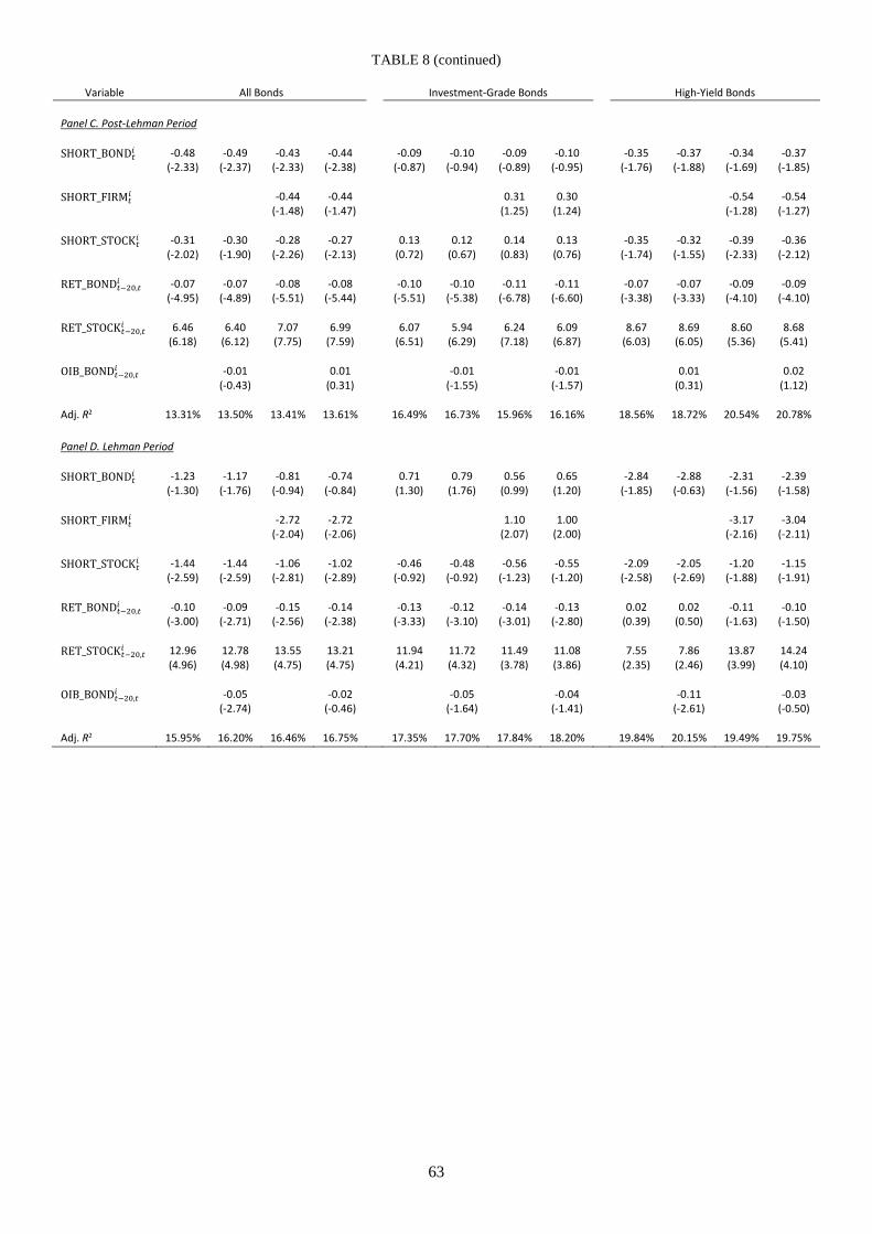
63

TABLE 8 (continued)


Panel C. Post-Lehman Period SHORT_BOND𝑡𝑡

𝑖𝑖 -0.48 (-2.33)

-0.49 (-2.37)

-0.43 (-2.33)

-0.44 (-2.38)

-0.09

(-0.87) -0.10

(-0.94) -0.09

(-0.89) -0.10

(-0.95)

-0.35

(-1.76) -0.37

(-1.88) -0.34

(-1.69) -0.37

(-1.85) SHORT_FIRM𝑡𝑡

𝑖𝑖

-0.44

(-1.48) -0.44

(-1.47)

0.31

(1.25) 0.30

(1.24)

-0.54

(-1.28) -0.54


𝑖𝑖 -0.31

(-2.02) -0.30

(-1.90) -0.28

(-2.26) -0.27

(-2.13)

0.13

(0.72) 0.12

(0.67) 0.14

(0.83) 0.13

(0.76)

-0.35

(-1.74) -0.32

(-1.55) -0.39

(-2.33) -0.36

(-2.12) RET_BOND𝑡𝑡−20,𝑡𝑡

𝑖𝑖 -0.07

(-4.95) -0.07

(-4.89) -0.08

(-5.51) -0.08

(-5.44)

-0.10

(-5.51) -0.10

(-5.38) -0.11

(-6.78) -0.11

(-6.60)

-0.07

(-3.38) -0.07

(-3.33) -0.09

(-4.10) -0.09

(-4.10) RET_STOCK𝑡𝑡−20,𝑡𝑡

𝑖𝑖 6.46 (6.18)

6.40 (6.12)

7.07 (7.75)

6.99 (7.59)

6.07

(6.51) 5.94

(6.29) 6.24

(7.18) 6.09

(6.87)

8.67

(6.03) 8.69

(6.05) 8.60

(5.36) 8.68

(5.41) OIB_BOND𝑡𝑡−20,𝑡𝑡

𝑖𝑖

-0.01 (-0.43)

0.01

(0.31)

-0.01

(-1.55)

-0.01

(-1.57)

0.01

(0.31)

0.02

(1.12) Adj. R2 13.31% 13.50% 13.41% 13.61%

16.49% 16.73% 15.96% 16.16%

18.56% 18.72% 20.54% 20.78%

Panel D. Lehman Period SHORT_BOND𝑡𝑡

𝑖𝑖 -1.23 (-1.30)

-1.17 (-1.76)

-0.81 (-0.94)

-0.74 (-0.84)

0.71

(1.30) 0.79

(1.76) 0.56

(0.99) 0.65

(1.20)

-2.84

(-1.85) -2.88

(-0.63) -2.31

(-1.56) -2.39

(-1.58) SHORT_FIRM𝑡𝑡

𝑖𝑖

-2.72

(-2.04) -2.72

(-2.06)

1.10

(2.07) 1.00

(2.00)

-3.17

(-2.16) -3.04


𝑖𝑖 -1.44

(-2.59) -1.44

(-2.59) -1.06

(-2.81) -1.02

(-2.89)

-0.46

(-0.92) -0.48

(-0.92) -0.56

(-1.23) -0.55

(-1.20)

-2.09

(-2.58) -2.05

(-2.69) -1.20

(-1.88) -1.15


𝑖𝑖 -0.10

(-3.00) -0.09

(-2.71) -0.15

(-2.56) -0.14

(-2.38)

-0.13

(-3.33) -0.12

(-3.10) -0.14

(-3.01) -0.13

(-2.80)

0.02

(0.39) 0.02

(0.50) -0.11

(-1.63) -0.10


𝑖𝑖 12.96 (4.96)

12.78 (4.98)

13.55 (4.75)

13.21 (4.75)

11.94 (4.21)

11.72 (4.32)

11.49 (3.78)

11.08 (3.86)

7.55

(2.35) 7.86

(2.46) 13.87 (3.99)

14.24 (4.10)

OIB_BOND𝑡𝑡−20,𝑡𝑡

𝑖𝑖

-0.05 (-2.74)

-0.02

(-0.46)

-0.05

(-1.64)

-0.04

(-1.41)

-0.11

(-2.61)

-0.03

(-0.50) Adj. R2 15.95% 16.20% 16.46% 16.75%

17.35% 17.70% 17.84% 18.20%

19.84% 20.15% 19.49% 19.75%

64

TABLE 9

Do Bond Short Sellers Have Information about Stock Returns? Cross-Sectional Regressions

Table 9 presents Fama–MacBeth (1973) regressions predicting 20-day stock abnormal returns. Each day we estimate the following cross-

sectional predictive regression:

RET_STOCK𝑡𝑡+2,𝑡𝑡+21𝑖𝑖

= 𝛼𝛼0𝑡𝑡 + 𝛼𝛼1𝑡𝑡SHORT_FIRM𝑡𝑡𝑖𝑖 + 𝛼𝛼2𝑡𝑡SHORT_STOCK𝑡𝑡

𝑖𝑖 + 𝛼𝛼3𝑡𝑡RET_STOCK𝑡𝑡−20,𝑡𝑡𝑖𝑖 + 𝛼𝛼4𝑡𝑡RET_BOND𝑡𝑡−20,𝑡𝑡

𝑖𝑖

+ 𝛼𝛼5𝑡𝑡OIB_STOCK𝑡𝑡−20,𝑡𝑡𝑖𝑖 + 𝛾𝛾𝑡𝑡𝑋𝑋𝑡𝑡𝑖𝑖 + 𝑢𝑢𝑡𝑡𝑖𝑖 .

We average then each coefficient over time-series dimension. The sample consists of all corporate bonds that have the corresponding stock

traded and have entries in the Markit securities lending database for which corresponding data is available in the FISD and TRACE

databases from Jan. 1, 2006 to Dec. 30, 2011. Stocks that are in the upper market capitalization quintile across the sample five days prior to

the sorting are categorized as Large stocks; stocks that are in the lowest market capitalization quintile are categorized as Small stocks. Pre-

Lehman period (Panel B) consists of all trading days from Jan. 1, 2006 to May 31, 2008, the post-Lehman period (Panel C) is from Jan. 1,

2009 to Dec. 30, 2011 and the Lehman period (Panel D) is from Jun. 1, 2008 to Dec. 30, 2008. Dependent variable is a simple average of

abnormal stock returns over the future 20 days defined as a raw return minus the return from the corresponding size and book-to-market

matching portfolio (annualized and expressed in percentages); SHORT_FIRM𝑡𝑡𝑖𝑖 is an average value-weighted ratio of the daily number of

bonds on loan (shorted) for bond issue i on day t to the number of bonds outstanding for all bonds issued by the firm except bond i (in

percentages); SHORT_STOCK𝑡𝑡𝑖𝑖 is a ratio of the daily number of shares on loan (shorted) for stock corresponding to bond issue i on day t to

a number of shares outstanding (in percentages); RET_BOND𝑡𝑡−20,𝑡𝑡𝑖𝑖 is a simple average of abnormal returns on bond i over the past 20 days

(in percentages); RET_STOCK𝑡𝑡−20,𝑡𝑡𝑖𝑖 is a simple average of abnormal returns on stock corresponding to bond issue i over the past 20 days

(in percentages); OIB_STOCK𝑡𝑡−20,𝑡𝑡𝑖𝑖 is a simple average over past 20 days of a trade imbalance of stock i defined as daily difference

between buy and sell trading volumes scaled by the total trading volume of the stock (in percentages). Control variables 𝑋𝑋𝑡𝑡𝑖𝑖 include:

VOLAT_STOCK𝑡𝑡−20,𝑡𝑡𝑖𝑖 is defined as a sum of absolute daily returns on stock i over the past 20 days (annualized and expressed in

percentages); TURN_STOCK𝑡𝑡−20,𝑡𝑡𝑖𝑖 is total daily value of bonds of stock i traded scaled by the total number of shares outstanding (in

percentages); ln(PAR_DEBT𝑡𝑡𝑖𝑖) is the natural log value of market capitalization of the firm i (in USD dollars); BM𝑡𝑡𝑖𝑖 is book-to-market ratio;

LEVERAGE𝑡𝑡𝑖𝑖 is defined as the sum of long-term and short-term debts divided by stockholders total equity; IHOLDING𝑡𝑡𝑖𝑖 institutional holding

is defined as the number of shares held by institutional investors as recorded in 13F filings and are scaled by the total number of shares

outstanding (in percentages). The t-statistics are reported in parentheses are based on the time series of coefficient estimates from the cross-

sectional regressions using Newey–West (1987) with 20 lags.

65

TABLE 9 (continued)

Variable All Stocks Small Stocks Large Stocks



0.24 (0.45)

0.10 (0.20)

0.25 (0.49)

0.29 (0.60)

-0.37

(-0.16) -0.63

(-0.28) -0.46

(-0.19) -0.80

(-0.35)

0.03

(0.06) -0.02

(-0.04) 0.09

(0.17) 0.23

(0.43) SHORT_STOCK𝑡𝑡

𝑖𝑖

-0.75

(-2.21) -0.79

(-2.29)

0.12

(0.18) 0.16

(0.24)

-1.41

(-2.53) -1.44


𝑖𝑖 0.01

(0.56) 0.01

(0.94) 0.01

(0.84) 0.01

(0.82)

0.02

(0.73) 0.03

(1.36) 0.02

(0.96) 0.03

(1.27)

0.00

(0.01) 0.00

(0.10) 0.00

(0.17) 0.00

(0.03) RET_BOND𝑡𝑡−20,𝑡𝑡

𝑖𝑖 -0.01 (-0.11)

-0.01 (-0.18)

-0.01 (-0.12)

-0.01 (-0.15)

-0.01

(-0.10) -0.03

(-0.26) -0.05

(-0.45) -0.06

(-0.56)

-0.01

(-0.33) -0.01

(-0.46) 0.00

(0.06) -0.00

(-0.08) OIB_STOCK𝑡𝑡−20,𝑡𝑡

𝑖𝑖

-0.09 (-0.34)

-0.13

(-0.49)

0.22

(0.26)

0.53

(0.66)

0.56

(1.74)

0.51

(1.59) Adj. R2 7.13% 7.33% 7.66% 7.87%

13.84% 14.86% 15.12% 15.79%

8.68% 8.85% 9.32% 9.51%



-0.04 (-0.05)

-0.18 (-0.20)

-0.11 (-0.13)

-0.24 (-0.29)

-0.39

(-0.09) -1.13

(-0.27) -0.45

(-0.10) -1.33

(-0.31)

-0.51

(-0.57) -0.50

(-0.56) -0.50

(-0.56) -0.48

(-0.54)


-0.29

(-0.66) -0.26

(-0.60)

0.38

(0.38) 0.43

(0.46)

-1.25

(-2.50) -1.22


𝑖𝑖 -0.02

(-1.64) -0.02

(-1.27) -0.02

(-1.43) -0.02

(-1.25)

-0.02

(-0.62) 0.02

(0.54) -0.01

(-0.20) 0.01

(0.42)

-0.02

(-1.50) -0.02

(-1.55) -0.02

(-1.26) -0.02


𝑖𝑖 0.01 (0.43)

0.01 (0.33)

0.01 (0.44)

0.01 (0.36)

-0.08

(-0.49) -0.06

(-0.37) -0.11

(-0.67) -0.09

(-0.54)

0.04

(1.07) 0.04

(1.05) 0.04

(1.19) 0.04

(1.16) OIB_STOCK𝑡𝑡−20,𝑡𝑡

𝑖𝑖

-0.30 (-0.71)

-0.30

(-0.74)

-1.56

(-1.36)

-1.21

(-1.11)

0.73

(1.65)

0.66

(1.49) Adj. R2 6.67% 6.91% 7.13% 7.37%

11.66% 12.62% 12.40% 12.92%

8.33% 8.33% 8.67% 8.71%

66

TABLE 9 (continued)

Variable All Stocks Small Stocks Large Stocks

Panel C. Post-Lehman Period SHORT_FIRM𝑡𝑡

𝑖𝑖 0.47

(1.37) 0.27

(0.65) 0.39

(1.14) 0.68

(1.81)

-0.01

(-0.01) 0.14

(0.12) -0.35

(-0.27) -0.21

(-0.17)

0.38

(1.44) 0.18

(0.52) 0.30

(1.13) 0.59

(1.83) SHORT_STOCK𝑡𝑡

𝑖𝑖

-0.75

(-2.29) -0.93

(-2.44)

-0.04

(-0.02) 0.12

(0.07)

-1.16

(-1.89) -1.26


𝑖𝑖 0.03

(1.72) 0.04

(1.98) 0.04

(1.91) 0.03

(1.73)

0.07

(1.76) 0.06

(1.60) 0.07

(1.76) 0.06

(1.63)

0.01

(0.41) 0.02

(0.56) 0.01

(0.49) 0.01

(0.31) RET_BOND𝑡𝑡−20,𝑡𝑡

𝑖𝑖 0.01 (0.30)

0.01 (0.30)

0.01 (0.40)

0.01 (0.42)

0.12

(0.97) 0.06

(0.49) 0.06

(0.51) 0.01

(0.11)

-0.07

(-1.52) -0.08

(-1.72) -0.05

(-1.18) -0.06

(-1.38) OIB_STOCK𝑡𝑡−20,𝑡𝑡

𝑖𝑖

0.17 (0.64)

0.08

(0.29)

2.66

(2.35)

2.78

(2.60)

0.34

(0.80)

0.26

(0.60) Adj. R2 6.34% 6.49% 6.77% 6.96%

16.09% 17.25% 18.44% 19.37%

7.81% 8.30% 8.50% 8.99%



0.89

(0.51) 0.99

(0.59) 1.69

(1.11) 1.75

(1.18) -1.77

(-0.52) -0.96

(-0.28) -0.94

(-0.29) -0.27

(-0.08) 1.67

(0.68) 1.83

(0.76) 2.63

(1.25) 2.81

(1.36)


-3.68 (-1.68)

-3.20 (-1.64)

-2.68 (-1.03)

-2.26 (-0.93)

-3.32 (-0.99)

-3.33 (-0.99)

RET_STOCK𝑡𝑡−20,𝑡𝑡𝑖𝑖

0.04

(0.71) 0.04

(0.71) 0.04

(0.86) 0.04

(0.85) -0.01

(-0.10) -0.01

(-0.15) -0.00

(-0.03) -0.01

(-0.14) 0.07

(0.90) 0.07

(0.92) 0.07

(1.02) 0.07

(1.05)

RET_BOND𝑡𝑡−20,𝑡𝑡𝑖𝑖 -0.13

(-1.53) -0.13

(-1.51) -0.15

(-1.65) -0.15

(-1.63) -0.12

(-0.37) -0.17

(-0.56) -0.11

(-0.33) -0.15

(-0.47) -0.01

(-0.18) -0.01

(-0.18) 0.00

(0.05) 0.01

(0.06)

OIB_STOCK𝑡𝑡−20,𝑡𝑡𝑖𝑖 -0.03

(-0.03) -0.06 (-0.05)

0.38 (0.11) 1.27

(0.36) 0.41

(0.32) 0.60 (0.48)

Adj. R2 13.33% 13.41% 14.60% 14.67% 17.27% 18.10% 17.19% 17.60% 14.53% 14.30% 16.70% 16.47%

67

TABLE 10

Substitution Effect in Short Selling around the Short Sale Ban

Table 10 presents a diff-in-diff analysis of the difference in short bond and stock interest, the difference in net new short interest

of bonds and stocks, and the difference in bond and stock lending fees around stock short sale ban. The sample consists of all

corporate bonds that have the corresponding stock traded, have entries in the Markit securities lending database for which

corresponding data is available in the FISD and TRACE databases from Aug. 1, 2008 to Oct. 7, 2008. We further merge this

sample with a list of firms which stocks were banned from short selling short sale ban period between Sept. 19, 2008 and Oct. 7,

2008. Our final sample consists of 117 banned firms and 824 non-banned firms. Specifically we estimate the following

regression:

𝑌𝑌𝑡𝑡𝑖𝑖 = 𝛼𝛼0 + 𝛼𝛼1BAN𝑡𝑡 + 𝛼𝛼2EVENT𝑖𝑖 + 𝛼𝛼3BAN𝑡𝑡 × EVENT𝑖𝑖 + 𝑢𝑢𝑡𝑡𝑖𝑖 ,

where 𝑌𝑌𝑡𝑡𝑖𝑖 corresponds to one of the following three variables: DIFF_SHORT𝑡𝑡𝑖𝑖 = SHORT_FIRM𝑡𝑡𝑖𝑖 − SHORT_STOCK𝑡𝑡

𝑖𝑖 is the

difference between stock and bond shorting for firm i and day t; DIFF∆SHORT𝑡𝑡𝑖𝑖 = ∆SHORT_FIRMti − ∆SHORT_STOCK𝑡𝑡

𝑖𝑖 is the

difference between net new short interest; DIFF_FEE𝑡𝑡𝑖𝑖 = LENDING_FEE_FIRM𝑡𝑡𝑖𝑖 − LENDING_FEE_STOCK𝑡𝑡

𝑖𝑖 . We define

SHORT_FIRM𝑡𝑡𝑖𝑖 as an average value-weighted ratio of the daily number of bonds on loan (shorted) for bond issue i on day t to

the number of bonds outstanding for all bonds issued by the firm except bond i (in percentages); SHORT_STOCK𝑡𝑡𝑖𝑖 is a ratio of

the daily number of shares on loan (shorted) for stock corresponding to bond issue i on day t to a number of shares outstanding

(in percentages); net new short interest ∆SHORT_FIRM𝑡𝑡𝑖𝑖 and ∆SHORT_STOCK𝑡𝑡

𝑖𝑖 are defined as the first differences in short

interest scaled by daily total trading volumes in bonds and stocks respectively; LENDING_FEE_STOCK𝑡𝑡𝑖𝑖 is defined as the

interest rate on cash funds minus the rebate rate for borrowing stock i (in basis points); LENDING_FEE_FIRM𝑡𝑡𝑖𝑖 is an average

value-weighted ratio of the bond lending fees for each bond issued by the firm i on day t (in basis points); EVENT𝑖𝑖 is a dummy

variable equal to 1 if the corresponding stock of firm i was banned from short selling by SEC between Sept. 19, 2008 and Oct.

7, 2008 and 0 otherwise; BAN𝑡𝑡 is a dummy variable equals to 1 if t is between Sept. 19, 2008 and Oct. 7, 2008 and 0 otherwise.

The t-statistics are reported in parentheses.

VARIABLE DIFF_SHORT𝑡𝑡𝑖𝑖 DIFF∆SHORT𝑡𝑡𝑖𝑖 DIFF_FEE𝑡𝑡𝑖𝑖 BAN𝑡𝑡 0.007 (0.06) 0.046 (4.71) 16.252 (2.90) EVENT𝑖𝑖 0.173 (0.79) -0.016 (-1.14) 29.413 (3.56) 𝐵𝐵𝐵𝐵𝐵𝐵𝑡𝑡 × EVENT𝑖𝑖 0.792 (2.46) 0.080 (3.01) 70.931 (4.70) INTERCEPT -5.847 (-91.8) 0.002 (0.46) -30.352 (-9.82) Adj. R2 0.03% 0.14% 0.49%

68

TABLE 11

Predicting Bond Short Interest: Cross-Sectional Regressions

Table 11 presents Fama–MacBeth (1973) regressions of predicting 5-day bond short interest. Each day we estimate the following cross-

sectional regression:

SHORT_BOND𝑡𝑡+2,𝑡𝑡+6𝑖𝑖

= 𝛼𝛼0𝑡𝑡 + 𝛼𝛼1𝑡𝑡RET_BOND𝑡𝑡−5,𝑡𝑡high + 𝛼𝛼2𝑡𝑡RET_BOND𝑡𝑡−5,𝑡𝑡

low + 𝛼𝛼3𝑡𝑡OIB_BOND𝑡𝑡−5,𝑡𝑡𝑖𝑖 + 𝛼𝛼4𝑡𝑡VOLAT_BOND𝑡𝑡−5,𝑡𝑡

𝑖𝑖

+ 𝛼𝛼5𝑡𝑡TURN_BOND𝑡𝑡−5,𝑡𝑡𝑖𝑖 + 𝛼𝛼6𝑡𝑡ln(PAR_DEBT𝑡𝑡𝑖𝑖) + 𝛼𝛼7𝑡𝑡SHORT_BOND𝑡𝑡−5,𝑡𝑡

𝑖𝑖 + 𝛼𝛼8𝑡𝑡SHORT_FIRM𝑡𝑡−5,𝑡𝑡𝑖𝑖 + 𝑢𝑢𝑡𝑡𝑖𝑖 .

We average then each coefficient over time-series dimension. The sample consists of all corporate bonds in the Markit securities lending

database for which corresponding data is available in the FISD and TRACE databases and the issuer’s stock from Jan. 1, 2006 to Dec. 30,

2011. Bonds with Moody’s credit rating of “Baa-3” and higher five days prior to the sorting are categorized as Investment-Grade Bonds;

others are categorized as High-Yield Bonds. Pre-Lehman period (Panel B) consists of all trading days from Jan. 1, 2006 to May 31, 2008,

the post-Lehman period (Panel C) is from Jan. 1, 2009 to Dec. 30, 2011 and the Lehman period (Panel D) is from Jun. 1, 2008 to Dec. 30,

2008. Dependent variable SHORT_BOND𝑡𝑡+2,𝑡𝑡+6𝑖𝑖 is a simple average of bond short interest over the future 5 days defined a ratio of the daily

number of bonds on loan (shorted) for bond issue i on day t to the number of bonds outstanding (expressed in percentages). To define

RET_BOND𝑡𝑡−5,𝑡𝑡high and RET_BOND𝑡𝑡−5,𝑡𝑡

low variables, we sort bonds on day t into terciles based on RET_BOND𝑡𝑡−5,𝑡𝑡𝑖𝑖 , where RET_BOND𝑡𝑡−5,𝑡𝑡

𝑖𝑖 is a

simple average of abnormal returns on bond i over the past 5 days (in percentages). RET_BOND𝑡𝑡−5,𝑡𝑡high = 1 if the bond abnormal return over

the past 5 trading days falls into the highest tercile and RET_BOND𝑡𝑡−5,𝑡𝑡high = 0 otherwise. Similarly, RET_BOND𝑡𝑡−5,𝑡𝑡

low = 1 if the bond

abnormal return over the past 5 trading days falls into the lowest tercile and RET_BOND𝑡𝑡−5,5low = 0 otherwise; SHORT_FIRM𝑡𝑡−5,𝑡𝑡

𝑖𝑖 is simple

average over the past 5 days of an average value-weighted ratio of the daily number of bonds on loan (shorted) for bond issue i on day t to

the number of bonds outstanding for all bonds issued by the firm except bond i (in percentages); OIB_BOND𝑡𝑡−5,𝑡𝑡𝑖𝑖 is a simple average over

past and future 5 days of a trade imbalance of bond i defined as daily difference between buy and sell trading volumes scaled by the total

trading volume of the bond (in percentages); VOLAT_BOND𝑡𝑡−5,𝑡𝑡𝑖𝑖 is defined as a sum of absolute daily returns on bond i over the past and

future 5 days respectively (daily and expressed in percentages); TURN_BOND𝑡𝑡−5,𝑡𝑡𝑖𝑖 is total daily number of bonds of issue i traded scaled by

the total number of bonds outstanding (in percentages); ln(PAR_DEBT𝑡𝑡𝑖𝑖) is the natural log value of the total amount of bonds outstanding

for bond issue i (in USD dollars). The t-statistics are reported in parentheses are based on the time series of coefficient estimates from the

cross-sectional regressions using Newey–West (1987) with 20 lags.

69

TABLE 11 (continued)


Panel A. Full Sample RET_BOND𝑡𝑡−5,𝑡𝑡

high 0.023 (5.78) 0.024 (5.79) 0.017 (2.52)

RET_BOND𝑡𝑡−5,𝑡𝑡low 0.020 (4.72) 0.013 (2.77) 0.027 (4.03)

OIB_BOND𝑡𝑡−5,𝑡𝑡𝑖𝑖 0.244 (39.4) 0.216 (32.0) 0.347 (38.0)

VOLAT_BOND𝑡𝑡−5,𝑡𝑡𝑖𝑖 -0.320 (-0.65) 0.654 (1.12) -1.304 (-1.49)

TURN_BOND𝑡𝑡−5,𝑡𝑡𝑖𝑖 1.133 (2.84) 0.993 (2.46) 3.539 (3.26)

ln(PAR_DEBT𝑡𝑡𝑖𝑖) 1.241 (4.24) 1.437 (4.14) 1.655 (3.77)

SHORT_BOND𝑡𝑡−5,𝑡𝑡𝑖𝑖 0.960 (211.4) 0.957 (175.2) 0.962 (232.2)

SHORT_FIRM𝑡𝑡−5,𝑡𝑡𝑖𝑖 0.011 (7.51) 0.009 (4.69) 0.009 (4.13)

Adj. R2 91.61% 90.82% 92.95%

Panel B. Pre-Lehman RET_BOND𝑡𝑡−5,𝑡𝑡

high 0.013 (1.80) 0.013 (1.92) 0.004 (0.35)

RET_BOND𝑡𝑡−5,𝑡𝑡low 0.031 (4.17) 0.025 (3.09) 0.043 (3.67)

OIB_BOND𝑡𝑡−5,𝑡𝑡𝑖𝑖 0.227 (29.83) 0.187 (21.3) 0.369 (31.6)

VOLAT_BOND𝑡𝑡−5,𝑡𝑡𝑖𝑖 -0.627 (-0.56) 0.762 (0.60) -2.118 (-1.05)

TURN_BOND𝑡𝑡−5,𝑡𝑡𝑖𝑖 1.523 (3.45) 1.176 (3.29) 4.747 (2.79)

ln(PAR_DEBT𝑡𝑡𝑖𝑖) 0.264 (0.50) 0.128 (0.23) 1.254 (1.42)



Adj. R2 93.29% 93.32% 93.27%

70

TABLE 11 (continued)

Variable All Bonds Investment-Grade Bonds High Yield Bonds

Panel C. Post-Lehman Period RET_BOND𝑡𝑡−5,𝑡𝑡

high 0.031 (7.67) 0.033 (7.93) 0.031 (4.29)

RET_BOND𝑡𝑡−5,𝑡𝑡low 0.010 (3.37) 0.003 (0.93) 0.020 (2.58)

OIB_BOND𝑡𝑡−5,𝑡𝑡𝑖𝑖 0.269 (34.9) 0.249 (30.9) 0.343 (27.3)

VOLAT_BOND𝑡𝑡−5,𝑡𝑡𝑖𝑖 0.116 (0.56) 0.701 (1.61) -0.148 (-0.77)

TURN_BOND𝑡𝑡−5,𝑡𝑡𝑖𝑖 1.145 (1.68) 1.258 (1.75) 3.695 (2.46)

ln(PAR_DEBT𝑡𝑡𝑖𝑖) 1.587 (6.18) 1.818 (5.80) 2.089 (5.20)



Adj. R2 90.72% 89.66% 92.54%

Panel D. Lehman Period RET_BOND𝑡𝑡−5,𝑡𝑡

high 0.029 (1.68) 0.022 (1.07) -0.004 (-0.20)

RET_BOND𝑡𝑡−5,𝑡𝑡low 0.023 (0.96) 0.004 (0.19) -0.006 (-0.25)

OIB_BOND𝑡𝑡−5,𝑡𝑡𝑖𝑖 0.182 (11.1) 0.174 (12.6) 0.262 (8.40)

VOLAT_BOND𝑡𝑡−5,𝑡𝑡𝑖𝑖 -1.312 (-2.93) -0.146 (-0.45) -3.943 (-3.58)

TURN_BOND𝑡𝑡−5,𝑡𝑡𝑖𝑖 -0.857 (-0.92) -1.430 (-1.38) -3.31 (-1.40)

ln(PAR_DEBT𝑡𝑡𝑖𝑖) 4.061 (5.79) 5.688 (5.20) 1.135 (0.88)


SHORT_FIRM𝑡𝑡−5,𝑡𝑡𝑖𝑖 0.010 (2.19) -0.006 (-0.74) 0.012 (1.43)

Adj. R2 88.47% 85.22% 93.72%

71

FIGURE 1

Sample Size

Plot of number of bonds lent against calendar years. Bonds in the sample include all corporate

bonds in the Markit securities lending database for which corresponding data is available in the

FISD and TRACE databases.

0

2,000

4,000

6,000

8,000

2006 2007 2008 2009 2010 2011

Year

NU

mbe

r of B

onds

Len

t

72

FIGURE 2

Short Interest

Plot of short interest (SHORT_BOND𝑡𝑡𝑖𝑖 ) defined as value-weights average of ratios of the number

of bonds on loan (shorted) to the number of bonds outstanding (in percentages) against calendar

date. The sample consists of all corporate bonds in the Markit securities lending database for

which corresponding data is available in the FISD and TRACE databases from Jan. 1, 2006 to

Dec. 30, 2011. Bonds with Moody’s credit rating of “Baa3” and higher five days prior to the

sorting are categorized as Investment-Grade Bonds; others are categorized as High-Yield Bonds.

0.5%

1.0%

1.5%

2.0%

2.5%

3.0%

3.5%

2006 2007 2008 2009 2010 2011

Perc

ent

Year

Investment Grade Bonds

High-Yield Bonds

73

FIGURE 3

Costs: Lending Fees and Realized Spreads

Figure 3 plots lending fees (Graph A plots means and Graph B plots medians) and realized

spread (Graph C) against calendar date for Investment and High-Yield bonds. Lending fee is

average value-weighted (with respect to the loan quantity) lending fee is defined as the interest

rate on cash funds minus the rebate rate (annualized and in basis points); realized spread is

defined as daily average buy price minus sell price of the bond scaled by the mid-price of the two

last buy and sell transactions (in percentages). The sample consists of all corporate bonds in the

Markit securities lending database for which corresponding data is available in the FISD and

TRACE databases from Jan. 1, 2006 to Dec. 30, 2011. Bonds with Moody’s credit rating of

“Baa3” and higher five days prior to the sorting are categorized as Investment-Grade Bonds;

others are categorized as High-Yield Bonds.

Graph A. Lending Fees: Means

-20

0

20

40

60

80

2006 2007 2008 2009 2010 2011

Basis

Poi

nts

Year


High-Yield Bonds

74

FIGURE 3 (continued)

Graph B. Lending Fees: Medians

Graph C. Realized Spreads

0

5

10

15

20

2006 2007 2008 2009 2010 2011

Basis

Poi

nts

Year


High-Yield Bonds

0

50

100

150

200

250

300

350

2006 2007 2008 2009 2010 2011

Basis

Poi

nts

Year


High-Yield Bonds

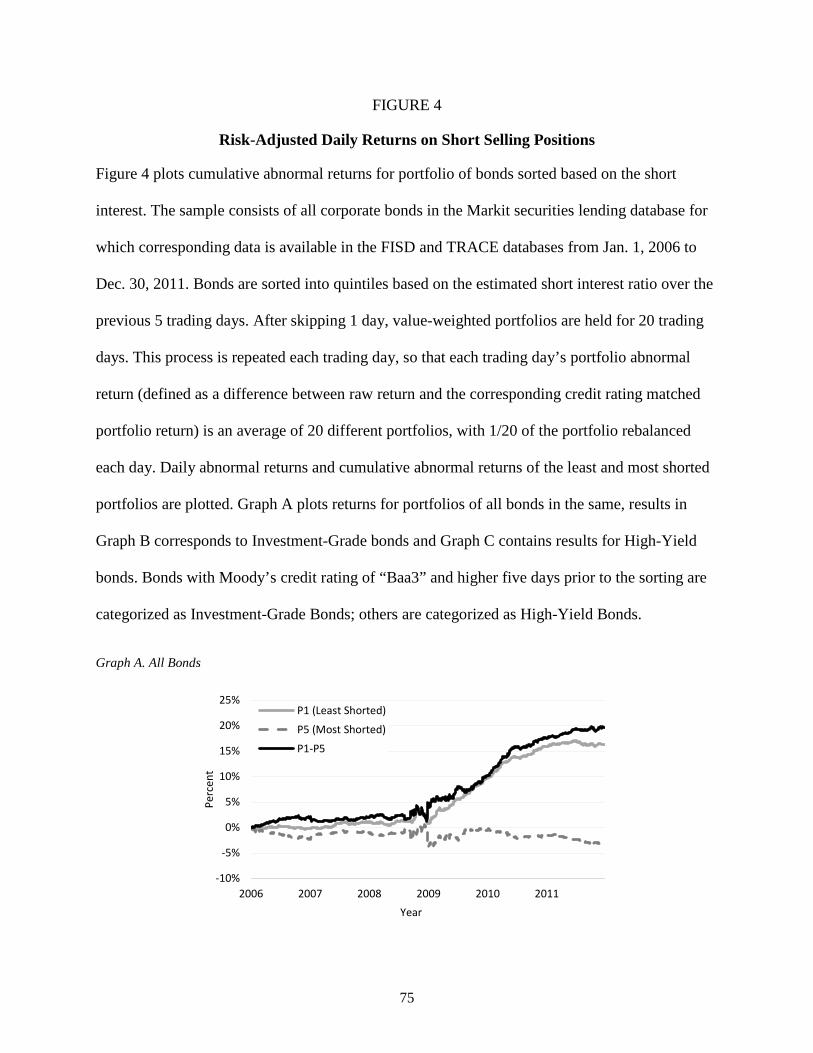
75

FIGURE 4

Risk-Adjusted Daily Returns on Short Selling Positions

Figure 4 plots cumulative abnormal returns for portfolio of bonds sorted based on the short

interest. The sample consists of all corporate bonds in the Markit securities lending database for

which corresponding data is available in the FISD and TRACE databases from Jan. 1, 2006 to

Dec. 30, 2011. Bonds are sorted into quintiles based on the estimated short interest ratio over the

previous 5 trading days. After skipping 1 day, value-weighted portfolios are held for 20 trading

days. This process is repeated each trading day, so that each trading day’s portfolio abnormal

return (defined as a difference between raw return and the corresponding credit rating matched

portfolio return) is an average of 20 different portfolios, with 1/20 of the portfolio rebalanced

each day. Daily abnormal returns and cumulative abnormal returns of the least and most shorted

portfolios are plotted. Graph A plots returns for portfolios of all bonds in the same, results in

Graph B corresponds to Investment-Grade bonds and Graph C contains results for High-Yield

bonds. Bonds with Moody’s credit rating of “Baa3” and higher five days prior to the sorting are

categorized as Investment-Grade Bonds; others are categorized as High-Yield Bonds.

Graph A. All Bonds

-10%

-5%

0%

5%

10%

15%

20%

25%

2006 2007 2008 2009 2010 2011

Perc

ent

Year

P1 (Least Shorted)

P5 (Most Shorted)

P1-P5

76


Graph B. Investment-Grade Bonds

Graph C. High-Yield Bonds

-10%

-5%

0%

5%

10%

15%

20%

25%

2006 2007 2008 2009 2010 2011

Perc

ent

Year

P1 (Least Shorted)P5 (Most Shorted)P1-P5

-60%

-40%

-20%

0%

20%

40%

60%

80%

100%

120%

2006 2007 2008 2009 2010 2011

Perc

ent

Year

P1 (Least Shorted)P5 (Most Shorted)P1-P5

77

FIGURE 5

Short Interest: Bonds versus Stocks

Plot of short interest for bonds and stocks matched sample. SHORT_BOND𝑡𝑡𝑖𝑖 defined as value-

weights average of ratios of the number of bonds on loan (shorted) to the number of bonds

outstanding (in percentages) against calendar date; SHORT_STOCK𝑡𝑡𝑖𝑖 defined as value-weights

average of ratios of the number of shares shorted to the number of shares outstanding (in

percentages) against calendar date. The sample consists of all corporate bonds in the Markit

securities lending database for which corresponding data is available in the FISD and TRACE

databases and corresponding stock data in CRSP from Jan. 1, 2006 to Dec. 30, 2011. Graph A

plots short interest for all bonds and stocks in matched sample, Graph B plots short interest for

small stocks and Graph C for large stocks. Small stocks correspond to the smallest quintile of

market size while large stocks are in the largest size quintile.

Graph A. Full Matched Sample of Bonds and Stocks

0%

2%

4%

6%

8%

10%

2006 2007 2008 2009 2010 2011

Perc

ent

Year

Bonds

Stocks

78


Graph B. Matched Sample of Small Stocks

Graph C. Matched Sample of Large Stocks

0%

2%

4%

6%

8%

10%

12%

14%

2006 2007 2008 2009 2010 2011

Perc

ent

Year

Bonds

Stocks

0.0%

0.5%

1.0%

1.5%

2.0%

2.5%

3.0%

3.5%

4.0%

2006 2007 2008 2009 2010 2011

Perc

ent

Year

Bonds

Stocks

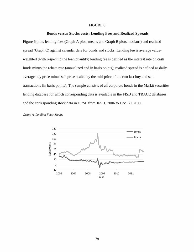
79

FIGURE 6

Bonds versus Stocks costs: Lending Fees and Realized Spreads

Figure 6 plots lending fees (Graph A plots means and Graph B plots medians) and realized

spread (Graph C) against calendar date for bonds and stocks. Lending fee is average value-

weighted (with respect to the loan quantity) lending fee is defined as the interest rate on cash

funds minus the rebate rate (annualized and in basis points); realized spread is defined as daily

average buy price minus sell price scaled by the mid-price of the two last buy and sell

transactions (in basis points). The sample consists of all corporate bonds in the Markit securities

lending database for which corresponding data is available in the FISD and TRACE databases

and the corresponding stock data in CRSP from Jan. 1, 2006 to Dec. 30, 2011.

Graph A. Lending Fees: Means

-20

0

20

40

60

80

100

120

140

2006 2007 2008 2009 2010 2011

Basis

Poi

nts

Year

Bonds

Stocks

80


Graph B. Lending Fees: Medians

Graph C. Realized Spreads

0

5

10

15

20

25

30

35

2006 2007 2008 2009 2010 2011

Basis

Poi

nts

Year

BondsStocks

0

2

4

6

8

10

12

0

50

100

150

200

250

300

2006 2007 2008 2009 2010 2011

Basis

Poi

nts

Basis

Poi

nts

Year

Bonds (left axis)

Stocks (right axis)

short selling and price discovery in corporate bonds

Documents