short circuit study of a balanced 3 phase system using p

Short Circuit Study of a Balanced 3 Phase System

Using p-inverse

A Thesis submitted to the

Dept. of Electrical & Electronics Engineering, BRAC University

in partial fulfillment of the requirements for the

Bachelor of Science degree in Electrical & Electronics Engineering

Hasan MuhommodSabbir

Md. Imam Hossain Rashed

Advisor: Amina Hasan Abedin

April 2015

2 | P a g e

Declaration

We to hereby declare that the thesis titled "Short Circuit Study of a Balanced 3 Phase

System using p-inverse function" is submitted to the Department of Electrical & Electronics

Engineering of BRAC University in partial fulfillment of the Bachelor of Science in Electrical &

Electronics Engineering. This is our original work and was not submitted elsewhere for the

award of any other degree or any other publications.

_______________________

Amina Hasan Abedin

(Thesis Supervisor)

Date:

_______________________


09221030

_______________________


09221031

3 | P a g e

Acknowledgement

We have benefited a lot from this thesis work. This project has been a rewarding

knowledge. We have learnt various aspects of power system analysis, power system structure

and also fault analysis by studying various papers, books, notes as well as internet.

We take this opportunity to acknowledge invaluable assistance of those people who

helped us in successful completion of this project and also express our special thanks to Amina

Hasan Abedin (Assistant Professor) who provided us an opportunity with lots of helpful

suggestions and format of making this thesis report.

Last but not list we express our thanks to all person and friends who always encourage us

and provide us support at all times.



4 | P a g e

Table of Contents

Declaration.................................................................................................. ................................................2

Acknowledgement......................................................................................................................................3

List of figures................................................................................ ..............................................................5

Abstract........................................................................................................................................................6

Chapter 1: Introduction............................................................................................................................7-21

1.1 Background........................................................................................................7

1.2 Why short circuit analyses.................................................................................8

1.2.1. Benefits of a Short Circuit Analysis.............................................9

1.3 Literature Review-Power Flow...........................................................................9

1.3.1 Power-flow problem formulation.................................................10

1.3.1.1 Newton–Raphson solution method..........................11

1.3.1.2 Gauss–Seidel method...............................................12

1.3.1.3 Fast-decoupled-load-flow method............................14

1.3.1.4 Holomorphic embedding load flow method.............14

1.4 Literature of Fault................................................................................... ............12

1.4.1 Types of Faults........................................................................ .......16

1.4.1.1 Transient fault...........................................................16

1.4.1.2 Persistent fault...........................................................16

1.4.1.3 Symmetric fault.........................................................17

1.4.1.4 Asymmetric fault.......................................................17

1.4.1.5 Bolted fault................................................................17

1.4.1.6 Realistic faults...........................................................18

1.4.1.7 Arcing fault...............................................................18

1.4.2 Transmission line fault...................................................................19

1.5 Objectives of Project............................................................................... .............21

Chapter 2: Methodology........................................................................................................ .....................22-50

2.1 Balanced 3-phase short circuit Analysis............................................................22

2.1.1 Hand Calculation for 4 bus.............................................................26

2.1.2 Result of Hand Calculation.............................................................37

2.2 Matlab Implementation........................................................................... ............38

2.2.1 Data format......................................................................................38

2.2.2 Assumptions....................................................................................39

2.2.3 Major functions...................................................................... ........40

2.2.3.1 main.m.......................................................................40

2.2.3.2 BalancedFaultAnalysis..............................................41

2.2.3.3 buildYbus.m..............................................................46

2.2.3.4 complexRuseltValue..................................................47

2.3 Matlab Results.......................................................................................... ............48

2.3.1 original format.................................................................................48

2.3.2 Tabular format.................................................................................48

2.4 Flow chart of execution........................................................................................50

Chapter 3: Conclusion.................................................................................................................................51-54

3.1 Finale....................................................................................................................51

3.2 Shortcoming.........................................................................................................52

3.3 Scopes of Project..................................................................................................52

Reference.......................................................................................................................................................53-54

5 | P a g e

List of figures:

Chapter 1: Figure 1.4.2 Four different types of transmission fault

Chapter 2: Figure2.1(a )single line diagram of a three bus system

Figure 2.1 (b) shows the changes in network voltage

Figure 2.1.1 (a) shows creating a short circuit on bus 2

Figure 2.1.1 (b) shows inserting an additional -Vf voltage source

Figure 2.1.1 (c) shows all voltage sources except –Vf are set to zero

Figure 2.1.1 (d) shows the sum up of all impedance

Figure 2.1.1 (e) shows the impedances are converted to admittances

Figure 2.1.1 (f) shows admittance conversion result

Figure 2.4 Shows work flow project

List of Table:

Table2.4 a. Line data (inpute)

Table 2.4b : Fault current at faulted bus

Table 2.4c. Balanced 3 Phase Bus Voltages during fault in per unit

Table 2.4d . Balanced 3 Phase Bus Voltages during fault in per unit

6 | P a g e

Abstract

Power system fault analysis is the process of determining the bus voltages and line currents

during the occurrence of various types of faults. Faults on power systems can be divided into

three-phase balanced faults and unbalanced faults. Three types of unbalanced fault occurrence on

power system transmission lines are single line to ground faults, line to line faults, and double

line to ground faults. Fault studies are used to select and set the proper protective devices and

switchgears. The determination of the bus voltages and line currents is very important in the fault

analysis of power system. The process consists of various methods of mathematical calculation

which is difficult to perform by hand. The calculation can be easily done by computer which is

generated by a program developed using MATLAB. However, in the conventional short circuit

study there arise an error while doing Y-bus to Z-bus inversion for a big bus system. To

minimize the error, this paper provides a solution which is solved through MATLAB, using p-

inverse methodology.

7 | P a g e

Chapter - 1

INTRODUCTION

1.1 Background

This project is focusing on the development of a method for power system fault analysis using

MATLAB. Power system fault analysis is the process of determining the magnitude of voltages

and line currents during the occurrence of various types of faults. The magnitude of these

currents depends on the internal impedance of the generators plus the impedance of the

intervening circuit. It can be of the order of tens of thousands of amperes. Faults on power

systems can be divided into three-phase balanced faults and unbalanced faults. Three types of

unbalanced fault occurrence on power system transmission lines are single line-to-ground faults,

line-to-line faults, and double line-to-ground faults. The magnitude of the fault current must be

accurately calculated in order that mechanical and thermal stresses on equipment may be

estimated. Fault studies are used to select and set the proper protective devices and switchgears.

The determination of the bus voltages and line currents is very important in the fault analysis of

power system. The process consists of various methods of mathematical calculation which

includes loads of formula and matrix approach to determine the magnitude of the voltage and

current. Thecalculation may form a large rows and columns of matrix depending on the number

of busses. The calculation is possible when dealing with small number of busses. However, it is

difficult to perform by hand when dealing with large number of busses. We will discuss the

method of analysis in the methodology.

8 | P a g e

Hence, the development of this project will ease user to perform the calculations of fault analysis

despite encountering large number of buses with less errors. The calculation can be easily done

by computer which is generated by a program developed using MATLAB. The program will

simulate the input data keyed in by the user.

1.2 Short circuit analyses

Short Circuit analysis is required to ensure the existing and new equipment ratings are sufficient

at each point in the electrical system. A Short Circuit Analysis will help to ensure that equipment

are protected by establishing proper interrupting ratings of protective devices (e.g. circuit breaker

and fuses). If an electrical fault exceeds the interrupting rating of the protective device, the

consequences can be devastating. It can be a serious threat to human life and is capable of

causing injury, extensive equipment damage, and costly. On large systems, short circuit analysis

is required to determine both the switchgear ratings and the relay settings. No substation

equipment can be installed without knowledge of the complete short circuit values for the entire

power distribution system. The short circuit calculations must be maintained and periodically

updated to protect the equipment and the lives. It is not safe to assume that new equipment is

properly rated.

9 | P a g e

1.2.1 Benefits of a Short Circuit Analysis

Performing a Short Circuit Study provides the following benefits:

Reduces the risk a facility could face and help avoid catastrophic losses.

Increases the safety and reliability of the power system and related equipment.

Evaluates the application of protective devices and equipment.

Identifies problem areas in the system.

Identifies recommended solutions to existing problems.

1.3 Literature Review-Power Flow

Before entering to the fault analysis first, we need to keep in mind the power-flow study, or load-

flow study, which is a numerical analysis of the flow of electric power in an interconnected

system. A power-flow study usually uses simplified notation such as a one-line diagram and per-

unit system, and focuses on various aspects of AC power parameters, such as voltages, voltage

angles, real power and reactive power. It analyzes the power systems in normal steady-state

operation. Power-flow or load-flow studies are important for planning future expansion of power

systems as well as in determining the best operation of existing systems. Commercial power

systems are usually too complex to allow for hand solution of the power flow whereas special

10 | P a g e

purpose network analyzers were built digital computers replaced the analog methods with

numerical solutions.

In addition to a power-flow study, computer programs perform related calculations such as

short-circuit fault analysis, stability studies, unit commitment and economic dispatch. In

particular, some programs use linear programming to find the optimal power flow, the conditions

which give the lowest cost per kilowatt hour delivered.

1.3.1 Power-flow problem formulation

The objective of a power-flow study is to obtain complete voltage angle and magnitude

information for each bus in a power system for specified load and generator real power and

voltage conditions. Once this information is known, real and reactive power flow on each branch

as well as generator reactive power output can be analytically determined.

The solution to the power-flow problem begins with identifying the known and unknown

variables in the system. The known and unknown variables are dependent on the type of bus. A

bus without any generators connected to it is called a Load Bus. With one exception, a bus with

at least one generator connected to it is called a Generator Bus. The exception is one arbitrarily

selected bus that has a generator. This bus is referred to as the Slack Bus.

11 | P a g e

There are several methods for solving the power flow problem. They are as follows-

1.3.1.1 Newton–Raphson solution method

There are several different methods of solving the resulting nonlinear system of equations. The

most popular is known as the Newton–Raphson method. This method begins with initial guesses

of all unknown .variables (voltage magnitude and angles at Load Buses and voltage angles at

Generator Buses). Next, a Taylor Series is written, with the higher order terms ignored, for each

of the power balance equations included in the system of equations. The result is a linear system

of equations that can be expressed as:

where and are called the mismatch equations:

and is a matrix of partial derivatives known as a Jacobian:

12 | P a g e

The linearized system of equations is solved to determine the next guess (m + 1) of voltage

magnitude and angles based on:

The process continues until a stopping condition is met.

1.3.1.2 Gauss–Seidel method

This is the earliest devised method. It shows slower rates of convergence compared to other

iterative methods, but it uses very little memory and does not need to solve a matrix system. In

numerical linear algebra, the Gauss–Seidel method, also known as the Liebmann method or the

method of successive displacement, is an iterative method used to solve a linear system of

equations.

The Gauss–Seidel method is an iterative technique for solving a square system of n linear

equations with unknown x:

.

It is defined by the iteration

13 | P a g e

where the matrix A is decomposed into a lower triangular component , and a strictly upper

triangular component U: .In more detail, write out A, x and b in their

components:

Then the decomposition of A into its lower triangular component and its strictly upper triangular

component is given by:

The system of linear equations may be rewritten as:

The Gauss–Seidel method now solves the left hand side of this expression for x, using previous

value for x on the right hand side. Analytically, this may be written as:

However, by taking advantage of the triangular form of , the elements of x(k+1)

can be

computed sequentially using forward substitution:

14 | P a g e

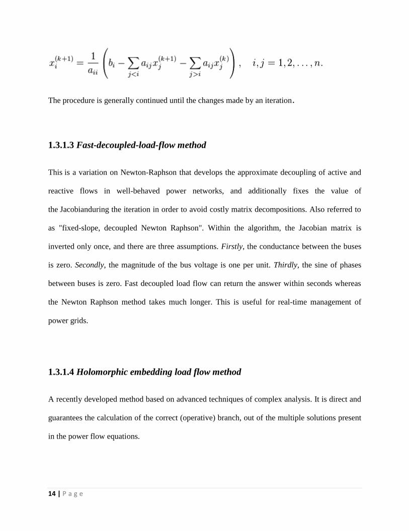
The procedure is generally continued until the changes made by an iteration.

1.3.1.3 Fast-decoupled-load-flow method

This is a variation on Newton-Raphson that develops the approximate decoupling of active and

reactive flows in well-behaved power networks, and additionally fixes the value of

the Jacobianduring the iteration in order to avoid costly matrix decompositions. Also referred to

as "fixed-slope, decoupled Newton Raphson". Within the algorithm, the Jacobian matrix is

inverted only once, and there are three assumptions. Firstly, the conductance between the buses

is zero. Secondly, the magnitude of the bus voltage is one per unit. Thirdly, the sine of phases

between buses is zero. Fast decoupled load flow can return the answer within seconds whereas

the Newton Raphson method takes much longer. This is useful for real-time management of

power grids.

1.3.1.4 Holomorphic embedding load flow method

A recently developed method based on advanced techniques of complex analysis. It is direct and

guarantees the calculation of the correct (operative) branch, out of the multiple solutions present

in the power flow equations.

15 | P a g e

A rough outline of solution of the power-flow problem is:

1. Make an initial guess of all unknown voltage magnitudes and angles. It is common to use

a "flat start" in which all voltage angles are set to zero and all voltage magnitudes are set

to 1.0 p.u.

2. Solve the power balance equations using the most recent voltage angle and magnitude

values.

3. Linearize the system around the most recent voltage angle and magnitude values

4. Solve for the change in voltage angle and magnitude

5. Update the voltage magnitude and angles

6. Check the stopping conditions, if met then terminate, else go to step 2.

1.4 LiteratureReview ofFault

In an electric power system, a fault is unusual electric current. A short circuit is also considered

as a fault in which current bypasses the normal load. An open-circuit fault occurs if a circuit is

interrupted by some failure. In three-phase systems, a fault may involve one or more phases and

ground, or may occur only between phases. In a "ground fault" or "earth fault", charge flows into

the earth. The prospective short circuit current of a fault can be calculated for power systems. In

power systems, protective devices detect fault conditions and operate circuit breakers and other

devices to limit the loss of service due to a failure.

16 | P a g e

1.4.1 Types of Faults

1.4.1.1 Transient fault

A transient fault is a fault that is no longer present if power is disconnected for a short time and

then restored. Many faults in overhead power lines are transient in nature. When a fault occurs,

equipment used for power system protection operate to isolate the area of the fault. A transient

fault will then clear and the power-line can be returned to service. Typical examples of transient

faults include:

Momentary tree contact

Bird or other animal contact

Lightning strike

Conductor clashing

1.4.1.2 Persistent fault

A persistent fault does not disappear when power is disconnected. Faults in

underground power cables are most often persistent due to mechanical damage to the cable, but

are sometimes transient in nature due to lightning.

17 | P a g e

1.4.1.3 Symmetric fault

A symmetric or balanced fault affects each of the three phases equally. In transmission line

faults, roughly 5% are symmetric. This is in contrast to an asymmetrical fault, where the three

phases are not affected equally.

1.4.1.4 Asymmetric fault

An asymmetric or unbalanced fault does not affect each of the three phases equally.

Common types of asymmetric faults, and their causes:

line-to-line - a short circuit between lines, caused by ionization of air, or when lines come into

physical contact, for example due to a broken insulator.

line-to-ground - a short circuit between one line and ground, very often caused by physical

contact, for example due to lightning or other storm damage

double line-to-ground - two lines come into contact with the ground also commonly due to storm

damage.

1.4.1.5 Bolted fault

One extreme is where the fault has zero impedance, giving the maximum prospective short-

circuit current. Notionally, all the conductors are considered connected to ground as if by a

metallic conductor; this is called a "bolted fault". It would be unusual in a well-designed power

18 | P a g e

system to have a metallic short circuit to ground but such faults can occur by mischance. In one

type of transmission line protection, a "bolted fault" is deliberately introduced to speed up

operation of protective devices.

1.4.1.6 Realistic faults

Realistically, the resistance in a fault can be from close to zero to fairly high. A large amount

of power may be consumed in the fault, compared with the zero-impedance case where the

power is zero. Also, arcs are highly non-linear, so a simple resistance is not a good model. All

possible cases need to be considered for a good analysis.

1.4.1.7 Arcing fault

Where the system voltage is high enough, an electric arc may form between power system

conductors and ground. Such an arc can have a relatively high impedance and can be difficult to

detect by simple over current protection. For example, an arc of several hundred amperes on a

circuit normally carrying a thousand amperes may not trip over current circuit breakers but can

do enormous damage to bus bars or cables before it becomes a complete short circuit. Utility,

industrial, and commercial power systems have additional protection devices to detect relatively

small but undesired currents escaping to ground. In residential wiring, electrical regulations may

now require Arc-fault circuit interrupters on building wiring circuits, to detect small arcs before

they cause damage or a fire.

19 | P a g e

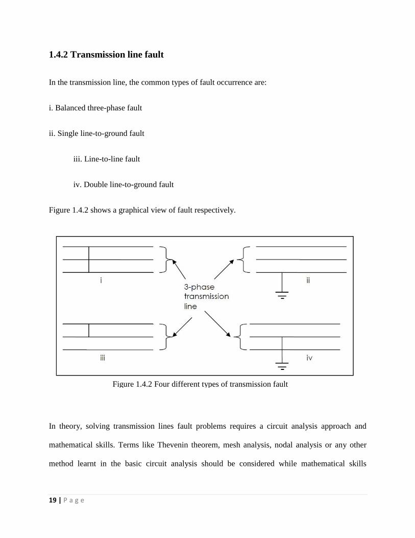
1.4.2 Transmission line fault

In the transmission line, the common types of fault occurrence are:

i. Balanced three-phase fault

ii. Single line-to-ground fault

iii. Line-to-line fault

iv. Double line-to-ground fault

Figure 1.4.2 shows a graphical view of fault respectively.

In theory, solving transmission lines fault problems requires a circuit analysis approach and

mathematical skills. Terms like Thevenin theorem, mesh analysis, nodal analysis or any other

method learnt in the basic circuit analysis should be considered while mathematical skills

Figure 1.4.2 Four different types of transmission fault

20 | P a g e

required for forming a Bus Impedance Matrix (Zbus) in order to put them in matrix outline. In

general, the analysis of any fault condition is performed in the following order:

i. Represent the given power system by its positive, negative and zero-sequence

networks. This representation requires the calculation of per unit (p.u.) impedances for

generators, transformers, lines, cables and other elements of the power system.

ii. Reduce each of the sequence networks to its simplest form. The equivalent positive,

negative and zero-sequence networks are represented as a series and series-parallel combinations

of the p.u. impedances. These are replaced by the single equivalent impedance for each sequence

network. It may also involve the use of the delta-star or star-delta transformations.

iii. Use the appropriate symmetrical-component equations to find the phase sequence

components of the current in fault under the particular short-circuit condition.

iv. Determine the required p.u. phase-current values at the point of fault.

v. Finally, calculate the actual values of the phase-currents by multiplying obtained p.u.

values by the base current at the point of fault.

The procedure outlined above provides a complete analysis of the given power system for the

specified fault condition and can be easily implemented in computer aided tutorials.

In a poly phase system, a fault may affect all phases equally which is known as "symmetrical

fault". If only some phases are affected, the situation is known as "asymmetrical fault." In real

power engineering world asymmetrical fault becomes more complicated to analyze due to the

simplifying assumption of equal current magnitude in all phases which is not longer applicable.

21 | P a g e

The analysis of this type of fault is often simplified by using methods such as symmetrical

components.

1.5 Objectives of Project

The objective of this project is to study the common fault type which is balance fault of the

transmission line in the power system. Secondly is to perform the analysis and obtain the results

from simulation on those types of fault using MATLAB. Lastly is to develop a toolbox for power

system fault analysis for educational and training purposes.

22 | P a g e

Chapter - 2

Fault Calculation

2.1 Balanced 3-phase short circuit Analysis

Theory

During a three-phase fault, the impedance of a generator is a time varying quantity. It is Xd" in

the sub-transient period (one to four cycles), Xd' in the transient period (about 30 cycles), and the

synchronous reactance Xd after that. The sub-transient currents can be very large due to the small

size of Xd". Due to symmetry, the three phase currents during a symmetrical fault can be solved

using ordinary circuit theory. In this case, Thevenin's theorem is being used for simple and small

power circuits only to analyze the fault. If the fault has zero impedance to ground, it is called a

solid fault or bolted fault (all three lines shorted to ground with zero impedance). However, it is

impractical for a real large power system. A systematic method is presented in this section which

applies to power systems of any size. The method can also be programmed on a computer shows

in figure 2.1 (a).

Figure2.1 (a) Single line diagram of a three bus system

23 | P a g e

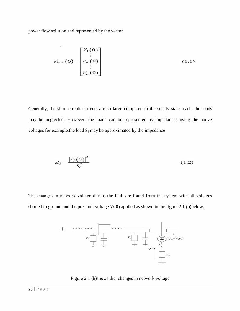
power flow solution and represented by the vector

Generally, the short circuit currents are so large compared to the steady state loads, the loads

may be neglected. However, the loads can be represented as impedances using the above

voltages for example,the load Si may be approximated by the impedance

The changes in network voltage due to the fault are found from the system with all voltages

shorted to ground and the pre-fault voltage Vk(0) applied as shown in the figure 2.1 (b)below:

Figure 2.1 (b)shows the changes in network voltage

24 | P a g e

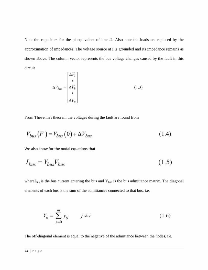
Note the capacitors for the pi equivalent of line ik. Also note the loads are replaced by the

approximation of impedances. The voltage source at i is grounded and its impedance remains as

shown above. The column vector represents the bus voltage changes caused by the fault in this

circuit

From Thevenin's theorem the voltages during the fault are found from

We also know for the nodal equations that

whereIbus is the bus current entering the bus and Ybus is the bus admittance matrix. The diagonal

elements of each bus is the sum of the admittances connected to that bus, i.e.

The off-diagonal element is equal to the negative of the admittance between the nodes, i.e.

25 | P a g e

whereyijis the actual admittance between nodes iand j. For the Thevenin circuit above,the nodal

equations are

Note that the minus sign is due to the fact the fault current is shown leaving node k. Theabove

matrix equation can be written as

which can be solved for the voltage change thus

whereZbus= Ybus-1

is known as the bus impedance matrix Using (1.10) in (1.4) we have:

Which can be expanded into matrix form:

26 | P a g e

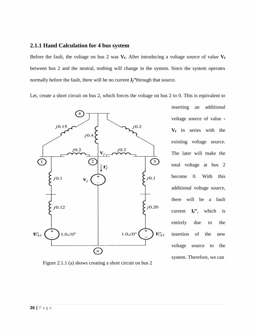
2.1.1 Hand Calculation for 4 bus system

Before the fault, the voltage on bus 2 was Vf. After introducing a voltage source of value Vf

between bus 2 and the neutral, nothing will change in the system. Since the system operates

normally before the fault, there will be no current If”through that source.

Let, create a short circuit on bus 2, which forces the voltage on bus 2 to 0. This is equivalent to

inserting an additional

voltage source of value -

Vf in series with the

existing voltage source.

The later will make the

total voltage at bus 2

become 0. With this

additional voltage source,

there will be a fault

current If”, which is

entirely due to the

insertion of the new

voltage source to the

system. Therefore, we can

Figure 2.1.1 (a) shows creating a short circuit on bus 2

27 | P a g e

use superposition to analyze the effects of the new voltage source on the system. The resulting

current If” will be the current for the entire power system, since the other sources in the system

produced a net zero current.

Figure 2.1.1 (b) shows inserting an additional -Vfvoltage source

28 | P a g e

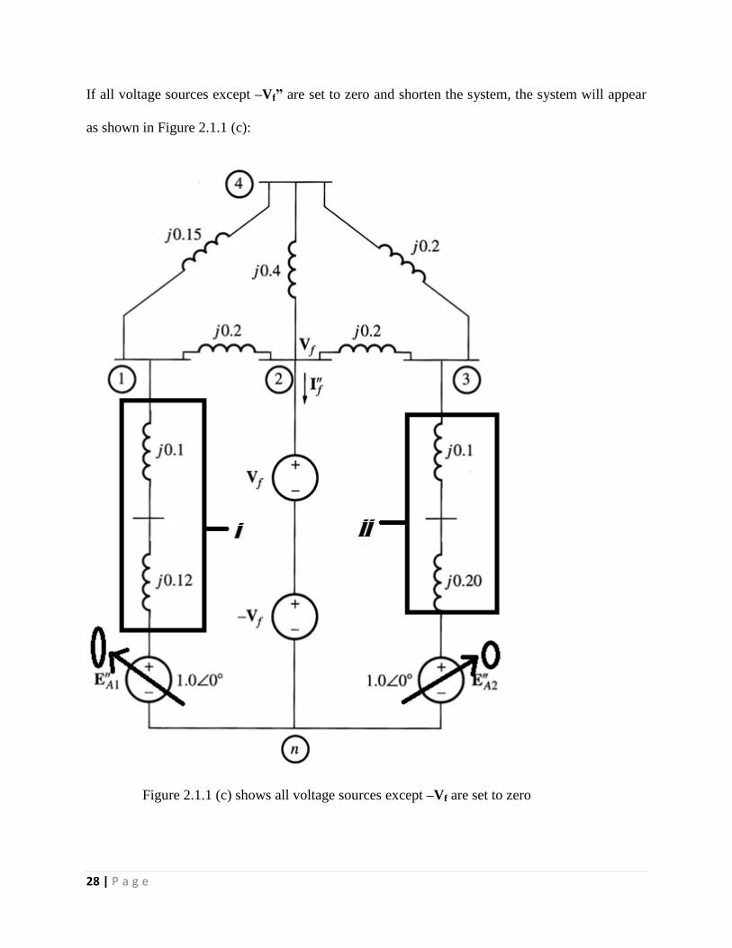
If all voltage sources except –Vf” are set to zero and shorten the system, the system will appear

as shown in Figure 2.1.1 (c):

Figure 2.1.1 (c) shows all voltage sources except –Vf are set to zero

29 | P a g e

i = j 0.1 + j 0.12 = j 0.22

ii = j 0.1 + j 0.20 = j 0.30

Figure 2.1.1 (d) shows the sum up of all impedance

30 | P a g e

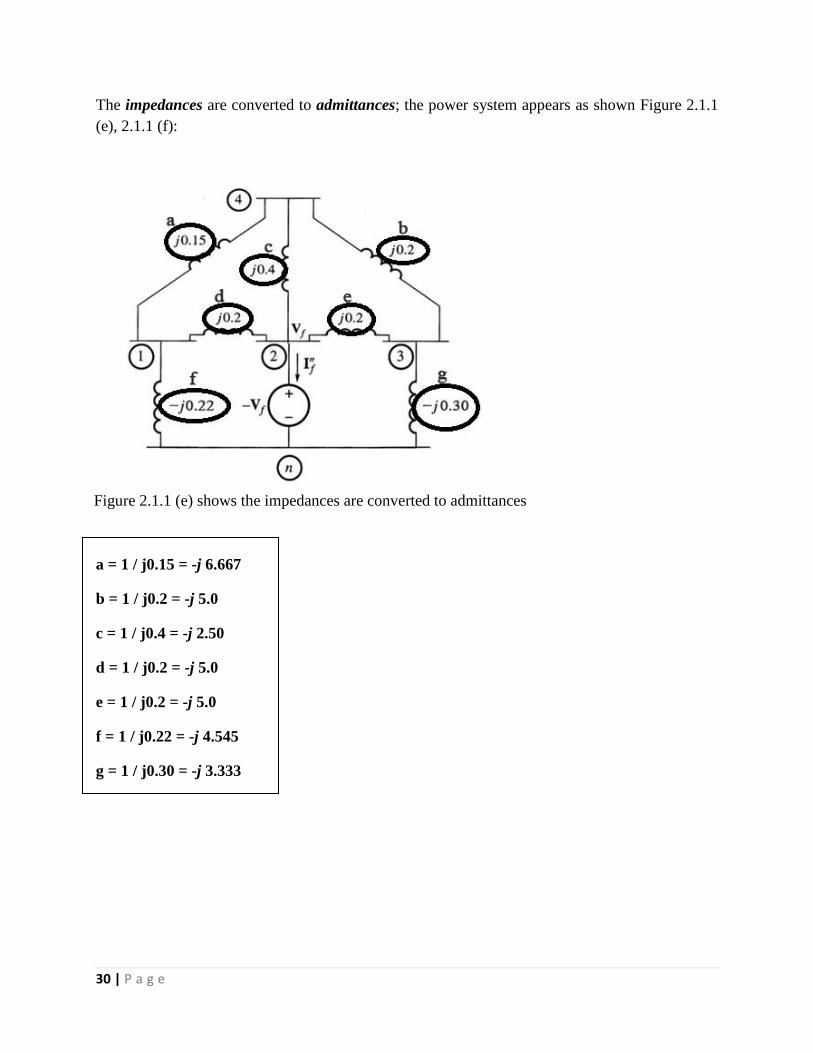
The impedances are converted to admittances; the power system appears as shown Figure 2.1.1

(e), 2.1.1 (f):

a = 1 / j0.15 = -j 6.667

b = 1 / j0.2 = -j 5.0

c = 1 / j0.4 = -j 2.50

d = 1 / j0.2 = -j 5.0

e = 1 / j0.2 = -j 5.0

f = 1 / j0.22 = -j 4.545

g = 1 / j0.30 = -j 3.333

Figure 2.1.1 (e) shows the impedances are converted to admittances

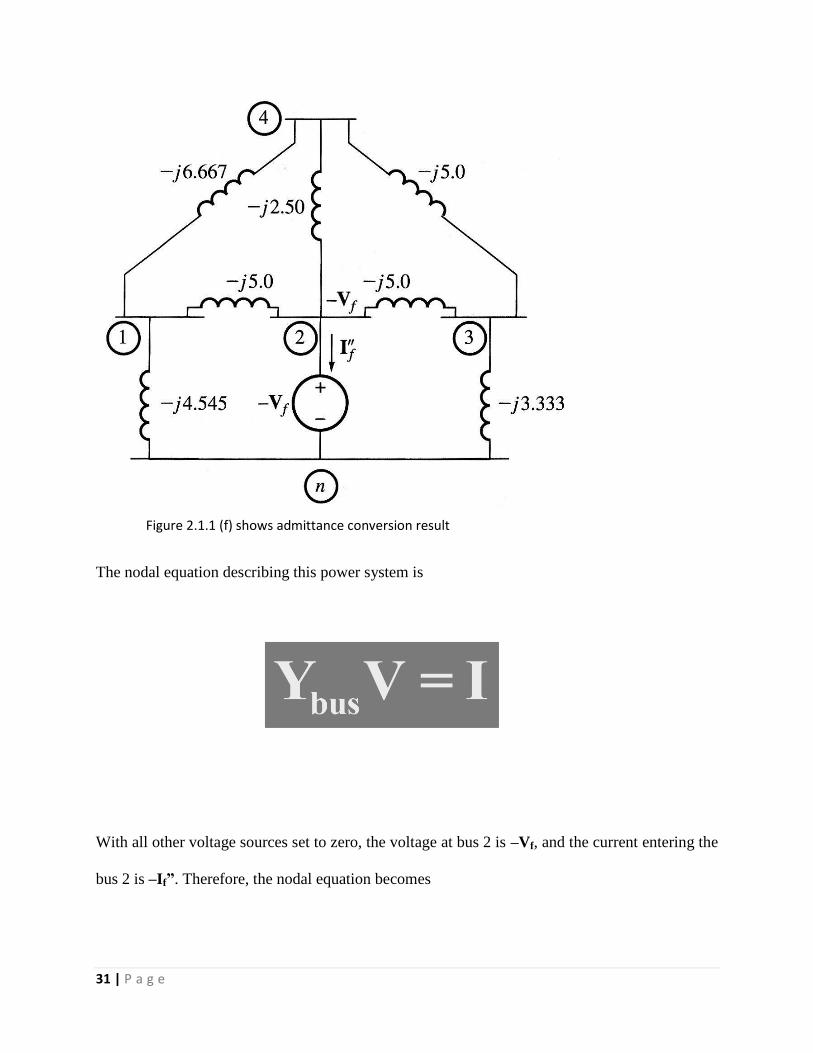
31 | P a g e

The nodal equation describing this power system is

With all other voltage sources set to zero, the voltage at bus 2 is –Vf, and the current entering the

bus 2 is –If”. Therefore, the nodal equation becomes

Figure 2.1.1 (f) shows admittance conversion result

32 | P a g e

Y11 = The Connection between Bus 1 and Bus 1










33 | P a g e







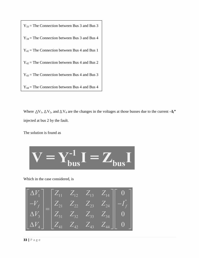
Where V1, V2, and V4 are the changes in the voltages at those busses due to the current –If”

injected at bus 2 by the fault.

The solution is found as

Which in the case considered, is

34 | P a g e

Where Zbus = Ybus-1

. Since only bus 2 has current injected at it, the system reduces to

Therefore, the fault current at bus 2 is just the prefault voltage Vf at bus 2 divided by Z22, the

driving point impedance at bus 2.

The voltage differences at each of the nodes due to the fault current can be calculated by

substitution:

35 | P a g e

Assuming that the power system was running at no load conditions before the fault, it is easy to

calculate the voltages at every bus during the fault. At no load, the voltage will be the same on

every bus in the power system, so the voltage on every bus in the system is Vf. The change in

voltage on every bus caused by the fault current –If”

For this system, the bus admittance matrix is constructed as follows:

36 | P a g e

Y11 = Y10 + Y12 + Y13 + Y14 = -j 4.545 - j 5.0 - 0 - j 6.667 = - j 16.212

Y12 = - Y12 = j 5.0

Y13 = 0

Y14 = - Y14 = j 6.667

Y21 = - Y21 = j 5.0

Y22 = Y20 + Y21 + Y23 + Y24 = 0 - j 5.0 - j 5.0 - 2.50 = -j 12.5

Y23 = - Y23 = j 5.0

Y24 = - Y24 = j 2.5

Y31 = 0

Y32 = - Y32 = j 5.0

Y33 = Y30 + Y31 + Y32 + Y34 = -j 3.333 - 0 - j 5.0 - j 5.0 = - j 13.333

Y34 = -Y34 = j 5.0

Y41 = -Y41 = j 6.667

Y42 = -Y42 = j 2.5

Y43 = -Y43 = j 5.0

Y44 = Y41 + Y42 + Y43 + Y40 = -j 6.667- j 2.50 - j 5.0 = - j 14.167

37 | P a g e

The bus impedance matrix calculated using Matlab as the inverse of Ybus is

2.1.2 Result of Hand Calculation

For the given power system, the no-load voltage at every bus is equal to the pre-fault voltage at

the bus that is

The current at the faulted bus is computed as

38 | P a g e

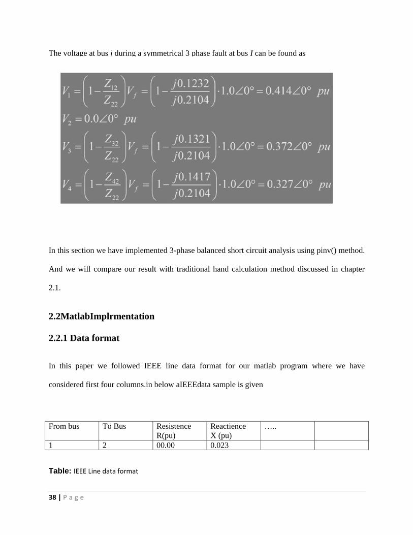
The voltage at bus j during a symmetrical 3 phase fault at bus I can be found as

2.2 Matlab Implementation

In this section we have implemented 3-phase balanced short circuit analysis using pinv() method.

And we will compare our result with traditional hand calculation method discussed in chapter

2.1.

2.2MatlabImplrmentation

2.2.1 Data format

In this paper we followed IEEE line data format for our matlab program where we have

considered first four columns.in below aIEEEdata sample is given

From bus To Bus Resistence

R(pu)

Reactience

X (pu)

…..

1 2 00.00 0.023

Table: IEEE Line data format

39 | P a g e

2.2.2 Assumptions

In This proposed method we have made some assumption .We neglected resistance from line

data as it has minimum effect and we used pre fault voltage as 1 per unit for calculation case.

The following assumptions are also made:

1. Shunt capacitances are neglected and the system is considered on no-load. 2.

2. All generators are running at their rated voltage and rated frequency with their emfs in

phase

40 | P a g e

2.2.3 Major functions

To solve this problem we have created as one main class and 3 functions

• main.m

• BalancedFaultAnalysis.m

• buildYbus.m

• complexRuseltValue

2.2.3.1 main.m

Our main program is main.mwherelindatawill be stored.Inmain.m class first it calculates [1]

maximum number of buses in the network. Here we assume the pre fault voltage (vo)[ 2]at each

buses as 1 per unit (pu) for calculation purpose. It can be taken from user or can be taken from

any power flow analysis prompt a GUI for take two inputs. First one is fault bus number

(fbusNo) and other one is fault Impedance zf .After taking inputs it convert the taken value

string to number and call our function BalancedFaultAnalysis().

lineData=[ 0 1 0 0.22 0 3 0 0.30 1 2 0 0.2 1 4 0 0.15 2 3 0 0.2 2 4 0 0.4 3 4 0 0.2 ];

%1 NumberofBuses = max(max (lineData(:,1)),max(lineData(:,2)));

fprintf('You have %d busse in your Network ',NumberofBuses); %2

41 | P a g e

preFaultVoltage=ones(NumberofBuses,1); % [~,~,~,~,~,Ybus]=buildYbus(lineData);

%GUI INPUT

prompt={'Enter your The Fault Bus No:','Enter fault impedence

(R+j*X) Zero for Bolted:'}; % Create all your text fields with the questions specified by

the variable prompt. title='3-Phase Balanced Short circuit Analysis '; % The main title of your input dialog interface. answer=inputdlg(prompt,title); % Convert these values to a number using str2num. fbusNo= str2num(answer{1}); zf = str2num(answer{2}); % % % zf=0; % fbusNo=4;

BalancedFaultAnalysis(lineData,preFaultVoltage,zf,fbusNo);

2.2.3.2 BalancedFaultAnalysis

This function takes four parameters lineData,preFaultVoltage,zf,fbusNoand it

does not return anything. When this function is called from main.m class that class will give it

all the four parameters it required to run. Then it calls buildYbus() and give it lineDataas

parameter and it returns Y-bus matrix (Ybus) and other data like

fromBus,toBus,NumberofBuses,NumberOfBranches,Z. After that it inverts

YbusintoZbususingpinv() method what is bult-in function of matlab. In next step it

calculates fault current of given fault bus [4] and printed in rectangular form and then convert it

42 | P a g e

into polar format. Then its Prompt a GUI for taking input for viewing [5] different types of

result. Input 1 for per unite polar form and 2 for rectangular form. Then it calculates fault

voltages of each buses [6] and prints the result according to user defined view mode. At last it

calculates and shows line to line current [7] after fault. It also invokedcomplexResultValue

() to view complex result format.

functionBalancedFaultAnalysis(lineData,V0,Zf,fbusNo)

%[3]

[fromBus,toBus,NumberofBuses,NumberOfBranches,Z,Ybus]=

buildYbus(lineData);

% making Zbus by Inverting Ybus

%yb=ybus4(lineData);

Zbus=inv(Ybus);

Ybus

Zbus=Zbus*(-1)

%Zbus=Zbus./(90.476/100);

%Calculating Fault-current

magVfault=0;

fprintf('Three-phase Balanced fault at bus No. %d\n\n\n ' ,

fbusNo)

%[4]

IfaultCurrent = (V0(fbusNo))/(Zf + Zbus(fbusNo, fbusNo));

%Inpufaultcurrent

Ifault_m = abs(IfaultCurrent);

Ifault_mang=angle(IfaultCurrent)*180/pi;

%disp(' ## 3-Phase Balanced Fault Current ## ')

fprintf('|---------------------------------------|\n')

IfaultCurrent

fprintf('|---------------------------------------|\n\n\n')

%in pu

FaultCurrentMag = abs(IfaultCurrent)

FaultCurrentAng=angle(IfaultCurrent)*180/pi

43 | P a g e

%[5]

%GUI for choosing result mood

prompt={'Enter 1 For per Unit Output 2 For Rectangle Form

Output'};

% % Create all your text fields with the questions specified by

the variable prompt.

title='3-Phase Balanced Short circuit Analysis ';

% % The main title of your input dialog interface.

answer=inputdlg(prompt,title);

% % Convert these values to a number using str2num.

viewMode= str2num(answer{1});

%viewMode =input('Enter 1 for per unint')

ifviewMode==1

% Start of 1st If

%preparing for printing results in pu

fprintf(' ##Balanced 3 Phase Bus Voltages during fault in per

unit \n\n')

fprintf(' |-------|---------------|--------------------|\n')

fprintf(' | Bus | Voltage | Voltage Angle |\n')

fprintf(' | No. | Magnitude | degrees |\n')

fprintf(' |-------|---------------|--------------------|\n')

else

%preparing for printing results in rectangler/complex form

fprintf(' ##Balanced 3 Phase Bus Voltages After fault \n\n')

fprintf(' |-------|---------------|--------------------|\n')

fprintf(' | Bus | Voltage | Voltage |\n')

fprintf(' | No. | MW | Mvr |\n')

fprintf(' |-------|---------------|--------------------|\n')

end%end of 1st if

%[6]

%calculating Vfault of each bus

for n = 1:NumberofBuses

%start of 1st For loop

if n==fbusNo

% at Fault Bus

Vfault(n) = (V0(fbusNo)*Zf )/(Zf + Zbus(fbusNo,fbusNo));

%converting topu

mVfault = abs(Vfault(n));

angVfault=angle(Vfault(n))*180/pi;

mVfaultReal=real(Vfault(n));

mVfaultImg=imag(Vfault(n));

44 | P a g e

else

%Vfault(n) = (V0(n)-(V0(n)*Zbus(n,fbusNo)))/(

Zbus(fbusNo,fbusNo) +Zf);

Vfault(n)= ( V0(n)-(Zbus(n,fbusNo)*IfaultCurrent));

end

%converting topu

magVfault = abs(Vfault(n));

angVfault=angle(Vfault(n))*180/pi;

mVfaultReal=real(Vfault(n));

mVfaultImg=imag(Vfault(n));

ifviewMode==1


fprintf(' %5g', n)

%fprintf(' |\n')

fprintf('%17.5f', magVfault)

%fprintf(' |')

fprintf(' %15.5f\n', angVfault)

% fprintf(' |')

fprintf(' |-------|---------------|--------------------|\n')

else


fprintf(' %4g', n)

%fprintf(' |\n')

fprintf('%17.4g', mVfaultReal)

%fprintf(' |')

fprintf(' %15.4g\n', mVfaultImg)

% fprintf(' |')

fprintf(' |-------|---------------|--------------------|\n')

end

end%End of 1st for loop

% calculating Line_to Line Current

fprintf('\n\n')


ifviewMode==1

disp(' ## 3-Phase Balanced Line-to-Line Fault

Curren ## ')

disp(' |------------------------------------------------------

----------------|')

disp(' | Bus | Bus | current |

Current Angle |')

45 | P a g e

disp(' | to. | from | Magnitude |

degrees |')

disp(' |------------------------------------------------------

----------------|')

else


disp(' ## 3-Phase Balanced Line-to-Line Fault

Curren ## ')

disp(' |------------------------------------------------------

----------------|')

disp(' | Bus | Bus | current |

Current Angle |')

disp(' | to. | from | Real |

Imagenary |')

disp(' |------------------------------------------------------

----------------|')

end

%[7]

fori=1:NumberOfBranches

iftoBus(i)>0 &&fromBus(i)>0

IfaultLine(toBus(i),fromBus(i))=(Vfault(toBus(i))-

Vfault(fromBus(i)))/(Z(i));% If(ij)=V0i-V0k/zik

Value=IfaultLine(toBus(i),fromBus(i));

ifviewMode==1

%converting to pu

mIfaultLine=abs(Value); %magnititude of

Line to Line fault current

angIfaultLine=angle(Value)*180/pi; %Angle of Line

to Line fault current


%formating Table like output

fprintf(' %5g', fromBus(i))

fprintf(' %5g', toBus(i))

fprintf(' %13.4f', mIfaultLine)

fprintf(' %12.4f\n', angIfaultLine)

else


realIf=real(Value);

imgIf=imag(Value);

%this function is just for creating printing formate

complexRuseltValue(fromBus(i),toBus(i),realIf,imgIf);

46 | P a g e

end

end

end

end

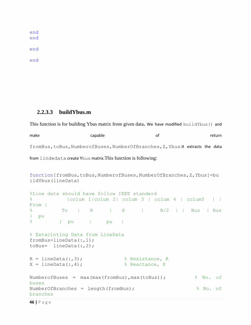
2.2.3.3 buildYbus.m

This function is for building Ybus matrix from given data. We have modified buildYbus() and

make capable of return

fromBus,toBus,NumberofBuses,NumberOfBranches,Z,Ybus.It extracts the data

from lindedata create Ybus matrix.This function is following:

function[fromBus,toBus,NumberofBuses,NumberOfBranches,Z,Ybus]=bu

ildYbus(lineData)

%Line data should have follow IEEE standerd % |colum 1|colum 2| colum 3 | colum 4 | colum5 | |

From | % To | R | X | B/2 | | Bus | Bus

| pu % | pu | pu |

% Extacinting Data from LineData fromBus=lineData(:,1); toBus= lineData(:,2);

R = lineData(:,3); % Resistance, R X = lineData(:,4); % Reactance, X

NumberofBuses = max(max(fromBus),max(toBus)); % No. of

buses NumberOfBranches = length(fromBus); % No. of

branches

47 | P a g e

Z= R + 1i*X; % z matrix yba= ones(NumberOfBranches,1)./Z; % branch

admittance

%innisialYbus

Ybus=zeros(NumberofBuses,NumberofBuses);

%Bulding off-Diagonal Elements of Y-Bus for m=1:NumberOfBranches; iffromBus(m)>0 &&toBus(m)>0 Ybus(fromBus(m),toBus(m))=-yba(m); Ybus(toBus(m),fromBus(m))= Ybus(fromBus(m),toBus(m)); end end

% Bulding of the diagonal elements of Y-Bus

for m=1:NumberofBuses; for n=1:NumberOfBranches iffromBus(n)==m|| toBus(n)==m Ybus(m,m)=Ybus(m,m)+yba(n); end end

2.2.3.4 complexRuseltValue

This simple function is just for result representation purpose .It helps to create matlab output

format on console. The function is following

function[] = complexRuseltValue(frbus,toBus,real,img)

%formating Table like output

48 | P a g e

fprintf(' %5g', frbus) fprintf(' %5g', toBus) fprintf(' %11.4g', real) fprintf(' %12.4g\n', img) end

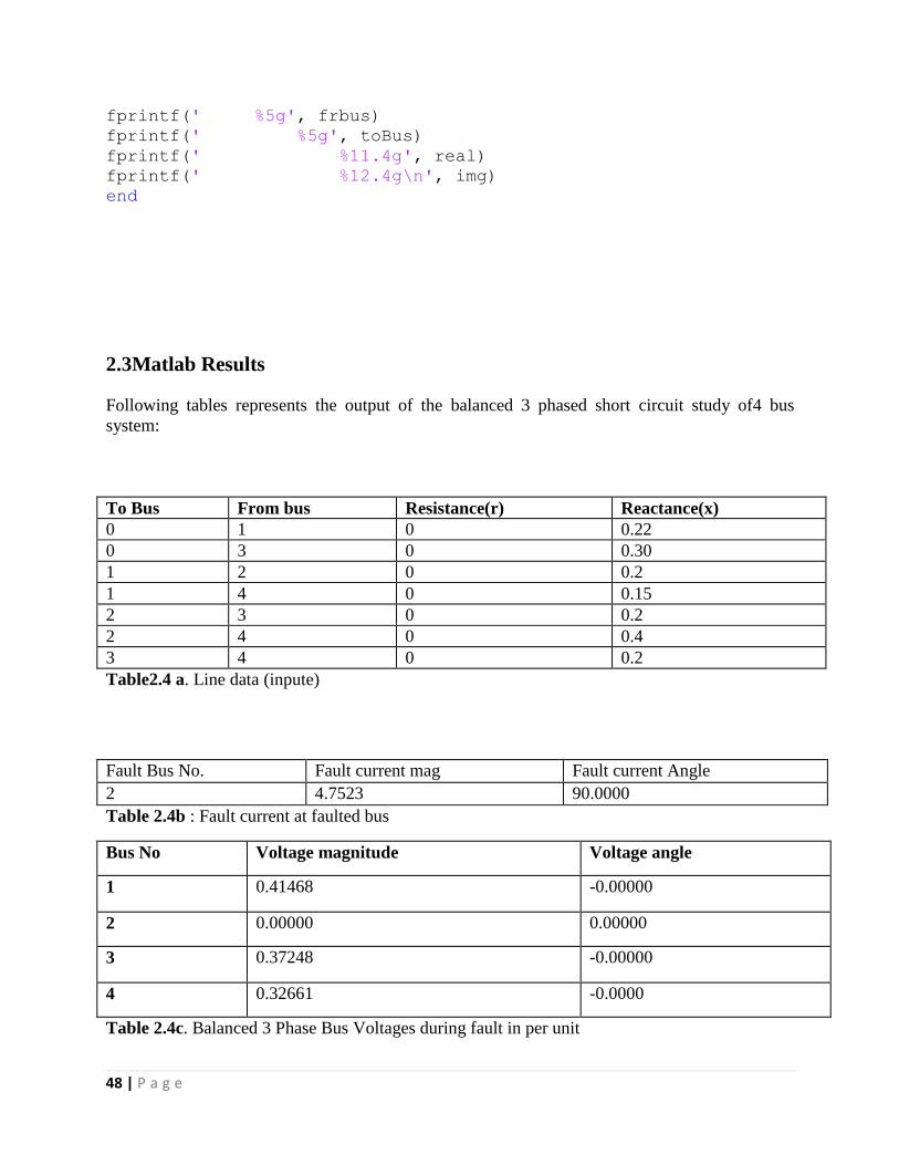
2.3Matlab Results Following tables represents the output of the balanced 3 phased short circuit study of4 bus

system:

To Bus From bus Resistance(r) Reactance(x)

0 1 0 0.22

0 3 0 0.30

1 2 0 0.2

1 4 0 0.15

2 3 0 0.2

2 4 0 0.4

3 4 0 0.2

Table2.4 a. Line data (inpute)

Fault Bus No. Fault current mag Fault current Angle

2 4.7523 90.0000

Table 2.4b : Fault current at faulted bus

Bus No Voltage magnitude Voltage angle

1 0.41468 -0.00000

2 0.00000 0.00000

3 0.37248 -0.00000

4 0.32661 -0.0000

Table 2.4c. Balanced 3 Phase Bus Voltages during fault in per unit

49 | P a g e

From Bus To Bus Current magnitude Current Angle

1 2 2.0734 90.0000

1 4 0.5872 90.0000

2 2 1.8624 -90.0000

2 4 0.8165 -90.0000

3 4 0.2294 90.0000

Table 2.4d . Balanced 3 Phase Bus Voltages during fault in per unit

50 | P a g e

2.4 Flow chart of execution

This Chapter presents the methodology of this project. The methodology is divided into two

parts, which is the simulation and analysis of fault in MATLAB and the development of the

Fault Analysis program using MATLAB GUIDE. The work flow is shown as follows-

51 | P a g e

Chapter - 3

CONCLUSION

3.1 Finale

Figure 2.4 Shows work flow project

52 | P a g e

Various methods for the calculation of short circuit currents have been developed and

subsequently included in standards and in this “MATLAB using p-inverse” publication as well.

A number of these methods were initially designed in such a way that short-circuit currents could

be calculated by hand or using a small calculator. Over the years, the standards have been revised

and the methods have often been modified to provide greater accuracy and a better representation

of reality. However, in the process, they have become more complicated and time-consuming

where hand calculations are possible only for the simplest cases. With the development of ever

more sophisticated computerized calculations, electrical-installation designers have developed

software meeting their particular needs. All computer programs designed to calculate short-

circuit currents are predominantly concerned with:

Determining the required breaking and making capacities of switchgear and the

electromechanical withstand capabilities of equipment

Determining the settings for protection relays and fuse ratings to ensure a high level of

discrimination in the electrical network

Considering above our project will be helpful for calculating the big system with MATLAB

using p-inverse programme. It will be easier for the user to handle and observe the hand

calculation parallel to the MATLAB calculation of a big system's short circuit calculation.

3.2 Shortcoming

In this project we are trying to solve the calculation of the short circuit fault current using

MATLAB with the help of a pre designed function named ,p-inverse. We havetried our best to

finish our project. Our project is worked in small bus system very efficiently. But while

53 | P a g e

performing in the big bus system there is some partial error which is considered as very few

error. This error can be solved in future and higher optimization project.

3.3 Scopes of Project

The scope of the project is to build a package to assist user to perform the fault analysis

calculations with less errors. The targeted user is among trainee engineer and power system

students which have less experience in computer programming or C language. In order to

achieve the objectives of the project, some command in MATLAB program should be studied

and understand so that the package would operate as desired.

Reference

1. http://www.lightning.ece.ufl.edu/PDF/01516222.pdf

2. Grainger, John J. (2003). Power System Analysis. Tata McGraw-Hill. p. 380. ISBN 978-

0-07-058515-7.

54 | P a g e

3. "INVESTIGATING TREE-CAUSED FAULTS | Reliability & Safety content from

TDWorld"

4. Murari Mohan Saha, Jan Izykowski, Eugeniusz Rosolowski Fault Location on Power

Networks Springer, 2009 ISBN 1-84882-885-3, page 339

5. Smth,Paul, Furse, Cynthia and Gunther, Jacob. "Analysis of Spread Spectrum Time

Domain Reflectometry for Wire Fault Location." IEEE Sensors Journal. December, 2005.

6. Edward J. Tyler, 2005 National Electrical Estimator , Craftsman Book Company, 2004

ISBN 1-57218-143-5 page 90

7. Westinghouse Electric Corporation Electrical Transmission and Distribution Reference

Book Fourth Edition, East Pittsburg, Pennsylvania 1959 chapters 1-7, 14

8. J.C. Das, “Calculations of generator source short-circuit current according to ANSI/IEEE

and IEC standards, with EMTP verifications”, Proc. Pulp and Paper Industry Technical

Conference, June 21-26, 2009, pp. 205-215.

9. Electrical Installation Guide In English in accordance with IEC 60364: 2005 edition.In

French in accordance with NF C15-100: 2004 edition.Published by Schneider Electric

(Schneider Training Institute).

10. Analysis of three-phase networks in disturbed operating conditions using symmetrical

components, Cahier Technique no. 18 - B. DE METZ-NOBLAT

11. 1AD Graham, ET Schonholzer. Line Harmonics of Converters with DC-Motor Loads.

IEEE Trans IndAppl 19: 84-93, 1983.

12. JC Read. The Calculation of Rectifier and Inverter Performance Characteristics. JIEE,

UK, 495-509, 1945.

13. MGr„tzbach, R Redmann. Line Current Harmonics of VSI-Fed Adjustable-Speed Drives.

IEEE Trans IndAppl 36: 683-690, 2000.

55 | P a g e

short circuit study of a balanced 3 phase system using p

Documents