Shirking, Sorting, and Reelection in Congress

Bruce Bender Timothy C. Haas Sunwoong Kim

University of Wisconsin-Milwaukee

March 9, 2004

Abstract In the literature on shirking with respect to constituent interests by legislators, the attempts to identify shirking have relied on the proxy of voting score indexes and have been shown to suffer from conceptual or econometric problems. None of these attempts actually estimated the degree of shirking. The objective of this paper is to estimate shirking by members of the U.S. House of Representatives. We accomplish this by developing a stochastic dynamic model of the incumbent's optimization problem while also allowing for a self-selected population of challengers and turnover of congressional seats. The parameter values of the model are numerically estimated using the method of minimum chi-squared. Estimated parameter values are consistent with voters' disciplining shirking incumbents at the ballot box and with challengers self-selecting on the basis of the degree to which their interests and the voters’ interests coincide. Simulations based on the estimated parameter values indicate that the voters’ punishment of shirking congressmen induces incumbents to shirk little in absolute terms and considerably less than if unconstrained by the voters. Furthermore, estimates of mean shirking by terms-served categories are consistent with the empirical findings of no significant last-period problem with respect to shirking.

Shirking, Sorting, and Reelection in Congress* 1. INTRODUCTION There is a large literature on shirking by congressmen, where shirking is the failure of the

congressman to faithfully serve the interests of his constituents.1 Unfortunately, shirking by congressmen

is not directly measurable. The literature has focused, however, on two ways to identify the existence of

shirking. The first approach has been to determine the degree to which the congressman’s personal

ideology influences his voting on legislation to the detriment of his constituents’ interests. This approach

reached its pinnacle with the innovative two-stage methodologies of Carson and Oppenheimer (1984) and

Kalt and Zupan (1984) that spawned over the succeeding years an enormous number of articles

implementing this methodology. Conceptual problems (Lott and Davis [1992], Goff and Grier [1993],

and Bender [1994]) and econometric problems (Jackson and Kingdon [1992]) eventually led to its

abandonment. The second approach has been an examination of the last-period problem in politics. This

approach has been concerned more with the voters’ ability to sort out of office shirking politicians than

with an actual measurement of shirking. Specifically, if voters can successfully perform this sorting

function early enough in a shirking politician’s career, then those surviving politicians will be the ones

whose interests coincide with their constituents’ interests and therefore the ones who will have no

incentive to shirk in their last term in office when the reelection constraint no longer exists. While the

evidence of no significant change in voting records for congressmen in their last terms indicates no

significant last-period problem (Lott [1987; 1990], Van Beek [1991], and Lott and Bronars [1993]), this

approach does not explicitly measure the degree of shirking in the last term and certainly not in preceding

terms in office.

While the literature recognizes the linkage between shirking and the likelihood of reelection, the

lack of a quantifiable estimate of the degree of shirking is a direct result of the lack of a model of the

*The authors benefited from comments on earlier drafts by George Tolley, Roy Gilbert, Ed Lopez, John Patty, Sol Shalit, and seminar participants at the University of Chicago. The authors thank Michael Kim for helping with the data collection.

2

reelection process that lends itself to the estimation of shirking. The objectives of this paper are to

develop and estimate a stochastic dynamic model of the reelection process that includes optimal behavior

in office by incumbents, a self-selected (in the sense of the degree to which the interests of the challengers

and their potential constituents coincide) population of challengers, and turnover of the congress so that

the degree of shirking can be directly calculated from the estimated parameter values. By taking into

account both optimal shirking by incumbents and self-selection by challengers shirking is the outcome of

both moral hazard and adverse selection problems. Furthermore, the estimation of shirking is done

without resorting to the use of an empirical proxy for shirking despite the fact that the degree of shirking

is not directly measurable. The model does, however, abstract from considerations of party and the

seniority system as independent influences on a congressman's behavior in office in order to focus on the

relationship between constituent and congressman.2

Our treatment of the incumbent’s constrained maximization problem is similar in approach to

Lott and Reed’s (1989).3 The utility per congressional term received by the incumbent is assumed to

depend upon the degree to which the incumbent acts in office to serve his own interests. The probability

that the incumbent continues in office is a direct function of the degree to which the incumbent serves the

interests of his constituents. Accordingly the incumbent’s optimal time path of shirking is determined by

a constrained dynamic maximization of expected discounted utility. Furthermore, a self-selected

population of challengers stands ready to replace the incumbent should he leave office. Aggregation of

the results of the constrained choices of the individual incumbents determines the behavior and tenure

structure of the congress over time.

The model is quite parsimonious, consisting of a relatively small number of behavioral equations

and requiring a relatively small number of parameters to be estimated. Each parameter has an explicit and

1See Bender and Lott (1996) for a critical overview of the shirking literature. 2 We do not imply that the impact of party and the seniority system on a congressman's behavior in office is necessarily trivial. We do feel, however, that constituency preference is the primary influence on such behavior and leave the introduction of party and seniority to future work. 3 Unlike Lott and Reed, however, we explicitly solve, albeit numerically rather than analytically, the incumbent’s problem.

3

precise interpretation regarding the voters’ sorting function or the self-selection of challengers. The actual

estimation of parameter values is not accomplished by typical regression techniques. Instead, the

parameter values of the model are numerically estimated by the method of minimum chi-squared first

suggested by Neyman (1949).

Specifically, we simulate the retirement of incumbents and then the dynamic optimal choices of

the incumbents who run for reelection for a given set of parameter values for thirteen successive

congresses. Congressmen who retire or who are defeated are replaced by challengers from a population

whose distribution of preferences is characterized by a set of parameter values. We then compare the

terms served of defeated simulated congressmen over the thirteen congresses with the terms served of

defeated actual congressmen over the thirteen congresses from 1974 to 1998. Parameter values are then

perturbed and the process repeated until there is convergence to a set of parameter values that maximizes

goodness of fit as measured by Pearson’s chi-squared statistic. Given these estimated parameter values,

we can then simulate incumbent shirking.

The null hypothesis that the simulated and actual numbers of defeated congressmen by terms-

served categories are generated by the same process cannot be statistically rejected. Estimated parameter

values are consistent with voters punishing at the ballot box congressmen who shirk and with

congressional challengers self-selecting so that those challengers with a lower propensity to shirk are

more likely to run for office. Note that such self-selection can rationally occur only if voters can sort

incumbents according to their degree of faithfulness to the voters’ interests. Sorting therefore not only

directly mitigates the moral hazard problem of shirking by incumbent congressmen but also indirectly

mitigates the adverse selection problem.

The calculated mean level of shirking based on the estimated parameter values is quite low in

absolute terms and considerably lower than the mean level of shirking that would exist if congressmen’s

behavior were unconstrained by the voters. Furthermore, even though an individual congressman’s

optimal shirking increases with terms served, the mean level of shirking over all congressmen at first is

fairly constant as the number of terms served increases and then decreases as the number of terms served

4

increases. This is consistent with voters constraining the shirking of incumbent congressmen and over

time sorting out of office those congressmen who are inclined to shirk so that the congressmen with

greater tenure are the ones inclined not to shirk. It also explains why researchers have found no significant

last-period shirking problem.

The next section develops the dynamic model of incumbent behavior. Section 3 considers the

impact of sorting by the voters on self-selection by potential candidates and on the mean level of shirking

for the congress. Section 4 provides a model of shirking and turnover in the congress over time. Section 5

describes the methodology for the estimation of the model’s parameter values, and section 6 presents and

interprets these estimated values. Section 7 simulates and analyzes congressional shirking over time based

on the estimated parameter values. Finally, section 8 presents conclusions.

2. MODEL OF INDIVIDUAL INCUMBENT SHIRKING AND TENURE

Consider a congressman as an agent elected by his constituents to serve their interests. Who is the

principal that the congressman represents? We certainly do not imply that it is the median voter.4 It is

more reasonable to view the faithful congressman as serving Fenno's (1978) reelection constituency or

taking Peltzman's (1984) electoral support-maximizing position. For our purposes we can assume the

existence of a set of positions that the faithful congressman will support and refer to this as the set of

positions desired by the constituent-principal.

We also recognize that a congressman may receive utility from taking other positions not

consistent with the interests of his constituents. Taking such positions may be the result of the

congressman's ideology or interests not being consistent with the interests of his constituents, direct

bribes, bribes in the form of promises of future employment, or any other inducement. This is not to say

that the faithful congressman is morally superior. While he may take the positions desired by his

constituents because he truly receives utility from serving their interests, he may also desire to take those

5

positions because they are consistent with his ideology and interests. The latter is probably closer to

reality. Nevertheless, in either case we will refer to such a congressman as one with a “preference” for

serving the interests of his constituents.

Define a continuous variable, η∈(0,1), as a preference parameter indexing the congressman’s

utility from serving constituent interests. η=0 indicates that the congressman’s preference is strongest for

serving his constituents’ interests, whereas η=1 indicates that it is weakest.5 The congressman’s value of

η is not directly observable by his constituents.

Define a continuous variable, x∈(0,1), that indexes a congressman’s behavior according to the

degree to which the congressman faithfully serves the interests of his constituents. A congressman who

behaves as a perfectly faithful agent for his constituents is characterized as choosing a value of x=0,

whereas a congressman who behaves as a completely unfaithful agent is characterized as choosing a value

of x=1.6 Equivalently, x=0 indicates zero shirking with respect to constituent interests, and x=1 indicates

maximum shirking. The continuous nature of x allows for the existence of a continuum of congressmen

with the degree of shirking increasing as x increases.7 The variable x is clearly a choice variable for the

congressman. A congressman might prefer to choose a value of x greater than zero because such a value

would maximize his utility given his value of η.

The choice of a specific utility function for congressmen should have two properties. First, given

the definitions of η and x, the weaker the congressman’s preference for serving constituents’ interests, the

more the congressman will shirk in order to obtain his unconstrained maximum possible utility (i.e., in the

absence of the reelection constraint). Second, for the purpose of avoiding the introduction of bias into the

4 For critiques of the median voter model of elections see, for example, Stigler (1972), Fiorina (1974), Peltzman (1984), Romer and Rosenthal (1984), Goff and Grier (1993), Bender (1994), and Jung, Kenny, and Lott (1994). Bender and Lott (1996) provide an overview of the literature. 5 Although η is defined on the open interval (0,1), we refer to η taking the benchmark values of 0 and 1 for expositional purposes. 6 As in the case of η, we refer to x taking the benchmark values of 0 and 1 for expositional purposes even though x is defined on the open interval (0,1). 7 Our characterization of behavior by the variable x is in the spirit of Sutter's (1998) characterization of congressmen as “angels” and “knaves” except that we allow for a continuum of behavior.

6

model, the unconstrained maximum utility should be the same for each congressman. This standardizes

the potential payoff or maximum possible utility across congressmen.

Let the utility received by a congressman serving term t in office, ut(x(t)), be defined as

(1) ut(x(t)) = η1η

η1η

)η1(η))t(x1()t(x−

−

−−

.

This utility function has both of the desired properties above. The unconstrained maximum utility for a

congressman is obtained when the congressman serves with a degree of shirking of x(t)=η. The

unconstrained maximum utility for each congressman is equal to one regardless of his value of η.8

We assume that each incumbent who runs for reelection receives greater expected utility from

holding office than from being a private citizen. We also assume that each incumbent has a planning

horizon or maximum number of possible terms in office over which he chooses his optimal dynamic

behavior. Although the length of the planning horizon may vary across congressmen for purely

idiosyncratic reasons, there is no way of discerning those reasons. We therefore treat all congressmen

identically by constructing the planning horizon for each congressman using an assumed mandatory

retirement age of R. If we denote Ac as the age at which the incumbent was first elected (i.e., the age at

which he became a successful challenger, hence the subscript c), then the planning horizon or maximum

number of two-year terms that the congressman can serve is denoted as T=(R-Ac)/2.9 The assumption that

each congressman running for reelection receives greater expected utility as a congressman than as a

private citizen coupled with the assumed mandatory retirement age implies that T is indeed a planning

horizon. If the congressman has already served m terms, then the planning horizon shrinks to T-m terms.

8 Note that η has been defined to take values only in the open interval (0,1) because the right-hand side of equation (1) is undefined for the benchmark values of 0 and 1 used for expositional purposes. Further note that the benchmark values of 0 and 1 for x imply that ut(x(t))=0, which is why x also takes values only in (0,1). 9 If (R-Ac)/2 is not an integer, then its value will be rounded up to the next integer.

7

The value of T is congressman-specific. Finally, we assume that voters vote retrospectively.10

Setting a maximum of T terms for an incumbent does not necessarily mean that the incumbent

will serve T terms. Defeat at the polls is possible. Even if the incumbent could be continuously reelected

for the T terms, death and morbidity are stochastic, and, to at least some degree, are other reasons for

leaving office such as retirement in the sense of leaving the labor force, the opportunity to take a cabinet

position or judgeship, and the opportunity to run for governor or senator.

With respect to the incumbent’s bid for reelection, we presume that the challenger cannot win the

election but that the incumbent can lose the election. This is not a play on words. If the incumbent has

served the interests of his constituents while in office, then his campaign promises to do so will have

more credibility than the challenger's precisely because the incumbent has established such a record in

office.11 If the incumbent has served less well, then his credibility and consequently his reelection

probability will be reduced. Although other factors may affect a voter's decision whether to vote for the

incumbent, we model that decision as a function of how well the incumbent has served the interests of his

constituents in his most recent term.

Our specific probability of reelection function (i.e., voters’ sorting function) is

(2) Pt+1(x(t)) = α exp(-λx(t)).

where Pt+1(x(t)) is the probability that the incumbent congressman is reelected for term t+1, x(t) is the

10 There is considerable evidence that voters appear to use a retrospective voting strategy in voting for incumbents. See Francis, Kenny, Morton, and Schmidt (1994). 11 Bernhardt and Ingberman (1985) and Ingberman (1989) treat risk-averse voters as viewing a campaign promise as the expected value of the position that will be taken by the candidate if elected but as viewing the variance around that expected value as smaller for the incumbent if the incumbent's promise is consistent with the past position taken by the incumbent in office. Dougan and Munger (1989) treat the incumbent's reputation for ideological commitment to positions the voters agree with as serving the function in political markets that brand name serves in economic markets. The η value of the challenger, even a potentially faithful challenger with an η value of zero, and the η value of the incumbent are not directly observable by the voters. Only if the behavior of the incumbent were unconstrained (i.e., if there were no future reelection campaign) would the incumbent's η value be directly observable. However, voters have direct observations of the incumbent's behavior in office, x(t), but no such direct observations of the challenger's.

8

degree to which the congressman shirked with respect to the interests of his constituents in term t, the

parameter α is the probability that a perfectly faithful incumbent (i.e., x(t)=0) is reelected,12 and the

parameter λ>0 indicates the reduction of reelection probability caused by the degree to which the

incumbent shirked. Note that the probability of reelection function is a negative exponential function13

and α is the vertical axis intercept of that function. As an illustration of equation (2), if α=0.9, λ=2, and

x(t)=0.1, then the congressman’s probability of continuing for term t+1 is 0.74.

If the incumbent were to lose the reelection bid, then he obviously would be replaced in office by

the victorious challenger. We treat the challenger as being randomly drawn from a population of potential

challengers characterized by a joint distribution of η and Ac that will be specified later.

The objective of an incumbent serving term m in office is to maximize the expected utility

received over a career of T-m+1 potential terms in office given the reelection constraint. The incumbent

does so by his behavior in office over time or his choices of the values of x(t), t=m,m+1,…,T. Note that

even though there is a maximum of T-m+1 remaining terms in office, the voters’ sorting function (2)

makes the actual number of terms that will be served stochastic.

Each incumbent running for reelection must receive greater expected utility from holding office

than from being a private citizen. Otherwise the incumbent would not run for reelection. Denote the

utility per time period of a private citizen as H, where 0≤H<1. Foregone utility per time period as a

private citizen is the opportunity cost of being a congressman and therefore is the utility that a

congressman will receive if he fails to be reelected. The larger is that opportunity cost, the less faithfully

will the congressman serve his constituents ceteris paribus.

Unfortunately, H is not observable. Even if we had data on the wage rates of congressmen prior

to obtaining office, this would not be equivalent to their utilities as private citizens. It is not all that

12 It is not necessary that α be equal to one, although clearly 0≤α≤1. If voters perceive x(t)=0 with some noise, then α will be less than one. The precise value of α is an empirical matter. 13 Even though (2) relates the probability of the incumbent's winning reelection for term t+1 to the degree of shirking by the incumbent during term t, it is not a probability density function and there is no reason that it should be.

9

uncommon for people to take pay cuts when becoming congressmen. Furthermore, the relevant

opportunity cost, H, is not the utility received prior to becoming a congressman but the utility that would

be received as a private citizen after leaving office. This is even more problematic because the

opportunity set facing a congressman after leaving office is certain to be larger than the opportunity set

before taking office.

We therefore assume that the opportunity cost of the utility that would be received as a private

citizen is the same for all incumbents and, more specifically, set that opportunity cost equal to zero. This

assumption is less damaging to the extent that there is no reason to believe that congressmen’s

preferences (η values) are systematically related to their opportunity costs. However, even if the

correlation of preference and opportunity cost were zero for the population of congressmen, this would

not imply that all congressmen must have the same opportunity cost. Our assuming away these

idiosyncratic differences in opportunity cost, thereby ignoring H in the congressman’s dynamic

optimization problem, will have the likely effect of reducing the ability of the model to fit the data.

Denote the maximum lifetime expected discounted utility of an incumbent in term t (for the

period between t and T) as Ue(t) and the comparable utility for a private citizen as Up(t).14 In the last time

period (t=T) the incumbent will have an unconstrained maximization problem because there are no more

future elections (i.e., the probability of continuing for another term, PT+1, is zero regardless of the value of

x(T) that the incumbent chooses). That is, he will choose x*(T) in order to maximize the utility function

defined in (1), where x* denotes the value of x that maximizes utility. His solution is x*(T) = η, and his

utility for the period is one. For a non-terminal period (1≤t<T), the lifetime utilities are recursively

determined by choosing the values of x*(t), x*(t+1), x*(t+2), …, x*(T-1), and x*(T) that satisfy

(3) Ue(t) = max{x(t)} [ut(x(t)) + δ{Pt+1(x(t))Ue(t+1) + (1-Pt+1(x(t)))Up(t+1)}],

10

where δ = (1+r)-2 is the real discount factor for one term (two years) and r is the real one-year opportunity

cost.

The process of solving for the values of x*(t) or the values of optimal shirking over time can be

performed recursively backwards from T to the first period. For example, consider the next to the last

period (t=T-1). The incumbent will choose x*(T-1) to maximize expected utility for the periods T-1 and

T. His choice of x*(T-1) determines his utility in T-1 and probability of reelection for period T by

equation (2). If reelected, he will receive Ue(T)=1 in period T by choosing x*(T)=η in period T. If not

reelected, then he will receive Up(T)=H as a private citizen. As previously noted, when solving (3) for the

x*(t) values we set H=0. Similarly, the incumbent in period t=T-2 chooses the optimal x*(T-2). For any

given pair of values of the parameters, α and λ, and any given value of the incumbent's preference

parameter, η, the incumbent's optimal degree of shirking, x*(t), will increase monotonically as t increases

until x*(T) = η, the incumbent's unconstrained degree of shirking, in the final period of the incumbent's

time horizon. Finally, note that even though T, the maximum number of terms that the incumbent can

serve, is exogenous to the model, the actual number of terms served is endogenous because it is

dependent upon the incumbent's sequential choice of the x(t) values. Equation (3) can be solved for the

optimal values of x(t) by numerical methods.15

3. IMPACT OF SORTING ON SELF-SELECTION AND THE MEAN LEVEL OF SHIRKING

For any degree of electoral discipline imposed by the voters (i.e., the specific values of α and λ in

the voters' sorting function (2)), optimizing behavior by the individual incumbent will result in

congressmen with higher values of the shirking preference parameter, η, having higher time paths of

14 The subscripts e and p refer to the incumbent (e for elected congressman) and the private citizen (p for private citizen). 15 It is interesting to contrast our optimization problem by the candidate to those in the “citizen-candidate models” by Osborne and Slivinski (1996) and Besley and Coate (1997). In their one-term models the candidate implements his policy preference if elected, just like the incumbent in our model in the last term of his time horizon. The key decision variable in their models is whether to run for office based on maximizing expected utility given the candidate’s policy preference. In our dynamic model, the key decision variable is how much the incumbent will

11

optimal shirking than congressmen with lower values of η. It follows that congressmen with higher values

of η will have a smaller expected number of terms served than will congressmen with lower values of η.

Consequently, sorting by the voters not only constrains incumbents' shirking in the earlier terms of their

careers but also reduces shirking by more quickly removing from office those incumbents with greater

preference to shirk.

There also is an indirect way in which sorting affects the overall level of shirking. Sorting by the

voters implies that a successful challenger with a lower η value can expect a greater number of terms in

office and a larger utility in each term than would a successful challenger with a higher η value. Since

running for office, especially the first time, is not costless, we can treat this cost as equivalent to an entry

fee or initial outlay for an investment. A challenger with a lower η value therefore can expect a higher

return on investment than a challenger with a higher η value16 and therefore would be more likely to run

for office. Consequently, the distribution of η for the population of challengers therefore should be one

for which smaller values of η are more likely to be observed than are larger values of η. This self-

selection toward challengers with a smaller preference for shirking is a result of sorting by the voters.17

Electoral discipline imposed by the voters not only reduces shirking by incumbents but also induces

challengers to self-select in terms of preference for shirking.

Choosing a specific distribution of η consistent with the above reasoning still has some degree of

arbitrariness because η is not directly observable. We greatly reduce this arbitrariness factor by selecting

a family of distributions. We let the distribution of η for challengers be a beta distribution described

below:

shirk (i.e., will deviate from the constituency’s preference) over time so as to maximize the expected present value of utility over a sequence of potential terms in office given the incumbent’s preferences. 16 Indeed, if the initial outlay is sufficiently large, then there is no guarantee that the rate of return on investment will even be positive for a challenger with a high η value. 17 To see this starkly, suppose that sorting of incumbents did not occur – i.e., incumbents continued in office according to a random process. This would imply that all incumbents would have the same expected tenure in office and all would receive the same utility each term because each would choose x(t)=η regardless of their η values. There would be no incentive for self-selection by challengers. In this case the best guess for the distribution of η for the population of challengers would be a uniform distribution.

12

(4) f(η) = B(a,b)-1ηa-1(1-η)b-1 0≤η≤1

= 0 otherwise,

where a and b are parameters with a>0 and b>0 and B(a,b) = 0∫1 ηa-1(1-η)b-1 dη. This distribution is

defined on (0,1), as is η, and is quite flexible. The expected value is a/(a+b), a=1=b yields a uniform

distribution, a>1 and b>1 yields a unimodal distribution, and a value of (a/b) that is <1 (>1) yields a

distribution skewed to the left (right). A sufficiently small value of (a/b) will produce a distribution that is

close to one that is monotonically decreasing.

Since our objective is to estimate the overall level of shirking in the U. S. House of

Representatives over time, we need to specify an initial congress. This initial congress is simply a sitting

congress that is designated as the initial congress in our series of congresses. We expect that the

distribution of η for the incumbents in this initial congress is one for which smaller values of η are more

likely to be observed than are larger values of η because congressmen with low η values are likely to

have survived longer in office than the congressmen with the high η values given sorting by the voters.

As was the case when looking at the population of challengers, we let the distribution of η for the

congressmen in this initial congress be described by the beta distribution below:

(5) g(η) = B(c,d)-1ηc-1(1-η)d-1 0≤η≤1

= 0 otherwise.

Estimation of the values of the parameters, α and λ, of the voters' sorting function in equation (2),

the values of the parameters, a and b, of the distribution of η for the challengers population in equation

(4), and the values of the parameters, c and d, of the distribution of η for the congressmen in the initial

congress in equation (5) is necessary to allow the estimation of the mean level of shirking in the congress

13

over time. The next section develops an aggregated model of shirking and turnover for the congress over

time that is amenable to the estimation of the parameter values. The succeeding section describes the

estimation procedure.

4. MODEL OF SHIRKING AND TURNOVER IN THE CONGRESS OVER TIME

We start with an initial congress with each incumbent congressman characterized by number of

terms served, preference for shirking or η value, and age. Given the incumbent's utility function in

equation (1) and the voters' sorting function with its parameters, α and λ, in equation (2), the incumbent

dynamically maximizes expected discounted utility over the terms remaining until the mandatory

retirement at age R by choosing the optimal time path of shirking over those terms according to equation

(3). Shirking in any term t determines the probability that the incumbent is reelected to term t+1. Should

the incumbent be defeated for reelection to another term, then the incumbent is replaced in office by a

challenger with a specific age and η value. While the incumbent in our model is automatically retired at

age R, it is possible for the incumbent to retire before age R for stochastic reasons. A retired incumbent is

replaced by a challenger with a specific age and η value. The next congress is composed of those

incumbents who were reelected and the challengers who replaced either defeated or retired incumbents.

Each incumbent in this new congress is characterized by number of terms served, η value, and age. Each

incumbent optimally shirks in the new term, and defeated or retired incumbents are replaced by a new set

of challengers in the succeeding congress. Over time we construct a series of congresses consisting of

incumbents with specific values of terms served, η, and age who optimally shirk in each congress. We

can then address questions such as the mean level of shirking in congress, the relationship between

shirking and terms served, and the last-period shirking problem.

At this stage, however, equations (1), (2), and (3) can only determine the probability of reelection

of an incumbent with a specific number of terms served, η value, and age. Whether the incumbent is

actually reelected or defeated must be determined stochastically in light of the reelection probability.

14

While equation (4) specifies a marginal distribution of η for the challenger population, the actual η value

and age of the challenger succeeding a defeated or retired incumbent must be stochastically determined in

light of a joint probability distribution of η and age. While equation (5) specifies a marginal distribution

of η for the incumbents in the initial congress, the actual number of terms served, η values, and ages of

the incumbents in the initial congress must be stochastically determined in light of a joint probability

distribution of terms served, η, and age. Furthermore, in order for the model to generate quantitative

results it is necessary to estimate the parameter values, α and λ, of the voters' sorting function in (2), the

parameter values, a and b, of the marginal distribution of η for challengers in (4), and the parameter

values, c and d, of the marginal distribution of η for the sitting incumbents in the initial congress in (5).

The next section constructs the joint probability distributions in the course of describing the methodology

for estimating the values of the parameters.

5. METHODOLOGY FOR ESTIMATING PARAMETER VALUES

5.1. Overview of the estimation methodology

We start with an initial congress of 435 congressmen because there are 435 members of the U. S.

House of Representatives. Given an initial set of parameter values we simulate the optimal shirking of the

incumbents over a series of thirteen successive congresses. After each congress defeated and retired

incumbents are replaced by successors randomly drawn from the population of challengers. We then

perturb the parameter values and rerun the simulations of the thirteen successive congresses. The

parameter values are perturbed and the simulations rerun until we have observations of the outcomes of

the optimal behavior of the incumbents in the simulated congresses which, when compared to the

observations of the outcomes of the behavior of the incumbents in the actual congresses, minimizes the

value of the chi-squared statistic. The obvious first question is what outcome of incumbent behavior to

choose.

Our choice is the number of terms that an incumbent serves until he is defeated for reelection. It

15

is not unreasonable to ask a model of electoral behavior to make this prediction. We therefore create the

categories labeled “ts terms served at the time of electoral defeat,” where ts=1,2,3,…,21, and compare the

number of actual and expected incumbents in each category.18 Note that since each observation is an

individual incumbent who, by the nature of the categories, can only be counted once, the chi-squared

distribution’s assumption of the independence of observations is not violated.19 The data for terms served

at the time of defeat in each electoral category is compiled for the thirteen congresses from 1974 through

1998 that comprise our sample.20

Pearson's chi-squared statistic is

(6) χ2 = (observed∑=

m

1ii –expectedi)2/(expectedi),

where m is the number of cells or “ts terms served at the time of electoral defeat” categories.21 The

methodology for calculating the expected number of congressmen in each cell will be described in the

next subsection. Note that minimizing the value of the chi-squared statistic is equivalent to minimizing

the normalized sum of the squared deviations of the actual from the expected number of congressmen in

the cells.

18 The last category is “21 terms served at the time of electoral defeat” because this is the largest number of terms that any defeated incumbent in our data set served. 19 The assumption of independence of observations of the chi-squared distribution rules out other seemingly attractive alternative implications of the electoral model. One such alternative is the number of incumbents in each terms-served cohort – i.e., the tenure structure of the congress. This alternative violates the independence of observations assumption because any incumbent who has served n terms must have served n-1 terms in the preceding congress, n-2 terms in the congress before that one, and so on. Only if each observation is a single individual and each individual can only constitute a single observation will the independence of observations assumption be satisfied. 20 The data sources for all our data are the 1976 through 2000 editions of the Almanac of American Politics and the 2000 edition of the Congressional Biographical Directory. 21 Note that by comparing the actual defeated incumbents and the expected defeated incumbents in each of the terms-served categories for the whole thirteen-election period, we are really testing the long-run explanatory ability of our model. The noise associated with the data of defeated incumbents in any single election year makes a

16

5.2. The estimation methodology

This subsection puts the flesh on the bones described in the overview. Specifically, we describe

the following in detail: handling the retirement of congressmen; generating the joint distribution of η and

age for challengers; calculating the expected number of congressmen in each cell of the chi-squared

distribution; generating the joint distribution of terms served, η, and age of the congressmen in the initial

congress; and the numerical methodology used for the parameter value search.

5.2.1. Retirement

We define the term “retirement” quite broadly in that it refers to voluntarily not running for

reelection for any one of several reasons. A congressman may leave office for normal retirement, personal

reasons, death, or morbidity. A second category of reasons includes running for higher office or accepting

a position such as a judgeship or cabinet secretary. A third category is that the congressman loses his seat

because of redistricting. While in a sense this last category may not be purely voluntary, we treat leaving

office because of redistricting as retirement because it does constitute a decision not to run for

reelection.22

Although we can generically conceptualize the calculus of the incumbent’s retirement decision

(Schansberg [1994]), there is no theoretical model of the retirement decision that relates the probability of

retirement to the number of terms served. The different causes of retirement, as we broadly define it,

virtually guarantee this. However, it is necessary that we have a method for retiring simulated incumbents

statistically acceptable explanation of defeated incumbents by terms-served categories on an election-by-election basis virtually impossible. It is the long-run behavior of congressmen, however, that is of interest. 22 During our sample period 45 seats were eliminated because of redistricting. Many other districts were geographically altered – most in a minor manner, some substantially. It is likely that some incumbents chose not to run for reelection as a result of redistricting, but it is possible only to conjecture which incumbents retired for this reason. There were actually 13 incumbents whose seats disappeared because of redistricting but who still ran for reelection in the new congressional district. 12 of the 13 ran in either a primary or general election against another incumbent. The thirteenth incumbent changed his address so that he could avoid running against another incumbent. Instead he ran against (and lost to) a nonincumbent in a newly created district. We treat all thirteen of these incumbents as if they retired. In the case of the first twelve, it is a certainty that one of the two incumbents in each of the reelection contests would have to lose even if both had been perfectly faithful incumbents. In the case of the thirteenth it is difficult to refer to him as an incumbent running for reelection because he intentionally chose to run in a district that he had never before represented.

17

when simulating congresses over time. In each congress we therefore stochastically retire incumbents by

terms-served category by randomly drawing from an empirical distribution of retirement by terms-served

categories.

In each congress there are 435 actual incumbents. Of these 435-k choose to run for reelection and

k choose to retire, where the value of k varies from congress to congress. We retire k members of the

congress of 435 simulated incumbents.23 We calculate from the data the number of incumbents who

retired after exactly ts terms served, ts=1,2,…,27, and the number of incumbents who served at least ts

terms.24 Dividing the first number by the second yields an empirical frequency rate or probability of

retirement by terms-served category denoted as r(ts).25 At the beginning of each congress k simulated

incumbents are retired as follows. Incumbents are randomly drawn without replacement. If the first

incumbent has, for example, 6 terms served, then his probability of retirement is r(6). Given the value of

r(6) a random number generating process will determine whether or not this incumbent is retired.26

Random draws without replacement continue until the required number of k incumbents is retired. If after

drawing all 435 members of the simulated congress less than k incumbents have been retired, then the

random drawing without replacement begins again from the population of remaining incumbents.

We further impose a restriction for each congressman of a maximum career of T=(R-Ac)/2 two-

year terms, where Ac is the age of the incumbent when first elected to office or, equivalently, the

incumbent's age when he became a successful challenger. Any congressman who will exceed this

maximum number of terms by the end of his current term cannot run for reelection. He is automatically

23 Note that all we are doing is guaranteeing that in each congress the number of simulated incumbents running for reelection is equal to the number of actual incumbents running for reelection. 24 Note that with respect to retirement there are 27 categories of terms served rather than only 21 because in the data set the incumbent with the longest tenure retired after 27 terms. 25 Note that it is not necessary that the sum of all the r(ts) equals one. The calculated retirement probabilities are: r(1)=.02403, r(2)=.06093, r(3)=.09371, r(4)=.10671, r(5)=.14400, r(6)=.14558, r(7)=.12286, r(8)=.15534, r(9)=.17749, r(10)=.18644, r(11)=.08511, r(12)=.26549, r(13)=.15116, r(14)=.15942, r(15)=.26786, r(16)=.29730, r(17)=.20690, r(18)=.35000, r(19)=.33333, r(20)=.20000, r(21)=.25000, r(22)=.60000, r(23)=.00000, r(24)=.50000, r(25)=.00000, r(26)=.00000, and r(27)=1.00000. 26 The empirical value of r(6) is .14558. A random number is drawn from 1 to 100,000. If the number drawn is less than or equal to 14,558, then the incumbent is retired; if the number is greater than 14,558, then the incumbent is not retired.

18

retired at the end of the term and is replaced by a new congressman in the next term. This implies that the

simulated planning horizons of congressmen vary across congressmen according to their ages at the time

they first were elected. For calculating T we choose a mandatory retirement age of R=80.27

5.2.2. Joint distribution of preference parameter and age for the challenger population

In order to draw a successor for a retired or defeated congressman we need to specify a joint

distribution of the unobservable preference parameter, η, and the age, Ac, for the population of

challengers. Assuming that the age of the challenger and his preference for serving constituent interests

are not related, the joint distribution of (η,Ac) is therefore obtained by Pr(η,Ac) = Pr(η)Pr(Ac). The

marginal distribution of η is given in (4). The marginal distribution of Ac is an empirical distribution. It is

constructed from data for the entering age of each of the freshmen congressmen from 1974 through 1998.

This marginal distribution has a mean and standard deviation of 43.5 and 8.7, has minimum and

maximum values of 25 and 71, and is skewed to the left. Challengers who replace defeated or retired

incumbents are randomly drawn from the population of challengers described by the joint distribution of

(η,Ac)

5.2.3. Expected number of congressmen with ts terms served at the time of defeat

We first choose initial values of the parameters of the model. The initial congress has 435

27 The number of congressmen in our data set who did not run for reelection (i.e., “retired”) is 621. The mean age and standard deviation are 56.2 and 11.4, and the minimum and maximum are 32 and 89. The use of the term “retirement” is misleading to some extent as is the relatively low mean of 56.2. Some of those “retiring” congressmen did not run for reelection because they ran for higher office while others took cabinet positions or judgeships. Some died or developed health problems. Some were induced to retire prior to 1992 by legislation eliminating a congressman’s right to keep his unused campaign funds as personal funds unless he had served in Congress before 1980 and retired before 1992 (Burnett, Paul, and Wilhite (1997)). Redistricting involuntarily retired 45 congressmen by eliminating their districts, while an unknown number of other congressmen might have chosen not to run because redistricting radically altered their districts. Taking into account the above causes of “retirement” and the at least partially stochastic nature of these causes, it appears that the job of congressman is one that the jobholders often desire to hold to an old age. Of the 621 congressmen who retired, there were 11 congressmen who retired at age 80 or greater. Of the 957 incumbents in our data set 52 were actually elected for the first time between the ages of 60 and 71. It should be kept in mind, however, that the choice of this endpoint is arbitrary. It should also

19

representatives. Each congressman is characterized by a value of η, a value of ts (terms served), and a

value of As, where As=(Ac+2ts) is the age of the sitting congressman. These values of η, ts, and As for

each congressman in the initial congress are randomly drawn from a joint distribution of η, ts, and As

whose construction is described in the next subsection. By the process described earlier k congressmen

are retired leaving 435-k to run for reelection. During the congressional term each congressman chooses

his optimal degree of shirking, x*(t).28 In the light of the values of α and λ, this choice of x*(t) determines

the probability that the congressman will be reelected to serve in the next term. Given this probability, a

random number generating procedure determines whether the congressman will actually serve another

term. If so, then the congressman's number of terms served is augmented by one and his age as a sitting

congressman, As, is augmented by two.29 If not, then the congressman is replaced in office by a successor

randomly drawn from the pool of challengers characterized by the joint distribution of (η,Ac). When

simulated for all congressmen, the values of η, ts, and As are generated for the members of the next

congress. This process continues for a sequence of thirteen consecutive simulated congresses including

the original simulated congress. We compute the number of defeated simulated congressmen in each

terms-served (ts) category over the thirteen elections. The number of defeated simulated incumbents in

any specified ts category as a fraction of the total number of simulated defeated incumbents for all the ts

categories is the estimated probability that a defeated incumbent will have that specified number of terms

served.

Our model, however, is a stochastic, not deterministic, model. The parameter values determine

probabilities of outcomes at every stage of the model, but the actual outcomes are determined by a

random number generating process in conjunction with those probabilities. Therefore, the estimated

be kept in mind that this is an endpoint for the decision-making time horizon of the individual congressman and not the congressman’s actual retirement age, which can only be known ex post. 28 When optimizing according to equation 3 we use a one-year real opportunity cost, r, of .05, which yields a two-year (one term) real discount rate of δ=(1+r)-2=.907. This reflects investment in a congressional career as more risky than investment in Treasury bonds. 29 If the augmented value of As equals or exceeds the mandatory retirement age, R, then the congressman will not run for any more future reelections and will be replaced by a challenger at the next election.

20

probability that a defeated incumbent will have a specified number of terms served based on just one

simulated run of the model is a random draw from a probability distribution of such estimated

probabilities. However, as the number of replications of the simulations of the thirteen congresses for the

set of specific parameter values increases, the mean value of this estimated probability approaches the

true probability for this set of specific parameter values.30 The expected number of defeated incumbents

with this specific value of terms served is the product of the mean estimated probability for this ts

category and the total number of actual defeated incumbents for all ts categories.31 Having tabulated the

number of actual defeated incumbents for each terms-served category from our data set for the thirteen

elections from 1974 through 1998 and having calculated the expected number of defeated incumbents for

each category for thirteen elections, we can test the null hypothesis that the actual number and simulated

number of defeated incumbents by terms-served categories or cells are generated by the same process by

calculating the value of the chi-squared statistic according to equation (6).

Although there are defeated incumbents with terms served ranging from 1 to 21, we use 12 terms-

served categories or cells instead of 21. This is because the distribution of actual incumbents defeated by

terms served becomes sparse after the cell for eleven terms served.32 The chi-squared test statistic

becomes unreliable when the distribution is sparse. This problem of a sparse distribution can be handled

by combining cells into aggregated cells (Moore (1977)). We therefore choose cells for 1, 2, 3, …, 11,

and 12 through 21 terms served.

After calculating the value of the chi-squared statistic given our initially chosen parameter values,

we choose new values of the parameters and repeat the process. We continue the process searching the

30 Our criterion for the number of replications was to increase the number of replications until the value of the chi-squared statistic demonstrated stability with respect to additional replications. Stability became evident at fifty replications per set of parameter values. 31 Note that for the chi-squared test statistic the determination of the expected number of defeated incumbents in any specific terms-served category is conditioned on the total number of actual defeated incumbents in the data set. See Moore (1977). Also note that it is necessary to round the expected number of defeated incumbents in each terms-served category to an integer. 32 There are seventy-nine defeated incumbents with one term served. This number declines almost monotonically until there are ten defeated incumbents with eleven terms served. There are only three defeated incumbents with twelve terms served. There are no more than four incumbents in any of the cells for terms served of twelve or more. Two of these cells have values of zero and four have values of one.

21

reasonable parameter space until we have the values of the parameters that minimize the value of the chi-

squared statistic.

5.2.4. Joint distribution of preference parameter, terms served, and age for the initial congress

The assignment of the values of η, ts, and As to the congressmen in the initial congress cannot be

done arbitrarily because any arbitrary assignment necessarily biases the estimated values of the

parameters. For example, if we assign values of the unobserved η that are lower than the actual η values

of the congressmen in the 1974 congress, then our estimated value of λ will likely be biased upwards in

order to obtain simulated reelection rates as close as possible to the actual reelection rates for the thirteen

congresses from 1974 through 1998. More generally, any attempt to construct an initial congress that is as

close as possible to the 1974 congress arbitrarily puts more weight on the 1974 congress than on the 1976

through 1998 congresses in the estimation of the parameter values. It is necessary to construct a joint

distribution of η, ts, and As for the initial congress and assign values of η, ts, and As to the

congressmen in this congress by random draw.

The marginal distribution of η is described in equation (5).33 The age of a sitting congressman is

determined by the age at which he was first elected (i.e., when he first became a successful challenger)

and the number of terms he has served by As = Ac + 2ts, where the marginal distribution of Ac is the

previously discussed empirical distribution. The joint distribution of (ts,η,As) follows directly from the

joint distribution of (ts,η,Ac), which is obtained by Bayes' law -- i.e., Pr(ts,η,Ac) = Pr(ts|η,Ac)Pr(η)Pr(Ac).

We now consider the conditional distribution of ts.

The conditional distribution of ts on η and Ac can be approximated as a limiting distribution as

follows. We randomly draw 435 values of η from the marginal distribution characterized by specific

33 Note that the parameters, c and d, of the marginal distribution described in (5) are estimated jointly with the other parameters, α and λ of the sorting function in (2) and a and b of the marginal distribution described in (4), using all thirteen congresses. Consequently, the initial or 1974 congress is given no more additional weight in the estimation of the joint distribution of ts, η, and As than any of the other twelve congresses.

22

values of c and d in (5). We then pair these η values with 435 values of Ac randomly drawn from the

marginal distribution of challenger ages. We now have 435 congressmen, each characterized by an η

value and an Ac value. Each congressman starts with a ts value of 1 and an As value equal to his Ac+2.

The congressman runs in five hundred consecutive elections34 with the voter’s sorting function

characterized by specific values of α and λ. If the congressman is reelected, his ts value is augmented by

one and his As value is augmented by two for the next election provided that the augmented As value is

less than the mandatory retirement age of R; but if his augmented As value is greater than or equal to R or

if he is not reelected, his ts value is set equal to 1 and his As value is set equal to his Ac+2 for the next

election. For this congressman with his specific η value and Ac value, we can calculate the fractions of the

five hundred times that ts takes the values 1, 2, 3, …, 21 and treat these fractions as the probabilities that ts

equals 1, 2, 3, …, 21. When done for all 435 congressmen, we will have the conditional distribution of ts

on η and Ac.

Given the conditional distribution of ts on η and Ac, the marginal distribution of η for

incumbents, and the marginal distribution of Ac, application of Bayes' law yields the joint distribution of

(ts,η,Ac) for the initially chosen values of parameters α, λ, c, and d. The initial congress is constructed by

randomly drawing 435 3-tuples of ts, η, and Ac from this joint distribution. These 3-tuples are directly

converted into 3-tuples of ts, η, and As by As=Ac+ 2ts.

5.2.5. Numerical methodology for the parameter value search

An initial set of values of the parameters, α, λ, a, b, c, and d, are selected. As described earlier the

terms served, η values, and ages of the congressmen in the initial congress are randomly drawn from the

joint distribution of (ts,η,Ac), where the construction of this joint distribution depends upon the specific

values of the parameters, c and d, of the marginal distribution of η in (5) and upon the specific values of

34 Ideally we would like to run a thousand or even more consecutive elections for estimating the limiting distribution but the demands on computer time would be too great.

23

the parameters, α and λ, of the voters' sorting function in (2). Given these specific values of α and λ this

initial congress goes through thirteen reelection cycles with reelected congressmen having their ts values

augmented by one and retired or defeated congressmen replaced by challengers with ts values equal to 1

and η and Ac values randomly drawn from the joint distribution of (η,Ac) for challengers, where the

precise marginal distribution of η in (4) depends upon the specific values of the parameters, a and b.

Based on fifty replications of the selection of the initial congress and the thirteen successive election

cycles, the value of the chi-squared statistic is calculated for the thirteen congresses.35 The values of the

parameters, α, λ, a, b, c, and d, are then perturbed and the whole process of creating the initial congress,

simulating the thirteen reelection cycles, and calculating the chi-squared statistic is repeated. The process

is stopped when the value of the chi-squared statistic is minimized.36 If the value of this chi-squared

statistic indicates that the null hypothesis that the actual data and the simulated data of electoral defeats by

terms-served categories are generated by the same process cannot be rejected, then the parameter values

that generated this minimum chi-squared value are accepted as the parameter values of the model.

6. ESTIMATED PARAMETER VALUES

Based on the above methodology, the estimated parameter values are: a = 2.0097, b = 5.6512, c =

1.6878, d = 6.3485, α =0.9692, and λ = 0.9217. The value of the chi-squared statistic based on the fifty

replications of the model with these parameter values is 8.207. This is below 9.236, which is the critical

value at the .1 significance level for a chi-squared test with 5 degrees of freedom.37 We cannot reject the

null hypothesis that the data and the simulated data of electoral defeats by terms-served categories are

35 The necessity of replications was explained previously in subsection 5.2.3., and the choice of fifty replications was explained in footnote 30. 36 The optimization algorithm used to search for the parameter values is the alternating variables method. See Fletcher (1987). On those occasions when the search algorithm became stuck in a “flat plain” in the seven-dimensional search space we would discretely change selected parameter values. In making these changes we referred to “diagnostic” output along the lines of Table 1 (presented in the next section). 37 The number of degrees of freedom is equal to the number of cells minus one minus the number of parameters. See Moore (1977). The 5 degrees of freedom is equal to 12-1-6.

24

generated by the same process. Furthermore, the power of the test,38 or the probability of rejecting the null

hypothesis when it is false, is .698.

Table 1 provides a more detailed picture of the ability of the model to fit the data. Columns 2 and

3 of the table present the observed number and expected number of defeated incumbents by terms-served

categories. It becomes quickly apparent that the model does an excellent job of explaining the life spans

in office of congressmen serving 3, 4, 5, …, and 11 terms until electoral defeat. The model has a little

difficulty explaining the thin tail of defeated congressmen with 12 or more terms and a little more

difficulty explaining defeats of congressmen with 1 and 2 terms. Column 3 confirms this by indicating the

contribution to the overall value of the chi-squared statistic from each terms-served category.

The estimated parameter values are consistent with the model. Consider the parameters of the

voters’ sorting function (2). The parameter α is the vertical intercept of the sorting function and indicates

the probability that a perfectly faithful incumbent (x(t)=0) running for reelection is reelected. The

estimated value of α is 0.9692, implying that a perfectly faithful incumbent has almost a 97 percent

chance of being reelected. This suggests, at least in the case of an incumbent who does not shirk at all,

that the voters perceive the incumbent’s performance with relatively little noise. The parameter, λ, which

has an estimated value of 0.9217, reflects the degree to which the voters punish shirking by reducing the

probability of reelection.

In order to give an idea of how the estimated parameters of the model imply the probability of an

incumbent successfully running for reelection, an incumbent who shirks with a degree of unfaithfulness

of x(t)=0.02 would have a probability of reelection of 0.951 according to equation (2). In contrast,

incumbents with x(t) values of 0.20 and 0.50 would have reelection probabilities of 0.806 and 0.611. In

order to give an idea of how the model in general performed, the mean probability of reelection of .939

for the thirteen simulated congresses compares favorably to the mean probability of .918 for the thirteen

congresses comprising our data sample.

38 See Brownlee (1965, pp. 98-99) for a general discussion of the power of a test, and see Agresti (1990, pp. 241-

25

The parameters, a and b, are for the beta distribution of η for the population of challengers and

have estimated values of 2.0097 and 5.6512. These values indicate a unimodal distribution that is skewed

to the left with an expected value of 0.26. Potential challengers whose interests are closer to the interests

of the constituents are more likely to seek office than potential challengers whose interests are not. As

explained in section 4 skewness to the left is consistent with rational self-selection by challengers based

on an expected return to running for office criterion39 in the light of sorting of incumbents by the voters.

Indeed, in the absence of sorting there would be no incentive for challengers to self-select and the best

guess for the distribution of the beta distribution of η for the population of challengers would be a

uniform distribution (i.e., a=1=b).

The parameters, c and d, are for the beta distribution of η for congressmen in the initial

legislature and have estimated values of 1.6878 and 6.3485. This distribution is unimodal and skewed to

the left with an expected value of 0.21. The expected value of η for the congressmen in the initial

legislature is less than the expected value of η for the population of challengers. This is consistent with

sorting by the voters because those challengers with the lower η values who are elected are likely to

survive longer in office than those challengers with higher η values who are elected .40

7. ANALYSIS OF SHIRKING

Our analysis of shirking focuses on three issues. First, to what degree does the voters’ sorting

process or the reelection constraint directly limit incumbent congressmen’s shirking? Second, to what

243) for a discussion of power for the chi-squared test. 39 The consistency of our estimated parameter values with an expected utility criterion for seeking office also lends support to Osborne and Slivinski (1996) and Besley and Coate (1997) to the extent that candidates are policy-motivated as well as office-motivated. 40 While consistent with sorting, the smaller expected value of η for the incumbents in the initial congress has to be interpreted with some care. In the absence of an analytic solution for the composition of the congress in the steady state, there is no way of knowing with certainty whether the initial congress in the data set is representative of the congress in the steady state. The composition of the initial congress may have been the result of an exogenous shock to the electoral system. Indeed, the steady state may not be a specific composition of the congress but instead may consist of oscillations around a particular composition. These caveats notwithstanding, it is still accurate to state that the smaller expected value of η for incumbents in the initial congress than for challengers is consistent with voter sorting.

26

degree does the sorting process indirectly limit shirking by inducing political challengers to self-select on

the basis of their likelihood of shirking if elected? Third, what explains the literature’s finding of no

significant last-period shirking?

We start by using the estimated parameter values to simulate the thirteen congresses. Based on

ten replications of the simulations of the thirteen congresses41 mean values of incumbent preferences (η)

and incumbent shirking (x(t)) are calculated for each congress. Figure 1 presents plots of these mean

values.

The mean value of η starts at about 0.21 in simulated congress 1 and gradually increases to about

0.24 by congress 13. This is expected. The distribution of η for the initial congress has an expected value

of 0.21, while the distribution of η for challengers has an expected value of 0.26. As incumbents leave

office over time because of voter sorting or retirement they are replaced by new congressmen from the

challenger population. Over time the expected value of η from the challenger population will become the

upper bound of the possible mean η values of the incumbent population. This turnover of the congress

will push the mean value of η for the congress towards this upper bound of 0.26. Sorting will cause the

mean value to be less than this upper bound as over time voters sort out of office more quickly those

congressmen who are more inclined to shirk.

The mean value of x(t) is fairly constant at about 0.05. In the absence of the reelection constraint,

a congressman will optimally shirk by an amount equal to η. The mean value of η for the congressmen is

0.24, and the expected value of η for the population of challengers is 0.26. Sorting by the voters not only

limits shirking to a small absolute amount of 0.05 but also limits shirking to about twenty percent of what

its unconstrained level would be.

This is, however, only the direct impact of sorting on shirking. The expected value of η of 0.26 is

itself indirectly determined by voter sorting. In the presence of voter sorting there is a higher return to

41 There were negligible differences in the plots of figure 1 when going from three to four replications. Ten replications are therefore more than sufficient to be confident that any noise in the plots is quite small.

27

holding office for those congressmen with lower values of η. Such congressman will receive more utility

per term served and can expect to serve more terms than congressmen with higher values of η. Self-

selection by challengers on the basis of expected return therefore will cause the distribution of η values

for challengers to be skewed to the left and to have an expected value less than 0.5 as is the case for the

estimated distribution of challenger η. In the absence of sorting there would be no reason for challengers

to self-select on the basis of their preferences because the return to holding office would be the same for

all congressmen. Each would continue in office according to a random process, and each would optimally

shirk by an amount of x(t) = η. In the absence of specific information about the distribution of preferences

in the general population, the most likely distribution of η would be uniform with its expected value of

0.5. Shirking would be nontrivially higher given such a distribution of challenger preferences. Sorting by

the voters therefore not only limits shirking by constraining the behavior of incumbent congressmen but

also by inducing potential congressmen to self-select on the basis of the degree to which their interests

coincide with their constituents’ interests. In short, sorting mitigates both the moral hazard problem and

the adverse selection problem.

The literature has found that there is no significant amount of last-period shirking.42 These studies

do not directly measure shirking but instead indirectly identify the existence of shirking. Specifically,

these studies focus on the change in the congressman’s voting record, as measured by one or more of the

interest group voting index scores such as Americans for Democratic Action, in the last term in office

before retirement. Since in the last term before retirement there is no reelection constraint, a change in

voting index score in that last term that is not larger than either the normal term-to-term change in the

voting records of the congressman or continuing congressmen in general is reasonably interpreted as

evidence of a lack of shirking. The inference is that the voters have been able to detect shirking early

enough in the congressmen’s careers so as to sort out of office those congressmen whose interests do not

42 See Lott (1987;1990), Van Beek (1991), and Lott and Bronars (1993).

28

coincide with the constituents’ interests before the last period.43 However, these studies use the change in

voting score index in the last term as an empirical proxy for the existence of shirking but do not actually

estimate the degree of shirking.

This paper has the ability to estimate the degree of shirking, not only in the last period but in

every period. Figure 2 presents a plot of the mean value of shirking by congressmen, x(t), for all

congressmen in their term j in office, j=1,2,3,...,27, regardless of which of the thirteen congresses in our

sample that the jth term occurred.44 Note that figure 2 is not measuring last-period shirking per se by

congressmen who have served n terms because the shirking by a congressmen who serves n terms in the

sample period contributes to the mean value of shirking for up to n different categories of terms served.

Further note that figure 2 takes into account shirking by congressmen whether they are reelected,

defeated, or retire.45

The plot of figure 2 indicates that mean shirking by congressmen is in the range of approximately

0.04 to 0.05 for one through nineteen terms served. Shirking decreases dramatically after nineteen terms

and reaches zero by twenty-seven terms. This is a strong result, but it is also a result that appears

unintuitive. The individual congressman optimally increases his shirking as his number of terms served

increases, which by itself suggests that the plot of mean shirking in figure 2 should be monotonically

increasing with terms served. In contrast, sorting by the voters more severely limits the time in office of

congressmen with higher rather than lower preferences to shirk, which by itself suggests that the plot of

mean shirking in figure 2 should be monotonically decreasing with terms served. The plot of mean

shirking in figure 2 appears to be inconsistent with the behavior of the individual congressman as well as

43 This analysis first appeared in Lott (1987). 44 To illustrate, if the congressman was beginning his fourth term during the initial simulated congress and served through his twelfth term, then his shirking values for each of the terms four through twelve respectively would be used to calculate the mean value of shirking for congressmen in their fourth term, the mean value of shirking for congressmen in their fifth term, and so on through the mean value of shirking for congressmen in their twelfth term. The shirking of a congressmen first elected in the eleventh simulated congress and who was still serving during the thirteenth simulated congress would be used to calculate mean shirking for congressmen in their first, second and third terms. The shirking of a congressman first elected in the seventh simulated congress and that served two terms would be used to calculate mean shirking for congressmen in their first and second terms.

29

with the sorting of shirking congressmen by the voters. In fact this apparent inconsistency is not a real

inconsistency. Figure 2 reflects both of the partial effects described above at work.

The individual congressman has an incentive to shirk more as his tenure increases because the

cost of shirking decreases as the number of potential terms remaining in the congressman’s time horizon

decreases. In the limit, shirking during the last term before retirement is costless and the congressmen will

shirk by an amount equal to his unconstrained value of shirking or x(t)= η. Furthermore, the entire time

path of optimal shirking is higher for those congressmen with greater preference to shirk.

Figure 3a, 3b, and 3c present illustrations of the optimal shirking by a congressman in each term

served and the probability of serving n terms for an arbitrarily chosen twenty-term time horizon given that

the values chosen for α and λ are their estimated parameter values of 0.9692 and 0.9217 and that the

values of η in the three figures respectively are 0.26, the expected value of the distribution of η for the

population of challengers and therefore for freshman congressman, and 0.41 and 0.11, which are equal to

the expected value of the distribution of η plus and minus one standard deviation. In figure 3a the value of

optimal shirking is 0.04 for terms 1 through 5, increases to 0.06 for terms 6 through 14, and then increases

to 0.26 by term 20. For a twenty-term horizon, this is the time path of optimal shirking of the “average”

challenger elected to office. Even though this average freshman congressman has an unconstrained

optimal value of shirking of 0.26, sorting by the voters dramatically decreases his constrained optimal

shirking in the earlier stages of his career. Furthermore, there is a probability of 0.76 that this average

freshman survives through term 5 but a probability of only 0.36 that he survives through term 14.46 Even

in term 15 the value of shirking is only 0.08. As illustrated in Figure 3b a congressman with large value of

η of 0.41 has a value of shirking of only 0.10 for the first twelve terms and has a probability of only 0.26

of surviving through term 12. In contrast a freshman with a value of η of 0.10 in figure 3c has a value of

45 Since there is no formal model relating retirement to terms served in the literature, we have stochastically retired congressmen in the light of the empirical distribution of retirement by terms served when estimating the parameters of our model. We therefore look at all congressmen in figure 2. 46 Probability of surviving for n terms is calculated from equation (2) and treating the probabilities of reelection in successive terms as independent.

30

shirking of only 0.02 for terms 1 through 15 and a probability of 0.50 of surviving through terms 15.

These calculations indicate two things. First, even congressmen with relatively high preferences

for shirking optimally will severely limit their shirking in the earlier stages of their potential careers as

congressmen. Second, sorting by the voters is efficient enough to give these relatively high potential

shirkers a quite low probability of remaining in office long enough for them to increase their constrained

optimal shirking nontrivially. Indeed, the same can be said about those congressmen with an average or

even lower preference to shirk.47 Taken together, the relatively small amounts of shirking by congressmen

in the earlier parts of their potential careers, even by those congressmen with average or above-average

preferences for shirking, and the lower expected number of terms in office by those congressmen with

greater preferences for shirking accounts for the relatively low and fairly stable levels of mean shirking

through the first nineteen terms served in figure 2. The increase in shirking by each congressman as his

number of terms served increases is offset by the voters’ sorting out of office those congressmen with

greater preferences for shirking. The rapid decrease in mean shirking as the number of terms served

increases beyond nineteen implies that only those congressmen with very low preferences for shirking

can survive that long.48

The direct measures of mean shirking in figure 2 support the conclusions as well as the reasoning

of those researchers who infer from analyses using proxies for shirking that the amount of last-period

shirking is insignificant. The plots in figure 2, however, present results that are more general than just

last-period shirking. Since the cost of shirking decreases as the congressman serves more terms and

approaches the end of his time horizon, the last term before retirement is just the limiting case of a more

general process. In this sense figure 2 is presenting evidence on the each-and-every-period problem, not

just the last-period problem. Figure 2 is consistent with voters having the ability to constrain congressmen

47 This ability to sort out of office congressmen who even shirk a small amount is consistent with Lott and Bronars (1993). 48 The spikes in the plot of mean shirking in figure 2, particularly in this downward sloping portion of the plot, likely reflect the complexity of the model and the small number of simulated congressmen who achieve tenure greater than nineteen terms. Even though the plot of figure 2 was based on one hundred replications of the thirteen simulated

31

to choose time paths of optimal shirking that lie well below their unconstrained levels of shirking and the

ability to sort out of office politicians with higher time paths of optimal shirking more quickly than

politicians with lower time paths of optimal shirking.

8. CONCLUSIONS

This paper has developed and estimated a stochastic dynamic model in which the degree of

political shirking by congressmen can be directly calculated using the estimated parameter values. The

model not only analyzes optimal shirking by incumbent congressmen but also self-selection by

challengers. The estimation of shirking is done without resorting to the use of an empirical proxy for

shirking despite the fact that the degree of shirking is not directly observable.

The model is quite parsimonious, consisting of a relatively small number of behavioral equations

and requiring a relatively small number of parameters to be estimated. Each parameter has an explicit and

precise interpretation regarding the voters’ sorting function or the self-selection of challengers. Given that

the electoral process being modeled is complex, dynamic, and stochastic and that the choice variable of

the incumbent, the degree of shirking, is not directly measurable, we do not estimate the parameter values

by traditional regression analysis. Instead, the parameter values of the model are numerically estimated

using simulation by the method of minimum chi-squared.

The null hypothesis that the simulated and actual numbers of defeated congressmen by terms-

served categories are generated by the same process cannot be statistically rejected. Estimated parameter

values are consistent with voters sorting incumbents and with self-selection by challengers according to

the degree to which challengers’ interests coincide with constituents’ interests.

Estimated shirking is small absolutely and relative to what its level would be in the absence of

sorting by the voters. The sorting process not only directly constrains shirking by incumbents but also

indirectly constrains shirking by inducing challengers to self-select on the basis of their likelihood of not

congresses, only 2,777 of the 565,500 observations of terms served were for greater than nineteen terms served. Only 255 observations were for greater than 23 terms served.

32

shirking. Finally, estimates of mean shirking by terms-served categories are consistent with the

literature’s empirical findings using proxy variables of insignificant last-period shirking. We find that the

mean value of shirking over the whole congress at first is both low and fairly constant and then decreases

with the number of terms served even though optimal shirking by an individual congressman increases

with terms served. Both the voters’ threat of not reelecting shirking congressmen and the actual sorting

out of office of shirking congressmen reconciles these two apparently contradictory findings. Indeed, the

last-period problem is the limiting case of the each-and-every-period problem.

33

References

Agresti, Alan, Categorical Data Analysis. New York: Wiley, 1990.

Barone, Michael and Grant Ujifusa, The Almanac of American Politics (1976 through

2000 editions). Washington, D.C.: National Journal.

Bender, Bruce, “A Reexamination of the Principal-Agent Relationship in Politics,” Journal of Public

Economics (January, 1994), vol. 53, 149-163.

Bender, Bruce and John R. Lott, Jr., “Legislator Voting and Shirking: A Critical Review of the

Literature,” Public Choice (April, 1996), vol. 87, 67-100.

Besley, Timothy and Stephen Coate, “An Economic Model of Representative Democracy,” Quarterly

Journal of Economics (February, 1997), vol. 112, 85-114.

Bernhardt, M. Daniel and Daniel Ingberman, “Candidate Reputations and the ‘Incumbency Effect’,”

Journal of Public Economics (1985), vol. 27, no. 1, 47-67.

Brownlee, K. A., Statistical Theory and Methodology in Science and Engineering (second edition).

New York: Wiley, 1965.

Burnett, J., C. Paul, and A. Wilhite, “Political Campaigns as Rent-Seeking Games: Take the Money and

Run,” Public Finance Review (September, 1997), vol. 25.

Carson, Richard T. and Joe A. Oppenheimer, “A Method of Estimating the Personal Ideology of Political

Representatives,” American Political Science Review (March, 1984), vol. 78, 163-178.

Dougan, William R. and Michael C. Munger, “The Rationality of Ideology,” Journal of Law and

Economics (April, 1989), vol. 32, 119-142.

Fenno, Richard F. Jr., Home Style: House Members in Their Districts. Boston: Little, Brown, 1978.

Fiorina, Morris P., Representatives, Roll Calls, and Constituencies. Lexington, MA: Heath, 1974.

Fletcher, Roger, Practical Methods of Optimization. Chichester, UK: Wiley, 1987.

Francis, Wayne L., Lawrence W. Kenny, Rebecca B. Morton, and Amy B. Schmidt, “Retrospective

Voting and Political Mobility,” American Journal of Political Science (November, 1994), vol.

38, 999-1024.

34

Goff, Brian L. and Kevin B.Grier, “On the (Mis)measurement of Legislator Ideology and Shirking,”

Public Choice (June, 1993), vol. 76, 5-19.

Ingberman, Daniel, “Reputational Dynamics in Spatial Competition,” Journal of Mathematical and

Computer Modelling (1989), vol. 12, no. 4/5, 479-496.

Jackson, John E. and John W. Kingdon, “Ideology, Interest Group Scores, and Legislative Voters,”

American Journal of Political Science (August, 1992), vol. 36, 805-823.

Jung, Gi-Ryong, Lawrence W. Kenny, and John R. Lott, Jr., “An Examination of Why Senators from the

Same State Vote Differently So Frequently,” Journal of Public Economics (May, 1994), vol. 54,

65-96.

Kalt, Joseph p. and Mark A. Zupan, “Capture and Ideology in the Economic Theory of Politics,”

American Economic Review (June, 1984), vol. 74, 279-300.

Lott, John R., Jr., “Political Cheating,” Public Choice (1987), vol. 52, 169-186.

Lott, John R., Jr., “Attendance Rates, Political Shirking, and the Effect of Post-Elective Office

Employment,” Economic Inquiry (January, 1990), vol. 28, 133-150.

Lott, John R., Jr., and Stephen G. Bronars, “Time Series Evidence on Shirking in the U. S. House of

Representatives,” Public Choice (June, 1993), vol. 76, 125-149.

Lott, John R., Jr., and Mark L. Davis, “A Critical Review and an Extension of the Political Shirking

Literature,” Public Choice (December, 1992), vol. 74, 461-484.

Lott, John R. Jr. and W. Robert Reed, “Shirking and Sorting in a Political Market with Finite-lived

Politicians,” Public Choice (April, 1989), vol. 61, 75-96.

Moore, David S., “Generalized Inverses, Wald’s Method, and the Construction of Chi-Squared Tests of

Fit,” Journal of the American Statistical Association (March, 1977), vol. 27, 131-137.

Neyman, Jerzy, “Contributions to the Theory of the χ2 Test.” In Proceedings of the First Berkeley

Symposium on Mathematical Statistics and Probability, Jerzy Neyman, editor. Berkeley:

University of California Press, 1949.

35

Osborne, Martin J. and Al Slivinski, “A Model of Political Competition with Citizen-Candidates,”

Quarterly Journal of Economics (February, 1996), vol. 111, 65-96.

Peltzman, Sam, “Constituent Interest and Congressional Voting,” Journal of Law and Economics

(April, 1984), vol. 27, 181-210.

Romer, Thomas and Howard Rosenthal, “Voting Models and Empirical Evidence,” American Scientist

(September, 1984), vol. 72, 465-473.

Schansberg, D. Eric, “Moving Out of the House: An Analysis of Congressional Quits,” Economic

Inquiry (July, 1994), vol. 32, 445-456.

Stigler, George, “Economic Competition and Political Competition,” Public Choice (Fall, 1972), vol. 13,

91-106.

Sutter, Daniel, “Leviathan at Bay? Constitutional Versus Political Controls on Government,” Economic

Inquiry (October, 1998), vol. 36, 670-678.

United States Congress, Congressional Biographical Directory. Washington, D.C.:

U. S. Government Printing Office, 2000. (http://bioguide.congress.gov).

Van Beek, James R., “Does the Decision to Retire Increase the Amount of Political Shirking?”

Public Finance Quarterly (October, 1991), vol. 19, 444-456.

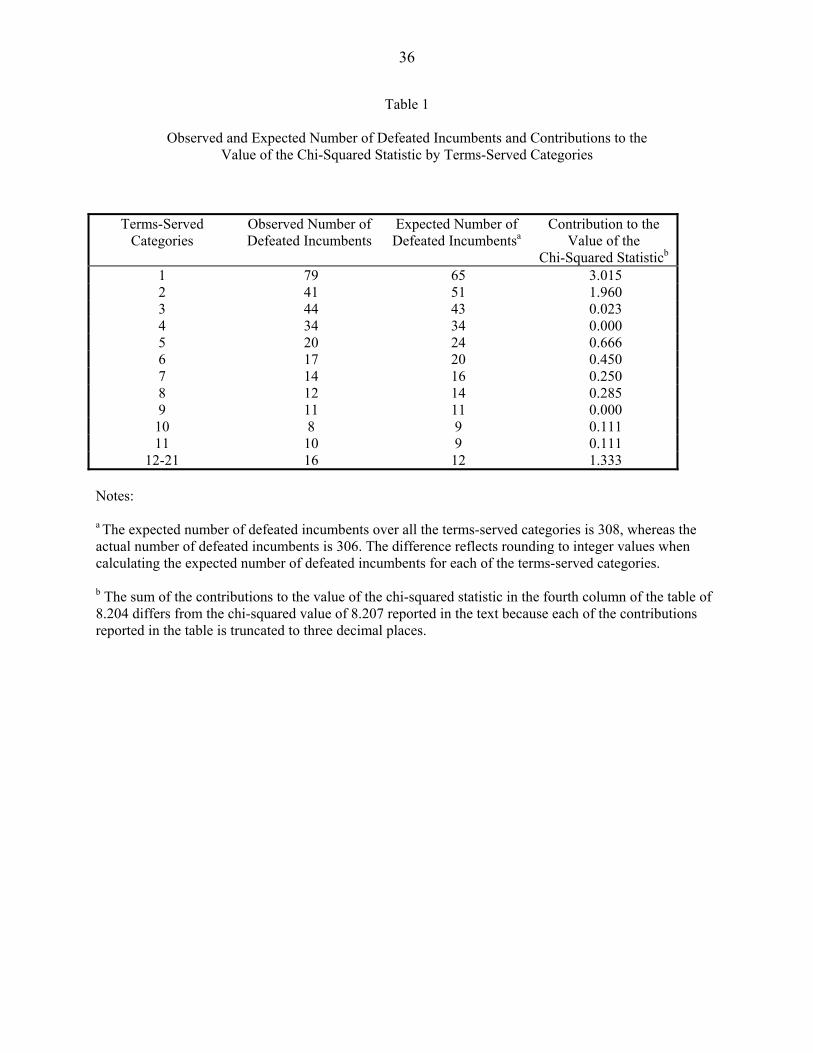
36

Table 1

Observed and Expected Number of Defeated Incumbents and Contributions to the Value of the Chi-Squared Statistic by Terms-Served Categories

Terms-Served Categories

Observed Number of Defeated Incumbents

Expected Number of Defeated Incumbentsa

Contribution to the Value of the

Chi-Squared Statisticb

1 79 65 3.015 2 41 51 1.960 3 44 43 0.023 4 34 34 0.000 5 20 24 0.666 6 17 20 0.450 7 14 16 0.250 8 12 14 0.285 9 11 11 0.000

10 8 9 0.111 11 10 9 0.111

12-21 16 12 1.333 Notes: a The expected number of defeated incumbents over all the terms-served categories is 308, whereas the actual number of defeated incumbents is 306. The difference reflects rounding to integer values when calculating the expected number of defeated incumbents for each of the terms-served categories. b The sum of the contributions to the value of the chi-squared statistic in the fourth column of the table of 8.204 differs from the chi-squared value of 8.207 reported in the text because each of the contributions reported in the table is truncated to three decimal places.