shipment frequency of exporters and demand uncertainty
TRANSCRIPT

Shipment frequency of exporters and demand uncertainty
Gabor Bekesa, Lionel Fontagneb, Balazs Murakozya, Vincent Vicardc,∗
aInstitute of Economics, CERS-HAS - HungarybPSE-Paris 1,Banque de France and CEPII - France
cBanque de France - France
Abstract
Exporters react to the uncertainty of foreign demand by adjusting their shipmentvalue as well as their shipment frequency. The number of shipments - here proxied bythe number of months with nonzero exports - is an additional extensive margin allowingadditional flexibility to firms in serving distant markets. Larger uncertainty requiresfirms to increase their inventory holdings in order to reduce backorder costs. Using across section of detailed monthly French export data we study this additional marginof trade, focusing on the role of demand volatility. We show that larger volatilityis associated with both fewer and smaller shipments, but that the fall in the size ofshipments is smaller reflecting increased level of inventory holdings. We also show thatthe impact of uncertainty is magnified by the time needed to serve the destinationmarket from the production location. These findings are consistent with a simplestochastic inventory management model that links uncertainty of demand a firm facesin a given market to its decision on how to serve that demand.
Keywords: Gravity, transport costs, frequency of trade, inventory model, customs
data
JEL classification: D40, F12, R40
PRELIMINARY DRAFT April 2013
∗Corresponding author: Bekes: [email protected], Institute of Economics, CERS-HAS, Budaorsiut 45, Budapest, Hungary. We thank Zsuzsa Holler for excellent research assistance. The authorsgratefully acknowledge financial assistance from the European Firms in a Global Economy: Internalpolicies for external competitiveness (EFIGE), a collaborative project funded by the European Com-mission’s Seventh Framework Programme (contract number 225551). Bekes thanks the hospitality ofCEPII. This paper represents the views of the authors and should not be interpreted as reflecting thoseof Banque de France or the European Central Bank. The entire responsibility for errors and omissionsremains on us.

1. Introduction
How many Barbie dolls should you ship from your Chinese assembly line to the UKfor next Christmas? This question illustrates uncertainty on demand (children mightprefer electronic devices this year) aggravated by distance (Guangzhou to Southamptonis up to a 30 days sailing route) and inventory costs. Posting new orders in case ofunderestimation of demand will be very costly (air delivery), while ordering more thandemanded means storing unsold dolls till next year. Hence, uncertainty faced by thefirm is positively affected by the uncertainty of demand and the time to ship (aggravatedhere by the seasonality of demand). Many more examples of seasonal business couldillustrate these general principle, as for example fertilizers whereby producers mustbuild inventories to allow for timely availability during the peak season.1 The problemfor producers is always to minimize the inventory cost, while keeping the option ofserving its usual consumers if the demand peaks.
Seasonality issues are an extreme case of a more general optimization problem facedby firms contemplating how to best serve their clients.2 When deciding on servingcustomers, firms make decisions on the size of likely sales and on the modes and detailsof how to best serve clients. When clients are close to production and/or there is noneed for delivery and storage, the second decision becomes less important, and a salemay be followed by another one (conditional on time to produce) after the first dealis closed. However, this is not the case when clients are far away or storage is neededto serve retail clients. Accordingly, foreign trade, where clients are located at largedistance from the supplier provides a laboratory where to study such decisions madeby firms in presence of demand uncertainty.
From a general economic perspective, international exchange is thus a good labora-tory to study how firms adjust their sales technology in presence of uncertainty, usingfrequency of delivery as a margin of adjustment. From a trade perspective, shipments isanother margin of exports worth studying: the question is neither whether you export(extensive firm margin), nor how much you export (intensive margin), but how often
1According to a report on a fertilizer company, sales vary significantly from one year to the next
due to weather-related shifts in planting schedules and purchasing patterns (Industries Holdings, INC
(2008) Source wikinvest.com). It is noted that when seasonal demand exceeds projections, customers
may purchase from competitors, and profitability will be negatively impacted. On the other hand if
seasonal demand is below expectations, the company will be left with excess inventory to be stored
and paid for and/or liquidated at a low price. Very long storage is also impossible in this business.2Trade technology depends on the route: air, land, maritime. According to Hummels (2009), three-
quarters of world trade involves countries that do not share a border and involves mostly maritime
transport. The mean cost of logistics as a percentage of the value of imports (all exporters) is in the
range of 5% to 10% for an American importer. It is noticeably lower in the US (4.5%) according to
Hummels (2009) calculations, than in smaller countries like Ecuador (9.2%). Part of the difference is
due to the non-freight costs (e.g. insurance, warehouses), that represent only 15% of the total for the
US but 55% for Ecuador.
1

you export, conditional on your foreign sales.3 How uncertainty affects the numberof shipments and their size is however a complex issue. Larger sales will increase thenumber and size of shipments (in proportion to be defined). Uncertainty on foreigndemand will reduce total sales due to the storage costs afore mentioned. Uncertaintywill also reduce the frequency of shipment, due to the sunk costs of shipping. Finally,uncertainty on foreign sales should reduce sales and thus the shipment size, thoughreducing the frequency of shipment and increasing the shipment size. What is the neteffect on shipment size remains an open question.4
These questions are particularly relevant for international exchange since there isno just-in-time when products have to be trade internationally. When time matters,firms can optimize transport by choosing between modes of air and maritime cargo(Harrigan 2010, Hummels and Schaur, AER forthcoming).5 Harrigan and Evans (2005)argue that an additional adjustment path is location choice: products that need tobe served at a timely fashion will be produced closer to destination markets, thusaffecting specialization patterns.6 We will consider that location choices are given, andaddress firms’ strategies conditional on these choices (we will look at export data forone exporting country only), and consider as a robustness maritime routes only.
In order to study this new margin of exports, we use the highly disaggregated natureof monthly export data for individual exporters and consider a new margin of trade: thefrequency of shipments. The transaction margin has already been observed in the tradeliterature, but receive limited attention (Eaton et al., 2008; Ariu, 2011).7 We use data
3Firms can also adjust by shipping different set of or products and/or to a different set of des-
tinations. Iacovone and Javorcik (2010) examine how uncertainty affects trade patterns considering
product level dynamics within firms for Mexico. The margin on adjustment here falls on products
and uncertainty leads to product churning and limited value for new flows. In these cases, experience
discussed by Araujo and Ornelas (2007) and Albornoz et al. (2012) help explain exporters’ behavior.
We will here focus on product-destination decisions: we assume that firms have already chosen their
portfolio of exported product to each destination.4We deviate from the literature (Hornok and Koren, 2012; Hummels and Schaur, forthcoming) by
focusing on the supply side and firm level maximization in the presence of simple demand function.
More precisely, we concentrate on logistics decisions and hence, the cost function of transportation,
rather than organizational decisions.5Indeed, as Hummels and Schaur (2010 JIE) demonstrated, uncertainty of demand will affect
transport behavior, in the presence of higher demand uncertainty, a greater share of shipments will be
taking place via air transport. We will address this issue by restricting our estimations, in a robustness,
to maritime transport.6Uncertainty is indeed impacting many other dimensions of individual firms decisions, like invest-
ment in presence of irreversibility (Bloom and Van Reenen, 2007), in line with the traditional real
option argument (Dixit and Pindyck, 1994). We focus here on trade models.7When analyzing Colombian transaction-level data, Eaton et al. (2008) show that the distribution of
number of transaction is highly skewed, and that the transaction contributes to total trade significantly.
Ariu (2011) also decomposes trade using the number of transactions using monthly trade data for
Belgium and finds the transaction margin to be important at both the firm-level and country level
2
from the French Customs at individual exporter level, providing monthly firm exportdata by destination and product category. Products are aggregated at the 6-digit levelof the Harmonized System (HS6), and shipment frequency is defined as the number ofmonths with non-zero shipment per annum for a given firm-product-destination. We usethe most recent pre-crisis year of observation (2007) and study the frequency of shipmentfor this cross-section for sake of tractability. However, uncertainty measurement willexploit the longitudinal dimension of the data. We limit our analysis to extra-EUexports in order to consider only relationships involving shipments of non-negligibleduration.
One important issue here is how to best measure uncertainty faced by exporters.We consider that due to stochastic demand, firms are unaware of the final demand andhence, face uncertainty. This definition is related to business dynamics, although all as-pects of a market may influence certainty of sales. To this end, we measure uncertaintyby averaging volatility of firms’ past (annual) sales changes for each product-destinationmarkets before the year considered, meaning over the period 1999-2006. Several studiesconsidered uncertainty, stemming from productivity shocks (Bloom et al. 2012), pricevolatility (Hummels and Schaur 2010 JIE) or instability of political-institutional vari-ables (Handley and Limao 2012). Our approach to uncertainty is somewhat different, aswe directly consider volatility of sales, and its use will complement existing approaches.
We firstly run firm-product-destination level regressions in a simple gravity frame-work to study how this margin of trade is used by firms to smooth the impact of busi-ness conditions on their different markets. We observe the adjustment of the numberof shipments and the size of shipments using firm-product fixed effects. Accordingly,we control for the composition effect as firms endogenously choose destinations andproducts to ship. We observe that the adjustment to market size is roughly channeledhalf trough the number of shipment and half trough their size.
In a second step, we study the impact of uncertainty on sales, number and size ofshipments. We find that: i) firms adjust on both margins to an increase in demand, andthis is mirrored in the (similar) elasticity of trade frequency and value per shipmentwith respect to demand; ii) higher uncertainty reduces export value, the number ofshipments and has an ambiguous impact on the average value of shipments; iii) holdingexport value fixed, higher uncertainty reduces the number of shipment and increasesthe average value per shipment; iv) the effect of uncertainty is magnified by shipmenttime: uncertainty only matters if transport is timely.
Finally, we show that these stylized facts are fully consistent with a simple theo-retical setting fitting inventory costs. Inventory models have been long used in logistictheory. More recently, they have been shown to be useful frameworks when explain-ing the impact of large demand shocks in presence of transaction and inventory costs(Alessandria et al., 2011). The models in Alessandria et al. (2010) and Alessandria
decompositions.
3

et al. (2011) were designed to explain time series evidence after large trade shocks.They consider a dynamic version of problem when the importer has to decide aboutimporting or not. They compare non-importers and importers in terms of reaction tofluctuation of condition, on the basis that importers take more time to adjust. Instead,our simple and tractable approach will reflect the inventory decisions of a firm exportingto many markets, and predict differences across markets and products.8
Against this background, we show that a simple model focusing on uncertainty,where firms pay per shipment cost to reach their foreign clients, and pay a storage costto store goods and serve clients as they appear, will easily reproduce our stylized facts.Note that inventory model’s predictions that shipment frequency will depend on sales,fixed costs and inventory costs are not unique. In Hornok and Koren (2011), consumershave heterogeneous preferences for the arrival time of a non-storable product and firmscompete by selecting the time of their shipment. Per shipment costs reduce shipmentfrequency and increase the shipment size and the product price. The preferred shipmenttime of the consumer also contributes to inventory costs. In case of demand uncertainty,a firm may sell some amount with doing another shipment if and only if the first batchis sold. Also, on explicit modeling of trade technology, see Behrens and Picard (2011)or Kleinert and Spies (2011).
In what follows, in Section 2 we first introduce our data, then provide some basicstatistics on shipment frequency as a margin of trade. The next section addressesthe impact of uncertainty on these export margins. We then rely on main alternativemeasurement strategies and results in a robustness section (additional robustness checksare relegated to the Appendix). Finally, a simple model of inventory management ispresented offering some testable predictions in Section 5. The last section concludes.
2. Data and descriptive stats
2.1. Data
We use detailed firm export data from the French Customs for 2007, providingmonthly firm export value by destination and product category at the 6-digit HS level9.Two different thresholds apply to the collection of French exports, depending on theircountry of destination. All extra EU export shipments over 1000 Euros are to bedeclared to the French Customs whereas for exports to other EU Member states thedeclaration is compulsory if the yearly cumulated value of exports to the other 26 EU
8Inspired by the Great Recession, Novy and Taylor (2013) also investigates the role of macro
uncertainty on trade volumes. They relate a real option model of stochastic inventory management
to the trade reaction model of Bloom (2009) emphasizing the role of imported intermediate inputs.
Using monthly US import and industrial production data, they suggest a link between uncertainty and
macro-economic cyclicality.9We excluded Ships and Aircraft because these items are not exported through usual transport
technology but through self-propulsion.
4

Member states taken together is larger than 150,000 Euros. We therefore restrict oursample to extra-EU exports.
Annual GDP data are from the World Bank and distance come from CEPII TradeDataset. Data on the mode of transport at the frontier are from Comext, which detailsthe mode of transport of extra-EU trade by destination and HS6 digit level and differ-entiate between sea, rail, road, air, postal consignment, fixed transport installations,inland water transports or own propulsion. We use the information on the main modeof transport by market (product × destination) to identify shipments by sea from othermodes of transport.
2.2. Descriptive statistics
How frequently do firms export? We compute the number of months for which ashipment was recorded in a cell firm-HS6 product category-destination. Consideringonly non-zero observations, the median is two shipments per year (Table 1).10 Inter-estingly, the upper quartile is corresponding to five shipments only: choosing when toexport is really a choice to be made by firms. The corresponding strategy has manydimensions worth looking at.
Table 1: Descriptive statistics: median, mean, first and last quartile of the number of
shipments (2007)
Mean p25 Median p75
Total 3.7 1 2 5
UE27 4.6 1 3 8
extra UE 2.3 1 1 2
Large countries (GDP) 4.2 1 2 7
Small countries (GDP) 2.8 1 1 3
Large firms 4.3 1 2 7
Small Firms 2.8 1 1 3
Intermediate goods 3.8 1 2 6
Other goods 3.6 1 2 5
Firstly, different destinations will be served differently: in EU destinations that willbe disregarded in our econometric exercise, the frequency is higher: the median is 3shipments compared to one for extra-EU trade relationships). This higher frequencycan be driven by proximity (authorizing less costly shipments), by market size (largemarkets can be served more frequently), by type of products exported, or even by thecomposition of exporters. Considering market size, we observe that destinations with
10This does not exclude indeed more than one shipment in a month for a given firm, but we will
loosely associate month in which a shipment is recorded to “shipment”.
5

above the median GDP receive more frequent shipments than destinations below themedian.
Big players ship their products more often, which is in line with the predictions ofour model. This is confirmed by the data and even more visible in the last quartilewhere the mean number of shipments is seven for the large firms.
Just-in-time strategies embraced by many producers, combined with global valuechains, should lead intermediate products to be exported more often. This differenceis only weakly in the data.
In order to focus on non-neighboring countries, we stick to non-EU destinations. Wecan observe in Figure 1 that Extra-EU destinations (remote, more uncertain) exhibit adifferent distribution of the frequency of shipments, with a much larger concentrationon single shipments.
Figure 1: Frequency of shipments, number of months, 2007, all and extra-EU
010
2030
4050
60P
erce
nt
1 2 3 4 5 6 7 8 9 10 11 12Number of months (all countries)
010
2030
4050
60P
erce
nt
1 2 3 4 5 6 7 8 9 10 11 12Number of months (extra EU)
Notes: firm-destination-product (HS6) level. Source: French Customs, authors’ calculation.
2.3. Simple gravity of the frequency to export
We can now use a simple gravity framework to decompose the different margins ofexports at the firm-product level. Our aim her is to describe how this new margin of
6

trade behaves. It is important as this margin is used by firms to smooth the impact ofdifferent business conditions on their different markets.11
Our first dependent variable is the log value of firm-product exports to each des-tination, for 2007. It is decomposed into the number of shipments per firm-producton each destination, and the mean value of these shipments for this firm-product. Wehave 568,131 observations for 315,659 firm-products.12 Remind that we consider onlyextra-EU destinations. In this elementary gravity framework simply aiming at provid-ing a decomposition of the margins at stake, we consider only market size (GDP of thedestination country) and distance from France (distances were taken from the CEPIIdatabase) as determinants of the value of firm-products exports. Indeed unobservedproduct and firm characteristics have to be controlled for, which is done in columns(2), (4) and (6) with firm-product fixed effects. All variables are taken in logarithmand the estimated coefficients on the mean value and the number of shipments add tothe coefficient on the total value in column (1). We cluster by destination-product. Allestimated parameters are significant at the 1% level.
Comparing columns (1) and (2), Table 2, we observe the traditional sorting offirms on remote destinations: when firm-product characteristics are not controlled,distance has a positive impact on the value of exports, which channels through theaverage value of the shipments in column (5). Big and more efficient players exporttheir better products on remote markets. Indeed, this composition effect disappearswhen controlling for firm-product characteristics in Columns (2) and (6). Demand hasultimately a positive impact on firm-product exports.
This simple framework makes it possible to decompose the two margins we are in-terested in: the number of shipments (more precisely the number of months a shipmentwas recorded for a given firm-product to a destination within a year) and the meanvalue of each shipment (more precisely of monthly exports of a given firm-product toa destination within that year). Considering the fixed-effects specification, we observethat more than half of the increase in exports to larger markets channels through themean value of shipments, less than half of impact of demand channeling through thenumber of shipments. Larger markets offer economies of scale in terms of logistics, asthe number of shipments increase less than demand. As for the impact of distance,three fourth fall on the number of shipments, and one fourth on their mean value.
11This baseline regression result (Table 2 ) is presented for the same sample as used for the rest of
the paper to ease comparability. Estimation details will be presented in section 3.12We use here the censored dataset, as in the follow up of the paper.
7

Table 2: Gravity variables and export margins
(1) (2) (3) (4) (5) (6)
value (log) nbr of shipments (log) avg value (log)
GDP (log) 0.032*** 0.167*** 0.013*** 0.070*** 0.019*** 0.097***
(0.003) (0.004) (0.002) (0.002) (0.002) (0.002)
distance (log) 0.087*** -0.099*** 0.009*** -0.075*** 0.078*** -0.025***
(0.006) (0.004) (0.002) (0.002) (0.006) (0.003)
Constant 7.724*** 5.705*** 0.042 -0.780*** 7.683*** 6.485***
(0.096) (0.099) (0.051) (0.051) (0.072) (0.059)
Firm*product fixed effect - Yes - Yes - Yes
Observations 568,131 568,131 568,131 568,131 568,131 568,131
Number of id 315,659 315,659 315,659
R-squared 0.006 0.045 0.002 0.041 0.005 0.026
Robust standard errors in parentheses
*** p<0.01, ** p<0.05, * p<0.1
Clustered by destination/product
3. Uncertainty and trade margins
This section studies how uncertainty affects export sales and the related margins –number and mean size of shipment – at the firm-product-destination level.
An important issue is accordingly the definition of uncertainty. Our preferred un-certainty variable is a proxy for the variance of the distribution of demand from ourmodel. It captures the average uncertainty of sales faced by French firms on a specificmarket (j, k) when deciding to ship, i.e. the distribution of sales variations over timeon the market.
More specifically, uncertainty is measured as the cross-firm average standard devia-tion of firms’ yearly export growth at the product and destination level over the period1999-2006. High uncertainty reflects a higher volatility of the demand addressed tofirms and may be related to both variations in overall annual demand on the marketand/or the process of reallocation of market shares across firms.
equation here
Robustness estimations with alternative measures of uncertainty are provided in thenext section.
3.1. Estimation strategy
In terms of methodology, let us emphasize a few important issues: restriction ofcountries, panel structure, using fixed effects and dummies to instead of cost estimates
8

and censoring. Robustness checks will be discussed in a separate section.
Restriction of countries. Importantly, we dropped all EU countries from the samplefor two reasons. First, shipments within the EU are recorded differently, and we loosemany smaller shipments. Second, transport within the EU is mostly swift and timeand distance plays a much smaller role. A robustness check including EU countries ispresented in available on request.
Panel structure In particular we will relate uncertainty to (1) total (annual) ship-ment value (val tot), (2) shipment frequency (freq), (3) average shipment value (val avg).All dependent variables (value, number of shipments and average value) are presentedin logs and estimate model at the at firm-product-destination (i, j, k) level yields:
V alueijk = α + β1vYk + β2vDistk + β3vUncertjk + θij + εijk (1)
NbrShipijk = α + β1fYk + β2fDistk + β3fUncertjk + θij + εijk (2)
AvgV alijk = α + β1aYk + β2aDistk + β3aUncertjk + θij + εijk (3)
Our data is firm-product-destination level panel (for one year). These equationsmay be estimated by OLS but we included θij product-firm fixed effects to controlfor composition effects as well as unobserved cost characteristics. Selection is reallyimportant as more productive firms self-select into different countries, as they are theones that can pay the sunk of exports to harder markets (Mayer and Ottaviano, 2011;Arkolakis, 2010). Furthermore, Bekes and Murakozy (2012) argue that more productivefirms will more likely export at a permanent (and hence, more frequent) fashion. Notethat adding firm-product FE implies that single-product, single-destination (outsidethe EU) exporters are not considered.
To handle the fact that error terms may be correlated we cluster standard errorsby the dimension of our key uncertainty variable (product * destination). To controlfor unobserved country characteristic, for several estimations, GDP and distance arereplaced with country dummies. This allows us to focus on product-country leveluncertainty.
Parameters and dummies This paper focuses on the impact of uncertainty on ship-ment behavior13. Per shipment fixed costs may include per container costs, adminis-trative cost at the border, insurance and distribution. Inventory cost would includewarehouse costs that are shaped by size and weight, specific conditions for perishablegoods, as well as firm specific effects (e.g. financial strength that may affect the dis-count rate). Both per shipment costs and storage costs are very hard to measure - andinstead, we’ll argue that firm-product fixed effects will also control for these costs.
13An earlier working paper version includes a greater set of variables.
9

At a later stage, we introduce destination specific fixed effects that shall pick costsassociated with destination market interest rates, as well as doing business types ofcosts of each shipment. As the identification is on the cross section, these fixed effectsshall control for most variables of the model apart from the product-destination specificuncertainty, the effect of which we look for14.
Censoring As presented in section 2.2, the number of shipments is censored at twelve(months). One of our concerns is that the number of months is a noisy proxy of thenumber of shipments in a given year. While it is a reliable approximation for lowfrequency exports, it may be biased for frequent exporters. To handle this problem, weopted for the simplest treatment and dropped the upper tail of the distribution focusingon firm-product-destination observations for 1-9 shipments. In terms of generality, thisis not a very serious problem, as this requires dropping only 6 percent of observations.
Results for the uncensored sample are presented in the Appendix15 According touncesnored results, our benchmark censored results, apart from reducing the effectof the bias, also reduce the strength of the transaction adaptation channel. Hence,censored results show more conservative estimates.
3.2. How margins adjust to uncertainty
The first two stylized facts that we will show refer to the margins of trade and theimpact of uncertainty. This is also shown in Table 2.
Table 3 presents results for our baseline regressions for OLS (cols 1,3 and 5) as wellas firm-product fixed effects regressions (columns 2,4 and 6). The dependent variablefor the first two columns is the log of annual sales, followed by two columns on lognumber of shipments (months) and then, log average value.
Results show that estimated GDP coefficient is approximately equally divided be-tween frequency and average size: 0.016 vs 0.018 for the OLS and 0.071 vs 0.096 forthe firm-product FE model. Note that relationship is also present in Table (12) wherewe use the broadest possible sample and present simple uncensored results (0.038 vs0.046 for the OLS and 0.102 vs 0.135 for the FE model). Accordingly, our first stylizedfacts is that firms equally adjust the number of shipments and their size to observablechanges in demand.
The second stylized fact is that higher uncertainty reduces shipment value as wellas the shipment frequency. This is illustrated in three specifications: pooled OLS(columns 1,3,5 of Table 3), firm-product fixed effects (columns 2,4,6 of Table 3), and
14One can expect that products with high depreciation rate (perishables) react differently. Unfor-
tunately food items, which is a clear candidate, is also seasonal and as France ships little raw food
overseas, is not a convincing candidate. Fast fashion is hardly distinguishable at 6-digit level. Instead
we tried intermediate goods (by BEC category) as shipping these goods are rather time sensitive.
There was no apparent difference.15All results presented are confirmed (available on request) when we restrict sample for 10 and below
or 8 and below shipments as well.
10

Table 3: Baseline regressions
(1) (2) (3) (4) (5) (6)
value (log) nbr of shipments (log) avg value (log)
GDP (log) 0.034*** 0.167*** 0.016*** 0.071*** 0.018*** 0.096***
(0.003) (0.004) (0.002) (0.002) (0.002) (0.002)
distance (log) 0.087*** -0.100*** 0.010*** -0.075*** 0.078*** -0.025***
(0.006) (0.004) (0.002) (0.002) (0.005) (0.003)
uncert (log) -0.068*** -0.023** -0.146*** -0.055*** 0.078*** 0.032***
(0.013) (0.009) (0.006) (0.004) (0.010) (0.007)
Constant 7.699*** 5.694*** -0.013 -0.807*** 7.712*** 6.501***
(0.095) (0.101) (0.046) (0.051) (0.073) (0.060)
Firm*product FE - Yes - Yes - Yes
Observations 568,131 568,131 568,131 568,131 568,131 568,131
Number of id 315,659 315,659 315,659
R-squared 0.006 0.045 0.009 0.042 0.006 0.026
Robust standard errors in parentheses
*** p<0.01, ** p<0.05, * p<0.1
Clustered by destination/product
11

firm-product fixed effects as well as destination dummies (table 4). Note that themeasured effect of uncertainty is very different when we control for the compositioneffect.(i.e. the difference between OLS and firm-product FE). The coefficient of thetotal volume falls substantially (by about two-thirds) when we control for firm andproduct characteristics. This is then affects both shipment frequency and average size,about equally in magnitude.
Considering our preferred destination FE specification (Table 4), a firm facing a10% higher uncertainty for a given product at a given market is selling 0.7% less atthat market, with most of the hit taken through fewer (0.5% less) number of shipments.
Note that the full effect on average shipment size is negative but this result isstrongly dependent of specification and control. The relationship between uncertaintyand average value can go either way depending on relative size of various types of costs.
Comparing Table 4 to Table 3, the impact on sales and number of transactionsremain in the same magnitude as before. The coefficient of the average shipment sizebecomes negative suggesting that the effect of declining overall sales is not fully passedthrough on the size of shipments, when additional controls are employed. The destina-tion FE specification is our preferred model, and hence, from now on, all specificationswill include firm-product as well as destination fixed effects unless otherwise indicated.
Table 4: The role of uncertainty: destination fixed effects
(1) (2) (3)
value (log) avg value (log) nbr of shipments (log)
full sample full sample full sample
uncert (log) -0.072*** -0.020*** -0.053***
(0.009) (0.007) (0.004)
Firm*product FE Yes Yes Yes
Destination FE Yes Yes Yes
Observations 568,131 568,131 568,131
Number of id 315,659 315,659 315,659
R-squared 0.060 0.050 0.058
Clustered by destination/product
Both Table 3 and table 4 presented results on the censored sample. As we willshow in the next sub-section, all variable estimates are on the conservative side, withestimated coefficients on both total value and number of shipments typically doubledwhen using the full sample.
12

3.3. Adjustment of margins conditional on sales
So far we have considered unconstrained models. The number of shipments willalso fall because even for the same amount of sales, firms will choose to send fewershipments when uncertainty is high (exactly the opposite for package size). We runthe same regression as before, but for this constrained version, we control for the totalvalue, and 2 becomes:
NbrShipijk = α + β1fYk + β2fDistk + β3fUncertjk + β4 V alueijk + θij + εijk (4)
Results in Table 5 confirm this: when we compare two shipments controlling forthe annual total volume, the product-destination market with 10% higher uncertaintyis associated with 0.3% less transactions. (Coefficients on the average size is exactlyopposite when total sales are controlled for.) Thus, we can see that the about halfof the drop in transport frequency come from the firm’s optimization effort yieldingless overall sales, while the other half comes from less frequency for less the same sales(0.03% vs 0.053%).
Table 5: Role of uncertainty conditional on sales
(1) (2) (3)
avg value (log) nbr of shipments (log) nbr of shipments (log)
full sample full sample Maritime only
uncert (log) 0.030*** -0.030*** -0.028***
(0.003) (0.003) (0.003)
total value (log) 0.684*** 0.316*** 0.325***
(0.001) (0.001) (0.001)
Constant 2.202*** -2.202*** -2.235***
(0.016) (0.016) (0.032)
Firm*product FE Yes Yes Yes
Destination FE Yes Yes Yes
Observations 568.131 568,131 300,906
Number of id 315.659 315,659 170,273
R-squared 0.811 0.495 0.499
Clustered by destination/product
Of course, total sales is fully endogenous as a control for number of shipments.To treat this endogeneity, we instrument value by market size - measures as the globalimports to a given product-destination pair using data from the COMTRADE dataset16.
16Our data coming from French customs is 86% correlated with COMTRADE data on imports from
13

Results hold when instrumenting value by total imports, or even when simply replacingthem.
3.4. Impact of uncertainty magnified by distance
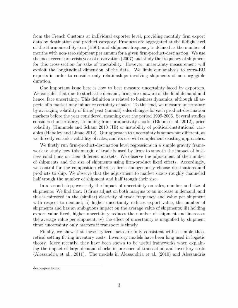
Table 6 tests the argument that distance (travel time) magnifies the effect of uncer-tainty. To test this, we interact our distance and uncertainty variables, so add a crossterm of uncertainty and distance to equation and and 2 becomes:
NbrShipijk = α+β1fYk+β2fDistk+β3fUncertjk+β4Distk ∗Uncertjk+θij + εijk. (5)
Columns 1-2 present basic results, columns 3-4 includes the control of total values aswell. Our model is specified for maritime travel in mind, involving a great deal of timefor a shipment. However, we have analyzed the whole sample (of non-EU countries)so far. However, even for overseas (or far away countries that may be reached both byroad and shipping, such as Russia), some part of the transport is carried out by air orroad. This may explain the lack of results in column 1.
Fortunately, for 52% of our sample, we know that transport include maritime trans-portation - with rest including air, road, and unidentified. Indeed, this instance, thetravel mode distinction becomes important, as the cross term is estimated to be non-zeroonly for the maritime (ie certainly time consuming) modes of transport. The coeffi-cient of uncertainty is estimated to be positive, but for all markets beyond 7000km,the combined effect is negative. A possible non-linearity of this relationship is testedby employing three dummy variables in columns 5 with results suggesting the negativeeffect to be in place for 8000km and beyond.
4. Robustness
We analyze here the robustness of our findings using alternative estimation methods,alternative measures of uncertainty and finally tackling more minor issues.
4.1. Alternative estimation methods
Robustness results are presented in Table 7. Regression results here include countrydummies with additional robustness checks with GDP and distance relegated to theAppendix. Column (1) reproduces column (3) from Table 4 to ease comparability.Column (2) shows baseline results for whole sample, ie. including observations withshipments 10-12. The estimated coefficient is higher (-0.053 vs -0.088), and this remainstrue for other specifications. In the Appendix we present a Table 12 with full sampleresults for selected models, and additional results are available on request.
France.
14
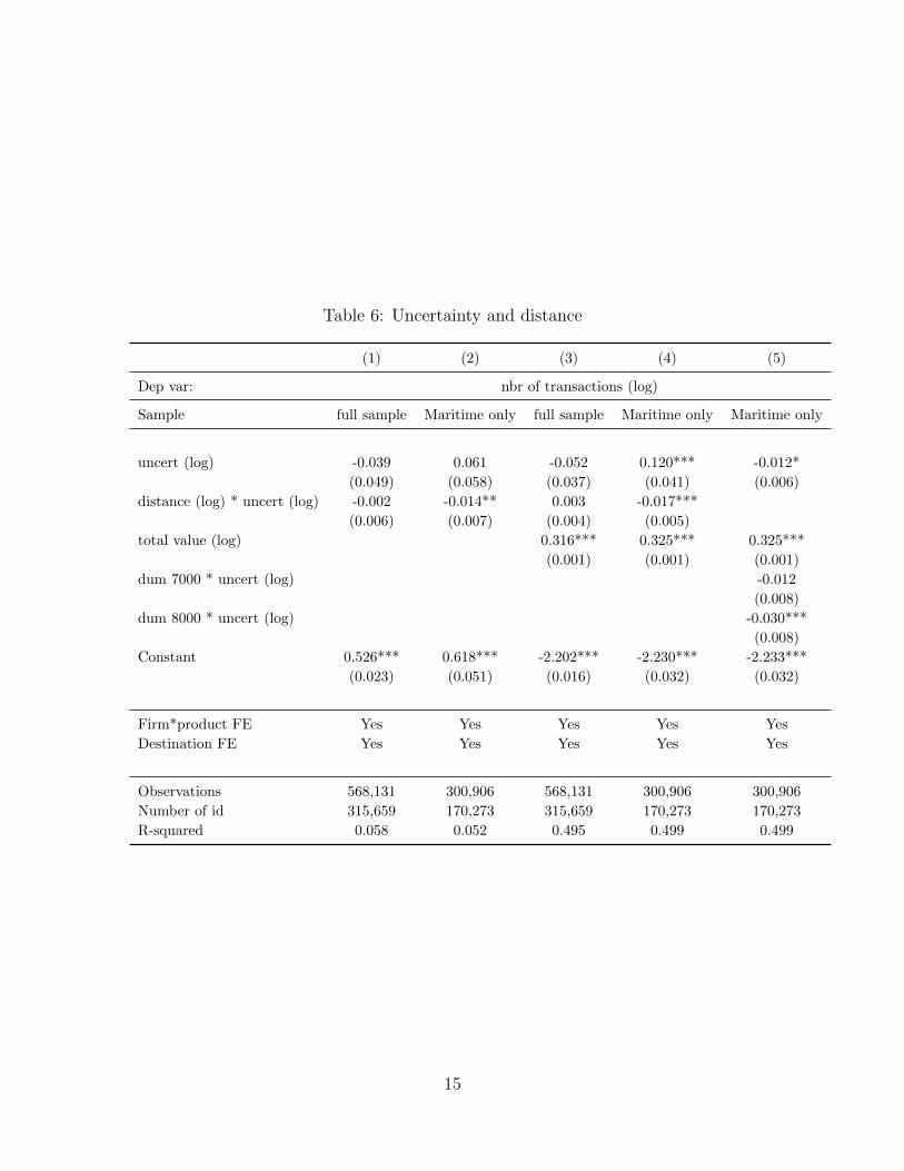
Table 6: Uncertainty and distance
(1) (2) (3) (4) (5)
Dep var: nbr of transactions (log)
Sample full sample Maritime only full sample Maritime only Maritime only
uncert (log) -0.039 0.061 -0.052 0.120*** -0.012*
(0.049) (0.058) (0.037) (0.041) (0.006)
distance (log) * uncert (log) -0.002 -0.014** 0.003 -0.017***
(0.006) (0.007) (0.004) (0.005)
total value (log) 0.316*** 0.325*** 0.325***
(0.001) (0.001) (0.001)
dum 7000 * uncert (log) -0.012
(0.008)
dum 8000 * uncert (log) -0.030***
(0.008)
Constant 0.526*** 0.618*** -2.202*** -2.230*** -2.233***
(0.023) (0.051) (0.016) (0.032) (0.032)
Firm*product FE Yes Yes Yes Yes Yes
Destination FE Yes Yes Yes Yes Yes
Observations 568,131 300,906 568,131 300,906 300,906
Number of id 315,659 170,273 315,659 170,273 170,273
R-squared 0.058 0.052 0.495 0.499 0.499
15

This is followed by two random effect effect models - one simple way to treat poten-tial over-specification (Matyas, Hornok, Pus 2012). Results confirm earlier results whileshowing a coefficient estimate somewhat larger than before. We carried out truncationin this case as well, with no apparent change. In the in column (5) we present resultswith a Tobit model, in which all observations with more than 8 months are treated ascensored17. Once again, the key negative relationship between shipment frequency anduncertainty is confirmed.
Table 7: Different estimators
(6) (7) (8) (9) (10)
nbr of shipments (log)
OLS Fixed Effects OLS Random effects Tobit RE
Sample Baseline All transactions Baseline All transactions All transactions
uncert (log) -0.053*** -0.088*** -0.130*** -0.197*** -0.118***
(0.004) (0.005) (0.008) (0.009) (0.003)
Constant 0.526*** 0.626*** 0.548*** 0.629*** 0.537***
(0.023) (0.028) (0.018) (0.023) (0.010)
Firm*product FE Yes Yes - - -
Destination FE Yes Yes Yes Yes Yes
Observations 568,131 595,809 568,131 595,809 595,809
Number of id 315,659 319,068 315,659 319,068 319,068
R-squared 0.058 0.096
Robust standard errors in parentheses
*** p<0.01, ** p<0.05, * p<0.1
Clustered by destination/product
Looking at results at Table 7 as well as Table 12 we can see that point estimates of theuncertainty variable vary between -0.053 (our baseline estimate) and -0.217 suggestingthat presenting results on the truncated sample with destination fixed effects is a ratherconservative approach.
To reflect the potential inconsistency resulting from heteroscedasticity in data, weuse Poisson pseudo maximum likelihood estimator proposed by Santos Silva and Ten-reyro (2006). This methodology is consistent with average value of shipment estimationand the number of shipments proxied by the number of non-zero monthly exports - atthe firm-destination-product level. Poisson PML results - with destination fixed effectsare presented in Table 9 and Table 10 of the Appendix confirm key results (with theeffect of uncertainty on the total value being not significant).
17Changing the censoring limit to 8 or 10 months does not change the results importantly.
16

4.2. Alternative measures of uncertainty
Our benchmark measure looked at dynamics in a given (i, j) (i.e. product-destinationcountry) market. In this subsection, let us consider alternative measures to our uncer-tainty variable.
First, we consider uncertainty based on variation of demand over time. Firms maylook at demand uncertainty from the vantage point of overall demand fluctuations basedon past experience. To capture this, we created the uncertagg variable as the relativestandard deviation of quarterly sales (j, k) for 32 quarters (1999-2006). We added zerosto quarters when annual sales that year were non zero and applied a simple seasonaladjustment by calculating quarter dummies as deviations from a trend.
Both our benchmark and the uncertagg variables may be endogenous to the (i, j, k)shipment. To avoid this, our second alternative variable uncertaggita replaces relativestandard deviation overtime of French Firms, calculated by those experienced by Italianfirms. Of course, this means a great deal of loss of observations, as we can only observemarkets served by both French and Italian firms.
Our third alternative measure is a firm’s experience in a given market. As localexperience helps a firm know its market better, it can reduce uncertainty. A firm’s ex-perience in a given market (i, j, k) is simply the number of years with non-zero exportssince 1991. Of course this variable captures firm age and overall export experience.However, given our firm-product fixed effect specification, this shall be partially out.Please note that this variable has the opposite expected sign as all other, as a greaternumber represents more certainty while for other variables, it implies greater uncer-tainty.
Results, looking at both total value and the number of shipments, are presented inTable 8, comparing the effect to the benchmark case, one by one, and finally taking thebenchmark, the aggregate and firm experience variables all together. Table 8 presentsresults: Panel A for total value, Panel B for number of shipments, Panel C repeats theexercise for average number of shipments. All results presented before are confirmed asall uncertainty variables behave the similar way as our benchmark.
17

4.3. Additional robustness checks
We made several additional robustness checks: looking at a smaller sample of firms,dropping small markets, and focusing on a set of products whereas classification hasbeen stable.
Firms We considered robustness from another angle: the sample of shipments con-sidered. As discussed before, the first point was to reduce the sample for maritimeshipments, than we considered manufacturing firms only, and finally incumbent firms,ie those who exported the same product to the same destination. Results, presented inthe Appendix (Table 12), confirm earlier results.
Market sizen About 1/3 of product-destination markets are served by only one firmat a time. In this case, volatility is identified from past sales of this firm. As robustnesscheck, we dropped all observations to these markets (reducing sample size from 595K to522K), and repeated all regressions. We found marginally higher estimated uncertaintycoefficients, and hence, if anything, we have underestimated the impact of uncertainty.Results available on request.
HS6 coding stability. There has been many coding changes in the HS6 classification.This is is not random, as more technology related products are recoded. Hence, wedropped all codes that went through any change between 1999 and 2007 - affectingabout 20% of total observation. Results suggesting that this had no effect, are availableon request.
18

Table 8: Alternative uncertainty measures
Panel A
Dep value (log)
uncert (log) -0.066***
(0.011)
uncertagg (log) -0.241***
(0.010)
uncertaggita (log) -0.033***
(0.005)
Experience by dest*prod 0.076***
(0.001)
Constant 8.629*** 8.480*** 8.631*** 8.254***
(0.057) (0.058) (0.056) (0.057)
R-squared 0.057 0.063 0.057 0.081
Panel B
Dep nbr of shipments (log)
uncert (log) -0.052***
(0.005)
uncertagg (log) -0.145***
(0.005)
uncertaggita (log) -0.020***
(0.002)
Experience by dest*prod 0.044***
(0.001)
Constant 0.507*** 0.418*** 0.509*** 0.290***
(0.029) (0.031) (0.029) (0.029)
R-squared 0.058 0.066 0.058 0.094
Panel C
Dep avg value (log)
uncert (log) -0.014*
(0.008)
uncertagg (log) -0.096***
(0.007)
uncertaggita (log) -0.012***
(0.004)
Experience by dest*prod 0.032***
(0.001)
Constant 8.121*** 8.062*** 8.122*** 7.964***
(0.036) (0.036) (0.035) (0.036)
R-squared 0.048 0.050 0.048 0.056
For all panels, a unified sample is used: number of observation is 507,930, number of id is 291,127.
Robust standard errors in parentheses, clustered by destination/product.
Product-firm FE and destination dummies always included.
19

5. Modeling shipment frequency
We illustrate here that the stylized facts afore mentioned can be reproduced using asimple model of steady state behavior. One can easily describe how trade frequency (thenumber of shipments per year by a firm from one product to a given country) changeswith demand parameters and uncertainty about demand with explicitly accounting forlogistical/operation management decisions of firms. In this setup firms consider externaldemand at each of their (product-destination) markets and optimize their shipmentprocess based on available cost information as well as uncertainty about demand.
We consider here the total logistics cost, which includes transportation cost, per-shipment costs as well as warehouse expenses. We investigate a direct exporter, andassume that the firm pays all transportation costs and sells to foreign clients directlyfrom its warehouse in the foreign country. Hence, retailers play no role in our framework.
In this section, let us first review a baseline deterministic model followed by astochastic version. This will be based on the review of Zipkin (2000). Having discussedcosts of inventory management, we turn to firm maximization and then summarizepredictions for the empirical work.
5.1. Deterministic demand
The starting point of our framework is the idea of inventory management, wherefirms optimize inventory decisions under different circumstances. The simplest suchmodels investigate the optimal policy under a constant demand rate, and hence, aredeterministic in nature.
In the deterministic framework, the firm faces a demand of λ in each time period,has to pay a per-shipment cost of k each time when placing an order, the variablecost of transportation is τ , and holding one unit of inventory costs h per unit of time.Inventory cost shall include all costs related to storage such as rent, running cost offacilities and personnel. Furthermore, it includes the cost of capital that covers thevalue of stored goods, which may be affected by the financial position of the firm. Inthe simplest case, the firm has to hold enough inventory to satisfy the demand of allcustomers from its holdings, hence quantity sold is exogenously determined.
The main decision variable is the average shipment size, which also determinesthe number of shipments per period. The tradeoff the firm faces is between moreshipments implying higher per-shipment costs and more inventory holding implyinghigher inventory costs. Under such circumstances, the firm minimizes its total logisticcost:
C(q) = τλ+ kλ/q + 1/2hq
where q is the average shipment size. Note that it is assumed that goods will bedepleted linearly and hence, average value of goods kept abroad is half the shipmentquantity. The optimal shipment size is:
20
q∗ =
√2k
hλ
while the optimal number of shipments is:
f ∗ =
√h
2kλ
Hence both the number of shipments and the quantity/shipment increases in pro-portion to the square root of demand intensity, λ. It is optimal to adjust to largermarket size on two margins: logistics costs are minimized when the firm increases boththe number of shipments and shipment size in proportion to the square root of demand,as both margins has a similarly increasing marginal cost schedule18.
Now we can express the total logistics cost (per period) of the firm:
C∗ = τλ+√
2kλ
which takes the general form of Bλ+C√λ. As we will see, this general form remains
valid in more realistic inventory models as well. Note that this formula suggests that- in contrast to iceberg trade costs - there are economies of scale in logistics thanks tothe presence of per-shipment costs.
A simple modification of this model enables firms to serve some customers withdelay. In the inventory literature this is called a planned backorder. Such plannedbackorders are costly to the firm either because consumer satisfaction is lower or becauseserving these customers requires some extra spending. We assume that the firm facesa penalty cost of b per backordered unit. It can be easily shown that the main resultsof the previous model are preserved in this case. First, both optimal shipment size andfrequency are proportional to
√λ :
q∗ =
√2kλ
h
√1
ω; f ∗ =
√hω
2kλ
where ω = bb+h
is the relative size of the backorder penalty. The total optimal
logistics cost also takes the form of Bλ+ C√λ :
C∗ = τλ+√
2kωλ (6)
One empirical prediction of this extension is that it allows one to analyse differencesacross perishable (food, fashion goods) and non-perishable products. The relative back-order cost of perishable products is much larger, leading to more frequent shipments,and also, ceteris paribus, to higher logistics costs.
18The model has a similar mechanics to the well known Baumol-Tobin model.
21

5.1.1. Stochastic inventory models
While deterministic inventory models are able to capture a number of importantaspects of real-world inventory problems, one of our main aims is to investigate therole of demand uncertainty explicitly. For this, one has to turn to stochastic inventorymodels.
In such models demand follows a stochastic process. While the models are able tohandle very general processes, we will concentrate on a normal approximation here.Assume that the demand (D) in a period with a length of T can be approximated witha normal distribution with a mean υ = E(D) = λT and variance σ2 = V ar(D) = ψ2λT .19 Note that the expected value of this process does not depend on time, hence it issuitable to describe steady state behavior. Describing other situtations, like dynamicadjustements to a large permanent shock may require other stochastic models.
As we will see, the key measure of uncertainty for the firm is the variability ofdemand between the actions of the firm and the arrival of the shipment. This is theproduct of the time required for the shipment to arrive and the volatility of demand.Note that if the shipment arrives instantly or demand is deterministic, then we are backto deterministic models - hence deterministic models can do a better job in describingtrade frequency between nearby countries than between far away trading partners.
The time needed for the inventory to arrive will be denoted by L. λ will show the(now stochastic) intensity of demand, while ψ2, the asymptotic variance-to-mean ratiorepresents the relative variability of demand.
We will also specify an inventory policy describing the behavior of the firm. Awidely used policy is the (r,q) model. This means that the firm always sends q unitswhenever the inventory declines below the re-order point, r. The optimization requiresfirms to to choose q and r optimally to minimize the expected logistics cost. In thisdecision the tradeoff between inventory costs and per-shipment costs is complicated bythe fact that low inventory levels may lead to larger expected backorder costs.
Unfortunately such models do not have a closed form solution in general. It can beshown, however, that in important respects the optimal policy is very similar to thatin the deterministic case.20 In particular, the behavior of lower and upper bounds forq∗, f ∗ and C∗ provides important clues about the shape of optimal policy21.
First, we have the following bounds for q∗:√2k
hωλ ≤ q∗ ≤
√2kω + bψ2L
hω2λ (7)
19This can be interpreted as an approximation of a Poisson demand process, with mean and variance
λT .20See subsection 6.5.3 of Zipkin (2000).21An important difference relative to the deterministic case is that these are expected values.
22

Taking logs22:
1
2ln
2k
hω+
1
2lnλ ≤ ln q∗ ≤ 1
2lnλ+
1
2ln
2k
hω+
1
2ln(1+
b
kωψ2L) ≤ 1
2lnλ+
1
2ln
2k
hω+
b
2kωψ2L
(8)
One observation is that both bounds increase proportionally with√λ, hence it is a
good approximation that q∗ increases linearly with√λ. Second, while the lower bound
is independent of ψ2L, the upper bound increases in it. The intuition of this result isthat the larger uncertainty is, the larger shipments the firm sends in order to reducethe expected value of backorders, leading to a smaller expected number of shipmentsconditional on λ. The above formula shows that this effect is zero when b = h, andbecomes stronger as the cost of backorders increases relative to inventory costs. All inall, it is possible to approximate ln q∗ with a relatively simple functional form:
ln q∗ ≈ Aq +1
2lnλ+ Cqψ
2L (9)
where Aq, Cq depend on b, h and k. Similarly, the optimal expected frequency,f ∗ = λ
q∗can be approximated by
ln f ∗ ≈ −Aq +1
2lnλ− Cqψ2L (10)
One can see that the important result of the deterministic case, that both frequencyand batch size increases linearly to the square root of demand.
The effect of uncertainty is less obvious. The main effect of increasing uncertaintyis that the expected cost of backorders increases for each level of inventories. Hence,when uncertainty increases, it is optimal to increase average inventory levels in order toreduce expected backorder costs. Optimizing firms do it on two margins: they increaseboth their reorder points and the average shipment size. Larger shipments result in lessfrequent deliveries for the same demand intensity.
Uncertainty also affects total logistic costs on three channels. First, it leads to largerexpected backorder costs. Second, as firms increase their inventory levels, inventorycosts also increase. These two effects are somewhat mitigated by a fall in per-shipmentcosts. Total logistics costs can be approximated by lower and upper bounds:
τλ+√
(2khω + b2Υ2(ω)ψ2L)λ ≤ C∗ ≤ τλ+√
2khωλ+ bΥ(ω)√ψ2Lλ
where Υ(ω) = φ(Φ−1(1−ω))1−ω and Φ, φ are the cdf and the density function of the Normal
distribution, respectively. Assuming that σ is relatively large23, we can approximate
22And applying the formula ln(1 + x) ≤ x23Zipkin (2000) p.219 provides numerical simulations showing that this approximation is valid even
for relatively small values of σ.
23

the cost function as
C∗ ≈ τλ+ (C1 + C2
√ψ2L)
√λ (11)
where C1 =√
(2khω) and C2 = bΥ(ω).
This result shows that in the stochastic case the cost function remains similar tothe one in the deterministic case in the sense that it is a linear function of λ and
√λ.
The new element is that the coefficient of√λ increases in demand uncertainty thanks
to larger expected backorder costs and the required increase in inventory levels: totallogistics cost is increasing in uncertainty, but less then proportionally.
Also, uncertainty is the product of the variance of demand (ψ2) and the time toship (L): if either of them is small, than logistics cost is not effected significantly bythe other one. This result is highly intuitive: the effective uncertainty the firm faces isthe variability of demand between its actions and the arrival of the shipment.
These observation lead to the important consequence that firms’ transportationcosts can feature strong economies of scale. While this is true in the deterministic case,the stochastic case shows that uncertainty even increase this nonlinearity through itseffect on the desired inventory level. The model predicts that both transportation costsand the economies of scale increase in demand uncertainty and distance.
The model is also able to capture the role of perishability resulting from non-durability of foods or fashion goods. One may assume that these goods depreciatequicker then durable goods, hence h is higher for these goods than for durable goods.For simplicity, we may also assume that the backorder cost is also higher for thesegoods to a similar degree (hence ω is the same for the two type off goods). In such acase, both the lower and upper bound goes down in 7. Hence firms send such goodsmore frequently but in smaller shipments. Perishability, however, is quite distinct fromuncertainty of demand in this framework.
5.2. Firm maximization
The previous models assumed that λ, (expected) quantity is given. When applyingthe model to real data, however, one has to take into account that market size anduncertainty affect the quantity choice of firms through changes in its marginal costschedule. Higher uncertainty, for example, leads to an upward shift in the marginalcost curve, implying smaller quantity sold.
Let we denote the market size in country i as Mi. The demand curve the firm facesin this country is λi = MiD(pi);
∂D∂λi
< 0. The cost function of the firm is the sum of itsproduction (ciλi) and logistic costs:
C(λi) = ciλi + τλi + (C1 + C2
√ψ2L)
√λ (12)
As noted above, this function features economies of scale, which are increasing inuncertainty. The firm maximizes its profit:
24

Πi = D−1(λiMi
)λi − C(λi) (13)
To get an intuition of comparative statics, note that the marginal cost schedule is:
MCi = ci + τ +1
2(C1 + C2
√ψ2L)
1√λ
(14)
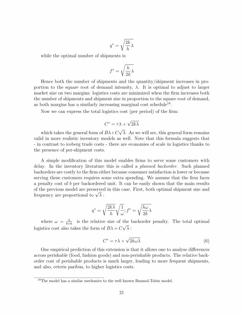
The marginal cost functions of two similar markets with different volatility is de-picted on Figure [2]: market 2 is more uncertain, hence marginal costs are higher onit for all quantity levels. As a comparison, the horizontal line represents the icebergtransportation cost case, when marginal costs are constant.
Let us analyze first the effect of increase in market size, shown in Figure 3. Here,the increasing returns of logistics leads to a larger change in the quantity sold andsmaller increase in price by the firm than under iceberg transportation costs. Hence,taking account inventory costs predicts a larger than proportional reaction of quantityto market size. As the elasticity of both shipment size and the number of shipmentswith respect to quantity is 1/2 in our framework, their elasticity with respect to marketsize can be somewhat larger than 1/2 thanks to the increasing returns of logistics.
Second, an increase in demand uncertainty tilts the marginal cost schedule. This isillustrated on (Figure 3), which compares two similar markets with different levels ofuncertainty. Uncertainty reduces quantity sold, and the effect depends on the elasticityof demand and the slope of the marginal cost curve.
When analyzing the effect of uncertainty on shipment size and the number of ship-ments, we should combine this observation with the previous result that - with fixedquantity - uncertainty leads to larger and less frequent shipments. Hence, we expectthat uncertainty leads to a decrease in frequency on two channels: first, it leads to afall in quantity, and hence, to a decrease in frequency; second, it leads to less frequentshipments even when quantity is unchanged. An increase in uncertainty also leads toa fall in shipment size, which is mitigated to some extent by the direct effect of uncer-tainty on inventory decisions. The net effect depends on the shape of the demand andmarginal cost functions.
In the empirical section of the paper we have shown a series of stylized fact onhow uncertainty affects exporters’ decisions. In the simple framework used here, weconsistently showed that:
1) The elasticities of trade frequency and value per shipment with respect to de-mand are similar.
2) Higher uncertainty (a) reduces export value, (b) reduces the number of shipmentsbut (c) has an ambiguous impact on the average value of shipments.
3) Holding export value fixed, higher uncertainty reduces the number of shipment
25

(and increases the average value per shipment).
4) Shipment time magnifies the impact of uncertainty.
Uncertainty indeed increases logistic costs reducing total sales, which directly tendsto reduces the number of shipment and the average value. Firms however hold largeraverage inventories when demand is uncertain in order to decrease the expected valueof backorder costs. This indirectly reinforce the negative impact of uncertainty on thenumber of shipments. Regarding the average value per shipment, the direct and indirecteffects go in opposite directions, so that the impact of uncertainty is ambiguous. Fora given value exported, only the indirect impact of uncertainty through the level ofinventory holding works, so that the impact is unambiguous: uncertainty reduces thenumber of shipment and increases the average value per shipment.
6. Conclusion
Understanding the role of shipment frequency and showing that it is a new margindoes not only matter for its own sake. Instead, firms may use this margin to adjustto different business conditions at various (product-destination) markets. When thereis high uncertainty creating high potential costs, firms may mitigate these costs byflexibly adjusting their shipment frequency. In other words, the option to use shipmentfrequency as a margin of adjustment increase overall volume and is hence, rather benefi-cial. As long as trade liberalization, technological development or better infrastructurereduces the time required to ship, it leads to lower logistics costs and more trade.
We presented a simple inventory management model that reproduces the stylizedfacts present in the French data. It links uncertainty of demand a firm faces in agiven market to its decision on how to serve that demand. Firms react by adjustingtheir shipment value as well as their shipment frequency. The number of shipments -measured as the number of months with nonzero exports - is an additional extensivemargin allowing additional flexibility to firms in serving distant markets. Our empiricalanalysis confirms that firms respond to demand uncertainty by reducing the numberof their shipments and increasing the average value per shipment for a given valueexported in a year. We also show that the impact of uncertainty is magnified by thetime needed to serve the destination market from the production location. A novelprediction of this model is that decreasing time to ship increases more the number ofshipments and total exports to more distant and uncertain markets.
7. Appendix

Tab
le9:
Poi
sson
PM
L
Pan
elA
(1)
(2)
(3)
(4)
(5)
(6)
(7)
(8)
valu
e(l
og)
avg
valu
e(l
og)
Sam
ple
bas
elin
em
ari
tim
em
anu
fIn
cum
ben
tb
ase
lin
em
ari
tim
em
anu
fIn
cum
ben
t
un
cert
(log
)-0
.072
***
-0.0
88***
-0.0
72***
-0.1
14***
-0.0
20***
-0.0
32***
-0.0
19**
*-0
.035***
(0.0
09)
(0.0
10)
(0.0
09)
(0.0
11)
(0.0
07)
(0.0
08)
(0.0
07)
(0.0
08)
tota
lva
lue
(log
)
Con
stan
t8.
623*
**8.7
59***
8.6
22***
8.9
40***
8.0
98***
8.1
44***
8.0
92***
8.1
88***
(0.0
45)
(0.1
00)
(0.0
46)
(0.0
50)
(0.0
28)
(0.0
64)
(0.0
29)
(0.0
30)
Fir
m*p
rod
uct
FE
Yes
Yes
Yes
Yes
Yes
Yes
Yes
Yes
Des
tin
atio
nF
EY
esY
esY
esY
esY
esY
esY
esY
es
Ob
serv
atio
ns
568,
131
300,9
06
542,2
05
332,3
65
568,1
31
300,9
06
542,2
05332,3
65
Nu
mb
erof
id31
5,65
9170,2
73
300,4
15
156,3
63
315,6
59
170,2
73
300,4
15
156,3
63
R-s
qu
ared
0.06
00.0
65
0.0
60
0.0
65
0.0
50
0.0
60
0.0
51
0.0
59
Rob
ust
stan
dar
der
rors
inp
aren
thes
es
***
p<
0.01
,**
p<
0.05
,*
p<
0.1
Clu
ster
edby
des
tin
atio
n/p
rodu
ct

Tab
le10
:P
oiss
onP
ML
Pan
elB
(9)
(10)
(11)
(12)
(13)
(14)
(15)
(16)
nu
mb
erof
ship
men
ts(l
og)
Sam
ple
bas
elin
em
ari
tim
em
anu
fIn
cum
ben
tb
ase
lin
em
ari
tim
em
anu
fIn
cum
ben
t
un
cert
(log
)-0
.053
***
-0.0
56***
-0.0
53***
-0.0
79***
-0.0
30***
-0.0
28***
-0.0
30**
*-0
.040***
(0.0
04)
(0.0
05)
(0.0
04)
(0.0
05)
(0.0
03)
(0.0
03)
(0.0
03)
(0.0
04)
tota
lva
lue
(log
)0.3
16***
0.3
25***
0.3
16***
0.3
38***
(0.0
01)
(0.0
01)
(0.0
01)
(0.0
01)
Con
stan
t0.
526*
**0.6
15***
0.5
30***
0.7
52***
-2.2
02***
-2.2
35***
-2.1
94**
*-2
.274***
(0.0
23)
(0.0
52)
(0.0
24)
(0.0
27)
(0.0
16)
(0.0
32)
(0.0
16)
(0.0
18)
Fir
m*p
rod
uct
FE
Yes
Yes
Yes
Yes
Yes
Yes
Yes
Yes
Des
tin
atio
nF
EY
esY
esY
esY
esY
esY
esY
esY
es
Ob
serv
atio
ns
568,
131
300,9
06
542,2
05
332,3
65
568,1
31
300,9
06
542,2
05332,3
65
Nu
mb
erof
id31
5,65
9170,2
73
300,4
15
156,3
63
315,6
59
170,2
73
300,4
15
156,3
63
R-s
qu
ared
0.05
80.0
52
0.0
59
0.0
57
0.4
95
0.4
99
0.4
95
0.5
22
Rob
ust
stan
dar
der
rors
inp
aren
thes
es
***
p<
0.01
,**
p<
0.05
,*
p<
0.1
Clu
ster
edby
des
tin
atio
n/p
rodu
ct

Table 11: Effect of uncertainty - restricted sample
(1) (2) (3) (4) (5)
nbr of shipments (log)
OLS Fixed Effects OLS Random effects Tobit RE
Sample Baseline All shipments Baseline All shipments All shipments
GDP (log) 0.071*** 0.101*** 0.016*** 0.030*** 0.051***
(0.002) (0.002) (0.002) (0.002) (0.000)
distance (log) -0.075*** -0.108*** 0.010*** 0.005** -0.058***
(0.002) (0.003) (0.002) (0.003) (0.001)
uncert (log) -0.055*** -0.092*** -0.146*** -0.217*** -0.122***
(0.004) (0.005) (0.006) (0.007) (0.003)
Constant -0.807*** -1.227*** -0.013 -0.243*** -0.463***
(0.051) (0.066) (0.046) (0.050) (0.013)
Firm*product FE Yes Yes - - -
Observations 568,131 595,809 568,131 595,809 595,809
Number of id 315,659 319,068 315,659 319,068 319,068
R-squared 0.042 0.072
Robust standard errors in parentheses
*** p<0.01, ** p<0.05, * p<0.1
Clustered by destination/product

Tab
le12
:U
nce
nso
red
sam
ple
(1)
(2)
(3)
(4)
(5)
(6)
Dep
var:
nb
rof
ship
men
ts(l
og)
Sam
ple
full
sam
ple
full
sam
ple
full
sam
ple
full
sam
ple
full
sam
ple
Mari
tim
eon
ly
GD
P(l
og)
0.0
30***
0.1
01***
(0.0
02)
(0.0
02)
dis
tan
ce(l
og)
0.0
05**
-0.1
08***
(0.0
03)
(0.0
03)
un
cert
(log
)-0
.217***
-0.0
92***
-0.0
88***
-0.0
37***
-0.0
58
0.1
17***
(0.0
07)
(0.0
05)
(0.0
05)
(0.0
03)
(0.0
37)
(0.0
39)
dis
tan
ce(l
og)
*u
nce
rt(l
og)
0.0
02
-0.0
18***
(0.0
04)
(0.0
05)
tota
lva
lue
(log
)0.3
35***
0.3
35***
0.3
43***
(0.0
01)
(0.0
01)
(0.0
01)
Con
stan
t-0
.243***
-1.2
27***
0.6
26***
-2.3
19***
-2.3
19***
-2.3
38***
(0.0
50)
(0.0
66)
(0.0
28)
(0.0
16)
(0.0
16)
(0.0
32)
Fir
m*p
rod
uct
FE
-Y
esY
esY
esY
esY
es
Des
tin
atio
nF
E-
-Y
esY
esY
esY
es
Ob
serv
atio
ns
595,8
09
595,8
09
595,8
09
595,8
09
595,8
09
315,2
98
R-s
qu
ared
0.0
16
0.0
72
0.0
96
0.5
77
0.5
77
0.5
76
Nu
mb
erof
id-
319,0
68
319,0
68
319,0
68
319,0
68
172,0
43

8. References
Albornoz, F., Calvo Pardo, H. F., Corcos, G. and Ornelas, E. (2012), ‘Sequential ex-porting’, Journal of International Economics 88, 17–31.
Alessandria, G., Kaboski, J. P. and Midrigan, V. (2010), ‘Inventories, lumpy trade, andlarge devaluations’, The American Economic Review 100(5), pp. 2304–2339.
Alessandria, G., Kaboski, J. P. and Midrigan, V. (2011), ‘Us trade and inventory dy-namics’, American Economic Review 101(3), 303–307.
Araujo, L. and Ornelas, E. (2007), Trust-based trade, Technical report, CEP DiscussionPapers dp0820, Centre for Economic Performance, LSE.
Ariu, A. (2011), The margins of trade: Services vs goods, mimeo, University of Leuven.
Arkolakis, C. (2010), ‘Market penetration costs and the new consumers margin in in-ternational trade’, American Economic Review 118(6), 1151–1199.
Behrens, K. and Picard, P. M. (2011), ‘Transportation, freight rates, and economicgeography’, Journal of International Economics 85(2), 280–291.
Bekes, G. and Murakozy, B. (2012), ‘Journal of international economics’, Journal ofInternational Economics . forthcoming.
Bloom, N. (2009), ‘The impact of uncertainty shocks’, Econometrica 77(3), 623–685.
Bloom, N. and Van Reenen, J. (2007), ‘Measuring and explaining management practicesacross firms and countries’, Quarterly Journal of Economics 122(4), 1351–1408.
Dixit, A. K. and Pindyck, R. S. (1994), ‘Investment under uncertainty’, Princeton U P.
Eaton, J., Eslava, M., Kugler, M. and Tybout, J. (2008), Export dynamics in colom-bia: Firm-level evidence, Borradores de Economia 522, Banco de la Republica deColombia.
Hornok, C. and Koren, M. (2011), Administrative barriers and the lumpiness of trade,Working Papers 14, CEFIG.
Hummels, D. (2009), Globalization and freight transport costs in maritime shippingand aviation, Forum Papers 2009-3, OECD International Transport Forum.
Iacovone, L. and Javorcik, B. S. (2010), ‘Multi-product exporters: Product churning,uncertainty and export discoveries*’, The Economic Journal 120(544), 481–499.
Kleinert, J. and Spies, J. (2011), Endogenous transport costs in international trade,IAW Discussion Papers 74, Institut fur Angewandte Wirtschaftsforschung.
Figure 2: Marginal cost functions with different volatility
λ
MC,P
MC1
MC2
τ + ci

Figure 3: The effect of an increase in market size
λ
MC,P
MR1MR2
MC
τ + ci
λ1λ2

Figure 4: The effect of an increase in demand uncertainty
λ
MC,P
MR
MC1
MC2
τ + ci
λ2λ1

Mayer, T. and Ottaviano, G. (2011), Market size, competition, and the product mix ofexporters, Working Papers 16959, NBER.
Novy, D. and Taylor, A. (2013), Trade and uncertainty, Working Papers mimeo.
Santos Silva, J. M. C. and Tenreyro, S. (2006), ‘The log of gravity’, The Review ofEconomics and Statistics 88(4), 641–658.