shipboard measurements of gaseous elemental …...shipboard measurements of gaseous elemental...
TRANSCRIPT

Shipboard Measurements of Gaseous Elemental Mercury along the Coast of Central and
Southern California
P. S. Weiss-Penzias1, E. J. Williams2, 6, B. M. Lerner2, 3, T. S. Bates4, C. Gaston5*, K. Prather5, A.
Vlasenko6, S. M. Li6
1Department of Microbiology and Environmental Toxicology, University of California, Santa
Cruz, 1156 High St., Santa Cruz, CA 95064 2NOAA, Earth Systems Research Laboratory, 325 Broadway, Boulder, CO 80309 3 Cooperative Institute for Research in Environmental Sciences, University of Colorado,
Boulder, CO 80309 4NOAA, Pacific Marine Environmental Laboratory, 7400 Sand Point Wy NE, Seattle, WA
98115 5Department Chemistry and Biochemistry, University of California, San Diego, 9500 Gilman
Dr., La Jolla, CA 92093 6Air Quality Research Division, Science and Technology Branch, Environment Canada, 4905
Dufferin Street, Toronto, Ontario M3H 5T4 *Now at Department of Atmospheric Sciences, University of Washington, Seattle, WA
Keywords: gaseous elemental mercury, marine boundary layer, emissions, incinerator, urban
outflow, DMS
Correspondence to [email protected]

Abstract
Gaseous elemental mercury (GEM) in the atmosphere was measured during an
oceanographic cruise in coastal waters between San Diego and San Francisco, California during
the CalNex 2010 campaign. The goal of the measurements was to quantify GEM in the various
environments that the ship encountered, from urban outflow, the Port of Long Beach and
associated shipping lanes, coastal waters affected by upwelling, the San Francisco Bay and the
Sacramento ship channel. Mean GEM for the whole cruise was 1.41 ± 0.20 ng m-3, indicating
that background concentrations were predominantly observed. The ship’s position was most
often in waters off the coast of Los Angeles (74% of time with latitude < 34.3 oN) and mean
GEM for this section was not significantly (P > 0.05) higher than the whole cruise mean. South
of 34.3 oN, GEM was observed to vary diurnally and as a function of wind direction, displaying
significantly higher concentrations at night and in the morning associated with general transport
from the land to the sea. GEM and CO concentrations were positively correlated with a slope of
0.0011 ng m-3 ppbv-1 (1.23 x 10⁻⁷ mol mol-1) during periods identified as “Los Angeles urban
outflow”, which given the inventoried CO emissions for the region, suggests a larger source of
GEM than is accounted for by the inventory. The timing of the diel maximum in GEM (9:00
local time) was intermediate between the maxima of CO and NO2 (6:00) and that of NO and SO2
(10:00-12:00), suggesting that a mixture of urban and industrial sources were contributing to
GEM. There was no observable post sunrise dip in GEM concentrations due to reaction with
atomic chlorine in the polluted coastal atmosphere. On three occasions, significantly higher
GEM concentrations were observed while in the Port of Long Beach (~ 7 ng m-3), and analyses
of wind directions, ratios of GEM with other co-pollutants, and the composition of single
particles, suggest that these plumes originated from the local waste incinerator in the Port area.

A plume encounter from a large cargo ship allowed for the estimation of a mass-based emission
factor for GEM (0.05 ± 0.01 mg kg-1 fuel burned). GEM enhancements observed in the
Carquinez Straits, were lower than expected based on the observed NOx/SO2 ratios in the
plumes and emissions inventories of the nearest oil refineries. In a region north of Monterey Bay
known for upwelling, GEM in the air was positively correlated with dimethyl sulfide (DMS) in
seawater and in the air. Using the observed GEM/DMS(g) relationship and the calculated mean
DMS ocean-atmosphere flux for the cruise, an ocean-atmosphere flux of GEM of 0.017 ± 0.009
µmol m-2 d-1 was estimated. This flux was on the upper end of previously reported GEM ocean-
atmosphere fluxes and should be verified with further measurements of Hg species in seawater
and air.
1. Introduction
Mercury (Hg) is a ubiquitous element in the earth’s atmosphere with both natural and
anthropogenic sources. Once in the atmosphere, Hg can be wet or dry deposited to the earth’s
surface and become bioaccumulated in food webs. A potent neurotoxin, Hg poses a health risk
to humans who consume predatory fish [Mergler et al., 2007; Mahaffey et al., 2004]. The
majority of fish consumed by humans is of marine origin [US EPA, 2002a] and the dominant
input of mercury to the world ocean is through atmospheric deposition [Mason et al., 1994;
Fitzgerald et al., 2007]. Thus, understanding the sources of Hg to the atmosphere and its fate
and transport is important for guiding policy on controlling Hg emissions [Pirrone et al., 2010].
Atmospheric Hg is dominated by the gaseous elemental form (Hg0, GEM) which
generally comprises > 99% of total airborne Hg and is fairly uniformly distributed in the
northern hemisphere, with a range of concentrations of 1.3 – 1.7 ng Hg m-3 air at STP [Pirrone et
al., 2010]. Other forms of airborne Hg are largely operationally defined and include gaseous

HgII compounds [collectively termed reactive gaseous Hg (RGM)], and particulate bound Hg
(PBM). Concentrations of RGM and PBM are typically low (expressed in pg m-3), however
these are the main species to measure in order to estimate flux due to their short atmospheric
residence times [Lindberg et al., 2007].
Modeling of atmospheric Hg has been a focus of many groups over the past three decades
[e.g Shia et al., 1999; Dastoor and Larocque, 2004; Selin et al., 2007]. In spite of recent
improvements with nesting a regional model inside a global model [Zhang et al., 2012], there are
still uncertainties in the emissions inventories and in the chemical oxidation mechanisms, which
cause the models to have poor agreement with observations of Hg in wet deposition in places
like the Ohio River Valley, for example [Zhang et al., 2012]. One limitation for the models is
the lack of observational data in areas downwind of emissions sources to better quantify these
sources. Another limitation is the lack of observations in key locations like along coastlines
where continental air containing anthrophogenic Hg emissions interacts with the halogen-rich
and humid atmosphere of the coast [Mason and Sheu, 2002; Malcom et al., 2009; Riedel et al.,
2012; Beldowska et al., 2012]. In particular, GEM reacts with chlorine radicals (Cl) [Ariya et
al., 2002], and these can be formed in marine air that has had interactions between urban NOx
and sea-salt aerosols [Wagner et al., 2012].
Atmospheric mercury measurements in California are sparse in the literature compared to
the eastern U.S., but those that exist suggest there is a detectable signature from anthropogenic
and natural emissions within California. Holmes et al. [2010] looked at GEM concentrations
from the ARCTAS flights over California and Nevada and saw enhancements due to point
sources in the Los Angeles/Long Beach port areas, from biomass burning, and from seawater
associated with enhanced atmospheric dimethyl sulfide (DMS). Snyder et al. [2008] observed

morning enhancements in GEM across the Los Angeles basin and suggested these resulted from
fumigation of accumulated point source emissions within the basin that mixed to the surface
during the breakup of the nocturnal inversion. Thus, evidence exists of Hg emissions in the Los
Angeles Basin which may have regional impacts, yet there have been no studies of the behavior
of Hg in the air just offshore.
The objectives of this study were to make measurements of GEM on an oceanographic
cruise along the coast of southern and central California in order to assess and/or quantify 1)
anthropogenic point source emissions on land and from ships, 2) the interaction of GEM with
urban air masses rich in oxidants, and 3) the impact of the ocean source of GEM in a region of
coastal upwelling. To achieve our goals, we took part in the CalNex 2010 sampling campaign on
the Woods Hole Oceanographic Institute R/V Atlantis [Ryerson et al., 2012], which sought to
research issues at the intersection of climate and air quality including the effect of the marine
boundary layer on processing urban and industrial emissions. GEM data were combined with
ancillary onboard measurements including CO, CO2, oxides of nitrogen (NOx), SO2, DMS,
ozone (O3) and oceanographic and meteorological parameters.
2. Methods
2.1 GEM Measurements
Measurements of GEM and other co-pollutants were taken between 14-May-2010 and 8-
June-2010 onboard the R/V WHOI Atlantis as it sailed from San Diego to San Francisco,
California. The ship spent most of the time off the coast of Los Angeles as can be seen from
locations plotted in Figure 1A. Segments of the cruise were identified when emissions of a
certain type (e.g. urban outflow, ship plumes) were likely encountered based on a suite of various
chemical and physical parameters measured on the Atlantis [Ryerson et al., 2012].
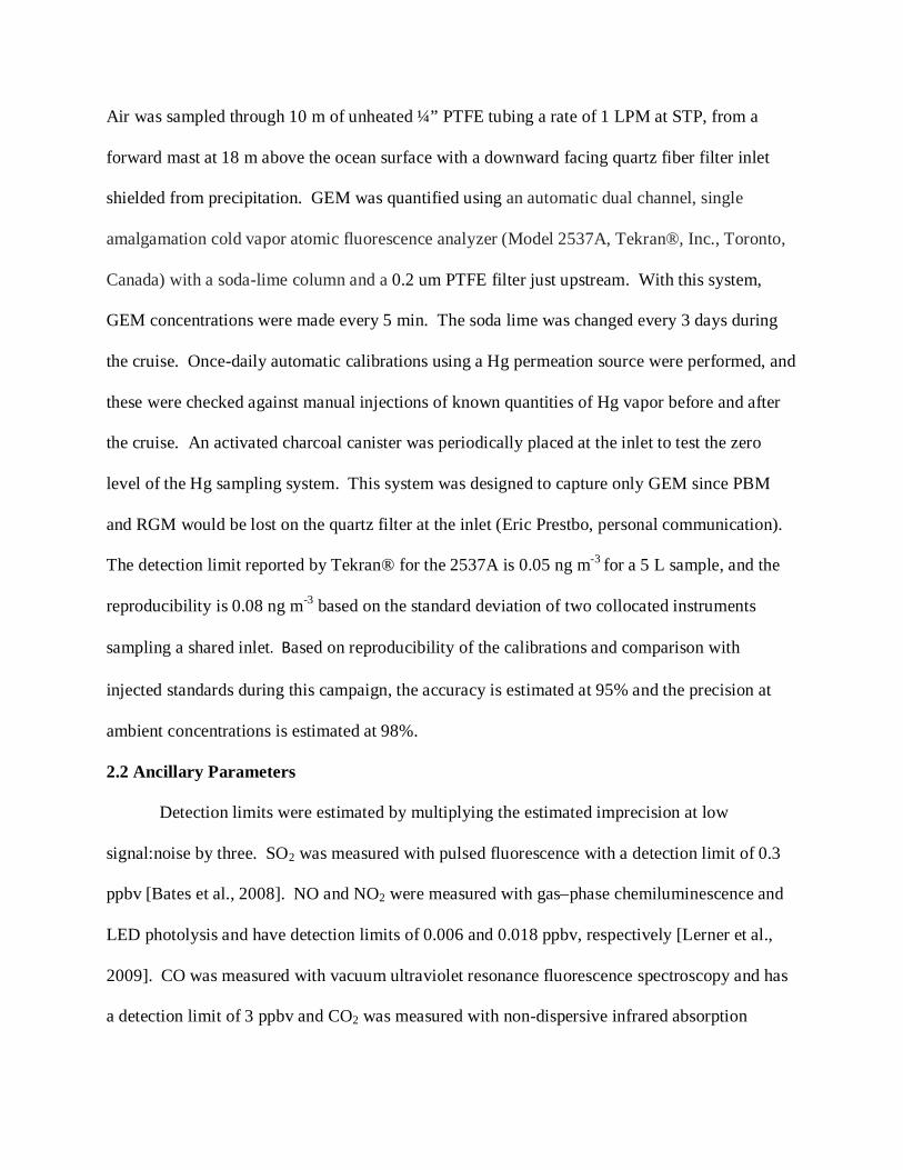
Air was sampled through 10 m of unheated ¼” PTFE tubing a rate of 1 LPM at STP, from a
forward mast at 18 m above the ocean surface with a downward facing quartz fiber filter inlet
shielded from precipitation. GEM was quantified using an automatic dual channel, single
amalgamation cold vapor atomic fluorescence analyzer (Model 2537A, Tekran®, Inc., Toronto,
Canada) with a soda-lime column and a 0.2 um PTFE filter just upstream. With this system,
GEM concentrations were made every 5 min. The soda lime was changed every 3 days during
the cruise. Once-daily automatic calibrations using a Hg permeation source were performed, and
these were checked against manual injections of known quantities of Hg vapor before and after
the cruise. An activated charcoal canister was periodically placed at the inlet to test the zero
level of the Hg sampling system. This system was designed to capture only GEM since PBM
and RGM would be lost on the quartz filter at the inlet (Eric Prestbo, personal communication).
The detection limit reported by Tekran® for the 2537A is 0.05 ng m-3 for a 5 L sample, and the
reproducibility is 0.08 ng m-3 based on the standard deviation of two collocated instruments
sampling a shared inlet. Based on reproducibility of the calibrations and comparison with
injected standards during this campaign, the accuracy is estimated at 95% and the precision at
ambient concentrations is estimated at 98%.
2.2 Ancillary Parameters
Detection limits were estimated by multiplying the estimated imprecision at low
signal:noise by three. SO2 was measured with pulsed fluorescence with a detection limit of 0.3
ppbv [Bates et al., 2008]. NO and NO2 were measured with gas–phase chemiluminescence and
LED photolysis and have detection limits of 0.006 and 0.018 ppbv, respectively [Lerner et al.,
2009]. CO was measured with vacuum ultraviolet resonance fluorescence spectroscopy and has
a detection limit of 3 ppbv and CO2 was measured with non-dispersive infrared absorption

spectroscopy and has a detection limit of 0.2 ppmv [Lerner et al., 2009]. Ozone was measured
using UV absorption with a detection limit of 3 ppbv [Williams et al., 2008]. An aerosol time-of
flight mass spectrometer (ATOFMS) measured real-time single particle size and composition;
data are shown with 5-min time resolution [Gard et al., 1997]. Seawater DMS was measured
using sulfur chemiluminescence with a detection limit of 0.6 nM [Bates et al., 2000]. Gas phase
dimethyl sulfide (DMS) was measured with a proton transfer reaction time of flight mass
spectrometer (PTR-TOF-MS) with a detection limit of 18 ppt for measurements at a 1-min time
resolution [Jordan et al., 2009].
Relative wind direction data were used to flag measurements when emissions from the
Atlantis may have been sampled, (relative wind > 75 degrees off the bow). Mean true wind
directions were determined by vector averaging. Statistical analyses were carried out using
Origin 7.5. Differences between population means were determined using a two sample t-test
and were considered significant if P < 0.05.
2.2 California Hg Emissions
Anthropogenic Hg emissions in California are a small contributor to global emissions
(approximately 1 Mg in 2010 or 0.05% of global emissions) [CARB, 2008; US EPA, 2012].
However about 40% of California’s point sources are located in the South Coast and Bay Area
Air Quality Districts, which include the areas around San Francisco and Los Angeles. Oil
refineries, waste incinerators, cement production and metal manufacturing facilities are the major
classes of industries that emit Hg in these metropolitan areas (Table 1). Gasoline and diesel
combustion by on-road mobile sources may make a minor contribution to atmospheric Hg based
on previous estimates [Conaway et al., 2005] but are not included in the CARB inventory.
Likewise, little is known about the Hg emissions from ocean-going ships, which may represent a

significant source of Hg in the vicinity of busy ports and shipping lanes [Sprovieri et al., 2010a].
Also uncertain is the speciation of Hg (i.e. GEM, RGM, and PBM) emitted from various industry
types. Hg emission estimates from 2008 for both the South Coast and Bay Area Air Quality
Districts are given in Table 1.
Estimates of emissions calculated with observed slopes between co-pollutants during
plume events are assumed to be valid as long as three assumptions are met: 1) no chemical or
physical loss of chemical species, only dilution, 2) constant emission source for each chemical
species with fixed ratios, and 3) constant background conditions of each chemical species [Jaffe
et al., 2005].
3. Results and Discussion
3.1 Overview of Cruise Segments
While the majority of the cruise was spent in Southern California (74% of time, latitude <
34.3 oN), the ship encountered many environments between San Diego and Sacramento, and was
likely influenced by varying emissions sources. Segments of the cruise were identified when the
ship was in a particular geographic location (e.g., Sacramento Ship Channel) and/or was likely
experiencing emissions of a distinct type, such as urban outflow, port industries, and ships at sea
[Ryerson et al., 2012]. GEM and other chemical species’ mean and maximum concentrations for
these segments are given in Table 2. In general the differences in mean GEM concentrations
between cruise segments were small (< 0.2 ng m-3). The segment with the highest mean GEM
concentration was the Port of Los Angeles (1.49 ng m-3), which was significantly higher than the
mean of all data and the means from other segments. The Port segment had the highest
maximum value for GEM (7.21 ng m-3) and also the highest maxima for CO, NO2, and SO2. The
highest mean CO and CO2 values were during the “outflow” conditions, when mobile sources

were likely more dominant, compared to the Port segment which had higher SO2 and NO mean
concentrations, and likely reflects a greater proportion of stationary source emissions in the Port
area. Outflow conditions also had significantly higher mean GEM concentrations compared to
the Southern California mean. Mean concentrations of CO2, CO, NO, NO2, and SO2 were
significantly higher from Southern California compared to means from the entire cruise, however
this was not the case for GEM, which had slightly higher concentrations (not significant) during
the whole cruise relative to Southern California. This suggests that in spite of the relatively
polluted conditions in Southern California, the GEM emissions in this region were relatively low
and did not greatly contribute to the Hg atmospheric burden. Likewise, GEM concentrations
were not greatly elevated in the San Francisco Bay and Carquinez Straits (maximum = 1.53 ng
m-3) where several oil refineries are located suggesting that GEM emissions in this region were
relatively low as well.
The open ocean and Monterey Bay sections of the cruise had the cleanest air quality
conditions, with NO+NO2 concentrations around 0.3 – 1.2 ppbv (compared to ~20 ppbv at the
Port). GEM was significantly lower during open ocean conditions compared to all the data,
suggesting the ocean source of GEM was not a strong contributor. Inland locations at West
Sacramento and in the Sacramento Ship Channel were also relatively unpolluted (NO+NO2 = 1.4
– 2.3 ppbv), which is consistent with these locations being rural. Mean GEM concentrations
were significantly higher in the West Sacramento region but not higher in the Ship Channel
compared to all the data suggesting multiple sources of GEM.
3.2 Diel Patterns in the South Coast Region
The sea/land breeze diel circulation within the Los Angeles Basin and adjacent waters
involves a relatively strong transport of air from the ocean into the basin during the day and a

weaker transport of urban air offshore during the night [Wagner et al., 2012]. Figure 2 shows
wind direction frequency, and median gaseous pollutant concentrations as a function of wind
direction, and Figure 3 shows the mean diel cycles for these parameters from all locations south
of 34.3 oN latitude. The coastline was generally to the north or northeast in this region, except in
Santa Monica Bay, where east and southeasterly directions also pointed toward land. The wind
observations here show a strong transport broadly consistent with a sea breeze, which occurred
between 14:00 – 20:00 local time, most frequently from the W and SW sectors (55% of time)
and was associated with the diel minima in GEM, CO2, CO and NO2. A weaker and shorter-lived
land breeze between 04:00 – 08:00 occurred with the diel maximum in GEM, CO2, CO and NO2.
GEM median concentrations were 1.33 ± 0.12 ng m-3 in the W sector compared to 1.45 ± 0.11 ng
m-3 in the NE sector, a similar dependence on wind direction as CO2, CO and to some extent
NO2. However the diel pattern of GEM displayed a later maximum at 09:00 – 11:00, compared
with the early morning maxima in CO2, CO, and NO2.
Median NO was strongly enhanced in the S, SW, and SE sectors indicating the directions
of nearest combustion sources in the Port area. Median SO2 was also enhanced in the S sector
along with the SE, E, and NE sectors. SO2 and NO displayed later diel maxima (10:00 – 14:00)
compared with CO2, CO, and NO2, The GEM diel maximum occurred between the diel maxima
of CO2, CO, and NO2, and the maxima of SO2 and NO. If the former group of pollutants
represents more aged emissions dominated by mobile and inland sources and the latter represents
fresh emissions dominated by point sources near the coast, the diel pattern of GEM suggests that
both types of sources contribute.
The diel cycle of “background” GEM (> 1.7 ng m-3 removed) is also shown in Figure 3.
Comparing these data with the diel cycle of all GEM data reveals that background GEM was

generally observed during the daytime and evening hours (12:00 – 22:00 local time) and most
GEM enhancements occurred during land breeze or transition periods (00:00 – 11:00).
Background GEM was most depleted relative to all GEM during the hours of 02:00 and 04:00
(difference of ~0.1 ng m-3), yet by 08:00 the difference between the means was only ~0.025 ng
m-3. This argues against significant loss of GEM via oxidation by Cl atoms which would be
identifiable by a post-sunrise dip in background GEM concentrations due to the production of Cl
atoms from ClNO2 photodecomposition at sunrise [Wagner et al., 2012, Riedel et al., 2012].
3.3 Los Angeles Port Emissions
The Los Angeles/Long Beach Port has some of the largest Hg emitting point sources in
southern California within about 10 km. The observed GEM:SO2 relationship during these
periods is shown in Figure 4A and the NOx:SO2 relationship is shown in Figure 4B, along with
the corresponding published ratios for each Hg-emitting facility in the area. Many of the GEM
concentrations during the Port segment were at or near background levels; out of 447 five-min
GEM data, only six observations were > 2 ng m-3 and 50 observations were > 1.7 ng m-3.
Nonetheless, the few enhanced GEM observations allow for a rough estimate of emission fluxes
from point sources in the area. The ratios of GEM enhancements vs. the co-pollutants CO, SO2,
and NOx in Plumes 1, 2 and 3 are given in Table 3, along with the 2008 emissions inventories for
some of the major local point sources. Plumes 1 and 2 occurred when the ship was stationary in
the upper Port area (denoted by the large magenta dot in Figure 1C) on two separate days,
5/20/10 (16:15 GMT) and 5/27/10 (16:50 GMT). The 5-min mean wind direction during these
two observations was 126 and 165 degrees, respectively. Plume 3 (smaller magenta dot in Figure
1C) occurred on 5/20/10 (18:45 GMT) in a location more to the SW, and was associated with a
wind direction of 42 degrees. From Figure 4A the reported GEM/SO2 from the SERRF facility
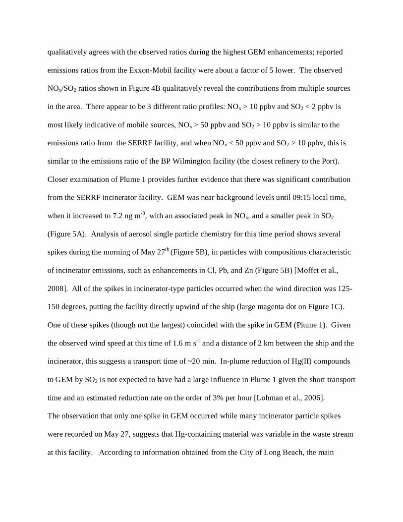
qualitatively agrees with the observed ratios during the highest GEM enhancements; reported
emissions ratios from the Exxon-Mobil facility were about a factor of 5 lower. The observed
NOx/SO2 ratios shown in Figure 4B qualitatively reveal the contributions from multiple sources
in the area. There appear to be 3 different ratio profiles: NOx > 10 ppbv and SO2 < 2 ppbv is
most likely indicative of mobile sources, NOx > 50 ppbv and SO2 > 10 ppbv is similar to the
emissions ratio from the SERRF facility, and when NOx < 50 ppbv and SO2 > 10 ppbv, this is
similar to the emissions ratio of the BP Wilmington facility (the closest refinery to the Port).
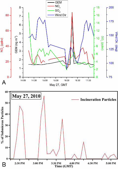
Closer examination of Plume 1 provides further evidence that there was significant contribution
from the SERRF incinerator facility. GEM was near background levels until 09:15 local time,
when it increased to 7.2 ng m-3, with an associated peak in NOx, and a smaller peak in SO2
(Figure 5A). Analysis of aerosol single particle chemistry for this time period shows several
spikes during the morning of May 27th (Figure 5B), in particles with compositions characteristic
of incinerator emissions, such as enhancements in Cl, Pb, and Zn (Figure 5B) [Moffet et al.,
2008]. All of the spikes in incinerator-type particles occurred when the wind direction was 125-
150 degrees, putting the facility directly upwind of the ship (large magenta dot on Figure 1C).
One of these spikes (though not the largest) coincided with the spike in GEM (Plume 1). Given
the observed wind speed at this time of 1.6 m s-1 and a distance of 2 km between the ship and the
incinerator, this suggests a transport time of ~20 min. In-plume reduction of Hg(II) compounds
to GEM by SO2 is not expected to have had a large influence in Plume 1 given the short transport
time and an estimated reduction rate on the order of 3% per hour [Lohman et al., 2006].
The observation that only one spike in GEM occurred while many incinerator particle spikes
were recorded on May 27, suggests that Hg-containing material was variable in the waste stream
at this facility. According to information obtained from the City of Long Beach, the main

sources of Hg in the waste stream would have been electronic and household hazardous waste.
Beginning in the spring of 2010 aggressive efforts were taken to divert these items from the
waste stream and subsequent emissions of Hg from the SERRF incinerator in 2011 decreased to
~2% of the value reported in the 2008 CARB inventory. However, our results here suggest that
during May 2010 when the GEM spike was observed, full Hg waste reductions had not yet
occurred and emissions were closer to the 2008 levels.
3.4 Los Angeles Urban Outflow
Los Angeles urban outflow conditions typically occurred at night or the early morning
when winds tended to be from the northern or eastern sectors (Figures 2 and 3). The highest
GEM enhancements under these conditions were when the ship was located in the Santa Monica
Bay, (Figure 1B) (max GEM = 1.70 ng m-3, Table 1). These time periods reveal different
chemical profiles compared to what was observed in the Port segments. NOx vs. SO2 in Figure
6B shows two distinct sources of polluted air, consistent with mobile emissions (NOx > 10 ppbv,
SO2 < 1.5 ppbv) and refinery emissions (NOx < 15 ppbv, SO2 > 1 ppbv). GEM concentrations in
the suspected refinery plumes (Figure 6A) were less than those predicted based on the 2008
GEM inventory for the Chevron facility located on Santa Monica Bay at El Segundo, suggesting
that refinery emissions were lower in 2010 than 2008. GEM was not correlated with SO2 in
outflow conditions (R2 = 0), but GEM and CO were positively correlated (Figure 6C) producing
a slope of 0.0011 ng m-3 ppbv-1, which corresponds to 1.23 x 10⁻⁷ mol mol-1. In comparison,
outflow from China, which was sampled in Okinawa, Japan produced a mean total Hg:CO ratio
of 6.2 x 10⁻⁷ mol mol-1 [Jaffe et al., 2005] ,a factor of five larger than our measurements during
CalNex. The lack of coal combustion in the Southern California may be one reason why the
observed ratio is lower compared to that from downwind of Asian sources.

Assuming that 3.85 x 10¹⁰ mol of CO were released annually in the South Coast Air
Quality District (SCAQD) [CARB, 2008], and using the observed GEM/CO ratio in Outflow
conditions, GEM emissions can be roughly estimated at 1500 kg annually. This value is a factor
of 20 larger than the GEM point source emissions from the SCAQD (Table 1). Since CO
emissions in Los Angeles are dominated by mobile sources, the question arises whether these
could be contributing to GEM enhancements. Previous tests on gasoline in the San Francisco
Bay Area showed that the average Hg content was 0.5 ng g-1 [Conaway et al., 2005]. Assuming
32 x 109 liters of gasoline were consumed in Imperial, Los Angeles, Orange, Riverside, San
Bernardino, and Ventura counties during 2008 [Caltrans, 2012], this suggests that approximately
12 kg of Hg could be emitted annually from automobiles across these six counties, which is a
minor contributor. Another contributing source could be reemission of GEM from land and
vegetation surfaces from the cumulative deposition of anthropogenic Hg over time. While data
on this are sparse, models suggest that reemission is important globally, contributing 3 times the
emissions from primary anthropogenic sources [Selin et al., 2007].
3.5 Ship Emissions
The R/V Atlantis sampled the exhaust of many large ships in and around the Port of Los
Angeles, during CalNex. One such encounter, which lasted almost 50 minutes, was with a cargo
ship, the M/V Margrethe Maersk [Lack et al., 2011], in which NOx concentrations increased
from near zero outside the plume to almost 100 ppbv within the plume. CO2 and GEM
concentrations and CO2 and NOx concentrations were positively correlated (Figure 7). The slope
of the linear relationship between GEM and CO2 for this plume is 0.031 ng m-3 ppmv-1, which
converts to 3.5 x 10⁻⁹ mol mol-1. Assuming 3170 g CO2 per kg of fuel burned [Williams et al.,
2009], and using the observed GEM:CO2 ratio, gives a mass-based emissions factor of 0.05 ±

0.01 mg GEM per kg fuel burned. This corresponds to roughly 14 Mg y-1 of Hg for global
shipping, which is a minor contributor globally (< 1% global anthropogenic sources), but may be
an important source locally in ports.
Limited data on marine fuels suggests that the Hg content of both distillate and residual
marine fuels spans two orders of magnitude (0.001 to 0.1 mg kg-1) [Lloyd’s, 1995]. Without the
Hg content in the fuel that was being burned during the plume encounter, it is difficult to assess
the effects of combustion and emission control on Hg content in the plume. Furthermore,
significant amounts of HgII and particulate Hg could be emitted in ship exhaust and these species
were not measured here. More data are needed on Hg in ship plumes in order to verify the large
range in Hg content in fuels and to determine if there are differences in Hg emissions factors
between ships burning residual vs. distillate fuels.
3.6 San Francisco Bay and Carquinez Straits Emissions
GEM concentrations in the industrial and urban regions of the San Francisco Bay and the
Carquinez Straits (maximum GEM = 1.53 ng m-3) were not nearly as high compared to GEM
concentrations in the Port of Los Angeles or in Los Angeles urban outflow. Figure 1D shows the
GEM concentrations measured, the locations of oil refineries, and the locations of the highest
SO2 observations (~9 ppbv). Figure 8A shows the GEM:SO2 relationship and Figure 8B shows
the NOx:SO2 relationship in this region. For comparison, the mean reported total Hg:SO2 and
NOx:SO2 ratios from 2008 CARB inventory for the local refineries are also shown. Similar to
the Los Angeles Outflow, Figure 8B shows a cluster of points associated with high
SO2/moderate NOx that is captured within the range of emissions ratios reported for the local
refineries. The cluster of data points with SO2 < 1 ppbv and NOx > 5 ppbv are characteristic of
mobile source emissions. As shown in Figure 8A, however, GEM was only slightly enhanced

during high SO2 periods, and produced an observed GEM/SO2 ratio that matched output from the
Shell and Valero facilities. Note that the highest SO2 observations corresponded to when the
ship was in a part of the Carquinez Straits that was closer to the Shell and Valero, compared to
the Conoco-Phillips facilities, so these results are consistent.
3.7 GEM Emissions from Coastal Waters
Photolytic processes are generally the main driver of Hg2+ reduction to Hg0 in surface
waters, although biotic reduction can also occur [Pirrone et al., 2010; Sorenson et al., 2010]. Hg0
has generally been observed to be supersaturated with respect to atmospheric concentrations in
most oceanic locations. As a result, the global oceans represent a large emission source of GEM,
on par with the magnitude of the anthropogenic source [Pirrone et al., 2010], but the estimates
are very uncertain. A review of measurements of the GEM ocean-air flux determined by
dissolved gaseous Hg concentrations and gas exchange models shows a wide range of values,
from 1 x 10⁻⁴ to 0.01 µmol m-2 d-1 [Sprovieri et al., 2010b]. Coastal and inland seas typically
have the highest evasional fluxes [Pirrone et al., 2010] .
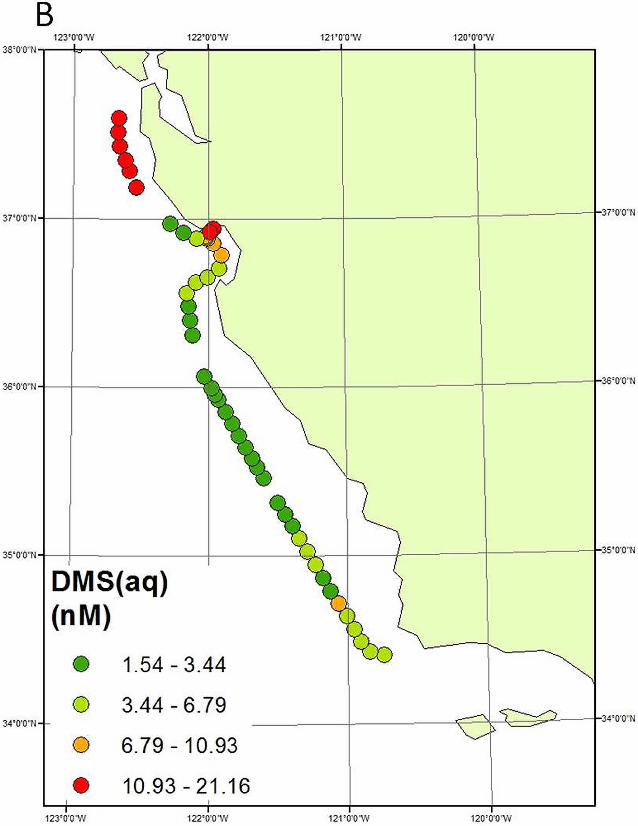
This cruise afforded an opportunity to assess the GEM emissions from coastal waters
where upwelling could result in higher GEM evasion rates through an increased Hg(II) flux into
the mixed layer. On June 2, 2010 near noon local time the ship was offshore of Pt. Ano Nuevo,
an area known for strong upwelling [Ryan et al., 2010]. Here, an atmospheric GEM
enhancement of ~0.3 ng m-3 was observed, that was sustained for ~5 hours over ~60 km (Figure
9). During this period GEM concentrations were uncorrelated with CO (R2 = 0.01), but were
weakly positively correlated with wind speed (R2 = 0.19,) sea surface temperature (R2 = 0.54),
and chlorophyll (R2 = 0.07). GEM was negatively correlated with salinity (R2 = 0.20). GEM
was also positively correlated with DMS in seawater (R2 = 0.28) and DMS in the atmosphere (R2

= 0.16). As DMS is an indicator of oxidative stress and cell lysis in marine phytoplankton
[Wolfe and Steinke, 1996], the correlation of GEM with DMS suggests that the GEM observed
here is related to phytoplankton cell lysis. The correlations of GEM with SST and salinity
suggest that as the water moves away from the upwelled region, which is relatively cold and
saline, it warms and the phytoplankton die (or get consumed). GEM and DMSP (DMS
precursor) are then released to the water column creating supersaturation and a net evasional flux
which is also dependent on wind speed.
The slope of the GEM:DMS(g) relationship was 0.0089 ± 0.005 ng m-3 pptv, which
converts to 9.9 x 10⁻⁴ mol GEM mol-1 DMS. The calculated DMS ocean to atmosphere flux in
this region, based on seawater DMS concentrations, wind speed and sea surface temperature
ranged from 8 to 39 µmol m-2 d-1 (mean 17 ± 9.5 µmol m-2 d-1). Based on the GEM:DMS(g)
relationship, the corresponding GEM flux for this region was 0.017 ± 0.009 µmol m-2 d-1. This
value is on the upper end of the measurements reported in Sprovieri et al. [2010b]. To determine
if Hg0 subsurface concentrations could sustain such a high evasion rate we estimated that given
an open ocean concentration of 1 pM Hg0 in the mixed layer [Mason and Sullivan, 1999], the
observed flux would ventilate all of the Hg0 in a 50 m mixed layer in ~2 days. This would likely
outstrip the inventory of Hg0 even with upwelling. Thus, for the observed flux to be plausible,
there must be a fast conversion of Hg(II) to Hg0. If Hg(II) is around 2 pM in the mixed layer
[Mason and Sullivan, 1999], then the reduction rate would have to be around 10% per day to
sustain the observed flux. This is an order of magnitude higher than what is thought to be the
Hg0 formation rate in the equatorial Pacific [Mason et al., 1994]. Thus, as not a lot is known
about Hg in upwelling regions, more data are needed to constrain the concentrations of Hg
species, and compare the expected flux with that observed here.

4. Conclusions
These data contribute to the understanding of the various anthropogenic and natural
sources of GEM in the atmosphere of coastal California. Overall, most GEM concentrations
were representative of background conditions. The mean GEM concentration from southern
California (< 34.3 oN), near most of the anthropogenic sources, was not higher than the mean
concentration for the entire cruise. However, certain periods were identified when the air
sampled was likely influenced by Port of Long Beach emissions, Los Angeles urban outflow,
cargo ships, Carquinez Straits emissions, and natural oceanic emissions. GEM enhancements
were observed during all these events and estimates of the GEM flux from these sources were
made. In the Port of Long Beach, GEM was enhanced up to 7 ng m-3 on three occasions, and
observed GEM/SO2 and NOx/SO2 ratios were consistent with the 2008 Hg, SO2, and NO2
inventories for the incinerator facility. Furthermore, single particle composition during the
largest event showed enhancements in the elements characteristic of incinerator emissions.
The Los Angeles urban outflow was observed generally at night and in the early morning,
when CO, CO2, and NO2 displayed their diel maxima. GEM and CO concentrations were
positively correlated with a slope of 0.0011 ng m-3 ppbv-1 (1.23 x 10⁻⁷ mol mol-1) during these
periods, which given the inventoried CO emissions for the region, suggests a larger source of
GEM than is accounted for by the inventory. Reemissions of previously deposited mercury may
be contributing to this discrepancy.
The diel maximum in GEM concentrations for all data from < 34.3 oN occurred in the
mid morning (8:00 – 12:00 local time), which was intermediate between the diel maxima of CO
and CO2, and the diel maxima of NO and SO2. This suggests that there are two types of sources
of GEM from the urban area, one associated with point sources in the Port (higher NO and SO2)

and another associated with sources located further away from the coast (higher CO and CO2).
There was no observable post-sunrise dip in GEM concentrations during relatively unpolluted
conditions, which suggests that reaction of GEM with atomic chlorine was probably not a large
sink for GEM.
A plume from a large cargo ship was observed with a positive correlation between
GEM:CO2, and GEM:NOx. Using conversions for g CO2 per kg of fuel burned, an estimate of a
mass-based emissions factor of 0.05 ± 0.01 mg GEM per kg fuel burned for this particular plume
was obtained. This corresponds to roughly 14 Mg y-1 of Hg for global shipping, which is a
minor contributor globally (< 1% global anthropogenic sources), but may be an important source
locally in ports. These estimates are limited by lack of knowledge of the Hg content in the
unburned fuel and Hg speciation in the atmosphere.
GEM concentrations in the Carquinez Straits where many large oil refineries are located
were rarely significantly elevated above the background. In an area where observed NOx:SO2
ratios indicated impacts from local oil refineries, the observed GEM concentrations were less
than those predicted based on the 2008 emissions inventories for these facilities, indicating that
GEM emission may have been reduced.
In a roughly 60 km part of the cruise track, in between Monterey Bay and the Golden
Gate, GEM was enhanced and positively correlated with DMS in seawater and the atmosphere.
This suggests an oceanic source of GEM. The measured DMS flux in this region was 17 ± 9.5
µmol m-2 d-1, which implies a GEM flux of 0.017 ± 0.009 µmol m-2 d-1. This flux is on the high
end of what has been observed in other locations and more data are needed to understand the
potential for extremely high GEM fluxes in regions affected by coastal upwelling.

Acknowledgements. We thank the captain and crew of the R/V WHOI Atlantis, Patricia Quinn
of NOAA-PMEL, Andrew Lincoff of EPA Region 9, and Lucas Hawkins and Eric Prestbo of
Tekran Inc.
References Ariya, P. A., A. Khalizov, and A. Gidas (2002) Reactions of gaseous mercury with atomic and molecular halogens: kinetics, product studies, and atmospheric implications, J. Phys. Chem. A, 106, 7310-7320. Bates, T. S., P. K. Quinn, D. S. Covert, D. J. Coffman, J. E. Johnson, and A. Wiedensohler. (2000), Aerosol physical properties and controlling processes in the lower marine boundary layer: A comparison of submicron data from ACE-1 and ACE-2. Tellus, 52B, 258 – 272. Bates, T. S., et al. (2008), Boundary layer aerosol chemistry during TexAQS/GoMACCS 2006: Insights into aerosol sources and transformation processes, J. Geophys. Res., 113, D00F01, doi:10.1029/2008JD010023. Beldowska, M., D. Saniewska, L. Falkowska, and A. Lewandowska (2012), Mercury in particulate matter over Polish zone of the southern Baltic Sea, Atmos. Environ. 46, 397-404. California Air Resources Board, 2008 Emissions Inventory, available online at http://www.arb.ca.gov. Caltrans, California Department of Transportation, http://www.dot.ca.gov/dist12/, accessed 10/10/2012. Conaway, C. H., R. P. Mason, D. J. Steding, A. R. Flegal (2005), Estimate of mercury emission from gasoline and diesel fuel consumption, San Francisco Bay area, California, Atmos. Environ. 39, 101–105. Dastoor, A., and Larocque, Y.: Global circulation of atmospheric mercury: a modelling study, Atmos. Environ., 38, 147-161, 2004. Fitzgerald, W. F., C. H. Lamborg, and C. R. Hammerschmidt, (2007), Marine biogeochemical cycling of mercury, Chem. Rev., 107, 641-662. Gard, E., J. E. Mayer, B. D. Morrical, T. Dienes, D. P. Fergenson, and K. A. Prather (1997), Real-time analysis of individual atmospheric aerosol particles: Design and performance of a portable ATOFMS, Anal. Chem., 69(20), 4083–4091, doi:10.1021/ac970540n. Jaffe, D., E. Prestbo, P. Swartzendruber, P. Weiss-Penzias, S. Kato, A. Takami, S. Hatakeyama, and Y. Kajii (2005), Export of atmospheric mercury from Asia. Atmos. Environ. 39, 3029– 3038.

Jordan A., S. Haidacher, G. Hanel, E. Hartungen, L. Mark, H. Seehauser, R. Schottkowsky, P. Sulzer, and T. D. Mark (2009), A high resolution and high sensitivity proton-transfer-reaction time-of-flight mass spectrometer (PTR-TOF-MS), Intl J. Mass Spectrometery, 286, 122-128, doi:620 10.1016/j.ijms.2009.07.005. Holmes, C. D., D. J. Jacob, E. S. Corbitt, J. Mao, X. Yang, R. Talbot, and F. Slemr (2010), Global atmospheric model for mercury including oxidation by bromine atoms, Atmos. Chem. Phys., 10, 12037-12057. Lack, D. A., et al. (2011) Impact of fuel quality regulation and speed reductions on shipping emissions: implications for climate and air quality, Environ. Sci. Technol., 45, 9052–9060, doi.org/10.1021/es2013424. Lerner, B. M., P. C. Murphy, and E. J. Williams (2009), Field measurements of small marine craft gaseous emission factors during NEAQS 2004 and TexAQS 2006, Environ. Sci. Technol., 43, 8213-8219, doi: 10.1021/es901191p. Lindberg, S., R. Bullock, R. Ebinghaus, D. Engstrom, X. Feng, W. Fitzgerald, N. Pirrone, E. Prestbo, and C. Seigneur (2007), Synthesis of Progress and Uncertainties in Attributing the Sources of Mercury in Deposition, Ambio, 36, 19-33. Lloyd’s Register Engineering Services (1995), Marine Exhaust Emissions Research Programme, London. Lohman, K., C. Seigneur, E. Edgerton and J. Jansen (2006), Modeling mercury in power plant plumes, Environ. Sci.Technol., 40, 3848-3854. Mahaffey, K. R., R. P. Clickner, and C.C. Bodurow (2004), Blood organic mercury and dietary mercury intake: National Health and Nutrition Examination Survey, 1999 and 2000. Environ. Health Perspect. 112, 562–70. Malcolm, E. G., A. C. Ford, T. A. Redding, M. C. Richardson, B. M. Strain, and S. W. Tetzner (2009), Experimental investigation of the scavenging of gaseous mercury by sea salt aerosol, J. Atmos. Chem., 63, 221-234. Mason, R. P., W. F. Fitzgerald, and F. M. M Morel (1994), The biogeochemical cycling of elemental mercury: anthropogenic influences, Geochim. Cosmochim. Acta, 58, 3191-3198. Mason, R. P., and K. A. Sullivan (1999), The distribution and speciation of mercury in the South and equatorial Atlantic, Deep Sea Res. II, 46, 937-956. Mason, R. P., and G.-R. Sheu (2002), Role of the ocean in the global mercury cycle, Global Biogeochem. Cycles, 16, 1093,10.1029/2001GB001440. Mergler, D., H. A. Anderson, L. H. M. Chan, K. R. Mahaffey, M. Murray, M. Sakamoto and A. H. Stern (2008), Methylmercury exposure and health effects in humans: a worldwide concern, Ambio, 36, 3-11.

Moffet, R. C., Y. Desyaterik, R. J. Hopkins, A. V. Tivanski, M. K. Gilles, Y. Wang, V. Shutthanandan, L. T. Molina, R. G. Abraham, K. S. Johnson, V. Mugica, M. J. Molina, A. Laskin, and K. Prather (2008), Characterization of aerosols containing Zn, Pb, and Cl from an industrial region of Mexico City, Environ. Sci. Technol., 42, 7091–7097. Pirrone, N., S. Cinnirella, X. Feng, R. B. Finkelman, H. R. Friedli, J. Leaner, R. Mason, A. B. Mukherjee, G. B. Stracher, D. G. Streets, and K. Telmer (2010), Global mercury emissions to the atmosphere from anthropogenic and natural sources, Atmos. Chem. Phys., 10, 5951–5964, 2010. Riedel, T. P., T. H. Bertram, T. A. Crisp, E. J. Williams, B. M. Lerner, A. Vlasenko, S-M. Li, J. Gilman, J. de Gouw, D. M. Bon, N. L. Wagner, S. S. Brown, and J. A. Thornton (2012) Nitryl chloride and molecular chlorine in the coastal marine boundary layer, Environ. Sci. Technol.,
dx.doi.org/10.1021/es204632r. Ryan J. P., S. B. Johnson, A. Sherman, K. Rajan, F. Py, H. Thomas, J. B. J. Harvey, L. Bird, J. D. Paduan, and R. C. Vrijenhoek (2010), Mobile autonomous process sampling within coastal ocean observing systems, Limnol. Oceanogr.: Methods, 8, 394–402. T.B. Ryerson, A.E. Andrews, W.M. Angevine, T.S. Bates, C.A. Brock, B. Cairns, R.C. Cohen, O.R. Cooper, J.A. de Gouw, F.C. Fehsenfeld, R.A. Ferrare, M.L. Fischer, R.C. Flagan, A.H. Goldstein, J.W. Hair, R.M. Hardesty, C.A. Hostetler, J.L. Jimenez, A.O. Langford, E. McCauley, S.A. McKeen, L.T. Molina, A. Nenes, S.J. Oltmans, D.D. Parrish, J.R. Pederson, R.B. Pierce, K. Prather, P.K. Quinn, J.H. Seinfeld, C.J. Senff, A. Sorooshian, J. Stutz, J.D. Surratt, M. Trainer, R. Volkamer, E.J. Williams, and S.C. Wofsy (2012), The 2010 California research at the nexus of air quality and climate change (CalNex) field study, submitted to J. Geophys. Res. Selin, N. E., D. J. Jacob, R. J. Park, R. M. Yantosca, S. Strode, L. Jaeglé, and D. Jaffe (2007), Chemical cycling and deposition of atmospheric mercury: Global constraints from observations, J. Geophys. Res., 112, D02308, doi:10.1029/2006JD007450. Shia, R. L., Seigneur, C., Pai, P., Ko, M., and Sze, N. D. (1999) Global simulation of atmospheric mercury concentrations and deposition fluxes, J. Geophys. Res., 104, 23747-23760. Soerensen, A. L., E. M. Sunderland, C. D. Holmes, D. J. Jacob, R. M. Yantosca, H. Skov, J. H. Christensen, S. A. Strode, and R. P. Mason (2010), An improved global model for air-sea exchange of mercury: high concentrations over the North Atlantic, Environ. Sci. Technol., 44, 8574-8580. Snyder, D. C., T. R. Dallmann, J. J. Schauer, T. Holloway, M. J. Kleeman, M. D. Geller, and C Sioutas (2008), Direct observation of the break-up of a nocturnal inversion layer using elemental mercury as a tracer, Geophys. Res. Lett., 35, L17812, doi:10.1029/2008GL034840. Sprovieri, F., I. M. Hedgecock, and N. Pirrone (2010a), An investigation of the origins of reactive gaseous mercury in the Mediterranean marine boundary layer, Atmos. Chem. Phys., 10, 3985–3997.

Sprovieri, F., N. Pirrone, R. Ebinghaus, H. Kock, and A. Dommergue (2010b), A review of worldwide atmospheric mercury measurements, Atmos. Chem. Phys., 10, 8245–8265. US EPA “Estimated per capita fish consumption in the United States, August 2002” (2002a), United States Environmental Protection Agency. US EPA, National Emissions Inventory for 2002 (2002b), United States Environmental Protection Agency. US EPA “Toxics Release Inventory” (2012), available online at: http://www.epa.gov/tri Wagner N. L., T. P. Riedel, J. M. Roberts, J. A. Thornton, W. M. Angevine, E. J. Williams, B. M. Lerner, A. Vlasenko, S. M. Li, W. P. Dubé, D. J. Coffman, D. M. Bon, J. A. de Gouw, W. C. Kuster, J. B. Gilman, S. S. Brown, The sea breeze / land breeze circulation in Los Angeles and its influence on nitryl chloride production in this region, Submitted to J. Geophys. Res. 2012. Williams, E. J., F. C. Fehsenfeld, B. T. Jobson, W. C. Kuster, P. D. Goldan, J. Stutx and W. A. McClenny (2008), Comparison of ultraviolet absorbance, chemiluminescence, and DOAS instruments for ambient ozone monitoring, Environ. Sci. Technol., 40, 5755-5762, doi: 10.1021/es0523542. Williams, E. J., B. M. Lerner, P. C. Murphy, S. C. Herndon, and M. S. Zahniser (2009), Emissions of NOx, SO2, CO, and HCHO from commercial marine shipping during Texas Air Quality Study (TexAQS) 2006, J. Geophys. Res., 114, D21306, doi:10.1029/2009JD012094. Wolfe, G. V., and M. Steinke (1996), Grazing-activated production of dimethyl sulfide (DMS) by two clones of Emiliania huxleyi, Limnol. Oceanogr., 41, 1151-1160. Zhang, Y., L. Jaegle’, A. van Donkelaar, R. V. Martin2, C. D. Holmes, H. M. Amos4, Q. Wang, R. Talbot, R. Artz, S. Brooks, W. Luke, T. M. Holsen, D. Felton, E. K. Miller, K. D. Perry, D. Schmeltz, A. Steffen, R. Tordon, P. Weiss-Penzias, and R. Zsolway (2012), Nested-grid simulation of mercury over North America, Atmos. Chem. Phys. Discuss., 12, 2603–2646.

Figure Captions:
Figure 1: Cruise track of the R/V Atlantis between San Diego and San Francisco, California, May 14 – June 8, 2012 with 5-min GEM concentrations and known GEM point source emissions. A) Entire cruise track, B) Southern California, C) Port of Los Angeles, and D) San Francisco Bay and Carquinez Straits. Magenta dots in (C) and (D) indicate the ship’s position during plume encounters detailed in Figs. 4 and 8, respectively.
Figure 2: Wind direction frequency and median concentrations of chemical species by 45 degree wind direction bins for all 5-min data from Southern California (south of 34.3 oN).
Figure 3: Diel bin plots for CO2, CO, wind direction, O3, GEM, NOx, SO2 and wind speed for Southern California 5-min data. GEM background is a subset of data with 5-min GEM > 1.7 ng m-3 removed.
Figure 4: A) GEM and B) NOx 5-min measurements plotted against 5-min SO2 data during periods when the ship was in the Port of Los Angeles. Lines show the mean reported total Hg:SO2 and NOx:SO2 ratios from 2008 CARB inventory for the point sources listed. An offset of 1.3 ng m-3 GEM and 10 ppbv NOx was added to the inventory ratios in plots A and B, respectively.
Figure 5: Close up of LA Port event with the highest GEM observation. A) GEM, NOx, SO2, and wind direction. B) Aerosol time-of-flight mass spectrometer (ATOFMS) results for percent of submicron particles with compositions representative of incineration particles.
Figure 6: Scatter plots with linear fits of A) GEM vs. SO2, B) NOx vs. SO2, and GEM vs. CO during times classified as Los Angeles outflow.
Figure 7: GEM vs. CO2 and NOx vs. CO2 during a 50 minute period on May 25, 2010 when an exhaust plume from a cargo ship the Margarethe Maersk was encountered.
Figure 8: A) GEM and B) NOx 5-min measurements plotted against 5-min SO2 data during periods when the ship was passing through San Francisco Bay and the Carquinez Strait. Lines show the mean reported total Hg:SO2 and NOx:SO2 ratios from 2008 CARB inventory for the various point sources listed. An 1.3 ng m-3 was added as an offset to the refinery GEM:SO2 ratios in plot A.
Figure 9: Comparison of spatial patterns of atmospheric GEM with seawater DMS (A and B) during the open ocean portion of the cruise (30 min data are shown). Panels C and D show the relationships between 30-min GEM and seawater DMS and atmospheric DMS for the data from the circled regions.

Table 1: Major Hg Emitters in San Francisco and Los Angeles Areas1
Name City Total Hg
Emissions kg y-1 Estimated % GEM of
total Hg emitted2
Lehigh Southwest Cement Cupertino 81.3 75 Conoco Phillips Refinery (1) Rodeo 79.5 80
Conoco Phillips Refinery (2) Rodeo 35.1 80
Valero Refinery Benicia 14.2 80
Bubbling Well Pet Memorial Fairfield 3.0 20-50
Shell Refinery Martinez 3.0 80
ALL SOURCES Bay Area Air Quality
District 240.0
Exxon-Mobil Refinery Torrance 73.1 80
SE Resourcs Recovery (SERRF) Incinerator Long Beach 60.3 22
Quemetco Metals Processing City of Industry 10.1 80
Chevron Refinery El Segundo 7.1 80
BP West Coast Refinery Carson 7.0 80
ALL SOURCES South Coast Air Quality
District 170.0
12008 California Air Resources Board Inventory
2Hg speciation data taken from 2002 National Emissions Inventory, which has fixed ratios for each emitting type.

Table 2: Chemical concentrations by cruise segment.1
Mean (Maximum) Concentrations
N GEM (ng m-3) CO2 (ppmv) CO (ppbv) NO (ppbv) NO2 (ppbv) SO2 (ppbv)
Outflow 570 1.41 (1.72) 405.2 (422.6) 182.8 (335.3) 0.71 (10.8) 6.39 (34.7) 0.44 (3.5)
Ships 146 1.31 (1.38) 395.3 (400.1) 132.4 (160.4) 2.41 (60.0) 3.17 (38.1) 0.23 (2.2)
Port 447 1.49 (7.21) 403.2 (429.9) 171.0 (443.0) 7.76 (130) 11.49 (43.7) 2.83 (25.1)
Open Ocean 355 1.37 (1.56) 394.1 (397.3) 112.1 (121.8) 0.10 (9.4) 0.22 (11.1) 0.01 (0.7)
Mont. Bay 156 1.32 (1.46) 401.7 (439.5) 121.2 (127.1) 0.09 (1.4) 1.14 (10.9) 0.03 (0.1)
SFBay/Carquinez 358 1.41 (1.53) 400.9 (413.8) 121.4 (171.5) 0.64 (17.2) 3.31 (10.7) 0.63 (9.4)
Sac. Ship Channel 129 1.40 (1.70) 393.4 (403.0) 111.2 (137.6) 0.33 (3.0) 0.97 (5.0) 0.36 (3.1)
W. Sacramento 458 1.45 (1.65) 401.8 (414.9) 108.0 137.9) 0.37 (8.1) 1.91 (7.4) 0.23 (1.0)
All Southern CA 4608 1.38 (7.21) 401.2 (433.1) 158.5 (443.0) 2.42 (130) 5.71 (43.7) 0.90 (25.1)
All Cruise 6789 1.41 (7.21) 400.0 (439.5) 139.1 (443.0) 1.86 (194) 3.91 (43.7) 0.61 (25.1)
1Cruise segments determined by analysis of ancillary parameters such as wind direction, CO2, and CO concentrations. Southern CA defined as all locations south of 34.3 oN latitude. N refers to 5-min GEM measurements.

Table 3: Ratios between pollutant concentrations during the 3 largest GEM plumes observed in the Los Angeles/Long Beach Port area compared with emissions ratios from nearby facilities from the 2008 CARB inventory.
GEM/CO1
ng m-3 ppb-1 GEM/SO2
ng m-3 ppb-1 GEM/NOx
ng m-3 ppb-1 NOx/SO2
ng m-3 ppb-1 Observation
Plume 1 0.10 1.14 0.07 16.0 Plume 2 0.21 5.91 0.24 24.4 Plume 3 0.07 1.53 0.10 15.8
Plume mean ± sd 0.13 ± 0.06 2.9 ± 2.2 0.14 ± 0.08 18.7 ± 4.0
Emissions Inventory
SERRF2 0.87 2.19 0.52 4.2 Exxon-Mobil 0.09 0.70 0.22 3.2
Chevron 0.01 0.05 0.02 2.8 BP Carson 0.02 0.02 0.02 1.1
1Calculated as (GEMplume – GEMbackground) / (COplume – CObackground). Background values used were GEM: 1.3 ng m-3, CO: 132 ppbv, SO2: 0.1 ppbv, NOx: 1 ppbv.
2SERRF emissions have been combined with the Quemetco emission from Table 1 (same location).