sheldon spectrum and the plankton paradox: two sides of ... · coexistence of a continuum of...

J. Math. Biol. (2018) 76:67–96https://doi.org/10.1007/s00285-017-1132-7 Mathematical Biology

Sheldon spectrum and the plankton paradox: two sidesof the same coin—a trait-based plankton size-spectrummodel

José A. Cuesta1,2 · Gustav W. Delius3 ·Richard Law3

Received: 20 July 2016 / Revised: 18 April 2017 / Published online: 25 May 2017© The Author(s) 2017. This article is an open access publication

Abstract The Sheldon spectrum describes a remarkable regularity in aquatic ecosys-tems: the biomass density as a function of logarithmic body mass is approximatelyconstant over many orders of magnitude. While size-spectrum models have explainedthis phenomenon for assemblages of multicellular organisms, this paper introducesa species-resolved size-spectrum model to explain the phenomenon in unicellularplankton. A Sheldon spectrum spanning the cell-size range of unicellular planktonnecessarily consists of a large number of coexisting species covering a wide range ofcharacteristic sizes. The coexistence ofmany phytoplankton species feeding on a smallnumber of resources is known as the Paradox of the Plankton. Our model resolves theparadox by showing that coexistence is facilitated by the allometric scaling of fourphysiological rates. Two of the allometries have empirical support, the remaining twoemerge frompredator–prey interactions exactlywhen the abundances follow aSheldon

B Gustav W. [email protected]://www.york.ac.uk/maths/staff/gustav-delius/

José A. [email protected]://gisc.uc3m.es/∼cuesta/

Richard [email protected]://www.york.ac.uk/maths/staff/richard-law/

1 Grupo Interdisciplinar de Sistemas Complejos (GISC), UC3M-BS Institute of Financial Big Data(IFiBiD), Departamento de Matemáticas, Universidad Carlos III de Madrid, Madrid, Spain

2 Instituto de Biocomputación y Física de Sistemas Complejos (BIFI), Universidad de Zaragoza,Zaragoza, Spain

3 Department of Mathematics and the York Centre for Complex Systems Analysis, University ofYork, York, UK

123

http://crossmark.crossref.org/dialog/?doi=10.1007/s00285-017-1132-7&domain=pdf

http://orcid.org/0000-0001-9482-2336

http://orcid.org/0000-0003-4092-8228

68 J. A. Cuesta et al.

spectrum. Our plankton model is a scale-invariant trait-based size-spectrum model:it describes the abundance of phyto- and zooplankton cells as a function of both sizeand species trait (the maximal size before cell division). It incorporates growth dueto resource consumption and predation on smaller cells, death due to predation, anda flexible cell division process. We give analytic solutions at steady state for both thewithin-species size distributions and the relative abundances across species.

Keywords Plankton · Coexistence · Allometry · Size-spectrum · Scale-invariance ·Cell division

Mathematics Subject Classification 92D40 · 92D25 · 92C37

1 Introduction

Gaining a better understanding of plankton dynamics is of great ecological importance,both because plankton form an important component of the global carbon cycle andcouples to the global climate system and because plankton provide the base of theaquatic food chain and therefore drives the productivity of our lakes and oceans. Inspite of enormous progress in plankton modelling, there is still a lack of fundamentalunderstanding of even some rather striking phenomena. We address this in this paperwith a novel conceptual plankton model that for the first time gives analytical resultsthat simultaneously describes both the within-species cell size distribution and theacross-species distribution of plankton biomass.

One of the most remarkable patterns in ecology manifests itself in the distributionof biomass as a function of body size in aquatic ecosystems (Sheldon et al. 1972). Veryapproximately, equal intervals of the logarithm of bodymass contain equal amounts ofbiomass per unit volume. This implies that biomass density decreases approximatelyas the inverse of bodymass. Size spectrawith this approximate shape are observed overmany orders ofmagnitude, encompassing both unicellular andmulticellular organisms(Gaedke 1992;Quiñones et al. 2003; SanMartin et al. 2006) and it has been conjecturedthat this relationship applies all the way from bacteria to whales (Sheldon et al. 1972).Accordingly, aquatic environments are more populated by small organisms than largerones in a predictable way (Sheldon and Kerr 1972).

Early theories, without dynamics, gave results consistent with this power law (Plattand Denman 1977) and they were followed by dynamic theories for multicellularorganisms (size-spectrum models), where the biomass distribution is an outcome ofthe processes and interactions between these organisms at different sizes (Silvert andPlatt 1978, 1980; Camacho and Solé 2001; Benoît and Rochet 2004; Andersen andBeyer 2006; Capitán and Delius 2010; Datta et al. 2010, 2011; Hartvig et al. 2011;Maury and Poggiale 2013). In these models, multicellular organisms grow by feedingon andkilling smaller organisms, thereby coupling the twoopposing faces of predation:death of the prey, and body growth of the predator—during which survivors can growover orders of magnitude. A common feature of the models is the allometric scalingof the rates of the different processes. For recent reviews of size-spectrum modellingsee Sprules et al. (2016) and Guiet et al. (2016).

123

Sheldon spectrum and the plankton paradox: two sides of… 69

Current models of size-spectrum dynamics are constructed with multicellular,heterotrophic organisms in mind, and make simplifying assumptions about the uni-cellular plankton on which they ultimately depend to provide a closure for the models(e.g. Hartvig et al. 2011; Datta et al. 2010). The unicellular-multicellular distinctionis important. Unicellular plankton encompass autotrophs (phytoplankton) that useinorganic nutrients and light to synthesize their own food, as well as heterotrophs(zooplankton) that feed on other organisms, and mixotrophs that do both. Also, uni-cellular organisms just double in size before splitting into two roughly equally-sizedcells, rather than going through the prolonged somatic growth of multicellular organ-isms. Since cell masses of unicellular plankton span an overall range of approximately108, the power law cannot therefore be generatedwithout coexistence ofmany species.

Coexistence of species in the plankton is itself an unresolved problem. In the caseof phytoplankton, the problem is known as ‘the paradox of the plankton’, becauseof the great diversity of phytoplankton taxa, seemingly unconstrained by the smallnumber of resources they compete for (Hutchinson 1961). There is no consensus yetas to what mechanism(s) can allow a large number of competing species to coexiston a small number of resources (Roy and Chattopadhyay 2007). Hutchinson thoughtenvironmental fluctuations could be the answer, but this is currently acknowledged tobe insufficient as an explanation (Fox 2013). One promising proposal is a strategy of“killing the winner” that involves a trade-off between competitive ability and defenceagainst enemies (Thingstad and Lignell 1997; Winter et al. 2010) and that resemblesthe mechanism of predator-mediated coexistence observed in ecology (Leibold 1996;Våge et al. 2014).

In this paper we propose a dynamic trait-based size-spectrum model for planktonthat incorporates specific cellular mechanisms for growth, feeding, and reproduction,along with their allometric laws, in order to capture the size spectrum of biomassdistribution in this size region of the aquatic ecosystem (Sect. 2). We build on wellestablished models of the cell cycle (Fredrickson et al. 1967; Diekmann et al. 1983;Heijmans 1984; Henson 2003; Friedlander and Brenner 2008; Giometto et al. 2013)but extend them to allow for many coexisting species. The resulting model describesthe dynamics of an ecosystem made of a continuum of phytoplankton species livingon a single resource, plus a continuum of zooplankton species that feed on smallercells. For the allometric scaling of the growth and division rate we make use of recentexperimental measurements on phytoplankton production (Marañón et al. 2013).

The model is presented in two flavours: an idealised version (Sect. 3) describingcells that grow until exactly doubling their size and then split into two identical cells,and a more general model (Sect. 4) in which cells are allowed to divide in a range ofsizes andproduce twodaughter cells of slightly different sizes. In both casesweprovideanalytic expressions for the abundance distribution as a function of size for any species.

For both flavours of the model we first study the conditions under which the steadystate allows for the coexistence of a continuum of infinitely many phytoplanktonspecies and find—not surprisingly—that a sufficient condition is a death rate thatscales allometrically with the same exponent as the growth rate. Then we introducezooplankton that predate on smaller cells (whether phyto- or zooplankton) and showthat predation produces the required scaling of the death rate if, and only if, the wholeplankton community conforms to Sheldon’s power law size spectrumwith an exponent

123


very close to the observed one. This power law size spectrum arises as the steady statesolution in our model (Sect. 5).

In other words, within themodel assumptions, coexistence of a continuum of plank-ton species implies a specific allometric scaling of the death rate and the zooplanktongrowth rate; the latter allometric scalings imply that the whole community distributesas a power-law in size; and a power-law size distribution of the community implies thecoexistence of a continuum of plankton species. This is the main result of our work.It reveals that the paradox of the plankton and the observed size spectrum in aquaticecosystems are but two manifestations of the same phenomenon, and are both deeplyrooted in the allometric scaling of basic physiological rates. In Sect. 6 we show thatthis allometric scaling makes the model invariant under scale transformations. Thisprovides another formulation of our explanation for the origin of the Sheldon spectrum.

2 Size- and species-resolved phytoplankton model

Our model for phytoplankton is a multispecies variant of the population balance equa-tion (PBE) model (Fredrickson et al. 1967; Henson 2003; Friedlander and Brenner2008). Phytoplankton are assumed to be made mostly of unicellular autotrophs thatgrow through the absorption of inorganic nutrients from the environment and eventu-ally split into two roughly equal-size daughter cells.

Cells will be described by their current size w and by a size w∗ characteristic ofthe cell’s species. For this characteristic size we choose the maximum size a cell canreach. We measure sizes with respect to some reference size, so that w and w∗ aredimensionless. This will avoid strange fractional dimensions that would otherwisearise in allometric scaling expressions later.

The two basic processes of the cellular dynamics are growth and division. Wedescribe these in detail in the following subsections before using them in Sect. 2.3 togive the dynamical population balance equation for phytoplankton abundances.

2.1 Cell growth

Awidely accepted model for organismal growth was proposed long ago by von Berta-lanffy (1957). Although originally it was devised for multicellular organisms, it hasrecently been argued that a similar model can be used to describe the growth ofmicroorganisms (Kempes et al. 2011). According to von Bertalanffy’s model, therate at which an organism grows is the result of a competition between the gain ofmass through nutrient uptake and its loss through metabolic consumption. Both termsexhibit allometric scaling, thus

dw

dt= Awα − Bwβ. (2.1)

A typical assumption is α = 2/3 (nutrient uptake occurs through the organismal mem-brane) and β = 1 (metabolic consumption is proportional to body mass, Kempes et al.2011). However other choices are possible and different values have been empiricallyobtained (Law et al. 2016). Whichever the values, it seems reasonable to constrain the

123


exponents to satisfy α < β—leading to a slow-down of growth as cells get very large.Constants A and B will vary from species to species, so depend on w∗.

With this model we can calculate the doubling period of a cell, defined as the timeT (w∗) it takes to grow from w∗/2 to w∗:

T (w∗) =∫ w∗

w∗/2

dw

Awα − Bwβ= w∗

∫ 1

1/2

du

Awα∗uα − Bwβ∗ uβ

, (2.2)

where u = w/w∗.It turns out that this doubling period has been experimentally measured for many

different species of phytoplankton under the same environmental conditions. All theresults for phytoplankton cells larger than ∼5µm seem to scale with the same func-tion T = τw

ξ∗ , where τ is a species-independent constant. Cells smaller than ∼5µmhave a doubling period which increases, rather than decreases, as they become smaller(Marañón et al. 2013). To all purposes then, our model will describe the communityspectrum from ∼5µm upward. There is some controversy in the experimental liter-ature about the right value of the exponent ξ (Law et al. 2016), but we need not beconcerned by it. When we need a concrete value we will adopt the most recent valueξ ≈ 0.15 (Marañón et al. 2013).

The allometric scaling observed for the duplication period can only be compatiblewith Eq. (2.2) provided

A ≡ aw1−α−ξ∗ , B ≡ bw1−β−ξ∗ , (2.3)

where a and b do not depend on w∗. Then the proportionality constant τ is given by

τ =∫ 1

1/2

du

auα − buβ. (2.4)

Since τ , α, and β can be experimentally determined, this equation imposes a constrainton the constants a and b.

In summary, joining a von Bertalanffy model for the growth rate with the experi-mental observations for the division rate yields the growth model

dw

dt= Gp(w,w∗) = w

1−ξ∗

[a

(w

w∗

)α

− b

(w

w∗

)β]

. (2.5)

It is worth noting that this growth rate is a homogeneous function satisfying

Gp(λw, λw∗) = λ1−ξGp(w,w∗) (2.6)

for any λ > 0. Also notice that a > b guarantees Gp(w,w∗) > 0 for all 0 � w � w∗.

2.2 Cell division

Let K (w,w∗) denote the division rate of a cell of current size w and maximum sizew∗. We expect K (w,w∗) to grow sharply near w = w∗—to ensure that division is

123


guaranteed to occur before a cell reaches its maximum size. A widely studied celldivision mechanism assumes a ‘sloppy size control’ of the cell division cycle (Powell1964; Tyson and Diekmann 1986). Essentially, this means that cells can duplicateat any moment after reaching a threshold size wth and before reaching their largestpossible size w∗. By proposing a suitable function K (w,w∗) Tyson and Diekmann(1986) were able to fit the size distribution at division of a yeast.

While Tyson andDiekmann (1986) assumed that duplication produces two equally-sized daughter cells, we will in Sect. 4 allow the size of the daughter cells to bedescribed by Q(w|w′), the probability density that a cell of size w′ splits into twocells of sizes w and w′ − w. By construction Q(w|w′) = 0 if w � w′ or w � 0, itbears the symmetry Q(w′−w|w′) = Q(w|w′) and satisfies the normalising condition

∫ ∞

0Q(w|w′) dw = 1 (2.7)

for all 0 < w′ < ∞.It is reasonable to assume that Q(w|w′) is peaked around w = w′/2—daughter

cells will be roughly half the size of the parent cell. Another reasonable assumption isthat this distribution scales with cell size (i.e., fluctuations around the ideal splittingsize w = w′/2 are relative to w′). This amounts to assuming that Q(w|w′) is ahomogeneous function of w and w′,

Q(λw, λw′) = λ−1Q(w,w′). (2.8)

The scaling exponent of −1 is due to the fact that Q is a probability density. We cantherefore write Q in the scaling form

Q(w|w′) = 1

w′ q( w

w′)

, where∫ ∞

0q(x) dx = 1. (2.9)

2.3 Cell population dynamics

Wewill assume that the number of species and their population is large enough so thatwe can make a continuum description through a density function p(w,w∗, t), suchthat p(w,w∗, t) dwdw∗ is the number of cells per unit volume whose maximum sizesare between w∗ and w∗ + dw∗ and whose sizes at time t are between w and w + dw.

With these ingredients, the time evolution of the abundances p(w,w∗, t) will begiven by the population balance equation (PBE) (Fredrickson et al. 1967; Henson2003; Friedlander and Brenner 2008)

∂

∂tp(w,w∗, t) = − ∂

∂w

[Gp(w,w∗)p(w,w∗, t)

]

+ 2∫ w∗

0Q(w|w′)K (w′, w∗)p(w′, w∗, t) dw′

− K (w,w∗)p(w,w∗, t) − M(w,w∗)p(w,w∗, t).

(2.10)

123


The first two terms describe the dynamics of a growing organism as an extension ofthe McKendrick–von Foerster equation (Silvert and Platt 1978, 1980). The third termis the rate at which cells of size w are produced from the division of cells of size 0 <

w′ < w∗—the factor 2 taking care of the fact that each parent cell yields two daughtercells. The fourth term is the rate at which cells of size w divide. The last term is therate at which cells of sizew die for whatever reason. The same equation describes thisprocess for any species, hencew∗ enters as a parameter in every rate function involved.

The fact that every negative term on the right hand side of the population balanceequation (2.10) is proportional to p(w,w∗, t), ensures the necessary property that thepopulation density p(w,w∗, t) can never evolve to be negative.

2.4 Nutrient dynamics

The growth model just developed assumes an infinite abundance of nutrients. In realaquatic ecosystems nutrients are limited though, and growth is hinderedwhen nutrientsare scarce. Accordingly, we need to modify our growth model in order to take limitednutrients into account.

In the von Bertalanffy equation (2.5) for the cell growth rate, the first term describesthe nutrient uptake through the cell membrane, and it is modulated by the rate a. Thisrate will of course depend on the availability of the nutrients needed for growth.Denoting by N the amount of nutrient per unit volume, we need to replace a by afunction a(N ). The simplest way to do this is through the Monod equation (Herbertet al. 1956)

a(N ) = a∞N

r + N, (2.11)

with r the Michaelis–Mertens constant. This function has the important property thatthe factor a(N ) monotonically increases from 0 toward its saturation value a∞. How-ever, other choices for a(N ) with this property are also possible.

Likewise, the details of how the nutrient dynamics is modelled are not importantfor our conclusions. All we will require is that the uptake of nutrient by the planktonleads to a corresponding depletion in the nutrient N . Also, in order to sustain a non-zero plankton population, there needs to be some replenishment of nutrient. The PBEmodel incorporates that through a chemostat of maximum capacity N0 (Fredricksonet al. 1967; Heijmans 1984; Henson 2003):

dN

dt= �(N ) − σ(N , p), �(N ) = �0

(1 − N

N0

). (2.12)

Here σ(N , p) represents the rate of nutrients consumption by all phytoplankton cells,which is proportional to the uptake rate [the positive term in the expression forGp(w,w∗, t) in Eq. (2.5)], integrated over all species sizes w∗ and all cell sizes w:

σ(N , p) = a(N )

θ

∫ ∞

0dw∗ w

1−α−ξ∗∫ w∗

0dw wα p(w,w∗, t). (2.13)

The proportionality constant θ is the yield constant, i.e. the amount of biomass gen-erated per unit of nutrient.

123


3 Idealised cell division process

The important features of our model are insensitive to the details of the cell divisionprocess. So it makes sense to first exhibit these features by solving the model withthe simplest idealised version of the cell division. Thus in this section we assume thatcells only split when they reach exactly the size w∗, and they generate two identicallysized daughter cells (Diekmann et al. 1983).

This idealised cell division has an undesirable property: Consider a peak in abun-dance around a particular size. Due to growth of the cells making up the peak, it willmove through the size spectrum without changing its shape until it reaches the maxi-mum size w∗. There all cells will divide to produce daughter cells at exactly the sizew∗/2, producing a new peak again of the same shape. This peak will then again moveup to w∗, divide and restart its journey, ad infinitum. In short: the solutions in thisidealised model will be periodic, rather than approaching the steady state solution.This will be remedied in the general case that we will discuss in Sect. 4.

3.1 Dynamic equations

The idealised cell division amounts to choosing Q(w|w′) = δ(w − w′/2)—twoidentical daughter cells—and K (w,w∗) = κ(w∗)δ(w − w∗)—division occurs onlywhen w = w∗. Here δ(x) denotes the Dirac delta function. The parameter κ(w∗) willbe determined below. This choice transforms the evolution equation (2.10) into

∂

∂tp(w,w∗, t) = − ∂

∂w


]+ κ(w∗)p(w∗, w∗, t)[2δ(w − w∗/2) − δ(w − w∗)]− M(w,w∗)p(w,w∗, t),

(3.1)

and of course p(w,w∗, t) = 0 for w > w∗ and w < w∗/2.The two delta functions on the right-hand side of Eq. (3.1) imply that the function

p(w,w∗, t) must be discontinuous at w = w∗/2 and w = w∗ (recall that Θ ′(x) =δ(x), where Θ(x) is a Heaviside step function, equal to 1 for x > 0 and to 0 forx < 0). The height of the two discontinuities must be such that the derivative of theright-hand side cancels the two deltas. This leads to the two conditions

Gp(w∗, w∗)p(w∗, w∗, t) = κ(w∗)p(w∗, w∗, t), (3.2)

Gp(w∗/2, w∗)p(w∗/2, w∗, t) = 2κ(w∗)p(w∗, w∗, t). (3.3)

Equation (3.2) determines κ(w∗) = Gp(w∗, w∗), so that Eq. (3.3) implies the bound-ary condition

Gp(w∗/2, w∗)p(w∗/2, w∗, t) = 2Gp(w∗, w∗)p(w∗, w∗, t). (3.4)

Notice that, since δ(λw−λw∗) = λ−1δ(w−w∗), this link between the division ratefunction K (w,w∗) and the growth rate Gp(w,w∗) renders the former homogeneousin its arguments,

123


K (λw, λw∗) = λ−ξ K (w,w∗). (3.5)

In summary, when considering the idealised division process, the phytoplanktondensity p(w,w∗, t) is described by the equation

∂

∂tp(w,w∗, t) + ∂

∂w


] + M(w,w∗)p(w,w∗, t) = 0, (3.6)

in the interval w∗/2 � w � w∗, with the boundary condition (3.4). This is coupled toEqs. (2.12) and (2.13) for the nutrient.

3.2 Steady state

We can look for solutions of Eq. (3.6) that do not depend on time by solving the firstorder ordinary differential equation

∂

∂w

[Gp(w,w∗)p(w,w∗)

] + M(w,w∗)p(w,w∗) = 0,w∗2

� w � w∗, (3.7)

with the boundary condition (3.4). A straightforward integration of Eq. (3.7) yields

p(w,w∗) = p(w∗, w∗)Gp(w∗, w∗)Gp(w,w∗)

exp

{∫ w∗

w

M(w′, w∗)Gp(w′, w∗)

dw′}

, (3.8)

where p(w∗, w∗) is some (as yet) arbitrary value. If we now impose the boundarycondition (3.4) on the solution (3.8) we arrive at the condition

∫ w∗

w∗/2

M(w′, w∗)Gp(w′, w∗)

dw′ = log 2. (3.9)

The left-hand side of this condition is in general a function ofw∗. This means that onlythose species whose maximum sizes are such that Eq. (3.9) holds can have a non-zerostationary abundance. The only possibility for the remaining species is p(w∗, w∗) = 0,i.e., extinction.

There is only one case in which Eq. (3.9) can hold for all species, namely when thedeath rate is a homogeneous functionM(λw, λw∗) = λ−ξ M(w,w∗), or, equivalently,if it has the shape

M(w,w∗) = w−ξ∗ m(w/w∗) (3.10)

for some functionm(x). This allometric scaling of the death rate is a necessary condi-tion for coexistence. It is also a sufficient condition, because provided this conditionis met, the solution (3.8) takes the explicit form

p(w,w∗) = p(w∗, w∗)φ(w/w∗), (3.11)

with

φ(x) = a(N ) − b

a(N )xα − bxβexp

{∫ 1

x

m(y)

a(N )yα − b yβdy

}. (3.12)

123


In other words, all species show the same size distribution up to a constant p(w∗, w∗)that determines the overall abundance of that species.

In this case the boundary condition (3.9) becomes

∫ 1

1/2

m(x)

a(N )xα − bxβdx = log 2. (3.13)

This equation holds for one and only one value of N (remember that a(N ) is anincreasing function of N and a(0) = 0 and a∞ > b). For any value other than this,no steady state solution is possible except full extinction. On the other hand, for thisspecific N all species coexist in the steady state.

According to Eq. (2.12), the condition for N to be the nutrient level at the steadystate is �(N ) = σ(N , p). Using the expression (3.11) for the steady-state p(w,w∗)in the expression (2.13) for σ(N , p), this can be expressed as the following constrainton the overall abundances:

∫ ∞

0w

2−ξ∗ p(w∗, w∗) dw∗ = θ�(N )

a(N )

(∫ 1

0xαφ(x) dx

)−1

. (3.14)

This is only a single linear constraint on the function p(w∗, w∗) and thus is far fromdetermining it uniquely.

To summarise this section: if the death rate scales allometrically with size and allphytoplankton species share a common limited resource then there is a steady stateof the system in which all species coexist on this single resource. The resource levelis tuned by consumption. In its turn, its value imposes a global constraint on theabundances of phytoplankton species.

This result is a manifestation of the ‘paradox of the plankton’ (Hutchinson 1961),and reveals a mechanism by which it might come about: a similar allometric scalingfor both the growth and the death rate. As of now, it is hard to think of a reason whythis similar scaling should occur, but we will return to this point in Sect. 5 where wewill show that predation is one possible mechanism.

4 General division process

Although the idealised division process described in the previous section is a simplesetup that provides important insights on the system behaviour, it has some undesirablefeatures that call for improvements. Perhaps the worst of them is the fact that weillustrated at the start of Sect. 3: any irregularity of the initial distribution of cell sizeswill remain there forever because there is nothing that smooths it out. Consequently, thedistribution could never evolve towards the steady-state distribution. Twomechanismscan achieve the necessary size mixing to provide this smoothing: first, the fact thatcells do not split only when they exactly reach the size w∗, and second, the fact thatthe sizes of the two daughter cells are not identical. Both of them require introducingfunctions K (w,w∗) and Q(w|w′) more general than Dirac’s deltas.

123


4.1 Model constraints

The problem boils down to solving the PBE (2.10). Although linear, this is a difficultintegro-differential problemwhose general solution can only be obtained in the formofan infinite functional series (Heijmans 1984). This notwithstanding, there is a generalclass of functions K (w,w∗) and Q(w|w′) for which a closed form solution is possible,and the constraints that define this class are general enough to describe real situations.Let us spell out these constraints.

To guarantee that all cells divide before growing beyond size w∗ the rate K (w,w∗)is chosen to satisfy ∫ w∗

0K (w,w∗)dw = ∞. (4.1)

Therewill be some smallest sizewth belowwhich cells cannot divide.Hence K (w,w∗)is non-zero only forwth < w < w∗. Let us also assume that Q(w|w′) is non-zero onlyfor (1−δ)w′/2 < w < (1+δ)w′/2 for some δ that measures themaximum variabilityof the daughter cells’ sizes relative to the parent’s. With these two assumptions it isclear that the largest possible size of a daughter cell is w+ = (1 + δ)w∗/2. Like(Powell 1964) we further assume w+ < wth.

Let us split the abundance into ‘large’ and ‘small’ cells according to

p(w,w∗, t) ={pl(w,w∗, t), w ≥ w+,

ps(w,w∗, t), w ≤ w+.(4.2)

Then the integral term in the right-hand side of Eq. (2.10) will make no contributionfor any w > w+, and we will have, for w+ � w � w∗,

∂

∂tpl(w,w∗, t) = − ∂

∂w

[Gp(w,w∗)pl(w,w∗, t)

]− K (w,w∗)pl(w,w∗, t) − M(w,w∗)pl(w,w∗, t).

(4.3)

Due to our assumption that w+ < wth we can replace p(w,w∗, t) by pl(w,w∗, t)in the integral term of Eq. (2.10); hence, for 0 � w � w+,

∂

∂tps(w,w∗, t) = − ∂

∂w

[Gp(w,w∗)ps(w,w∗, t)

]

+ 2∫ w∗

wth

Q(w|w′)K (w′, w∗)pl(w′, w∗, t) dw′

− M(w,w∗)ps(w,w∗, t).

(4.4)

We have transformed the original problem into two, each in a different interval.The first problem, Eq. (4.3), is a homogeneous linear differential equation decoupledfrom the second one, Eq. (4.4), which turns out to be—once the solution of the firstproblem is known—a non-homogeneous linear differential equation.

123


These two equations, (4.3) and (4.4), have to be supplemented with the boundaryconditions

ps(0, w∗, t) = 0, ps(w+, w∗, t) = pl(w+, w∗, t), pl(w∗, w∗, t) = 0. (4.5)

4.2 Scaling behaviour of the division rate

In the idealised model (Sect. 3.1), since K (w,w∗) was proportional to a Dirac’s delta,we could obtain its scaling from that of Gp(w,w∗) straight away. Unfortunately, theargument is no longer valid for this more general setup. There is a workaround though:we can prove that K (w,w∗) scales as in the idealised case from the empirical observa-tion that the population growth rate of a single species in a nutrient-rich environmentscales as Λ ∼ w

−ξ∗ (Marañón et al. 2013).Suppose we prepare a nutrient-rich culture of cells of maximum size w∗. Equa-

tions (4.3) and (4.4) will describe the abundances at different sizes. In this situation,for some initial time interval we can assume M(w,w∗) = 0, so the population willincrease exponentially at rate Λ. Introducing pl(w+, w∗, t) = pl(w+, w∗)eΛt andps(w+, w∗, t) = ps(w+, w∗)eΛt into those equations we end up with

∂

∂w

[Gp(w,w∗)pl(w,w∗)

] = − K (w,w∗)pl(w,w∗) − Λpl(w,w∗), (4.6)

∂

∂w

[Gp(w,w∗)ps(w,w∗)

] = 2∫ w∗

wth

Q(w|w′)K (w′, w∗)pl(w′, w∗) dw′

− Λps(w,w∗). (4.7)

The solution of Eq. (4.6) is

pl(w,w∗) = pl(w+, w∗)Gp(w+, w∗)Gp(w,w∗)

E(w,w∗), (4.8)

E(w,w∗) = exp

{−

∫ w

w+

K (w′, w∗) + Λ

Gp(w′, w∗)dw′

}, (4.9)

with pl(w+, w∗) an undetermined constant.As for Eq. (4.7), its solution is

ps(w,w∗) = pl(w,w∗)[1 −

∫ w+

w

H(w′, w∗)E(w′, w∗)

dw′]

, (4.10)

H(w,w∗) = 2∫ w∗

wth

Q(w|w′) K (w′, w∗)Gp(w′, w∗)

E(w′, w∗) dw′. (4.11)

The condition pl(w+, w∗, t) = ps(w+, w∗, t) is already met, and the bound-ary condition pl(w∗, w∗, t) = 0 follows from Eq. (4.1). The boundary conditionps(0, w∗, t) = 0 implies ∫ w+

0

H(w′, w∗)E(w′, w∗)

dw′ = 1. (4.12)

123


This equation determines the population growth rate Λ and allows us to rewriteEq. (4.10) as

ps(w,w∗) = pl(w,w∗)∫ w

0

H(w′, w∗)E(w′, w∗)

dw′. (4.13)

Equation (4.12) is the key to infer the scaling of K (w,w∗). If, in agreement withempirical measurements, Λ = �w

−ξ∗ with � independent on w∗, then Eq. (4.12)becomes

2∫ 1+δ

2

0dx

∫ 1

wthw∗

dy

yq

(x

y

)w

ξ∗K (w∗y, w∗)a(N )yα − byβ

exp

{∫ x

y

wξ∗K (w∗z, w∗) + �

a(N )zα − bzβdz

}= 1,

a condition that can only be met provided wth/w∗ does not depend on w∗ and

K (w,w∗) = w−ξ∗ k(w/w∗), (4.14)

in other words, if the scaling K (λw, λw∗) = λ−ξ K (w,w∗) holds. Of course it isalso intuitively clear that the division rate has to scale as w

−ξ∗ given that the doublingperiod T (w∗) scales as w

ξ∗ , as discussed in Sect. 2.1. Thus we see that the sameempirical observation that leads to the functional form (2.5) for Gp(w,w∗) also leadsto Eq. (4.14).

4.3 Steady state

The steady state of Eqs. (4.3) and (4.4) is readily obtained by replacing Λ withM(w,w∗) in Eqs. (4.6) and (4.7). The solution will be as given by Eqs. (4.8) and(4.13), but with E(w,w∗) given by

E(w,w∗) = exp

{−

∫ w

w+

K (w′, w∗) + M(w′, w∗)Gp(w′, w∗)

dw′}

. (4.15)

The boundary condition (4.12) now fixes the value of a(N ) in the functionGp(w,w∗)and thereby determines the steady-state nutrient level N .

The same considerations as for the idealised case hold here. Equation (4.12) will,in general, depend on w∗ and therefore hold for at most one or a few species. Theother species are extinct in the steady state. Given the scaling (4.14) for the divisionrate, the requirement for coexistence of all species is the scaling (3.10) of the deathrate, because then E(w,w∗) = e(w/w∗) and H(w,w∗) = w−1∗ h(w/w∗), where

e(x) = exp

{−

∫ x

1+δ2

k(y) + m(y)

a(N )yα − byβdy

}, (4.16)

h(x) = 2∫ 1

wthw∗

k(y)e(y)

a(N )yα − byβq

(x

y

)1

ydy, (4.17)

123


and the boundary condition (4.12) becomes

∫ 1+δ2

0

h(x)

e(x)dx = 1 (4.18)

regardless of the species.Finally, the steady state abundances are given by

p(w,w∗) = p(w+, w∗)ψ(w/w∗), (4.19)

where p(w+, w∗) is an undetermined function of w∗ and

ψ(x) = a(N )( 1+δ

2

)α − b( 1+δ

2

)β

a(N )xα − bxβe(x)Θ(x), (4.20)

Θ(x) =⎧⎨⎩1, x > 1+δ

2 ,∫ x

0

h(y)

e(y)dy, x < 1+δ

2 .(4.21)

A few remarks will make clear what the abundance distribution looks like. To beginwith, property (4.1) of K (w,w∗) implies that e(1) = 0, so p(w∗, w∗) = 0. On theother hand, given that q(x/y) = 0 except for (1 − δ)/2 < x/y < (1 + δ)/2 (i.e.2x/(1 + δ) < y < 2x/(1 − δ)), function h(x) = 0 except for wth(1 − δ)/2w∗ <

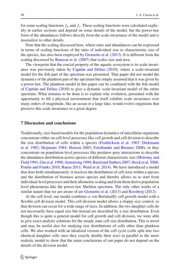
x < (1 + δ)/2. This means that p(w,w∗) = 0 for all w � wth(1 − δ)/2 andthat it is a differentiable function in the whole interval [0, w∗]. From the fact that∂p(w,w∗)/∂w < 0 when w > w+ we can conclude that the maximum of thisfunction will occur at some point wmax < w+ (Fig. 1).

0.4 0.6 0.8 1.0

0.0

0.2

0.4

0.6

0.8

1.0

x

Ψ(x

)

Fig. 1 The steady-state within-species size-distribution ψ(x), with constant mortality, growth parametervalues a = 0.7, b = 0.5, α = 0.85, β = 1, a division threshold of 0.7w∗ and rate K (w,w∗) given byEq. (4.14) with k(x) = 4(x − 0.7)2/(1 − x) and daughter cell sizes distributed uniformly between 0.4w∗and 0.6w∗

123


5 Predation by zooplankton

In the idealised model of cell division of Sect. 3 as well as in the more general modelof Sect. 4, we have seen that the allometric scaling of the death rate is a crucialingredient to the coexistence of multiple phytoplankton species living on one or a fewresources. The main cause of phytoplankton death is predation. Many species feed onphytoplankton, from unicellular organisms to whales. Even though a detailedmodel ofthe marine ecosystem would have to include these very many types of grazers as wellas their predators, in order to keep the model simple—and at the same time to illustratehow predation can provide the sort of death rate necessary for coexistence—we willfocus only on unicellular zooplankton.

We will denote the density of zooplankton cells by z(w,w∗, t), so that the numberof cells in a unit volume with a maximum size between w∗ and w∗ + dw∗ that at timet have a size between w and w + dw is z(w,w∗, t)dwdw∗.

To model predation, we introduce a new rate function S(w,w′): the rate at whicha given predator cell of size w preys on a given prey cell of size w′. This rate couldalso be allowed to depend on the specific predator and prey species through w∗ andw′∗. However, this would introduce unnecessary notational complexity without addinganything qualitatively different to the discussion.

A common ansatz for this rate function in the literature is

S(w,w′) = wνs(w/w′). (5.1)

The second factor is a kernel that selects the preferred prey size relative to the sizeof the predator (Wirtz 2012). The power of w in front of it arises from the foragingstrategy, which is known to depend allometrically on cell size (DeLong and Vasseur2012).

The mortality rate due to predation is obtained by integrating the contributionsfrom all predators. For the sake of completeness, a background death due to othersources—for which we will adopt the allometric scaling (3.10)—will be added. Thuswe set

M(w,w∗, t) =∫ ∞

0S(w′, w)zc(w

′, t) dw′ + w−ξ∗ mb(w/w∗), (5.2)

where the zooplankton community spectrum is defined as

zc(w, t) =∫ ∞

0z(w,w∗, t) dw∗. (5.3)

Zooplankton abundance is described by an equation similar to Eq. (2.10),

∂

∂tz(w,w∗, t) = − ∂

∂w

[Gz(w,w∗, t)z(w,w∗, t)

]

+ 2∫ ∞

0Q(w|w′)Kz(w

′, w∗, t)z(w′, w∗, t) dw′

− Kz(w,w∗, t)z(w,w∗, t) − M(w,w∗, t)z(w,w∗, t),

(5.4)

123


where the growth rate is now

Gz(w,w∗, t) =∫ ∞

0S(w,w′)εw′ [pc(w′, t) + zc(w

′, t)]dw′ − bw1−ξ∗

(w

w∗

)β

,

(5.5)with the phytoplankton community spectrum defined as

pc(w, t) =∫ ∞

0p(w,w∗, t) dw∗. (5.6)

The first term in (5.5) represents the uptake of nutrients from predation. The fac-tor ε expresses the efficiency with which prey biomass w′ is converted into predatorbiomass. It is assumed that predators prey indiscriminately on all species of cells,whether zoo- or phytoplankton. The second term accounts for the metabolic con-sumption. Although we choose this to be the same as for phytoplankton cells [seeEq. (2.5)], substituting different values for b and β would not change the results of themodel qualitatively.

The steady state of themodel we have just introduced has an important property thatis the main result of this paper, namely that, under the assumptions of the model—in particular the allometric scalings assumed for for the phytoplankton growth rate[Eq. (2.6)] as well as for the predation kernel [Eq. (5.1)], the death rate M(w,w∗) andthe zooplankton growth rate Gz(w,w∗) scale allometrically as

M(λw, λw∗) = λ−ξ M(w,w∗) and Gz(λw, λw∗) = λ1−ξGz(w,w∗) (5.7)

if, and only if, the community spectra of the phyto- and zooplankton scale as

pc(λw) = λ−γ pc(w) and zc(λw) = λ−γ zc(w), (5.8)

with γ = 1 + ν + ξ .The importance of this result lies in the fact that, according to the discussion of

Sects. 3.2 [in the paragraph containing Eq. (3.10)] and 4.3 (second paragraph), thisallometric scaling of M(w,w∗) is a necessary and sufficient condition for the steadystate to exhibit a species-rich phytoplankton community, and similarly, given the scal-ing ofM(w,w∗), that ofGz(w,w∗) becomes then a necessary and sufficient conditionfor the steady state to exhibit a species-rich zooplankton community. Accordingly, theparadox of the plankton and the power-law size spectrum of the plankton communityare two manifestations of one single phenomenon—which also expresses itself in theallometric scaling of those two rates.

We will discuss this point further in Sect. 7, and devote the rest of this section toproving this result. If we substitute zc = z0w−γ within Eq. (5.2) we obtain

M(w,w∗) = w−ξ∗ m(w/w∗), m(x) = mb(x) + z0 x

−ξ

∫ ∞

0y−ξ−1s(y) dy. (5.9)

123


This trivially satisfies the required allometric scaling. If we substitute both pc =φ0w

−γ and zc = z0w−γ within (5.5) we arrive at

Gz(w,w∗) = w1−ξ∗

[apz

(w

w∗

)1−ξ

− b

(w

w∗

)β]

,

apz = ε(p0 + z0)∫ ∞

0xγ−3s(x) dx .

(5.10)

This also complies with the required allometric scaling.To prove the converse we impose the scaling M(λw, λw∗) = λ−ξ M(w,w∗) on

Eq. (5.2), which leads to

∫ ∞

0S(w′, λw)zc(w

′) dw′ = λ−ξ

∫ ∞

0S(w′, w)zc(w

′) dw′.

Changing the variable w′ = λu and using the scaling S(λw, λw′) = λνS(w,w′)derived from (5.1), this equation transforms into

λ1+ν

∫ ∞

0S(u, w)zc(λu) du = λ−ξ

∫ ∞

0S(w′, w)zc(w

′) dw′,

which holds if, and only if, zc(λw) = λ−γ zc(w) with γ = 1+ ν + ξ . Doing the samewith the zooplankton growth rate (5.5) amounts to imposing the scaling

∫ ∞

0S(λw,w′)w′[pc(w′) + zc(w

′)]dw′ = λ1−ξ

∫ ∞

0S(w,w′)w′[pc(w′)

+ zc(w′)]dw′,

which, using the same argument as above, leads to pc(λw) = λ−γ pc(w).An interesting by-product of this result is that the expressions for M(w,w∗) and

Gz(w,w∗) have the same scaling form as those introduced in the analysis of phy-toplankton in previous sections. Therefore we can obtain the steady state of the fullsystem doing similar calculations. We will discuss this steady state first as obtainedunder the idealised division assumption and then as obtained for the general model.

5.1 Steady state with idealised divisionprocess

We can again make the idealised division assumption that cells divide exactly atsize w∗ into two equal-size cells. As in the case of phytoplankton, this amounts tochoosing Kz(w,w∗, t) = Gz(w,w∗, t)δ(w − w∗) and Q(w|w′) = δ(w − w′/2),which transforms the population balance equation (2.10) into

∂

∂tz(w,w∗, t) = − ∂

∂w

[Gz(w,w∗, t)z(w,w∗, t)

] − M(w,w∗, t)z(w,w∗, t),(5.11)

123


valid in the interval w∗/2 � w � w∗, with the boundary condition

2Gz(w∗, w∗, t)z(w∗, w∗, t) = Gz(w∗/2, w∗, t)z(w∗/2, w∗, t). (5.12)

The expressions for the death and growth rates for zooplankton are formally thesame as those for phytoplankton. Therefore the steady state size distributions of speciesabundances are given by

p(w,w∗) = p(w∗, w∗)φp(w/w∗), z(w,w∗) = z(w∗, w∗)φz(w/w∗), (5.13)

where

φp(x) = a(N ) − b

a(N )xα − bxβexp

{∫ 1

x

m(y)

a(N )yα − byβdy

}, (5.14)

N being the steady state value of the nutrient concentration, and

φz(x) = apz − b

apzx1−ξ − bxβexp

{∫ 1

x

m(y)

apz y1−ξ − byβdy

}(5.15)

with apz given in Eq. (5.10).The overall species abundances p(w∗, w∗) and z(w∗, w∗) can be obtained through

Eqs. (5.3) and (5.6). For the phytoplankton, for instance, given that p(w,w∗) = 0 forw > w∗,

pc(w) =∫ ∞

w

p(w∗, w∗)φp(w/w∗) dx = w

∫ 1

0p

(w

x,w

x

)φp(x)

dx

x2.

Now, given the scaling pc(λw) = λ−γ pc(w), this equation implies that p(λw∗, λw∗)= λ−γ−1 p(w∗, w∗), i.e.,

p(w∗, w∗) = p0Ip(γ − 1)

w−γ−1∗ , (5.16)

in terms of the functions

Ip(η) =∫ 1

0xηφp(x) dx, Iz(η) =

∫ 1

0xηφz(x) dx . (5.17)

A similar argument yields

z(w∗, w∗) = z0Iz(γ − 1)

w−γ−1∗ . (5.18)

As in the case of phytoplankton alone, the level of nutrient at the steady state isdetermined by the boundary condition (3.13), which fixes the value of a(N ). There isa problem though. In this idealised version of a plankton community we are implicitly

123


assuming an infinite biomass, because we are not imposing any lower nor upper limiton the size of cells. This translates into an infinite nutrient uptake by the phytoplankton,

σ(N , p) = a(N )

θ

∫ ∞

0dw∗ w

1−α−ξ∗∫ w∗

0dw wα p(w,w∗)

= a(N )

θp0

Ip(α)

Ip(γ − 1)

∫ ∞

0dw∗ w

1−ξ−γ∗ ,

which will then require an infinite amount of nutrient to survive.In reality there will always be a minimum size wmin and a maximum size wmax , so

if we introduce the factor

Ξ =∫ wmax

wmin

dw∗ w1−ξ−γ∗ (5.19)

and assume that all resource-related quantities diverge proportional to Ξ , we canrescale those quantities accordingly, so that they stay finite also in the limit ofwmin →0 and wmax → ∞. Hence we introduce a renormalised nutrient concentration N =lim N/Ξ , where the limit takes wmin → 0 and wmax → ∞, and similarly with othervariables (a hat will henceforth denote these renormalised quantities). The dynamicsof the nutrient (2.12), in terms of renormalised quantities, becomes1

d N

dt= �(N ) − σ (N , p). (5.20)

Hence in the steady state the renormalised nutrient concentration satisfies �(N ) +σ (N , p), which can be rewritten as

p0 = θ�(N )Ip(γ − 1)

a(N )Ip(α). (5.21)

Once we have determined p0, the boundary condition

∫ 1

1/2

m(y)

apz y1−ξ − byβdy = log 2 (5.22)

yields apz , which in turns determines z0 via Eq. (5.10).

5.2 Steady state with general division process

We can introduce a division rate for zooplankton Kz(w,w∗) with similar propertiesas that for phytoplankton. The simplest choice is to take the same function—as itis conceivable that the dynamics of cell division does not depend on the feedingmechanism—or any other alternative, but in any case scaling (4.14) must hold for

1 In these expressions a(N ) = a∞ N/(r + N ) and �(N ) = �0(1 − N/N0).

123


Kz(w,w∗) as well. Also, we assume that the size distribution of daugher cells isdescribed by the same function Q(w|w′).

Then we can introduce a similar splitting for zooplankton abundance

z(w,w∗, t) ={zl(w,w∗, t), w ≥ w+,

zs(w,w∗, t), w ≤ w+,(5.23)

and write equations similar to (4.3) and (4.4). The steady state of those equations willbe given by

p(w,w∗) = p(w+, w∗)ψp(w/w∗), z(w,w∗) = z(w+, w∗)ψz(w/w∗), (5.24)

where

ψp(x) = a(N )( 1+δ

2

)α − b( 1+δ

2

)β

a(N )xα − bxβep(x)Θp(x), (5.25)

ep(x) = exp

{−

∫ x

1+δ2

k(y) + m(y)

a(N )yα − byβdy

}, (5.26)

h p(x) =∫ 1

wthw∗

k(y)ep(y)

a(N )yα − byβq

(x

y

)dy, (5.27)

Θp(x) =⎧⎨⎩1, x > 1+δ

2 ,∫ x

0

k(y)

ep(y)dy, x < 1+δ

2 ,(5.28)

and

ψz(x) = apz( 1+δ

2

)1−ξ − b( 1+δ

2

)β

apzx1−ξ − bxβez(x)Θz(x), (5.29)

ez(x) = exp

{−

∫ x

1+δ2

k(y) + m(y)

apz y1−ξ − byβdy

}, (5.30)

hz(x) =∫ 1

wthw∗

k(y)ez(y)

apz y1−ξ − byβq

(x

y

)dy, (5.31)

Θz(x) =⎧⎨⎩1, x > 1+δ

2 ,∫ x

0

k(y)

ez(y)dy, x < 1+δ

2 .(5.32)

Introducing the functions

Jp(η) =∫ 1

0xηψp(x) dx, Jz(η) =

∫ 1

0xηψz(x) dx, (5.33)

123


and reproducing the arguments of Sect. 5.1, we obtain

p(w+, w∗) = p0Jp(γ − 1)

w−γ−1∗ , z(w+, w∗) = z0

Jz(γ − 1)w

−γ−1∗ , (5.34)

with

p0 = θ�(N )Jp(γ − 1)

a(N )Jp(α)(5.35)

and z0 derived from (5.10), with apz obtained through the boundary condition

∫ 1+δ2

0

hz(y)

ez(y)dy = 1. (5.36)

What we can conclude from the analysis of the last two sections is that only twosteady states are possible in this system in which zooplankton predate on phytoplank-ton: (a) a collapsed community in which at most a few species of phytoplankton—andpossibly of zooplankton—survive; or (b) a communitymade of a continuum of speciesof sizes 0 < w < ∞ that align on a single power law spectrum, with an exponent γ

determined by the allometry of the phytoplankton growth rate and of the zooplanktonpredation rate.

It is interesting to realise how the different facts assemble together to yield thisresult. On the one hand, as zooplankton predation is the main cause of phytoplank-ton mortality, in order for several phytoplankton species to coexist the zooplanktoncommunity is forced to distribute their abundances on a power law. In turn, zooplank-ton grow by predation, and in order for several zooplankton species to coexist thephytoplankton community is forced to lie on the same power law. We see then thatboth communities sustain each other, and that biodiversity is both the cause and theconsequence of the power law size spectrum.

6 Scale invariance

In the last paragraph of Sect. 5 we gave an intuitive explanation of why both thephytoplankton and the zooplankton spectrum have to follow a power law in the steady-state. There is also a more formal explanation that we would like to exhibit in thissection: the steady-state equations are scale-invariant in the sense that if an abundancespectrum p(w,w∗), z(w,w∗) is a solution of the steady-state equations for some levelof nutrient N , then so is the scale-transformed spectrum

pλ(w,w∗) = λγ+1 p(λw, λw∗), zλ(w,w∗) = λγ+1z(λw, λw∗), (6.1)

for any positive λ. Thus solutions come in one-parameter families. The steady-statehowever is expected to be unique, and this implies that it must be scale invariant, whichin turn implies that it must be of the power-law form

p(w,w∗) = w−γ−1∗ f p(w/w∗) and z(w,w∗) = w

−γ−1∗ fz(w/w∗) (6.2)

123


for some scaling functions f p and fz . These scaling functions were calculated explic-itly in earlier sections and depend on some details of the model, but the power-lawform of the abundances follows directly from the scale-invariance of the model and isinsensitive to other details.

Note that the scaling discussed here, where rates and abundances can be expressedin terms of scaling functions of the ratio of individual size to characteristic size ofthe species, has also been employed by Giometto et al. (2013). It is different from thescaling discussed by Banavar et al. (2007) that scales size and area.

The viewpoint that the crucial property of the aquatic ecosystem is its scale invari-ance was previously taken by Capitán and Delius (2010), where a scale-invariantmodel for the fish part of the spectrum was presented. That paper did not model thedynamics of the plankton part of the spectrum but simply assumed that it was given bya power-law. The plankton model in this paper can be combined with the fish modelof Capitán and Delius (2010) to give a dynamic scale-invariant model of the entirespectrum. What remains to be done is to explain why evolution, presented with theopportunity to fill a physical environment that itself exhibits scale invariance overmany orders of magnitude, like an ocean or a large lake, would evolve organisms thatpreserve this scale invariance to a great degree.

7 Discussion and conclusions

Traditionally, size-based models for the population dynamics of unicellular organismsconcentrate either on cell-level processes like cell growth and cell division to describethe size distribution of cells within a species (Fredrickson et al. 1967; Diekmannet al. 1983; Heijmans 1984; Henson 2003; Friedlander and Brenner 2008), or theyconcentrate on population-level processes like predator–prey interactions to describethe abundance distribution across species of different characteristic size (Moloney andField 1991;Gin et al. 1998;Armstrong 1999;Baird andSuthers 2007; Stock et al. 2008;Poulin and Franks 2010; Banas 2011; Ward et al. 2014). We have introduced a modelthat does both simultaneously: it resolves the distribution of cell sizes within a speciesand the distribution of biomass across species and thereby allows us to start fromindividual-level processes and their allometric scaling and from themderive populationlevel phenomena like the power-law Sheldon spectrum. The only other works of asimilar nature that we are aware of are Giometto et al. (2013) and Rossberg (2012).

At the cell level, our model combines a von Bertalanffy cell growth model with aflexible cell division model. This cell division model allows a sloppy size control, sothat division can occur for a wide range of sizes. In addition, the two daughter cells donot necessarily have equal size but instead are described by a size distribution. Eventhough this is quite a general model for cell growth and cell division, we were ableto give exact analytic solutions for the steady state cell size distribution. This is noveland may be useful also for studying size distributions of cells other than planktoncells. We also worked with an idealised version of the cell cycle (cells split into twoidentical daughter cells once they exactly double their size) in parallel to the morerealistic model to show that the main conclusions of our paper do not depend on thedetails of the division model.

123


The most important aspect of our model is the coupling of the growth of a predatorcell to the death of a smaller prey cell. This makes the cell growth rate depend onthe abundance of prey and the cell death rate depend on the abundance of predators,leading to a non-linear model. It is remarkable that, in spite of this non-linearity, thiscoupling together of cells of all species allows an exact steady-state solution givingthe size distributions for a continuum of coexisting species.

The model has the property that, at steady state, the coexistence of multiple uni-cellular plankton species and the Sheldon power-law size spectrum are two differentmanifestations of just one single phenomenon—‘two sides of the same coin’. Thisconclusion rests very much on the allometry of the four rates involved: the growthrates of phyto- and zooplankton, the death rate, and the predation kernel. The first andlast of these allometries are supported by empirical data and have specified allometricexponents. However, the allometries of the zooplankton growth and death rates have toemerge from the predator–prey interactions at steady state, and are technical outcomesof our modelling. In summary, one can assume in the model any one of the followingproperties: (a) allometry of the rates, (b) coexistence of multiple species, and (c) apower-law community size spectrum. Then, from this, the other two properties can bederived.

While we have been able to show analytically in this paper that the model predicts acoexistence steady state that agrees with the Sheldon spectrum, we have not discussedthe stability of this steady state against small perturbations. Due to the complicatedform of the steady state solution, an analytic stability analysis is not feasible. Wehave therefore performed the numerical calculations and have reported on them ina less analytically demanding paper (Law et al. 2016). The numerical results showthat additional stabilising terms, like for example an extra density dependence ofthe predation rate, need to be added to the model to stabilise the steady state. Thisis in agreement with observations in Maury and Poggiale (2013, section 4.2). Asthose stabilising terms are reduced, the system undergoes a Hopf bifurcation duringwhich the steady-state becomes unstable and the new attractor is an oscillatory statedescribing waves of biomass moving up the size spectrum. When averaged over time,these oscillations average out to a power-law abundance.

Our analyticalmodel presented in this paper is trait-based rather than species-based,whichmeans that, rather than taking afinite set of species, it uses a continuumof speciesdistinguished by a continuous trait variable, in our case the maximum size of a cellof that species. All analytical results in this paper very much rely on the existence ofthis continuum of species, which is clearly an idealisation of a real aquatic ecosystemthat can only contain a finite set of species. In that case the community abundancecan never be an exact power law, and therefore also the resulting allometric scalingcan not be exact. One may wonder whether the qualitative results of this paper willcontinue to apply.

To test that, we have carried out numerical simulations of a version of the model(Law et al. 2016) with a finite number of species. A single zooplankton species feedingon an assemblage of twenty phytoplankton species drives its phytoplankton prey tovery low densities while on the path to extinction itself, leaving a community farfrom being described by a Sheldon spectrum. However, increasing the number ofzooplankton species to nine, distributed over a range of characteristic cell sizes, leads

123


to a community closer to a Sheldon spectrum. This is because with more zooplanktonspecies there is a closer approximation to the scaling needed for predation mortality inthe prey, in conjunction with the scaling needed for growth in the predator. Moreover,the steady state is locally asymptotically stable. This is quite different from the resultson randommatrices (May 1972; Allesina and Tang 2015) which have been interpretedin ecology as making it less likely for a community to be stable as species-richness andconnectance increase. Ecologists have looked extensively for more realistic networkstructures that could counter such instability in complex communities, e.g. Neutelet al. (2002), Neutel et al. (2007), Neutel and Thorne (2014), James et al. (2015) andJacquet et al. (2016). Our results in Law et al. (2016) suggest that stable, unicellular,ecological networks with Sheldon-like structure cannot be achieved unless enoughspecies are present to generate approximations to the scalings in predation.

In previous models investigating the continuous coexistence of species, e.g., Gyl-lenberg and Meszéna (2005) and Sasaki (1997), it had been found that even when amodel has a coexistence steady state that is dynamically stable, this steady state isunstable against any small structural change to the model, and regions of exclusiondevelop in trait space in which no species can exist. However, the results in Law et al.(2016) show that our model does not suffer from this structural instability. When wego from the exact power-law death and growth rates of the continuous model to theapproximate power-law in the presence of a finite number of species, the steady-stateremains stable and the abundance of these species still approximately follows theSheldon spectrum power law. How much of this structural stability is due to the extradensity dependence in the predation rate and how much of it is due to the fact that weexplicitly model the growth of individuals whereas previous works assumed that allindividuals of a species had the same size, remains to be investigated.

Our model works with a single trait variable. It ignores all other characteristicsthat distinguish different species, except whether it is an autotroph or a heterotroph.Clearly the model could be made more realistic by also distinguishing between differ-ent functional types, for example between diatoms and dinoflagelates. Also, it wouldbe easy to include mixotrophs without changing the conclusions of our model. How-ever we wanted our model to be the simplest conceptual model that clarifies howcoexistence on a Sheldon spectrum emerges. For the same reason, we included onlya single resource described by a very simple equation, whereas in reality the resourcedynamics are complicated and very seasonal.

One question that we have not addressed in this paper is the reason for the observedallometric scaling of the phytoplankton growth rate and the predation rate. As theseare at the basis of our derivation of coexistence and the Sheldon spectrum, finding anexplanation for them would be very interesting. The allometry of the phytoplanktongrowth rate may possibly be imposed by physical constraints. Allometric scaling hasbeen studied a lot over the last 30 years, startingwith the classics (Calder 1984; BonnerandMcMahon 1983; Schmidt-Nielsen 1984) andwith important contributions byWestet al. (1997), Banavar et al. (1999), Banavar et al. (2014), Kooijman (2010) and manyothers.

The predation kernel, on the other hand, combines two ingredients: a preferred preysize and a foraging term. Although there may also be physical constraints for the latter,both ingredients are to a great extend behavioural—hence subject to evolution. Take the

123


preference for a prey size, for instance. It is hard to believe that if the abundance of thepreferred prey is seriously depleted the predatorwill not adapt its consumption habits tokeep a sufficient food supply. We believe that, instead of an input, the predation kernelshould be an emergent feature, consequence of an underlying evolutionary principlethat guides efficient predation habits. We have to leave this interesting question for thefuture.

Acknowledgements JAC was supported by the Spanish mobility Grant PRX12/00124 and ProjectFIS2015-64349-P (MINECO/FEDER, UE). GWD and RLwere supported by EUGrant 634495MINOUWH2020-SFS-2014-2015.

Open Access This article is distributed under the terms of the Creative Commons Attribution 4.0 Interna-tional License (http://creativecommons.org/licenses/by/4.0/), which permits unrestricted use, distribution,and reproduction in any medium, provided you give appropriate credit to the original author(s) and thesource, provide a link to the Creative Commons license, and indicate if changes were made.

Appendix: Check of scale-invariance of steady-state equations

In this appendix we will verify our claim that the pair of functions

pλ(w,w∗) = λγ+1 p(λw, λw∗), zλ(w,w∗) = λγ+1z(λw, λw∗), (7.1)

whereγ = 1 + ν + ξ, (7.2)

solve steady-state equations provided the original functions p(w,w∗), z(w,w∗) dofor the same nutrient value N .

The steady state equations, obtained by setting the time derivative to zero in thedynamical equations (2.10) for p(w,w∗), (5.4) for z(w,w∗), and (5.20) for N are

∂

∂w

[Gp(w,w∗)p(w,w∗)

] =2∫ w∗

0Q(w|w′)K (w′, w∗)p(w′, w∗) dw′

− K (w,w∗)p(w,w∗) − M(w,w∗)p(w,w∗). (7.3)

∂

∂w

[Gz(w,w∗)z(w,w∗)

] =2∫ ∞

0Q(w|w′)Kz(w

′, w∗)z(w′, w∗) dw′

− Kz(w,w∗)z(w,w∗) − M(w,w∗)z(w,w∗), (7.4)

�(N ) =σ (N , p). (7.5)

123

http://creativecommons.org/licenses/by/4.0/


To check that pλ(w,w∗), zλ(w,w∗) solve these equations we simply substitute them.Let us start with (7.3) and consider each term individually. The left-hand side gives

∂

∂w

[Gp(w,w∗)pλ(w,w∗)

] = ∂

∂w

[Gp(w,w∗)λγ+1 p(λw, λw∗)

]

= λ∂

∂(λw)

[λξ−1Gp(λw, λw∗)λγ+1 p(λw, λw∗)

]

= λγ+1+ξ ∂

∂(λw)

[Gp(λw, λw∗)p(λw, λw∗)

],

(7.6)where we used the scaling property (2.6) of the growth rate Gp(w,w∗). The first termon the right-hand side of (7.3) gives

2∫ w∗

0Q(w|w′)K (w′, w∗)pλ(w

′, w∗) dw′

= 2∫ λw∗

0λQ(λw|λw′)λξ K (λw′, λw∗)λγ+1 p(λw′, λw∗) λ−1d(λw′)

= λγ+1+ξ2∫ λw∗

0Q(λw|λw′)K (λw′, λw∗)p(λw′, λw∗) d(λw′),

(7.7)

where we used the scaling properties (2.8) and (3.5). The second term gives

−K (w,w∗)pλ(w,w∗) = −λξ K (λw, λw∗)λγ+1 p(λw, λw∗)= −λγ+1+ξ K (λw, λw∗)p(λw, λw∗)

(7.8)

again due to the scaling property (3.5) of the division rate. Finally, using the expression(5.2) for the mortality rate, the last term gives

−M(w,w∗)pλ(w,w∗) = −[∫ ∞

0S(w′, w)

∫ ∞

0zλ(w

′, w′∗) dw′∗ dw′

+w−ξ∗ mb(w/w∗)

]pλ(w,w∗)

= −[ ∫ ∞

0λ−νS(λw′, λw)

∫ ∞

0λγ+1z(λw′, λw′∗) λ−1d(λw′∗) λ−1d(λw′)

+ λξ (λw∗)−ξmb(λw/λw∗)]λγ+1 p(λw, λw∗)

= −λγ+1+ξ M(λw, λw∗)pλ(λw, λw∗).

(7.9)

We substituted both pλ and zλ, used the scaling property of the predation rate S(w,w′)that follows from Eq. (5.1) and the relation (7.2) between the exponents.

Putting these four terms back together, we see that the resulting equation is the sameas the original equation evaluated at scaledweights λw and λw∗, up to an overall factor

123


of λγ+1+ξ . Given that the original equation holds for all weightsw andw∗, this showsthat the transformed equation is equivalent to the original one, establishing its scaleinvariance.

In the Eq. (7.4) for the zooplankton abundance the left-hand side involves thezooplankton growth rate given in Eq. (5.5) and we first determine its behaviour whenpλ and zλ replace the original functions:

Gz(w,w∗) =∫ ∞

0S(w,w′)εw′

[∫ ∞

0(pλ(w

′, w′∗) + zλ(w′, w′∗))dw′∗

]dw′

− bw1−ξ∗(

w

w∗

)β

=∫ ∞

0λ−νS(λw, λw′)ελ−1(λw′)

[∫ ∞

0λγ+1(p(λw′, λw′∗)

+z(λw′, λw′∗))λ−1d(λw′∗)]λ−1d(λw′)

− bλ−1+ξ (λw∗)1−ξ

(λw

λw∗

)β

= λξ−1Gz(λw, λw∗).(7.10)

Thus under the scale transformation the left-hand side of the zooplankton equation(7.4) becomes

∂

∂w

[λξ−1Gz(λw, λw∗)λγ+1z(λw, λw∗)

]

= λγ+1+ξ ∂

∂(λw)

[Gz(λw, λw∗)z(λw, λw∗)

].

(7.11)

The terms on the right-hand side transform just like those in the phytoplantkon equa-tion. So againwe find that the transformed equation is the same as the original equationat rescaled weights up to an overall factor of λγ+1+ξ .

Finally, in the renormalised resource equation (7.5) the left-hand side does notdepend on weights or plankton abundances, so is invariant under the scale transfor-mation. The right hand side transforms to

σ (N , pλ) = lima(N )

θ

∫ wmaxwmin

w1−α−ξ∗

∫ w∗0 wα pλ(w,w∗)dwdw∗∫ wmax

wminw

1−ξ−γ∗ dw∗

= lima(N )

θ

∫ λwmaxλwmin

λ−1+α+ξ (λw∗)1−α−ξ∫ λw∗0 λ−α(λw)αλγ+1 p(λw, λw∗)λ−1d(λw)λ−1d(λw∗)∫ λwmax

λwminλ−1+ξ+γ (λw∗)1−ξ−γ λ−1d(λw∗)

= σ (N , p)(7.12)

and thus is also invariant, meaning the entire equation is invariant. This completes theproof that all the steady-state equations are scale-invariant.

123


References

Allesina S, Tang S (2015) The stability–complexity relationship at age 40: a random matrix perspective.Popul Ecol 57(1):63–75

Andersen KH, Beyer JE (2006) Asymptotic size determines species abundance in the marine size spectrum.Am Nat 168:54–61

Armstrong RA (1999) Stable model structures for representing biogeochemical diversity and size spectrain plankton communities. J Plankton Res 21(3):445–464

Baird ME, Suthers IM (2007) A size-resolved pelagic ecosystem model. Ecol Model 203(3):185–203Banas NS (2011) Adding complex trophic interactions to a size-spectral planktonmodel: emergent diversity

patterns and limits on predictability. Ecol Model 222(15):2663–2675Banavar JR, Maritan A, Rinaldo A (1999) Size and form in efficient transportation networks. Nature

399(6732):130–132Banavar JR, Damuth J, Maritan A, Rinaldo A (2007) Scaling in ecosystems and the linkage of macroeco-

logical laws. Phys Rev Lett 98(6):068,104Banavar JR, Cooke TJ, Rinaldo A, Maritan A (2014) Form, function, and evolution of living organisms.

PNAS 111(9):3332–3337Benoît E, Rochet MJ (2004) A continuous model of biomass size spectra governed by predation and the

effects of fishing. J Theor Biol 226:9–21Bonner JT, McMahon TA (1983) On size and life. Scientific American Library, New YorkCalder WA (1984) Size, function, and life history. Courier Corporation, North ChelmsfordCamacho J, Solé RV (2001) Scaling in ecological size spectra. Eurphys Lett 55:774–780Capitán JA, Delius GW (2010) Scale-invariant model of marine population dynamics. Phys Rev E

81:061,901Datta S, Delius GW, Law R (2010) A jump-growth model for predator-prey dynamics: derivation and

application to marine ecosystems. Bull Math Biol 72:1361–1382Datta S, Delius GW, Law R, Plank MJ (2011) A stability analysis of the power-law steady state of marine

size spectra. J Math Biol 63:779–799DeLong JP, Vasseur DA (2012) Size-density scaling in protists and the links between consumer–resource

interaction parameters. J Anim Ecol 81:1193–1201Diekmann O, Lauwerier HA, Aldenberg T, Metz JAJ (1983) Growth, fission and the stable size distribution.

J Math Biol 18:135–148Fox JW (2013) The intermediate disturbance hypothesis should be abandoned. Trends Ecol Evol 28:86–92Fredrickson AG, Ramkrishna D, Tsuchyia HM (1967) Statistics and dynamics of procaryotic cell popula-

tions. Math Biosci 1:327–374Friedlander T, Brenner N (2008) Cellular properties and population asymptotics in the population balance

equation. Phys Rev Lett 101:018,104Gaedke U (1992) The size distribution of plankton biomass in a large lake and its seasonal variability.

Limnol Oceanogr 37(6):1202–1220Gin KYH, Guo J, Cheong HF (1998) A size-based ecosystem model for pelagic waters. Ecol Model

112(1):53–72Giometto A, Altermatt F, Carrara F, Maritan A, Rinaldo A (2013) Scaling body size fluctuations. Proc Nat

Acad Sci USA 110:4646–4650Guiet J, Poggiale JC, Maury O (2016) Modelling the community size-spectrum: recent developments and

new directions. Ecol Model 337:4–14Gyllenberg M, Meszéna G (2005) On the impossibility of coexistence of infinitely many strategies. J Math

Biol 50(2):133–160Hartvig M, Andersen KH, Beyer JE (2011) Food web framework for size-structured populations. J Theor

Biol 272:113–122Heijmans HJAM (1984) On the stable size distribution of populations reproducing by fission into two

unequal parts. Math Biosci 72:19–50Henson MA (2003) Dynamic modeling of microbial cell populations. Curr Opin Biotechnol 14:460–467Herbert D, Elsworth R, Telling RC (1956) The continuous culture of bacteria; a theoretical and experimental

study. J Gen Microbiol 14:601–622Hutchinson G (1961) The paradox of the plankton. Am Nat 95:137–145Jacquet C,Moritz C,Morissette L, Legagneux P,Massol F, Archambault P, Gravel D (2016) No complexity–

stability relationship in empirical ecosystems. Nat Commun 7:12,573

123


James A, Plank MJ, Rossberg AG, Beecham J, Emmerson M, Pitchford JW (2015) Constructing randommatrices to represent real ecosystems. Am Nat 185(5):680–692

Kempes CP, Dutkiewicz S, Follows MJ (2011) Growth, metabolic partitioning, and the size of microorgan-isms. Proc Natl Acad Sci USA 109:495–500

Kooijman SALM (2010) Dynamic energy budget theory for metabolic organisation. Cambridge UniversityPress, Amsterdam

Law R, Cuesta JA, Delius G (2016) Plankton: the paradox and the power law. arXiv:1705.05327 [q-bio.PE]Leibold MA (1996) Graphical model of keystone predators in food webs: trophic regulation of abundance,

incidence, and diversity patterns in communities. Am Nat 147:784–812Marañón E, Cermeño P, López-Sandoval DC, Rodríguez-Ramos T, Sobrino C, Huete-Ortega M, Blanco

JM, Rodríguez J (2013) Unimodal size scaling of phytoplankton growth and the size dependence ofnutrient uptake and use. Ecol Lett 16:371–379

Maury O, Poggiale JC (2013) From individuals to populations to communities: a dynamic energy budgetmodel of marine ecosystem size-spectrum including life history diversity. J Theor Biol 324:52–71

May RM (1972) Will a large complex system be stable? Nature 238:413–414Moloney CL, Field JG (1991) The size-based dynamics of plankton food webs I: a simulation model of

carbon and nitrogen flows. J Plankton Res 13(5):1003–1038Neutel AM, Heesterbeek JAP, de Ruiter PC (2002) Stability in real food webs: weak links in long loops.

Science 296(5570):1120–1123Neutel AM, Heesterbeek JAP, van de Koppel J, Hoenderboom G, Vos A, Kaldeway C, Berendse F, de

Ruiter PC (2007) Reconciling complexity with stability in naturally assembling food webs. Nature449(7162):599–602

Neutel AM, ThorneMA (2014) Interaction strengths in balanced carbon cycles and the absence of a relationbetween ecosystem complexity and stability. Ecol Lett 17(6):651–661

Platt T, Denman K (1977) Organisation in the pelagic ecosystem. Helgol Mar Res 30:575–581Poulin FJ, Franks PJS (2010) Size-structured planktonic ecosystems: constraints, controls and assembly

instructions. J Plankton Res 32(8):1121–1130Powell EO (1964) A note on Koch & Schaechters hypothesis about growth and fission of bacteria. J Gen

Microbiol 37:231–249Quiñones RA, Platt T, Rodríguez J (2003) Patterns of biomass-size spectra from oligotrophic waters of the

northwest atlantic. Prog Oceanogr 57:405–427RossbergAG (2012)A complete analytic theory for structure and dynamics of populations and communities

spanningwide ranges in body size. In: JacobUte,WoodwardGuy (eds)Advances in ecological researchglobal change in multispecies systems part 1, vol 46. Academic Press, London, pp 427–521

Roy S, Chattopadhyay J (2007) Towards a resolution of ‘the paradox of the plankton’: a brief overview ofthe proposed mechanisms. Ecol Complex 4:26–33

San Martin E, Harris RP, Irigoien X (2006) Latitudinal variation in plankton size spectra in the AtlanticOcean. Deep-Sea Res Pt II 53(14):1560–1572

Sasaki A (1997) Clumped distribution by neighbourhood competition. J Theor Biol 186(4):415–430Schmidt-Nielsen K (1984) Scaling: why is animal size so important? Cambridge University Press, Cam-

bridgeSheldon RW, Prakash A, Sutcliffe WH (1972) The size distribution of particles in the ocean. Limnol

Oceanogr 17:327–340SheldonRW,Kerr S (1972) The population density ofmonsters in LochNess. LimnolOceanogr 17:796–799SilvertW, Platt T (1978) Energy flux in the pelagic ecosystem: a time-dependent equation. Limnol Oceanogr

23:813–816SilvertW, Platt T (1980) Dynamic energy-flowmodel of the particle size distribution in pelagic ecosystems.

In: Kerfoot WC (ed) Evolution and ecology of zooplankton communities. New England UniversityPress, Hanover, pp 754–763

Sprules WG, Barth LE, Giacomini H (2016) Surfing the biomass size spectrum: some remarks on history,theory, and application. Can J Fish Aquat Sci 73(4):477–495

Stock CA, Powell TM, Levin SA (2008) Bottom-up and top-down forcing in a simple size-structuredplankton dynamics model. J Mar Syst 74(1):134–152

Thingstad TF, Lignell R (1997) Theoretical models for the control of bacterial growth rate, abundance,diversity and carbon demand. Aquat Microb Ecol 13:19–27

Tyson JJ, Diekmann O (1986) Sloppy size control of the cell division cycle. J Theor Biol 118:405–426

123

http://arxiv.org/abs/1705.05327


Våge S, Storesund JE, Giske J, Thingstad TF (2014) Optimal defense strategies in an idealized microbialfood web under trade-off between competition and defense. PLoS ONE 9:e101,415

von Bertalanffy L (1957) Quantitative laws in metabolism and growth. Q Rev Biol 32:217–231Ward BA, Dutkiewicz S, Follows MJ (2014) Modelling spatial and temporal patterns in size-structured

marine plankton communities: topdown and bottomup controls. J Plankton Res 36(1):31–47West GB, Brown JH, Enquist BJ (1997) A general model for the origin of allometric scaling laws in biology.

Science 276(5309):122–126Winter C, Bouvier T, Weinbaue MG, Thingstad TF (2010) Trade-offs between competition and defense

specialists among unicellular planktonic organisms: the “killing the winner” hypothesis revisited.Microb Mol Biol Rev 74:42–57

Wirtz KW (2012) Who is eating whom? Morphology and feeding type determine the size relation betweenplanktonic predators and their ideal prey. Mar Ecol Prog Ser 445:1–12

123

sheldon spectrum and the plankton paradox: two sides of ... · coexistence of a continuum of...

Documents