Shear and tensile properties of cement-treated sands and their application to mitigation of liquefaction-induced damage Koseki, J. and Tsutsumi, Y. Institute of Industrial Science, University of Tokyo, Japan

Namikawa, T. Dept. of Civil Engineering, Kobe City College of Technology, Japan

Mihira, S. Integrated Geotechnology Institute, Corp., Japan

Salas-Monge, R. Costarican Institute of Electricity, Costa Rica

Sano, Y. Kyosei Corporation, Japan

Nakajima, S. Public Works Research Institute, Japan

Keywords: cement treatment, sand, shear property, tensile property, liquefaction

ABSTRACT: Results from a variety of laboratory tests on shear and tensile properties of cement-treated sands are summarized. These properties were found to depend not only on the amounts of cement but also on some other factors, including the moulding water contents in case of pre-mixed cement-treated sands. In plane strain compression tests, initiation of strain localization was observed at the peak shear stress states, which developed into a full shear band during the post-peak strain-softening stage. In bending tests, post-peak strain-softening behavior that was associated with strain localization was also observed in the tensile region. Based on these experimental data, an elasto-plastic model considering the post-peak strain-softening properties in shear and tensile regions was developed and applied to FE analyses. As a result, the discrepancy in the nominal tensile strengths obtained by different types of laboratory tests could be simulated reasonably. It became also possible to assess rationally the performance of lattice type ground improvement by in-situ cement mixing that was executed to mitigate liquefaction-induced damage. 1 INTRODUCTION

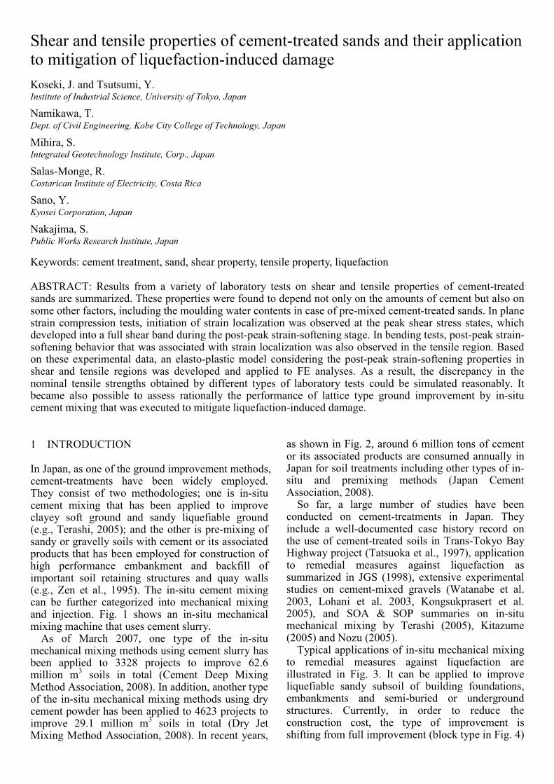
In Japan, as one of the ground improvement methods, cement-treatments have been widely employed. They consist of two methodologies; one is in-situ cement mixing that has been applied to improve clayey soft ground and sandy liquefiable ground (e.g., Terashi, 2005); and the other is pre-mixing of sandy or gravelly soils with cement or its associated products that has been employed for construction of high performance embankment and backfill of important soil retaining structures and quay walls (e.g., Zen et al., 1995). The in-situ cement mixing can be further categorized into mechanical mixing and injection. Fig. 1 shows an in-situ mechanical mixing machine that uses cement slurry.

As of March 2007, one type of the in-situ mechanical mixing methods using cement slurry has been applied to 3328 projects to improve 62.6 million m3 soils in total (Cement Deep Mixing Method Association, 2008). In addition, another type of the in-situ mechanical mixing methods using dry cement powder has been applied to 4623 projects to improve 29.1 million m3 soils in total (Dry Jet Mixing Method Association, 2008). In recent years,

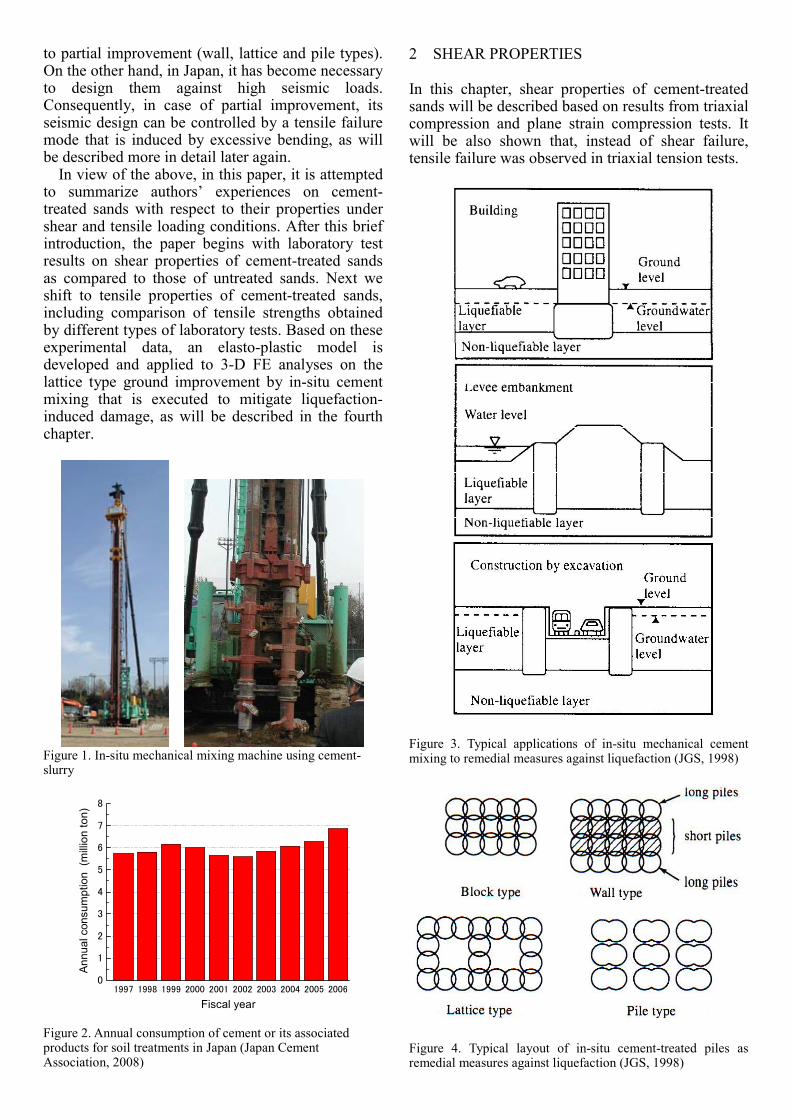
as shown in Fig. 2, around 6 million tons of cement or its associated products are consumed annually in Japan for soil treatments including other types of in-situ and premixing methods (Japan Cement Association, 2008).

So far, a large number of studies have been conducted on cement-treatments in Japan. They include a well-documented case history record on the use of cement-treated soils in Trans-Tokyo Bay Highway project (Tatsuoka et al., 1997), application to remedial measures against liquefaction as summarized in JGS (1998), extensive experimental studies on cement-mixed gravels (Watanabe et al. 2003, Lohani et al. 2003, Kongsukprasert et al. 2005), and SOA & SOP summaries on in-situ mechanical mixing by Terashi (2005), Kitazume (2005) and Nozu (2005).

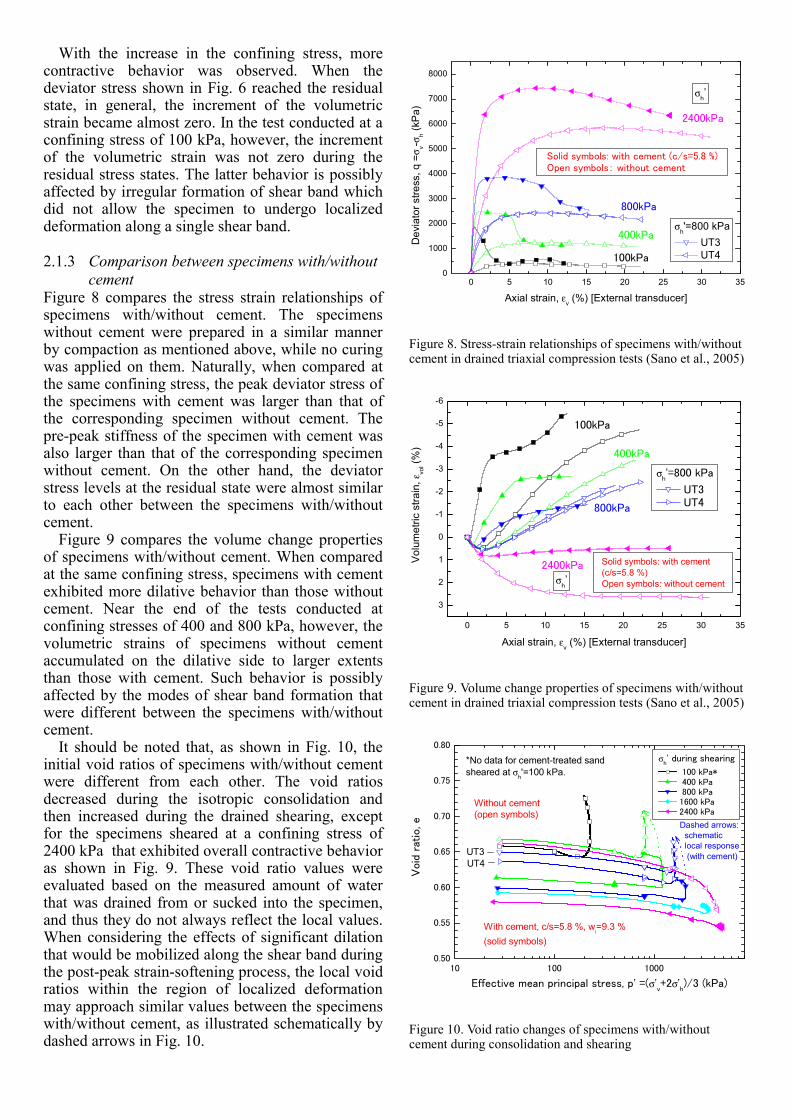
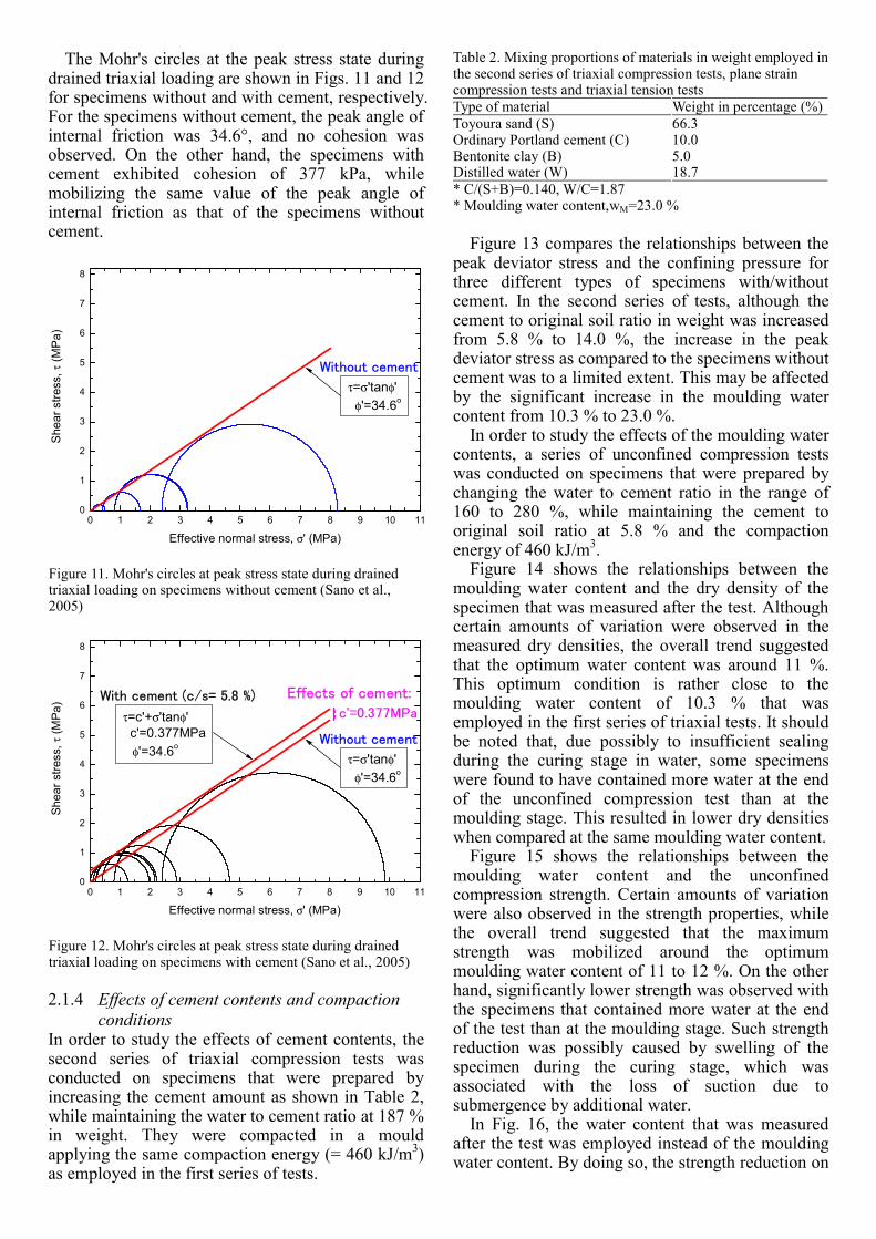
Typical applications of in-situ mechanical mixing to remedial measures against liquefaction are illustrated in Fig. 3. It can be applied to improve liquefiable sandy subsoil of building foundations, embankments and semi-buried or underground structures. Currently, in order to reduce the construction cost, the type of improvement is shifting from full improvement (block type in Fig. 4)

to partial improvement (wall, lattice and pile types). On the other hand, in Japan, it has become necessary to design them against high seismic loads. Consequently, in case of partial improvement, its seismic design can be controlled by a tensile failure mode that is induced by excessive bending, as will be described more in detail later again.

In view of the above, in this paper, it is attempted to summarize authors’ experiences on cement-treated sands with respect to their properties under shear and tensile loading conditions. After this brief introduction, the paper begins with laboratory test results on shear properties of cement-treated sands as compared to those of untreated sands. Next we shift to tensile properties of cement-treated sands, including comparison of tensile strengths obtained by different types of laboratory tests. Based on these experimental data, an elasto-plastic model is developed and applied to 3-D FE analyses on the lattice type ground improvement by in-situ cement mixing that is executed to mitigate liquefaction-induced damage, as will be described in the fourth chapter.

2 SHEAR PROPERTIES

In this chapter, shear properties of cement-treated sands will be described based on results from triaxial compression and plane strain compression tests. It will be also shown that, instead of shear failure, tensile failure was observed in triaxial tension tests.

Figure 3. Typical applications of in-situ mechanical cement mixing to remedial measures against liquefaction (JGS, 1998)

Figure 4. Typical layout of in-situ cement-treated piles asremedial measures against liquefaction (JGS, 1998)

Figure 1. In-situ mechanical mixing machine using cement-slurry

1997 1998 1999 2000 2001 2002 2003 2004 2005 20060

1

2

3

4

5

6

7

8

Annu

al c

onsu

mpt

ion

(mill

ion

ton)

Fiscal year Figure 2. Annual consumption of cement or its associated products for soil treatments in Japan (Japan Cement Association, 2008)

2.1 Triaxial compression tests

2.1.1 Test procedures The materials used were Toyoura sand (D50=0.18 mm, Uc=1.6), ordinary Portland cement, distilled water and a small amount of bentonite clay (wL=357 %, wp=25.1 %). Their mixing proportions as employed in the first series of triaxial compression tests are listed in Table 1. Table 1. Mixing proportions of materials in weight employed in the first series of triaxial compression tests Type of material Weight in percentage (%)Toyoura sand (S) 80.7 Ordinary Portland cement (C) 5.0 Bentonite clay (B) 5.0 Distilled water (W) 9.3 * C/(S+B)=0.058, W/C=1.87 * Moulding water content,wM=10.3%

They were put in a mould and compacted in five layers to prepare a cylindrical specimen having a diameter of 50 mm and a height of 100 mm. The compaction energy applied was 460 kJ/m3. The specimen was sealed and cured in water under room temperature for about seven days. The curing time was adjusted to be 168 hours at the start of shearing.

The triaxial cell employed is schematically shown in Fig. 5. It has a capacity of applying a cell pressure of 3 MPa and an axial load of 100 kN. After trimming, the specimen was placed on a pedestal that can slide freely on a horizontal plane. In order to reduce the possible effects of bedding error at the interfaces between the specimen and the top cap and pedestal, capping was made at both ends by using gypsum. The above free sliding of the pedestal was, therefore, required in order not to constrain the specimen deformation, in particular after the formation of shear band. To facilitate drainage, a side drain of filter paper was used.

The specimen was saturated by a combination of double-vacuuming (Ampadu and Tatsuoka, 1993) and back pressurizing to 196 kPa in the triaxial cell that is filled with water. The specimen was then consolidated isotropically under different levels of confining stresses in the range of 100 to 2400 kPa. After consolidation for 20 hours, the specimen was sheared at an axial strain rate of 0.01 %/min under drained condition.

2.1.2 Effects of confining stress Figure 6 compares the stress strain relationships of specimens consolidated under different confining stress levels. In the figure, the result from an unconfined compression test is also plotted. With the increase in the confining stress, the peak deviator stress increased, while the post-peak strain softening behavior became less remarkable. It should be noted that, since one test (CT4) at a confining stress of 200 kPa had to be terminated during shearing due to technical problems, another test (CT3) was conducted under similar conditions.

Figure 7 compares the volume change properties of specimens consolidated under different confining stress levels.

①

②

③④

⑤⑥

⑦

⑧

⑨

⑩

⑩

⑪

①

②

③④

⑤⑥

⑦

⑧

⑨

⑩

⑩

⑪

①Loading shaft②Clamp③Bearing ball box④Rubber O-ring⑤Acrylic pipe (φ:250mm, t:25mm)⑥Tie rod(φ:30mm)⑦Load cell (100kN)⑧Cap⑨Pedestal⑩⑩Bearing ballBearing ball⑪LDT

Figure 5. Apparatus for triaxial compression tests

0 5 10 15 20 25 30 350

1000

2000

3000

4000

5000

6000

7000

8000σ

h'

Dev

iato

r stre

ss, q

=σv-σ

h (kP

a)

Axial strain, εv (%) [External transducer]

2400kPa

1600kPa

800kPa

400kPa

200kPa100kPa0kPa

σh'=200 kPa:

CT3 CT4

c/s=5.8 %, wi=9.3 %

Figure 6. Stress-strain relationships of specimens with cement in drained triaxial compression tests under different confining stress levels (Sano et al., 2005)

-6

-5

-4

-3

-2

-1

0

1

0 5 10 15 20 25 30 35

σh'

c/s=5.8 %, wi=9.3 %100kPa

200kPa

400kPa

800kPa

1600kPa

2400kPa

Axial strain, εv (%) [External transducer]

Volu

met

ric s

train

, εvo

l (%)

σh'=200 kPa

CT3 CT4

Figure 7. Volume change properties of specimens with cement in drained triaxial compression tests under different confining stress levels (Sano et al., 2005)

With the increase in the confining stress, more contractive behavior was observed. When the deviator stress shown in Fig. 6 reached the residual state, in general, the increment of the volumetric strain became almost zero. In the test conducted at a confining stress of 100 kPa, however, the increment of the volumetric strain was not zero during the residual stress states. The latter behavior is possibly affected by irregular formation of shear band which did not allow the specimen to undergo localized deformation along a single shear band.

2.1.3 Comparison between specimens with/without cement

Figure 8 compares the stress strain relationships of specimens with/without cement. The specimens without cement were prepared in a similar manner by compaction as mentioned above, while no curing was applied on them. Naturally, when compared at the same confining stress, the peak deviator stress of the specimens with cement was larger than that of the corresponding specimen without cement. The pre-peak stiffness of the specimen with cement was also larger than that of the corresponding specimen without cement. On the other hand, the deviator stress levels at the residual state were almost similar to each other between the specimens with/without cement.

Figure 9 compares the volume change properties of specimens with/without cement. When compared at the same confining stress, specimens with cement exhibited more dilative behavior than those without cement. Near the end of the tests conducted at confining stresses of 400 and 800 kPa, however, the volumetric strains of specimens without cement accumulated on the dilative side to larger extents than those with cement. Such behavior is possibly affected by the modes of shear band formation that were different between the specimens with/without cement.

It should be noted that, as shown in Fig. 10, the initial void ratios of specimens with/without cement were different from each other. The void ratios decreased during the isotropic consolidation and then increased during the drained shearing, except for the specimens sheared at a confining stress of 2400 kPa that exhibited overall contractive behavior as shown in Fig. 9. These void ratio values were evaluated based on the measured amount of water that was drained from or sucked into the specimen, and thus they do not always reflect the local values. When considering the effects of significant dilation that would be mobilized along the shear band during the post-peak strain-softening process, the local void ratios within the region of localized deformation may approach similar values between the specimens with/without cement, as illustrated schematically by dashed arrows in Fig. 10.

0 5 10 15 20 25 30 350

1000

2000

3000

4000

5000

6000

7000

8000

σh'

Solid symbols: with cement (c/s=5.8 %)Open symbols： without cement

2400kPa

800kPa

400kPa

100kPa

Dev

iato

r stre

ss, q

=σ v-σ

h (kP

a)

Axial strain, εv (%) [External transducer]

σh'=800 kPa

UT3 UT4

Figure 8. Stress-strain relationships of specimens with/without cement in drained triaxial compression tests (Sano et al., 2005)

-6

-5

-4

-3

-2

-1

0

1

2

3

0 5 10 15 20 25 30 35

σh'

Solid symbols: with cement(c/s=5.8 %)Open symbols: without cement

2400kPa

800kPa

400kPa

100kPa

Axial strain, εv (%) [External transducer]

Vol

umet

ric s

train

, εvo

l (%)

σh'=800 kPa

UT3 UT4

Figure 9. Volume change properties of specimens with/without cement in drained triaxial compression tests (Sano et al., 2005)

10 100 10000.50

0.55

0.60

0.65

0.70

0.75

0.80

Dashed arrows: schematic local response (with cement)

UT4

With cement, c/s=5.8 %, wi=9.3 %(solid symbols)

Without cement(open symbols)

Void

rat

io, e

Effective mean principal stress, p' =(σ'v+2σ'

h)/3 (kPa)

σh' during shearing

100 kPa* 400 kPa 800 kPa 1600 kPa 2400 kPa

*No data for cement-treated sand sheared at σh'=100 kPa.

UT3

Figure 10. Void ratio changes of specimens with/without cement during consolidation and shearing

The Mohr's circles at the peak stress state during drained triaxial loading are shown in Figs. 11 and 12 for specimens without and with cement, respectively. For the specimens without cement, the peak angle of internal friction was 34.6°, and no cohesion was observed. On the other hand, the specimens with cement exhibited cohesion of 377 kPa, while mobilizing the same value of the peak angle of internal friction as that of the specimens without cement.

2.1.4 Effects of cement contents and compaction conditions

In order to study the effects of cement contents, the second series of triaxial compression tests was conducted on specimens that were prepared by increasing the cement amount as shown in Table 2, while maintaining the water to cement ratio at 187 % in weight. They were compacted in a mould applying the same compaction energy (= 460 kJ/m3) as employed in the first series of tests.

Table 2. Mixing proportions of materials in weight employed in the second series of triaxial compression tests, plane strain compression tests and triaxial tension tests Type of material Weight in percentage (%)Toyoura sand (S) 66.3 Ordinary Portland cement (C) 10.0 Bentonite clay (B) 5.0 Distilled water (W) 18.7 * C/(S+B)=0.140, W/C=1.87 * Moulding water content,wM=23.0 %

Figure 13 compares the relationships between the peak deviator stress and the confining pressure for three different types of specimens with/without cement. In the second series of tests, although the cement to original soil ratio in weight was increased from 5.8 % to 14.0 %, the increase in the peak deviator stress as compared to the specimens without cement was to a limited extent. This may be affected by the significant increase in the moulding water content from 10.3 % to 23.0 %.

In order to study the effects of the moulding water contents, a series of unconfined compression tests was conducted on specimens that were prepared by changing the water to cement ratio in the range of 160 to 280 %, while maintaining the cement to original soil ratio at 5.8 % and the compaction energy of 460 kJ/m3.

Figure 14 shows the relationships between the moulding water content and the dry density of the specimen that was measured after the test. Although certain amounts of variation were observed in the measured dry densities, the overall trend suggested that the optimum water content was around 11 %. This optimum condition is rather close to the moulding water content of 10.3 % that was employed in the first series of triaxial tests. It should be noted that, due possibly to insufficient sealing during the curing stage in water, some specimens were found to have contained more water at the end of the unconfined compression test than at the moulding stage. This resulted in lower dry densities when compared at the same moulding water content.

Figure 15 shows the relationships between the moulding water content and the unconfined compression strength. Certain amounts of variation were also observed in the strength properties, while the overall trend suggested that the maximum strength was mobilized around the optimum moulding water content of 11 to 12 %. On the other hand, significantly lower strength was observed with the specimens that contained more water at the end of the test than at the moulding stage. Such strength reduction was possibly caused by swelling of the specimen during the curing stage, which was associated with the loss of suction due to submergence by additional water.

In Fig. 16, the water content that was measured after the test was employed instead of the moulding water content. By doing so, the strength reduction on

0 1 2 3 4 5 6 7 8 9 10 110

1

2

3

4

5

6

7

8

τ=σ'tanφ' φ'=34.6o

Without cement

She

ar s

tress

, τ (M

Pa)

Effective normal stress, σ' (MPa) Figure 11. Mohr's circles at peak stress state during drained triaxial loading on specimens without cement (Sano et al., 2005)

0 1 2 3 4 5 6 7 8 9 10 110

1

2

3

4

5

6

7

8

c'=0.377MPa

τ=σ'tanφ' φ'=34.6o

Without cement

With cement (c/s= 5.8 %)

τ=c'+σ'tanφ' c'=0.377MPa φ'=34.6o

Shea

r stre

ss, τ

(MPa

)

Effective normal stress, σ' (MPa)

Effects of cement:

Figure 12. Mohr's circles at peak stress state during drained triaxial loading on specimens with cement (Sano et al., 2005)

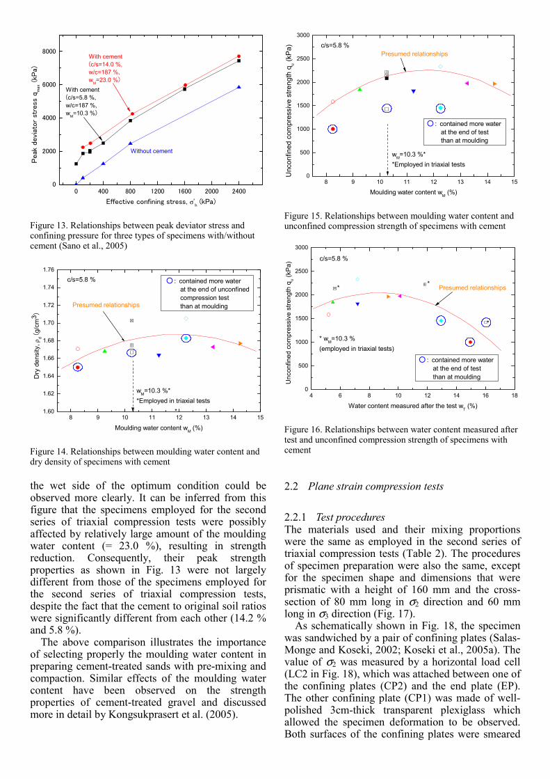
the wet side of the optimum condition could be observed more clearly. It can be inferred from this figure that the specimens employed for the second series of triaxial compression tests were possibly affected by relatively large amount of the moulding water content (= 23.0 %), resulting in strength reduction. Consequently, their peak strength properties as shown in Fig. 13 were not largely different from those of the specimens employed for the second series of triaxial compression tests, despite the fact that the cement to original soil ratios were significantly different from each other (14.2 % and 5.8 %).

The above comparison illustrates the importance of selecting properly the moulding water content in preparing cement-treated sands with pre-mixing and compaction. Similar effects of the moulding water content have been observed on the strength properties of cement-treated gravel and discussed more in detail by Kongsukprasert et al. (2005).

2.2 Plane strain compression tests

2.2.1 Test procedures The materials used and their mixing proportions were the same as employed in the second series of triaxial compression tests (Table 2). The procedures of specimen preparation were also the same, except for the specimen shape and dimensions that were prismatic with a height of 160 mm and the cross-section of 80 mm long in σ2 direction and 60 mm long in σ3 direction (Fig. 17).

As schematically shown in Fig. 18, the specimen was sandwiched by a pair of confining plates (Salas-Monge and Koseki, 2002; Koseki et al., 2005a). The value of σ2 was measured by a horizontal load cell (LC2 in Fig. 18), which was attached between one of the confining plates (CP2) and the end plate (EP). The other confining plate (CP1) was made of well-polished 3cm-thick transparent plexiglass which allowed the specimen deformation to be observed. Both surfaces of the confining plates were smeared

0 400 800 1200 1600 2000 24000

2000

4000

6000

8000With cement(c/s=14.0 %,w/c=187 %,w

M=23.0 %)

Peak

devi

ator

stre

ss q

max (kP

a)

Effective confining stress, σ'h (kPa)

With cement(c/s=5.8 %,w/c=187 %,wM=10.3 %)

Without cement

Figure 13. Relationships between peak deviator stress and confining pressure for three types of specimens with/without cement (Sano et al., 2005)

8 9 10 11 12 13 14 151.60

1.62

1.64

1.66

1.68

1.70

1.72

1.74

1.76

○： contained more water at the end of unconfined compression test than at moulding

wM=10.3 %**Employed in triaxial tests

c/s=5.8 %

*

Presumed relationships

Dry

den

sity

, ρd (g

/cm

3 )

Moulding water content wM (%)

Figure 14. Relationships between moulding water content and dry density of specimens with cement

8 9 10 11 12 13 14 150

500

1000

1500

2000

2500

3000

c/s=5.8 %Presumed relationships

○： contained more water at the end of test than at moulding

wM=10.3 %**Employed in triaxial tests

Unc

onfin

ed c

ompr

essi

ve s

treng

th q

u (kP

a)

Moulding water content wM (%)

Figure 15. Relationships between moulding water content and unconfined compression strength of specimens with cement

4 6 8 10 12 14 16 180

500

1000

1500

2000

2500

3000

* wM=10.3 % (employed in triaxial tests)

○： contained more water at the end of test than at moulding

*

* Presumed relationshipsU

ncon

fined

com

pres

sive

stre

ngth

qu (k

Pa)

Water content measured after the test wT (%)

*

c/s=5.8 %

Figure 16. Relationships between water content measured after test and unconfined compression strength of specimens with cement

with a thin layer of silicone grease to reduce the side friction, which was measured by two additional load cells (FrLC1 and FrLC2). To allow the movement of specimen in σ3 direction that was necessary for free development of a single shear band with a plane parallel to σ2 direction, the pedestal was mounted on a moving plate which in turn was lying on a set of two ball bearings.

After saturation, consolidation and application of an initial deviator stress in the horizontal direction to ensure good contact between the specimen and the confining plates, the specimen was sheared at an axial strain rate of 0.01 and 0.03 %/min, respectively, for monotonic and cyclic loadings.

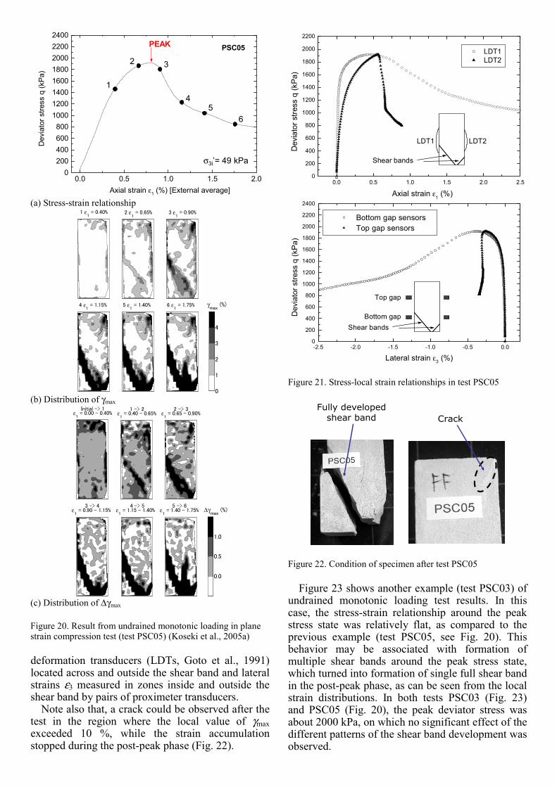
At different stages during shearing, as typically shown in Fig. 19, digital photographs of the specimen’s σ2 face were taken through the transparent plexiglass plate, where the rubber membrane covering the specimen had been imprinted with a series of points equally spaced every 5 mm. The horizontal and vertical

displacements of each point were read from the photographs, and the deformation at the center of each of the rectangular elements that were defined by the grid of points was calculated. Finally, distributions of the maximum shear strain (γmax=ε1-ε3) and its increment between specified states (∆γmax) were plotted.

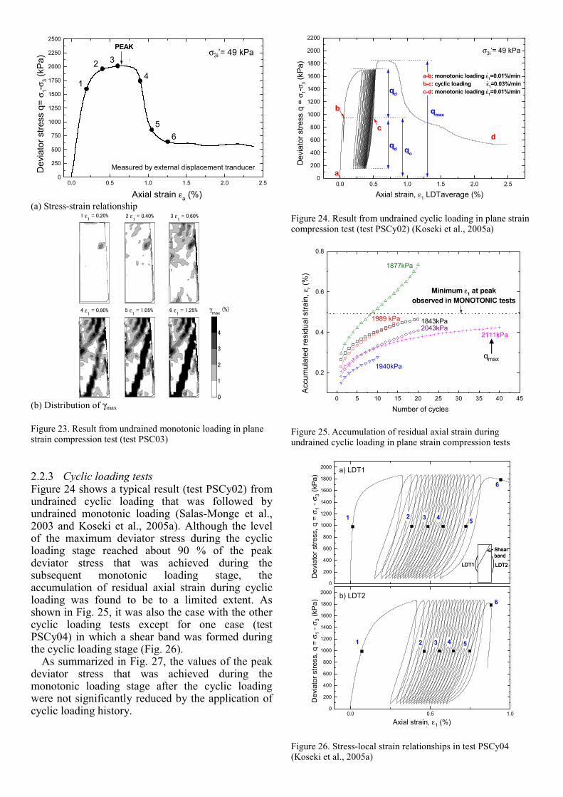
2.2.2 Monotonic loading tests Figure 20 shows a result from monotonic loading (test PSC05) conducted under undrained condition with an initial confining stress σ3i’ at 49 kPa (Salas-Monge et al., 2003). In general, the following behaviour was observed: 1) During the pre-peak phase, deformation was

uniform and no evident strain localization seemed to have taken place.

2) As the stress level approaches the peak stress state, strain started to accumulate at different defined regions within the specimen, and several “candidate” shear bands started to appear simultaneously.

3) After the peak stress state while sustaining the peak stress level, accumulation continued to take place in all of these prospective shear bands but was very low or null outside these regions.

4) Finally, during the post-peak phase, strain accumulation was limited to one (or two in some tests) of the “candidate” shear bands and continued until it was fully developed during residual state.

It should be noted that, during the post-peak phase, the zones outside these shear bands not only stopped accumulating strains but also experienced a certain degree of elastic rebound (i.e., negative ∆γmax in Fig. 20 (c) ). As shown in Fig. 21, the strain localization phenomenon could also be observed by comparing axial strains ε1 measured with vertical local

σ1 ε1

σ3

ε3σ2 ε2 = 0

Shear band

8cm6cm

16cm

σ1 ε1

σ3

ε3σ2 ε2 = 0

Shear band

σ1 ε1

σ3

ε3σ2 ε2 = 0

Shear bandShear band

8cm6cm

16cm

8cm6cm

16cm

Figure 17. Prismatic specimen for plane strain compression tests (Salas-Monge and Koseki, 2002)

Confining plate

End plate

Load cell

Slidingplate

Rollerbearings

Stiffening steelframe

Transparent plexiglassplate

Load cell

Horizontal LocalDeformation

Transducers (LDT)

Vertical LocalDeformation

Transducers (LDT)Proximeter and

target

Figure 18. Apparatus for plane strain compression tests (Salas-Monge and Koseki, 2002)

Figure 19. Digital photograph of specimen’s σ2 face taken during plane strain compression test

deformation transducers (LDTs, Goto et al., 1991) located across and outside the shear band and lateral strains ε3 measured in zones inside and outside the shear band by pairs of proximeter transducers.

Note also that, a crack could be observed after the test in the region where the local value of γmax exceeded 10 %, while the strain accumulation stopped during the post-peak phase (Fig. 22).

Figure 23 shows another example (test PSC03) of undrained monotonic loading test results. In this case, the stress-strain relationship around the peak stress state was relatively flat, as compared to the previous example (test PSC05, see Fig. 20). This behavior may be associated with formation of multiple shear bands around the peak stress state, which turned into formation of single full shear band in the post-peak phase, as can be seen from the local strain distributions. In both tests PSC03 (Fig. 23) and PSC05 (Fig. 20), the peak deviator stress was about 2000 kPa, on which no significant effect of the different patterns of the shear band development was observed.

0200400600800

10001200140016001800200022002400

0.0 0.5 1.0 1.5 2.0

PEAK PSC05

Axial strain ε1 (%) [External average]

Dev

iato

r stre

ss q

(kPa

)

σ3i’= 49 kPa

1

2 3

45

6

(a) Stress-strain relationship 1 ε

1 = 0.40% 2 ε

1 = 0.65% 3 ε

1 = 0.90%

4 ε1 = 1.15% 5 ε

1 = 1.40% 6 ε

1 = 1.75% γ

max (%)

0

1

2

3

4

(b) Distribution of γmax

Initial -> 1ε1 = 0.00 - 0.40%

1 -> 2ε1 = 0.40 - 0.65%

2 -> 3ε1 = 0.65 - 0.90%

3 -> 4ε1 = 0.90 - 1.15%

4 -> 5ε1 = 1.15 - 1.40%

5 -> 6 ε1

= 1.40 - 1.75% ∆γmax

(%)

0.0

0.5

1.0

(c) Distribution of ∆γmax Figure 20. Result from undrained monotonic loading in plane strain compression test (test PSC05) (Koseki et al., 2005a)

0

200

400

600

800

1000

1200

1400

1600

1800

2000

2200

0.0 0.5 1.0 1.5 2.0 2.5

Shear bands

LDT2LDT1

LDT1 LDT2

Axial strain ε1 (%)

Dev

iato

r stre

ss q

(kPa

)

0

200

400

600

800

1000

1200

1400

1600

1800

2000

2200

2400

-2.5 -2.0 -1.5 -1.0 -0.5 0.0

Bottom gap

Top gap

Shear bands

Bottom gap sensors Top gap sensors

Lateral strain ε3 (%)

Dev

iato

r stre

ss q

(kP

a)

Figure 21. Stress-local strain relationships in test PSC05

Fully developed shear band Crack

Figure 22. Condition of specimen after test PSC05

2.2.3 Cyclic loading tests Figure 24 shows a typical result (test PSCy02) from undrained cyclic loading that was followed by undrained monotonic loading (Salas-Monge et al., 2003 and Koseki et al., 2005a). Although the level of the maximum deviator stress during the cyclic loading stage reached about 90 % of the peak deviator stress that was achieved during the subsequent monotonic loading stage, the accumulation of residual axial strain during cyclic loading was found to be to a limited extent. As shown in Fig. 25, it was also the case with the other cyclic loading tests except for one case (test PSCy04) in which a shear band was formed during the cyclic loading stage (Fig. 26).

As summarized in Fig. 27, the values of the peak deviator stress that was achieved during the monotonic loading stage after the cyclic loading were not significantly reduced by the application of cyclic loading history.

0

250

500

750

1000

1250

1500

1750

2000

2250

2500

0.0 0.5 1.0 1.5 2.0 2.5

7

PEAK

6

543

2

1

Measured by external displacement tranducer

Axial strain εa (%)

Dev

iato

r stre

ss q

= σ 1-σ

3 (kP

a)σ3i’= 49 kPa

1

2 3

4

56

(a) Stress-strain relationship

5 ε1 = 1.05% 6 ε

1 = 1.25% 4 ε

1 = 0.90%

3 ε1 = 0.60%2 ε

1 = 0.40%1 ε

1 = 0.20%

γmax

(%)

0

1

2

3

4

(b) Distribution of γmax Figure 23. Result from undrained monotonic loading in plane strain compression test (test PSC03)

0

200

400

600

800

1000

1200

1400

1600

1800

2000

2200

0.0 0.5 1.0 1.5 2.0 2.5

c

b

a

d

qmax

qoqd

qd

Axial strain, ε1 LDTaverage (%)

Dev

iato

r stre

ss q

= σ

1-σ3 (

kPa)

a-b: monotonic loading ε1=0.01%/minb-c: cyclic loading ε1=0.03%/minc-d: monotonic loading ε1=0.01%/min

.

.

.

σ3i’= 49 kPa

Figure 24. Result from undrained cyclic loading in plane strain compression test (test PSCy02) (Koseki et al., 2005a)

0 5 10 15 20 25 30 35 40 45

0.2

0.4

0.6

0.8

2111kPa2043kPa

1940kPa

1877kPa

1989 kPa 1843kPa

Minimum ε1 at peakobserved in MONOTONIC tests

Acc

umul

ated

resi

dual

stra

in, ε

r (%

)

Number of cycles

qmax

Figure 25. Accumulation of residual axial strain during undrained cyclic loading in plane strain compression tests

0

200

400

600

800

1000

1200

1400

1600

1800

2000

6

54321

a) LDT1

Dev

iato

r stre

ss, q

= σ 1-σ

3 (kP

a)

0

200

400

600

800

1000

1200

1400

1600

1800

2000

0.0 0.5 1.0

6

54321

b) LDT2

Axial strain, ε1 (%) LDT2

Dev

iato

r stre

ss, q

= σ 1-σ

3 (kP

a)

a) LDT1

b) LDT2

LDT2LDT1

Shear band

LDT2LDT1

Shear band

Axial strain, ε1 (%)

Dev

iato

r stre

ss, q

= σ

1-σ

3(k

Pa)

Dev

iato

r stre

ss, q

= σ

1-σ

3(k

Pa)

Figure 26. Stress-local strain relationships in test PSCy04 (Koseki et al., 2005a)

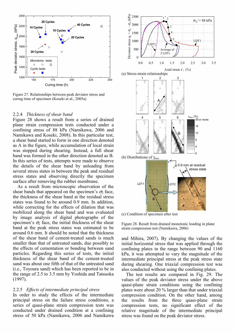
2.2.4 Thickness of shear band Figure 28 shows a result from a series of drained plane strain compression tests conducted under a confining stress of 88 kPa (Namikawa, 2006 and Namikawa and Koseki, 2008). In this particular test, a shear band started to form in one direction denoted as A in the figure, while accumulation of local strain was stopped during shearing. Instead, a full shear band was formed in the other direction denoted as B. In this series of tests, attempts were made to observe the details of the shear band by unloading from several stress states in between the peak and residual stress states and observing directly the specimen surface after removing the rubber membrane.

As a result from microscopic observation of the shear bands that appeared on the specimen’s σ2 face, the thickness of the shear band at the residual stress states was found to be around 0.9 mm. In addition, while correcting for the effects of dilation that was mobilized along the shear band and was evaluated by image analysis of digital photographs of the specimen’s σ2 face, the initial thickness of the shear band at the peak stress states was estimated to be around 0.6 mm. It should be noted that the thickness of the shear band of cement-treated sands is much smaller than that of untreated sands, due possibly to the effects of cementation or bonding between sand particles. Regarding this series of tests, the initial thickness of the shear band of the cement-treated sand was about one fifth of that of the untreated sand (i.e., Toyoura sand) which has been reported to be in the range of 2.5 to 3.5 mm by Yoshida and Tatsuoka (1997).

2.2.5 Effects of intermediate principal stress In order to study the effects of the intermediate principal stress on the failure stress conditions, a series of quasi-plane strain compression tests was conducted under drained condition at a confining stress of 50 kPa (Namikawa, 2006 and Namikawa

and Mihira, 2007). By changing the values of the initial horizontal stress that was applied through the confining plates in the range between 90 and 1160 kPa, it was attempted to vary the magnitude of the intermediate principal stress at the peak stress state during shearing. One triaxial compression test was also conducted without using the confining plates.

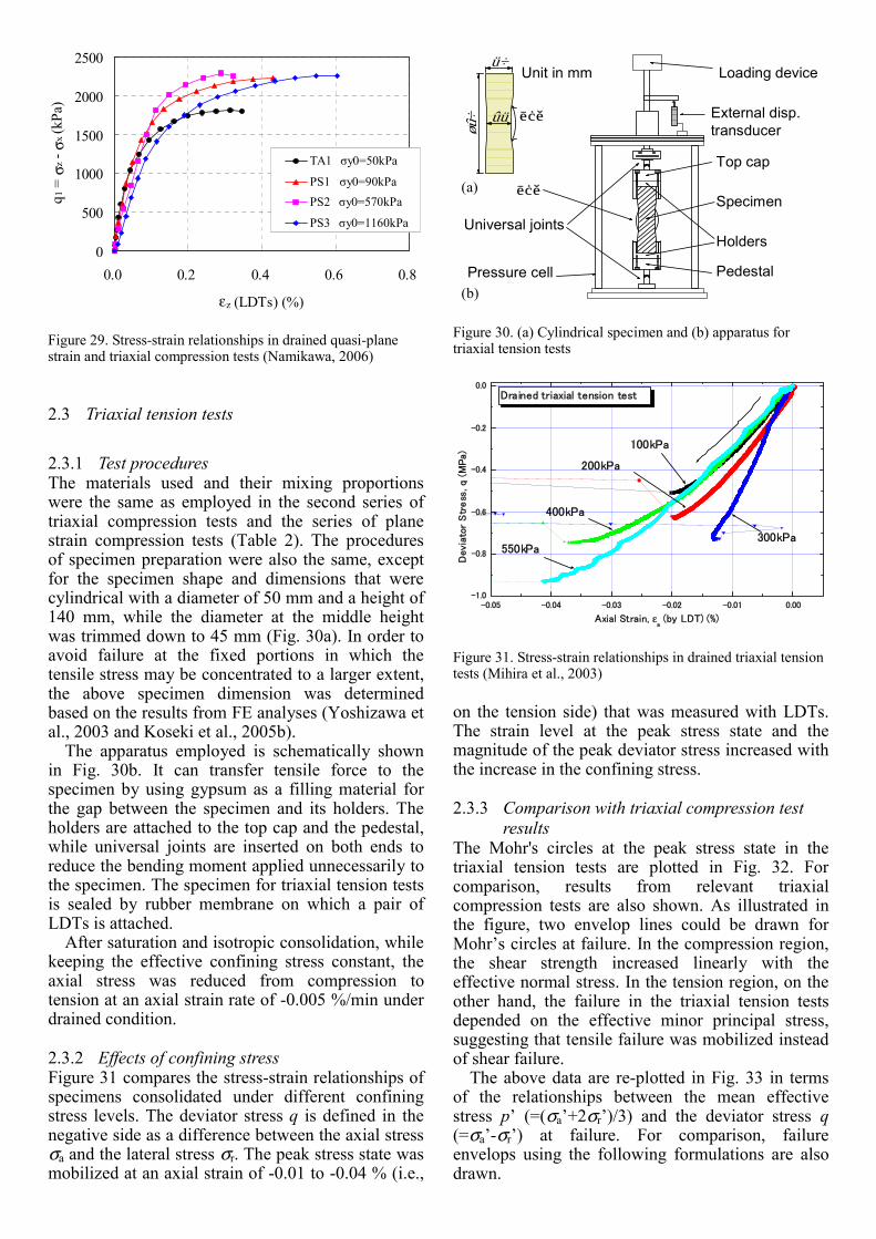
The test results are compared in Fig. 29. The values of the peak deviator stress under the above quasi-plane strain conditions using the confining plates were about 20 % larger than that under triaxial compression condition. On the other hand, among the results from the three quasi-plane strain compression tests, no significant effect of the relative magnitude of the intermediate principal stress was found on the peak deviator stress.

150 175 200 225 2501200

1400

1600

1800

2000

2200

2400

14 Cycles

20 Cycles

20 Cycles

20 Cycles

Monotonic tests

Cyclic tests

10 Cycles

40 Cycles

Pea

k de

viat

or s

tress

, qm

ax (k

Pa)

Curing time (h) Figure 27. Relationships between peak deviator stress and curing time of specimen (Koseki et al., 2005a)

0

500

1000

1500

2000

2500

0.0 0.5 1.0 1.5 2.0 2.5 3.0 3.5

Axial strain ε z (%)

σ3i’= 88 kPa1 2

3

4

56 LDT1

LDT2

Average of 2 LDTs

Dev

iato

r stre

ss q

1=

σ z–

σ x(k

Pa)

(a) Stress-strain relationships

0

4

8

12

16

20 or moreγmax (%)

A

B

1 2 3

4 5 6

(b) Distributions of γmax

LDT1 LDT2

z

x

B

0.9 mm at residual stress state

(c) Condition of specimen after test Figure 28. Result from drained monotonic loading in plane strain compression test (Namikawa, 2006)

2.3 Triaxial tension tests

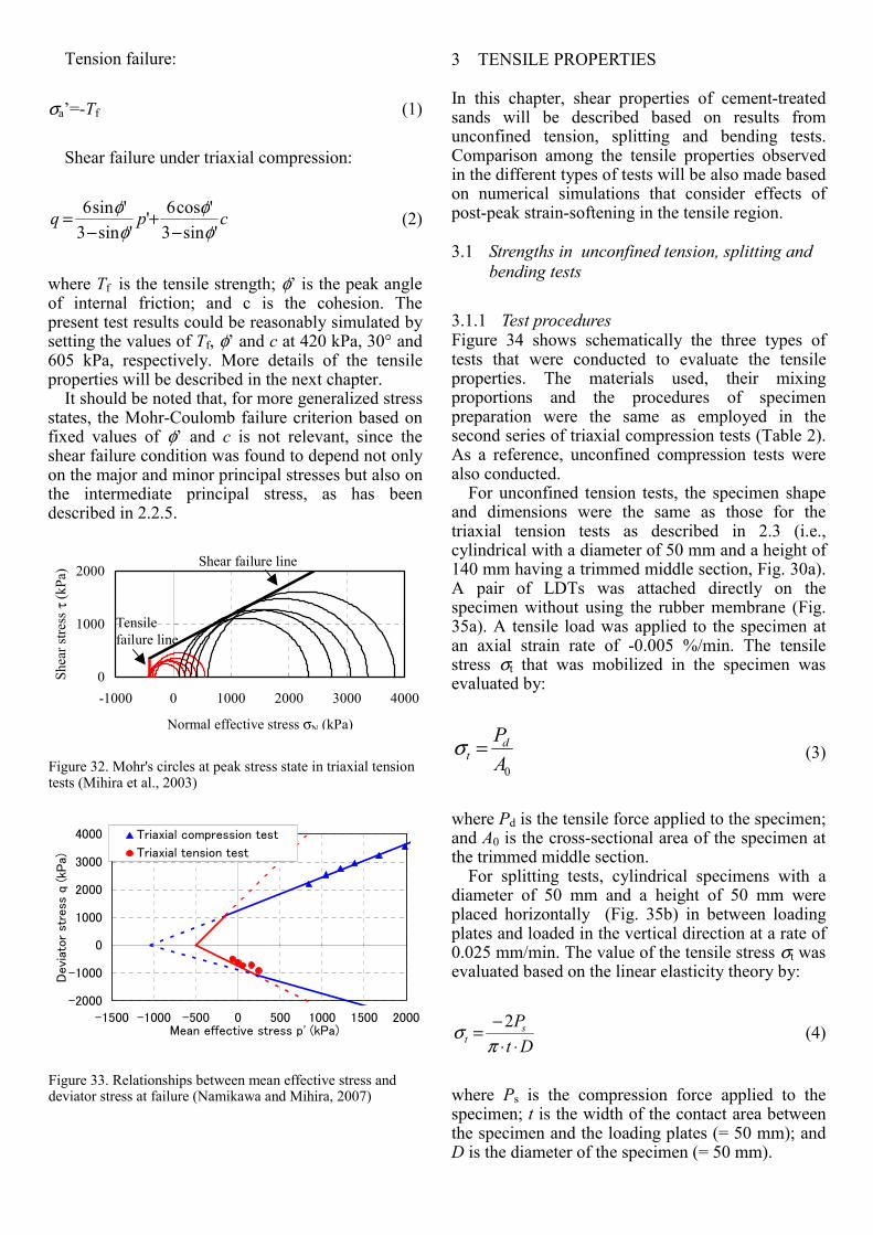
2.3.1 Test procedures The materials used and their mixing proportions were the same as employed in the second series of triaxial compression tests and the series of plane strain compression tests (Table 2). The procedures of specimen preparation were also the same, except for the specimen shape and dimensions that were cylindrical with a diameter of 50 mm and a height of 140 mm, while the diameter at the middle height was trimmed down to 45 mm (Fig. 30a). In order to avoid failure at the fixed portions in which the tensile stress may be concentrated to a larger extent, the above specimen dimension was determined based on the results from FE analyses (Yoshizawa et al., 2003 and Koseki et al., 2005b).

The apparatus employed is schematically shown in Fig. 30b. It can transfer tensile force to the specimen by using gypsum as a filling material for the gap between the specimen and its holders. The holders are attached to the top cap and the pedestal, while universal joints are inserted on both ends to reduce the bending moment applied unnecessarily to the specimen. The specimen for triaxial tension tests is sealed by rubber membrane on which a pair of LDTs is attached.

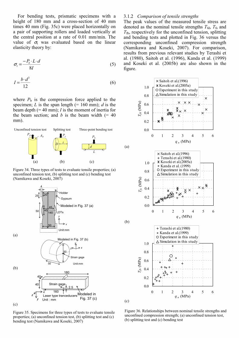
After saturation and isotropic consolidation, while keeping the effective confining stress constant, the axial stress was reduced from compression to tension at an axial strain rate of -0.005 %/min under drained condition.

2.3.2 Effects of confining stress Figure 31 compares the stress-strain relationships of specimens consolidated under different confining stress levels. The deviator stress q is defined in the negative side as a difference between the axial stress σa and the lateral stress σr. The peak stress state was mobilized at an axial strain of -0.01 to -0.04 % (i.e.,

on the tension side) that was measured with LDTs. The strain level at the peak stress state and the magnitude of the peak deviator stress increased with the increase in the confining stress.

2.3.3 Comparison with triaxial compression test results

The Mohr's circles at the peak stress state in the triaxial tension tests are plotted in Fig. 32. For comparison, results from relevant triaxial compression tests are also shown. As illustrated in the figure, two envelop lines could be drawn for Mohr’s circles at failure. In the compression region, the shear strength increased linearly with the effective normal stress. In the tension region, on the other hand, the failure in the triaxial tension tests depended on the effective minor principal stress, suggesting that tensile failure was mobilized instead of shear failure.

The above data are re-plotted in Fig. 33 in terms of the relationships between the mean effective stress p’ (=(σa’+2σr’)/3) and the deviator stress q (=σa’-σr’) at failure. For comparison, failure envelops using the following formulations are also drawn.

0

500

1000

1500

2000

2500

0.0 0.2 0.4 0.6 0.8

εz (LDTs) (%)

q 1 =

σz -

σx (

kPa)

TA1　σy0=50kPa

PS1 σy0=90kPaPS2　σy0=570kPa

PS3　σy0=1160kPa

Figure 29. Stress-strain relationships in drained quasi-plane strain and triaxial compression tests (Namikawa, 2006)

載荷装置

供試体

ペデスタル

外部変位計

ユニバーサル

ジョイント

三軸セル

LDT

キャップ

固定ホルダー

供試体の寸法と

LDTの設置位置

50

140 45 LDT

Unit in mm Loading device

External disp. transducer

Top cap

Specimen

Holders

PedestalPressure cell

Universal joints

(a)

(b) Figure 30. (a) Cylindrical specimen and (b) apparatus for triaxial tension tests

-0.05 -0.04 -0.03 -0.02 -0.01 0.00-1.0

-0.8

-0.6

-0.4

-0.2

0.0

200kPa

300kPa

400kPa

550kPa

100kPa

Drained triaxial tension test

Devia

tor

Str

ess

, q (

MPa)

Axial Strain, εa (by LDT) (%)

Figure 31. Stress-strain relationships in drained triaxial tension tests (Mihira et al., 2003)

Tension failure:

σa’=-Tf (1)

Shear failure under triaxial compression:

cpq'sin3

'cos6''sin3

'sin6φ

φφ

φ−

+−

= (2)

where Tf is the tensile strength; φ’ is the peak angle of internal friction; and c is the cohesion. The present test results could be reasonably simulated by setting the values of Tf, φ’ and c at 420 kPa, 30° and 605 kPa, respectively. More details of the tensile properties will be described in the next chapter.

It should be noted that, for more generalized stress states, the Mohr-Coulomb failure criterion based on fixed values of φ’ and c is not relevant, since the shear failure condition was found to depend not only on the major and minor principal stresses but also on the intermediate principal stress, as has been described in 2.2.5.

3 TENSILE PROPERTIES

In this chapter, shear properties of cement-treated sands will be described based on results from unconfined tension, splitting and bending tests. Comparison among the tensile properties observed in the different types of tests will be also made based on numerical simulations that consider effects of post-peak strain-softening in the tensile region.

3.1 Strengths in unconfined tension, splitting and bending tests

3.1.1 Test procedures Figure 34 shows schematically the three types of tests that were conducted to evaluate the tensile properties. The materials used, their mixing proportions and the procedures of specimen preparation were the same as employed in the second series of triaxial compression tests (Table 2). As a reference, unconfined compression tests were also conducted.

For unconfined tension tests, the specimen shape and dimensions were the same as those for the triaxial tension tests as described in 2.3 (i.e., cylindrical with a diameter of 50 mm and a height of 140 mm having a trimmed middle section, Fig. 30a). A pair of LDTs was attached directly on the specimen without using the rubber membrane (Fig. 35a). A tensile load was applied to the specimen at an axial strain rate of -0.005 %/min. The tensile stress σt that was mobilized in the specimen was evaluated by:

0APd

t =σ (3)

where Pd is the tensile force applied to the specimen; and A0 is the cross-sectional area of the specimen at the trimmed middle section.

For splitting tests, cylindrical specimens with a diameter of 50 mm and a height of 50 mm were placed horizontally (Fig. 35b) in between loading plates and loaded in the vertical direction at a rate of 0.025 mm/min. The value of the tensile stress σt was evaluated based on the linear elasticity theory by:

DtPs

t ⋅⋅−=

πσ 2

(4)

where Ps is the compression force applied to the specimen; t is the width of the contact area between the specimen and the loading plates (= 50 mm); and D is the diameter of the specimen (= 50 mm).

0

1000

2000

-1000 0 1000 2000 3000 4000

Normal effective stress σN (kPa)

Shea

r stre

ss τ

(kPa

) Shear failure line

Tensile failure line

Figure 32. Mohr's circles at peak stress state in triaxial tension tests (Mihira et al., 2003)

-2000

-1000

0

1000

2000

3000

4000

-1500 -1000 -500 0 500 1000 1500 2000Mean effective stress p' (kPa)

Dev

iato

r st

ress

q (kP

a)

Triaxial compression test

Triaxial tension test

Figure 33. Relationships between mean effective stress and deviator stress at failure (Namikawa and Mihira, 2007)

For bending tests, prismatic specimens with a height of 180 mm and a cross-section of 40 mm times 40 mm (Fig. 35c) were placed horizontally on a pair of supporting rollers and loaded vertically at the central position at a rate of 0.01 mm/min. The value of σt was evaluated based on the linear elasticity theory by:

IdLPb

t 8⋅⋅−=σ (5)

12

3dbI ⋅= (6)

where Pb is the compression force applied to the specimen; L is the span length (= 160 mm); d is the beam depth (= 40 mm); I is the moment of inertia for the beam section; and b is the beam width (= 40 mm).

3.1.2 Comparison of tensile strengths The peak values of the measured tensile stress are denoted as the nominal tensile strengths Tfd, Tfs and Tfb, respectively for the unconfined tension, splitting and bending tests and plotted in Fig. 36 versus the corresponding unconfined compression strength (Namikawa and Koseki, 2007). For comparison, results from previous relevant studies by Terashi et al. (1980), Saitoh et al. (1996), Kanda et al. (1999) and Koseki et al. (2005b) are also shown in the figure.

PsPd Pb

Unconfined tension test Splitting test Three-point bending test

A0

tDd

L

(a) (b) (c) Figure 34. Three types of tests to evaluate tensile properties; (a) unconfined tension test, (b) splitting test and (c) bending test (Namikawa and Koseki, 2007)

50

45

14050 LDTs45

x

y

Unit:mm

Gypsum

4

20

Modeled in Fig. 37 (a)

Holder25

(a)

50

50

x

y

z

Strain gage

Modeled in Fig. 37 (b)

Unit:mm (b)

Laser type tranceducers

180

40

40

160x

yz

2.5Strain gage

Unit : mm

Modeled in Fig. 37 (c)

(c) Figure 35. Specimens for three types of tests to evaluate tensile properties; (a) unconfined tension test, (b) splitting test and (c) bending test (Namikawa and Koseki, 2007)

0.0

0.2

0.4

0.6

0.8

1.0

0 1 2 3 4 5 6q u (MPa)

T fd (M

Pa)

Saitoh et al.(1996)Koseki et al.(2005a)Experiment in this studySimulation in this study

(a)

0.0

0.2

0.4

0.6

0.8

1.0

0 1 2 3 4 5 6 q u (MPa)

T fs (

MPa

)

Saitoh et al.(1996)Terashi et al.(1980)Koseki et al.(2005a)Kanda et al. (1999)Experiment in this studySimulation in this study

(b)

0.0

0.2

0.4

0.6

0.8

1.0

0 1 2 3 4 5 6q u (MPa)

T fb (M

Pa)

Terashi et al.(1980)Kanda et al.(1999)Experiment in this studySimulation in this study

(c) Figure 36. Relationships between nominal tensile strengths and unconfined compression strength; (a) unconfined tension test, (b) splitting test and (c) bending test

The nominal tensile strengths evaluated in the present study were consistent with the results from relevant studies and were larger in the order of the bending test, the unconfined tension test and the splitting test (i.e., Tfb>Tfd>Tfs).

In the next section, therefore, attempts were made to investigate into the discrepancy in the tensile strength properties that depend on the type of the tests employed. It should be noted that possible effect of anisotropy on the tensile strength properties is not considered herein, since it was found insignificant based on a series of unconfined tension and splitting tests by Koseki et al. (2009).

3.2 Numerical simulation of different types of tests

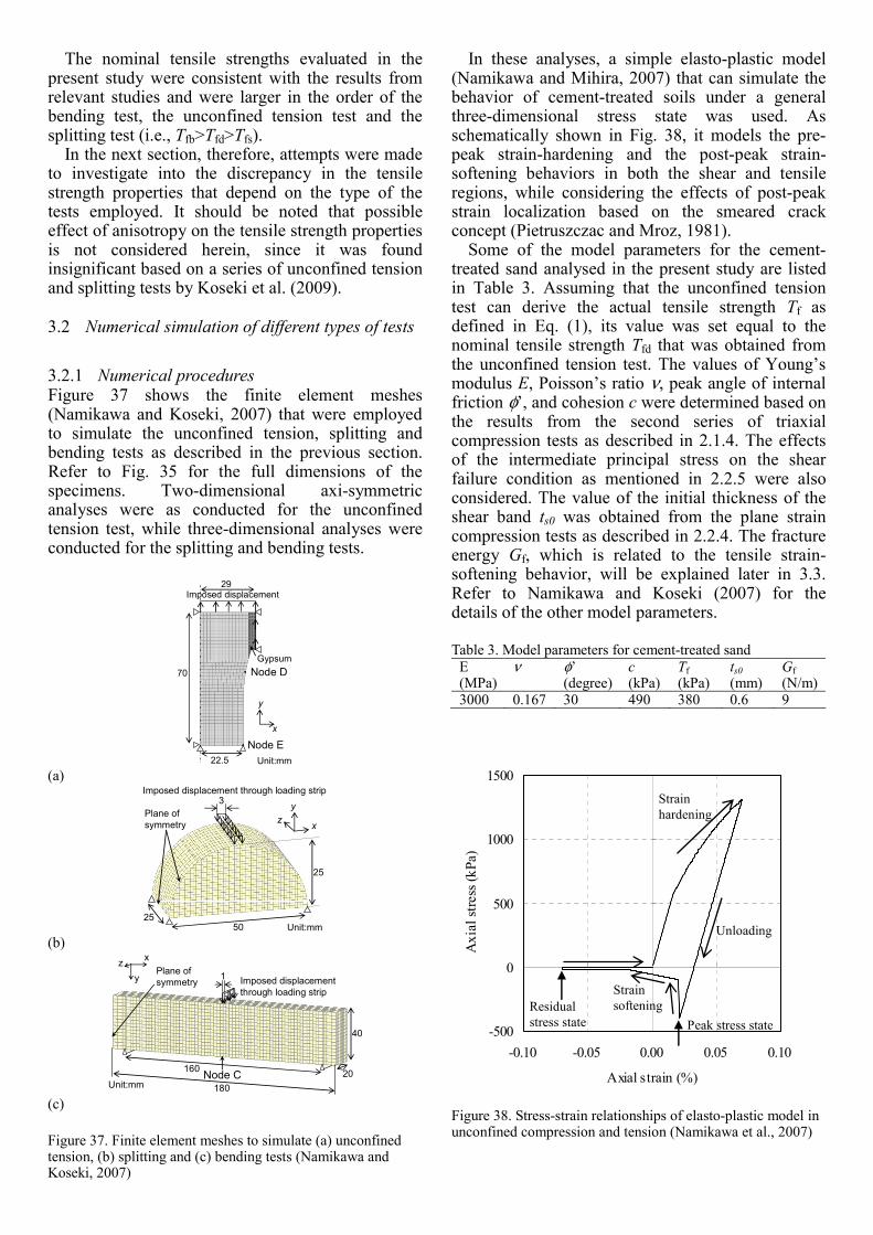
3.2.1 Numerical procedures Figure 37 shows the finite element meshes (Namikawa and Koseki, 2007) that were employed to simulate the unconfined tension, splitting and bending tests as described in the previous section. Refer to Fig. 35 for the full dimensions of the specimens. Two-dimensional axi-symmetric analyses were as conducted for the unconfined tension test, while three-dimensional analyses were conducted for the splitting and bending tests.

In these analyses, a simple elasto-plastic model (Namikawa and Mihira, 2007) that can simulate the behavior of cement-treated soils under a general three-dimensional stress state was used. As schematically shown in Fig. 38, it models the pre-peak strain-hardening and the post-peak strain-softening behaviors in both the shear and tensile regions, while considering the effects of post-peak strain localization based on the smeared crack concept (Pietruszczac and Mroz, 1981).

Some of the model parameters for the cement-treated sand analysed in the present study are listed in Table 3. Assuming that the unconfined tension test can derive the actual tensile strength Tf as defined in Eq. (1), its value was set equal to the nominal tensile strength Tfd that was obtained from the unconfined tension test. The values of Young’s modulus E, Poisson’s ratio ν, peak angle of internal friction φ’, and cohesion c were determined based on the results from the second series of triaxial compression tests as described in 2.1.4. The effects of the intermediate principal stress on the shear failure condition as mentioned in 2.2.5 were also considered. The value of the initial thickness of the shear band ts0 was obtained from the plane strain compression tests as described in 2.2.4. The fracture energy Gf, which is related to the tensile strain-softening behavior, will be explained later in 3.3. Refer to Namikawa and Koseki (2007) for the details of the other model parameters. Table 3. Model parameters for cement-treated sand

E (MPa)

ν φ’ (degree)

c (kPa)

Tf (kPa)

ts0 (mm)

Gf (N/m)

3000 0.167 30 490 380 0.6 9

Gypsum

x

y

Imposed displacement

Unit:mm22.5

70

29

Node D

Node E

(a)

Imposed displacement through loading strip

x

yz

3

5025

25

Unit:mm

Plane of symmetry

(b)

Imposed displacement through loading strip

Plane of symmetry 1

Node C

x

yz

180

160 20

40

Unit:mm (c) Figure 37. Finite element meshes to simulate (a) unconfined tension, (b) splitting and (c) bending tests (Namikawa and Koseki, 2007)

-500

0

500

1000

1500

-0.10 -0.05 0.00 0.05 0.10

Axial strain (%)

Axi

al st

ress

(kPa

)

Strain hardening

Unloading

Peak stress stateResidual stress state

Strain softening

Figure 38. Stress-strain relationships of elasto-plastic model in unconfined compression and tension (Namikawa et al., 2007)

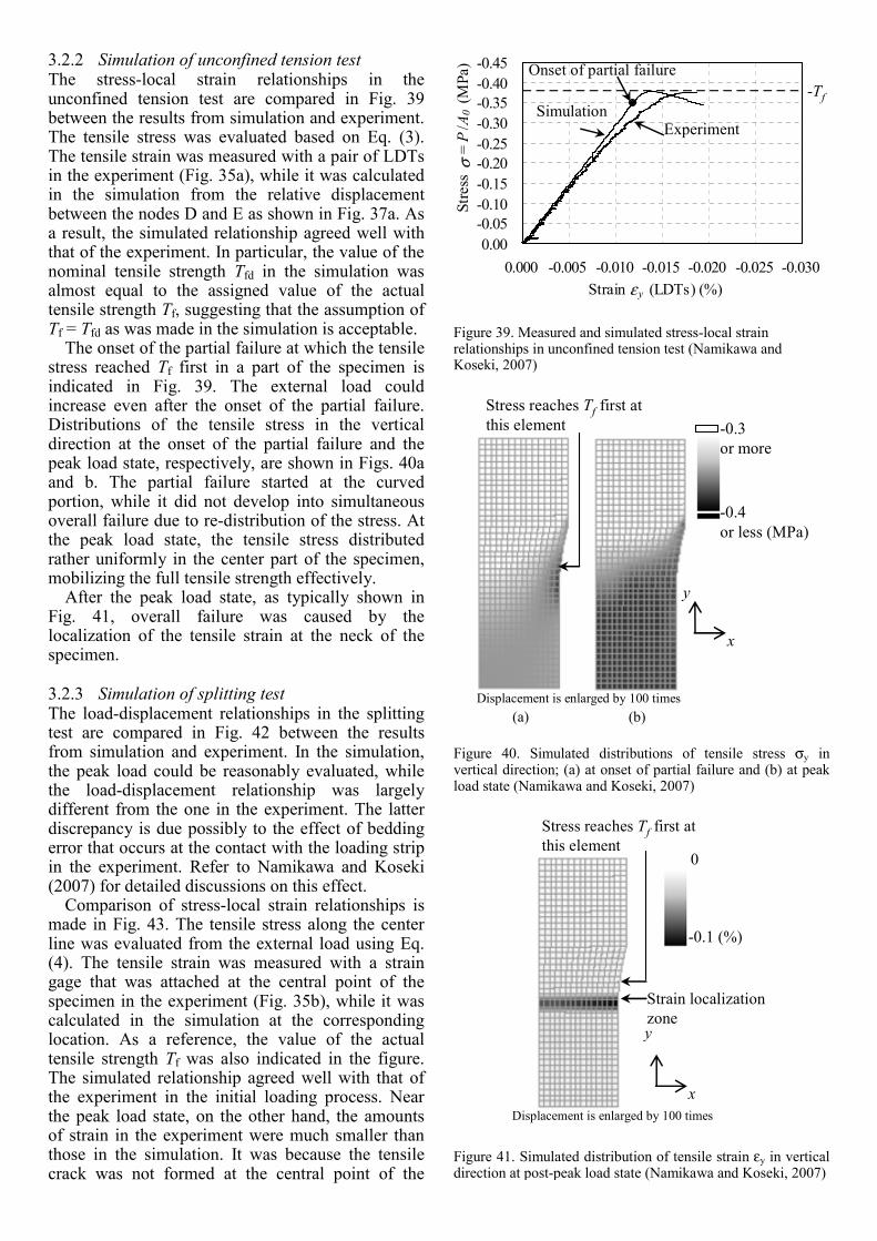
3.2.2 Simulation of unconfined tension test The stress-local strain relationships in the unconfined tension test are compared in Fig. 39 between the results from simulation and experiment. The tensile stress was evaluated based on Eq. (3). The tensile strain was measured with a pair of LDTs in the experiment (Fig. 35a), while it was calculated in the simulation from the relative displacement between the nodes D and E as shown in Fig. 37a. As a result, the simulated relationship agreed well with that of the experiment. In particular, the value of the nominal tensile strength Tfd in the simulation was almost equal to the assigned value of the actual tensile strength Tf, suggesting that the assumption of Tf = Tfd as was made in the simulation is acceptable.

The onset of the partial failure at which the tensile stress reached Tf first in a part of the specimen is indicated in Fig. 39. The external load could increase even after the onset of the partial failure. Distributions of the tensile stress in the vertical direction at the onset of the partial failure and the peak load state, respectively, are shown in Figs. 40a and b. The partial failure started at the curved portion, while it did not develop into simultaneous overall failure due to re-distribution of the stress. At the peak load state, the tensile stress distributed rather uniformly in the center part of the specimen, mobilizing the full tensile strength effectively.

After the peak load state, as typically shown in Fig. 41, overall failure was caused by the localization of the tensile strain at the neck of the specimen.

3.2.3 Simulation of splitting test The load-displacement relationships in the splitting test are compared in Fig. 42 between the results from simulation and experiment. In the simulation, the peak load could be reasonably evaluated, while the load-displacement relationship was largely different from the one in the experiment. The latter discrepancy is due possibly to the effect of bedding error that occurs at the contact with the loading strip in the experiment. Refer to Namikawa and Koseki (2007) for detailed discussions on this effect.

Comparison of stress-local strain relationships is made in Fig. 43. The tensile stress along the center line was evaluated from the external load using Eq. (4). The tensile strain was measured with a strain gage that was attached at the central point of the specimen in the experiment (Fig. 35b), while it was calculated in the simulation at the corresponding location. As a reference, the value of the actual tensile strength Tf was also indicated in the figure. The simulated relationship agreed well with that of the experiment in the initial loading process. Near the peak load state, on the other hand, the amounts of strain in the experiment were much smaller than those in the simulation. It was because the tensile crack was not formed at the central point of the

-0.45-0.40-0.35-0.30-0.25-0.20-0.15-0.10-0.050.00

-0.030-0.025-0.020-0.015-0.010-0.0050.000Strain ε y (LDTs) (%)

Stre

ss σ

= P

/A0

(MPa

)

ExperimentSimulation

-Tf

Onset of partial failure

Figure 39. Measured and simulated stress-local strain relationships in unconfined tension test (Namikawa and Koseki, 2007)

-0.3 or more

-0.4 or less (MPa)

x

y

Stress reaches Tf first at this element

Displacement is enlarged by 100 times (a) (b)

Figure 40. Simulated distributions of tensile stress σy in vertical direction; (a) at onset of partial failure and (b) at peak load state (Namikawa and Koseki, 2007)

0

-0.1 (%)

Stress reaches Tf first at this element

x

y

Strain localization zone

Displacement is enlarged by 100 times Figure 41. Simulated distribution of tensile strain εy in vertical direction at post-peak load state (Namikawa and Koseki, 2007)

0200

400600

8001000

12001400

0.0 0.2 0.4 0.6 0.8 1.0Axial displacement (mm)

Load

P (N

)

Simulation

Experiment

Peak load state to be analyzed in Fig. 44

Post-peak load state to be analyzed in Fig. 45

Figure 42. Measured and simulated load-displacement relationships in splitting test (Namikawa and Koseki, 2007)

-0.50

-0.40

-0.30

-0.20

-0.10

0.00-0.40-0.30-0.20-0.100.00

Strain ε x (％)

Stre

ss σ

2P

/ πrt

(MPa

)

SimulationExperiment

-Tf

-Tfs

Stre

ss σ

= -2

P / π

r t(

MPa

)

Figure 43. Measured and simulated stress-local strain relationships in splitting test (Namikawa and Koseki, 2007)

2.0 or more

0.0MPa

Plane of symmetry

Figure 44. Simulated distribution of deviator stress at peak load state (Namikawa and Koseki, 2007)

-1.3 %

0% or more

Plane of symmetry

Figure 45. Simulated distribution of tensile strain εx in horizontal direction at post-peak load state (Namikawa and Koseki, 2007)

specimen in the experiment, where the measurement with the strain gage was conducted.

Figure 44 shows the simulated distribution of the square root of the second invariant of deviator stress

at the peak load state. Large deviator stresses concentrated below the loading strip, which resulted into local shear failure. This would be the reason why the value of the nominal tensile strength Tfs in the splitting test was smaller than that of the actual tensile strength Tf as shown in Fig. 43. In addition, it was confirmed in the simulation that local tensile failure was also initiated at the peak load state along the center line of the specimen near its central part.

After the peak load state, as typically shown in Fig. 45, overall failure was caused by the localization of the tensile strain along the center line of the specimen.

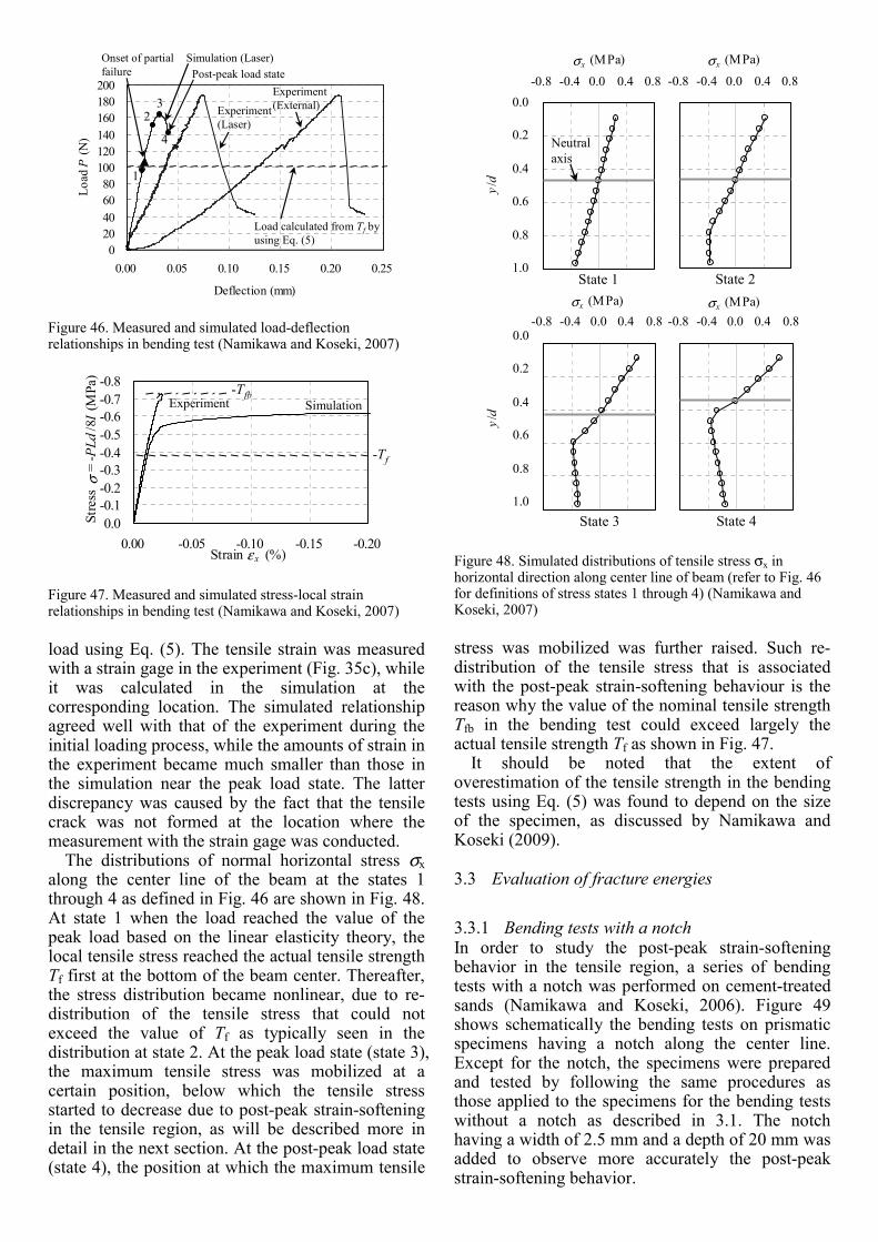
3.2.4 Simulation of bending test The load-deflection relationships in the bending test are compared in Fig. 46 between the results from simulation and experiment. In the experiment, two kinds of deflection data were measured with an external displacement transducer that was attached to the loading shaft and with a laser-type transducer that measured directly the deflection at the bottom of

the beam center, respectively. In the simulation, the vertical displacements at node C in Fig. 37c were employed as the deflection data, corresponding to the experimental data measured with the laser-type transducer. As a reference, the value of the peak load based on the linear elasticity theory that was evaluated using the actual tensile strength Tf as the tensile stress σt in Eq. (5) was also indicated in the figure.

It can be seen from Fig. 46 that the value of the peak load in the simulation was much larger than the one based on the linear elasticity theory, and it was rather close to the one observed in the experiment. However, the simulated load-deflection relationship was different from the one in the experiment based on the measurement with the laser-type transducer, due possibly to the effect of bedding error that occurs at the contact with the base support. It should be also noted that the load-deflection relationships based on the two types of displacement measurements in the experiment were significantly different from each other, due possibly to the effect of bedding error at the contact with the loading strip. Refer to Namikawa and Koseki (2007) for detailed discussions on these effects.

Comparison of stress-local strain relationships is made in Fig. 47. The tensile stress at the bottom of the beam center was evaluated from the external

sij

sijJ σσ212 =

020406080

100120140160180200

0.00 0.05 0.10 0.15 0.20 0.25

Deflection (mm)

Load

P (N

)Experiment (External)

Simulation (Laser)Onset of partial failure

1

23

4

Load calculated from Tf by using Eq. (5)

Experiment (Laser)

Post-peak load state

Figure 46. Measured and simulated load-deflection relationships in bending test (Namikawa and Koseki, 2007)

-0.8-0.7-0.6-0.5-0.4-0.3-0.2-0.10.0

-0.20-0.15-0.10-0.050.00Strain ε x (%)

Stre

ss σ

= -P

Ld/8

I (M

Pa)

SimulationExperiment

-Tf

-Tfb

Figure 47. Measured and simulated stress-local strain relationships in bending test (Namikawa and Koseki, 2007)

-0.8 -0.4 0.0 0.4 0.8σx (MPa)

-0.8 -0.4 0.0 0.4 0.8σx (MPa)

-0.8 -0.4 0.0 0.4 0.8σx (MPa)

0.0

0.2

0.4

0.6

0.8

1.0

-0.8 -0.4 0.0 0.4 0.8σx (MPa)

y/d

Neutral axis

State 1

0.0

0.2

0.4

0.6

0.8

1.0

-

y/d

State 2

State 3 State 4 Figure 48. Simulated distributions of tensile stress σx in horizontal direction along center line of beam (refer to Fig. 46 for definitions of stress states 1 through 4) (Namikawa and Koseki, 2007)

load using Eq. (5). The tensile strain was measured with a strain gage in the experiment (Fig. 35c), while it was calculated in the simulation at the corresponding location. The simulated relationship agreed well with that of the experiment during the initial loading process, while the amounts of strain in the experiment became much smaller than those in the simulation near the peak load state. The latter discrepancy was caused by the fact that the tensile crack was not formed at the location where the measurement with the strain gage was conducted.

The distributions of normal horizontal stress σx along the center line of the beam at the states 1 through 4 as defined in Fig. 46 are shown in Fig. 48. At state 1 when the load reached the value of the peak load based on the linear elasticity theory, the local tensile stress reached the actual tensile strength Tf first at the bottom of the beam center. Thereafter, the stress distribution became nonlinear, due to re-distribution of the tensile stress that could not exceed the value of Tf as typically seen in the distribution at state 2. At the peak load state (state 3), the maximum tensile stress was mobilized at a certain position, below which the tensile stress started to decrease due to post-peak strain-softening in the tensile region, as will be described more in detail in the next section. At the post-peak load state (state 4), the position at which the maximum tensile

stress was mobilized was further raised. Such re-distribution of the tensile stress that is associated with the post-peak strain-softening behaviour is the reason why the value of the nominal tensile strength Tfb in the bending test could exceed largely the actual tensile strength Tf as shown in Fig. 47.

It should be noted that the extent of overestimation of the tensile strength in the bending tests using Eq. (5) was found to depend on the size of the specimen, as discussed by Namikawa and Koseki (2009).

3.3 Evaluation of fracture energies

3.3.1 Bending tests with a notch In order to study the post-peak strain-softening behavior in the tensile region, a series of bending tests with a notch was performed on cement-treated sands (Namikawa and Koseki, 2006). Figure 49 shows schematically the bending tests on prismatic specimens having a notch along the center line. Except for the notch, the specimens were prepared and tested by following the same procedures as those applied to the specimens for the bending tests without a notch as described in 3.1. The notch having a width of 2.5 mm and a depth of 20 mm was added to observe more accurately the post-peak strain-softening behavior.

Load

Notch40 mm

160 mm

20 mm

Beam width: 40mm

2.5 mm

Figure 49. Notched prismatic specimen for bending test (Namikawa and Koseki, 2006) 0

5

10

15

20

25

30

35

40

0.0 0.2 0.4 0.6 0.8 1.0

δv　Laser　(mm)

Load

P　

(N)

BAb-1

BAb-2BAb-3

Figure 50. Load-deflection relationships in bending tests on notched specimen (Namikawa and Koseki, 2006)

P

δv

W0

W1 W2P0

δv0

Figure 51. Schematic figure on correction for effects of self weight of notched specimen (Namikawa and Koseki, 2006)

The load-deflection relationships of three identical specimens are shown in Fig. 50. After correcting for the effects of the self weight of the specimen as schematically shown in Fig. 51, the total amount of the fracture energy W that would be required to cause complete tensile failure can be evaluated as:

210 WWWW ++= (7)

where W0 is the area obtained from the measured load-deflection curve; W1 and W2 are the correction terms for the effects of the self weight of the specimen. It was assumed in the present study that W2 is approximately equal to W1, and the value of W1 can be evaluated as:

vovo mgPW δδ ⋅=⋅=21

01 (8)

where P0 is an equivalent load that would cause the same bending moment as the one caused by the self weight of the specimen; δvo is the deflection at which the specimen undergoes complete tensile failure; m is the mass of the specimen; and g is the gravitational acceleration. Then, the fracture energy Gf that is consumed per unit crack area is obtained as:

sf A

WG = (9)

where As is the fractured area.

As a result, the values of Gf as obtained from the three bending tests shown in Fig. 50 ranged from 9 to 12 N/m. In the FE analyses described in 3.2, therefore, the value of Gf for tensile fracture energy was set equal to 9 N/m (Table 3).

It should be noted that, since the pre-peak load-deflection curve was found to exhibit approximately linear elastic behavior, the above fracture energy can be regarded as the one that is consumed for plastic deformation during the post-peak strain-softening process. Thus, it was employed for modelling the

strain-softening behavior in the tensile region. Refer to Namikawa and Koseki (2006) for the details of the modelling.

3.3.2 Comparison between shear and tensile fracture energies

Based on the results from a series of plane strain compression tests as described in 2.2, the fracture energy Gfs that is consumed per unit area of shear band during its formation was evaluated to range from 100 to 180 N/m (Namikawa and Koseki, 2006).

The above values of the shear fracture energy were significantly larger than those of the tensile fracture energy as described in 3.3.1. This discrepancy may be explained by different mechanisms of shear and tensile failures. As typically shown in Fig. 52, formation of a line crack was observed during tensile failure, while formation of a shear band having a finite thickness was observed during shear failure as described in 2.2.4. Therefore, as schematically shown in Fig. 53, shear failure requires more energy to induce breakage of the cementation between particle contacts than tensile failure does.

0.5mmImmediately above the notch

Figure 52. Formation of line crack in bending test on notched specimen (Namikawa and Koseki, 2006)

Tensile stress Shear stress

Unit breakage area in shear failure

Unit breakage area in tensile failure

Thickness of shear band

Figure 53. Schematic figure on different microscopic failure modes in shear and tension (Namikawa and Koseki, 2006)

Lattice typeground improvement

Figure 54. Case history of application of lattice type ground improvement by in-situ cement-mixing for liquefaction mitigation (Namikawa et al, 2005)

Inertia forceDynamic earth

pressure

Inertia force

Liquefiable sand depositz

Improved soil grids

Figure 55. Schematic figure on external forces acting on improved soil walls during earthquake (Namikawa et al, 2007)

4 APPLICATION TO MITIGATION OF LIQUEFACTION-INDUCED DAMAGE

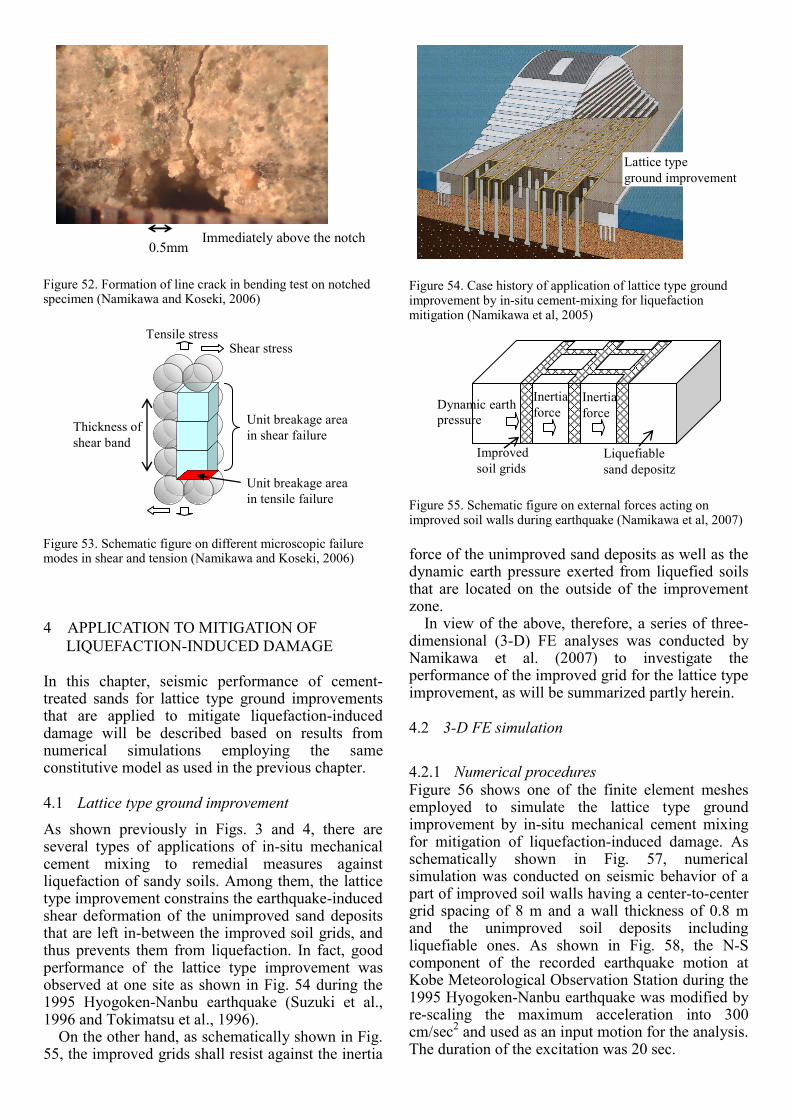
In this chapter, seismic performance of cement-treated sands for lattice type ground improvements that are applied to mitigate liquefaction-induced damage will be described based on results from numerical simulations employing the same constitutive model as used in the previous chapter.

4.1 Lattice type ground improvement

As shown previously in Figs. 3 and 4, there are several types of applications of in-situ mechanical cement mixing to remedial measures against liquefaction of sandy soils. Among them, the lattice type improvement constrains the earthquake-induced shear deformation of the unimproved sand deposits that are left in-between the improved soil grids, and thus prevents them from liquefaction. In fact, good performance of the lattice type improvement was observed at one site as shown in Fig. 54 during the 1995 Hyogoken-Nanbu earthquake (Suzuki et al., 1996 and Tokimatsu et al., 1996).

On the other hand, as schematically shown in Fig. 55, the improved grids shall resist against the inertia

force of the unimproved sand deposits as well as the dynamic earth pressure exerted from liquefied soils that are located on the outside of the improvement zone.

In view of the above, therefore, a series of three-dimensional (3-D) FE analyses was conducted by Namikawa et al. (2007) to investigate the performance of the improved grid for the lattice type improvement, as will be summarized partly herein.

4.2 3-D FE simulation

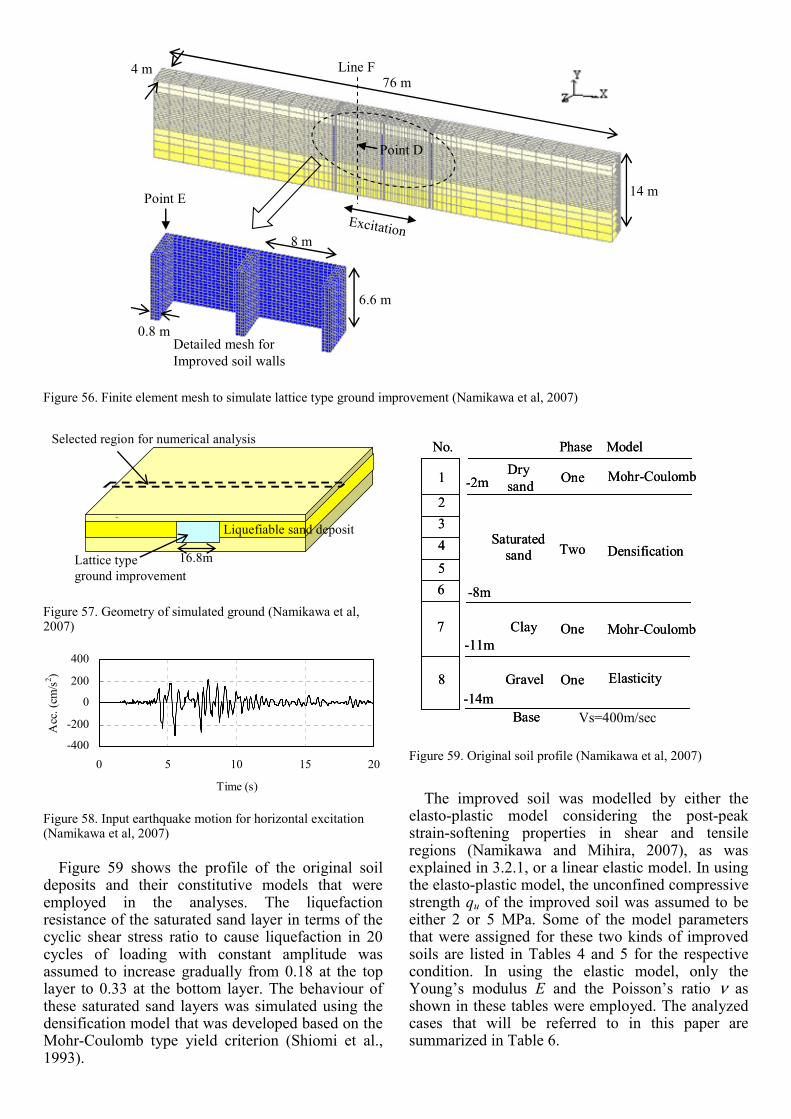
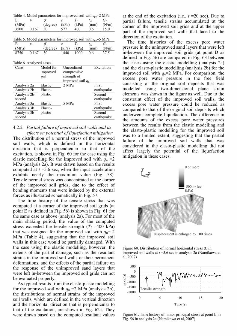
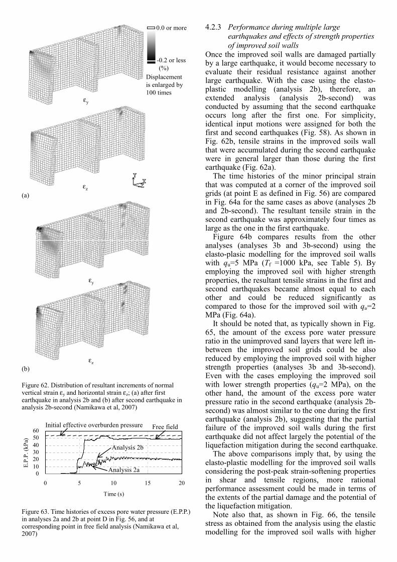
4.2.1 Numerical procedures Figure 56 shows one of the finite element meshes employed to simulate the lattice type ground improvement by in-situ mechanical cement mixing for mitigation of liquefaction-induced damage. As schematically shown in Fig. 57, numerical simulation was conducted on seismic behavior of a part of improved soil walls having a center-to-center grid spacing of 8 m and a wall thickness of 0.8 m and the unimproved soil deposits including liquefiable ones. As shown in Fig. 58, the N-S component of the recorded earthquake motion at Kobe Meteorological Observation Station during the 1995 Hyogoken-Nanbu earthquake was modified by re-scaling the maximum acceleration into 300 cm/sec2 and used as an input motion for the analysis. The duration of the excitation was 20 sec.

76 m4 m

6.6 m

Excitation

Point E

Point D

Line F

0.8 mDetailed mesh forImproved soil walls

14 m

8 m

Figure 56. Finite element mesh to simulate lattice type ground improvement (Namikawa et al, 2007)

▽ Liquefiable sand deposit

Selected region for numerical analysis

16.8mLattice typeground improvement

Figure 57. Geometry of simulated ground (Namikawa et al, 2007)

-400

-200

0

200

400

0 5 10 15 20

Time (s)

Acc

. (cm

/s2 )

Figure 58. Input earthquake motion for horizontal excitation (Namikawa et al, 2007)

Vs=400m/sec

1

23456

7

8

No. Phase Model

-2m

-8m

-11m

-14m

One Mohr-Coulomb

Densification

Mohr-Coulomb

Drysand

Saturatedsand

Clay

Gravel

Base

Two

One

One Elasticity

Vs=400m/sec

1

23456

7

8

No. Phase Model

-2m

-8m

-11m

-14m

One Mohr-Coulomb

Densification

Mohr-Coulomb

Drysand

Saturatedsand

Clay

Gravel

Base

Two

One

One Elasticity

Figure 59. Original soil profile (Namikawa et al, 2007)

Figure 59 shows the profile of the original soil

deposits and their constitutive models that were employed in the analyses. The liquefaction resistance of the saturated sand layer in terms of the cyclic shear stress ratio to cause liquefaction in 20 cycles of loading with constant amplitude was assumed to increase gradually from 0.18 at the top layer to 0.33 at the bottom layer. The behaviour of these saturated sand layers was simulated using the densification model that was developed based on the Mohr-Coulomb type yield criterion (Shiomi et al., 1993).

The improved soil was modelled by either the elasto-plastic model considering the post-peak strain-softening properties in shear and tensile regions (Namikawa and Mihira, 2007), as was explained in 3.2.1, or a linear elastic model. In using the elasto-plastic model, the unconfined compressive strength qu of the improved soil was assumed to be either 2 or 5 MPa. Some of the model parameters that were assigned for these two kinds of improved soils are listed in Tables 4 and 5 for the respective condition. In using the elastic model, only the Young’s modulus E and the Poisson’s ratio ν as shown in these tables were employed. The analyzed cases that will be referred to in this paper are summarized in Table 6.

-500 or less(kPa)

0 or more

Displacement is enlarged by 100 times

Figure 60. Distribution of normal horizontal stress σz in improved soil walls at t =5.6 sec in analysis 2a (Namikawa et al, 2007)

-2000-1500-1000-500

0500

0 5 10 15 20

Time (s)

σ 3 (k

Pa)

Tensile strength

Figure 61. Time history of minor principal stress at point E in Fig. 56 in analysis 2a (Namikawa et al, 2007)

Table 4. Model parameters for improved soil with qu=2 MPa E (MPa)

ν φ’ (degree)

c (kPa)

Tf (kPa)

ts0 (mm)

Gf (N/m)

3500 0.167 30 577 400 0.6 15.0 Table 5. Model parameters for improved soil with qu=5 MPa

E (MPa)

ν φ’ (degree)

c (kPa)

Tf (kPa)

ts0 (mm)

Gf (N/m)

8750 0.167 30 1440 1000 0.6 37.5 Table 6. Analyzed cases

Case Model for improved soil

Unconfined compressive strength of improved soil qu

Excitation

Analysis 2a Elastic Analysis 2b

First earthquake

Analysis 2b-second

Elasto-plastic

2 MPa

Second earthquake

Analysis 3a Elastic Analysis 3b

First earthquake

Analysis 3b-second

Elasto-plastic

5 MPa

Second earthquake

4.2.2 Partial failure of improved soil walls and its effects on potential of liquefaction mitigation

The distribution of a normal stress of the improved soil walls, which is defined in the horizontal direction that is perpendicular to that of the excitation, is shown in Fig. 60 for the case using the elastic modelling for the improved soil with qu =2 MPa (analysis 2a). It was drawn based on the results computed at t =5.6 sec, when the input acceleration exhibits nearly the maximum value (Fig. 58). Tensile normal stress was concentrated at the corner of the improved soil grids, due to the effect of bending moments that were induced by the external forces as illustrated schematically in Fig. 57.

The time history of the tensile stress that was computed at a corner of the improved soil grids (at point E as defined in Fig. 56) is shown in Fig. 61 for the same case as above (analysis 2a). For most of the main shaking period, the value of the computed stress exceeded the tensile strength (Tf =400 kPa) that was assigned for the improved soil with qu= 2 MPa (Table 4), suggesting that the improved soil walls in this case would be partially damaged. With the case using the elastic modelling, however, the extents of the partial damage, such as the resultant strains in the improved soil walls or their permanent deformations, and the effects of the partial failure on the response of the unimproved sand layers that were left in-between the improved soil grids can not be evaluated properly.

As typical results from the elasto-plasic modelling for the improved soil with qu =2 MPa (analysis 2b), the distributions of normal strains of the improved soil walls, which are defined in the vertical direction and the horizontal direction that is perpendicular to that of the excitation, are shown in Fig. 62a. They were drawn based on the computed resultant values

at the end of the excitation (i.e., t =20 sec). Due to partial failure, tensile strains accumulated at the corner of the improved soil grids and at the upper part of the improved soil walls that faced to the direction of the excitation.

The time histories of the excess pore water pressure in the unimproved sand layers that were left in-between the improved soil grids (at point D as defined in Fig. 56) are compared in Fig. 63 between the cases using the elastic modelling (analysis 2a) and the elasto-plastic modelling (analysis 2b) for the improved soil with qu=2 MPa. For comparison, the excess pore water pressure in the free field consisting of the original soil deposits that was modelled using two-dimensional plane strain elements was shown in the figure as well. Due to the constraint effect of the improved soil walls, the excess pore water pressure could be reduced as compared to that of the original soil deposits which underwent complete liquefaction. The difference in the amounts of the excess pore water pressures between the results from the elastic modelling and the elasto-plastic modelling for the improved soil was to a limited extent, suggesting that the partial failure of the improved soil walls that was considered in the elasto-plastic modelling did not affect largely the potential of the liquefaction mitigation in these cases.

εz

εy

-0.2 or less

0.0 or more

(%)Displacement is enlarged by 100 times

(a)

εz

εy

(b) Figure 62. Distribution of resultant increments of normal vertical strain εy and horizontal strain εz; (a) after first earthquake in analysis 2b and (b) after second earthquake in analysis 2b-second (Namikawa et al, 2007)

0102030405060

0 5 10 15 20

Time (s)

E.P.

P. (k

Pa)

Initial effective overburden pressure Free field

Analysis 2b

Analysis 2a

Figure 63. Time histories of excess pore water pressure (E.P.P.) in analyses 2a and 2b at point D in Fig. 56, and at corresponding point in free field analysis (Namikawa et al, 2007)

4.2.3 Performance during multiple large earthquakes and effects of strength properties of improved soil walls

Once the improved soil walls are damaged partially by a large earthquake, it would become necessary to evaluate their residual resistance against another large earthquake. With the case using the elasto-plastic modelling (analysis 2b), therefore, an extended analysis (analysis 2b-second) was conducted by assuming that the second earthquake occurs long after the first one. For simplicity, identical input motions were assigned for both the first and second earthquakes (Fig. 58). As shown in Fig. 62b, tensile strains in the improved soils wall that were accumulated during the second earthquake were in general larger than those during the first earthquake (Fig. 62a).

The time histories of the minor principal strain that was computed at a corner of the improved soil grids (at point E as defined in Fig. 56) are compared in Fig. 64a for the same cases as above (analyses 2b and 2b-second). The resultant tensile strain in the second earthquake was approximately four times as large as the one in the first earthquake.

Figure 64b compares results from the other analyses (analyses 3b and 3b-second) using the elasto-plasic modelling for the improved soil walls with qu=5 MPa (Tf =1000 kPa, see Table 5). By employing the improved soil with higher strength properties, the resultant tensile strains in the first and second earthquakes became almost equal to each other and could be reduced significantly as compared to those for the improved soil with qu=2 MPa (Fig. 64a).

It should be noted that, as typically shown in Fig. 65, the amount of the excess pore water pressure ratio in the unimproved sand layers that were left in-between the improved soil grids could be also reduced by employing the improved soil with higher strength properties (analyses 3b and 3b-second). Even with the cases employing the improved soil with lower strength properties (qu=2 MPa), on the other hand, the amount of the excess pore water pressure ratio in the second earthquake (analysis 2b-second) was almost similar to the one during the first earthquake (analysis 2b), suggesting that the partial failure of the improved soil walls during the first earthquake did not affect largely the potential of the liquefaction mitigation during the second earthquake.

The above comparisons imply that, by using the elasto-plastic modelling for the improved soil walls considering the post-peak strain-softening properties in shear and tensile regions, more rational performance assessment could be made in terms of the extents of the partial damage and the potential of the liquefaction mitigation.

Note also that, as shown in Fig. 66, the tensile stress as obtained from the analysis using the elastic modelling for the improved soil walls with higher

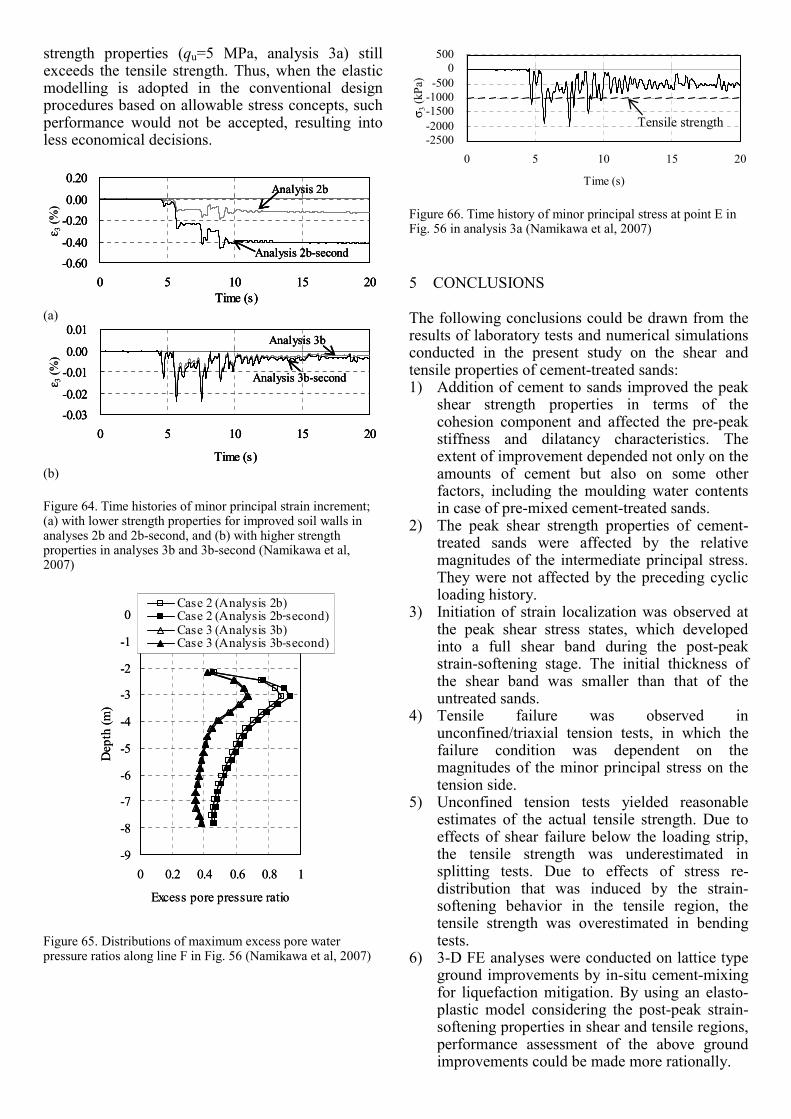
-0.60-0.40

-0.200.00

0.20

0 5 10 15 20Time (s)

Analysis 2b

Analysis 2b-second

ε 3(%

)

-0.60-0.40

-0.200.00

0.20

0 5 10 15 20Time (s)

Analysis 2b

Analysis 2b-second-0.60-0.40

-0.200.00

0.20

0 5 10 15 20Time (s)

Analysis 2b

Analysis 2b-second

ε 3(%

)

(a)

-0.03-0.02

-0.010.00

0.01

0 5 10 15 20

Time (s)

Analysis 3b

Analysis 3b-secondε 3(%

)

-0.03-0.02

-0.010.00

0.01

0 5 10 15 20

Time (s)

Analysis 3b

Analysis 3b-second

-0.03-0.02

-0.010.00

0.01

0 5 10 15 20

Time (s)

Analysis 3b

Analysis 3b-secondε 3(%

)

(b) Figure 64. Time histories of minor principal strain increment; (a) with lower strength properties for improved soil walls in analyses 2b and 2b-second, and (b) with higher strength properties in analyses 3b and 3b-second (Namikawa et al, 2007)

-9

-8

-7

-6

-5

-4

-3

-2

-1

0

0 0.2 0.4 0.6 0.8 1

Excess pore pressure ratio

Dep

th (m

)

Case 2 (Analysis 2b)Case 2 (Analysis 2b second)Case 3 (Analysis 3b)Case 3 (Analysis 3b second)

-

-

-9

-8

-7

-6

-5

-4

-3

-2

-1

0

0 0.2 0.4 0.6 0.8 1

Excess pore pressure ratio

Dep

th (m

)

Case 2 (Analysis 2b)Case 2 (Analysis 2b second)Case 3 (Analysis 3b)Case 3 (Analysis 3b second)

-

-

Figure 65. Distributions of maximum excess pore water pressure ratios along line F in Fig. 56 (Namikawa et al, 2007)

strength properties (qu=5 MPa, analysis 3a) still exceeds the tensile strength. Thus, when the elastic modelling is adopted in the conventional design procedures based on allowable stress concepts, such performance would not be accepted, resulting into less economical decisions.

5 CONCLUSIONS

The following conclusions could be drawn from the results of laboratory tests and numerical simulations conducted in the present study on the shear and tensile properties of cement-treated sands: 1) Addition of cement to sands improved the peak

shear strength properties in terms of the cohesion component and affected the pre-peak stiffness and dilatancy characteristics. The extent of improvement depended not only on the amounts of cement but also on some other factors, including the moulding water contents in case of pre-mixed cement-treated sands.

2) The peak shear strength properties of cement-treated sands were affected by the relative magnitudes of the intermediate principal stress. They were not affected by the preceding cyclic loading history.

3) Initiation of strain localization was observed at the peak shear stress states, which developed into a full shear band during the post-peak strain-softening stage. The initial thickness of the shear band was smaller than that of the untreated sands.

4) Tensile failure was observed in unconfined/triaxial tension tests, in which the failure condition was dependent on the magnitudes of the minor principal stress on the tension side.

5) Unconfined tension tests yielded reasonable estimates of the actual tensile strength. Due to effects of shear failure below the loading strip, the tensile strength was underestimated in splitting tests. Due to effects of stress re-distribution that was induced by the strain-softening behavior in the tensile region, the tensile strength was overestimated in bending tests.

6) 3-D FE analyses were conducted on lattice type ground improvements by in-situ cement-mixing for liquefaction mitigation. By using an elasto-plastic model considering the post-peak strain-softening properties in shear and tensile regions, performance assessment of the above ground improvements could be made more rationally.

-2500-2000-1500-1000

-5000

500

0 5 10 15 20

Time (s)

Tensile strengthσ 3(k

Pa)

Figure 66. Time history of minor principal stress at point E in Fig. 56 in analysis 3a (Namikawa et al, 2007)

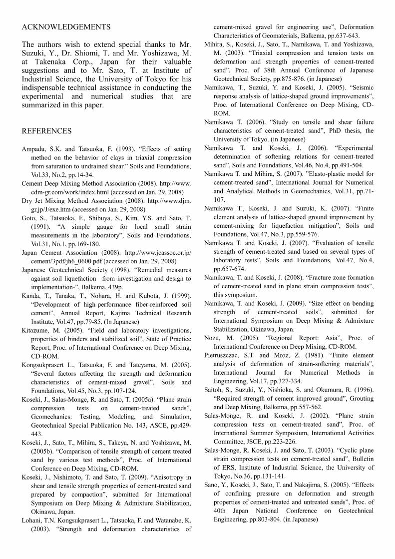
ACKNOWLEDGEMENTS

The authors wish to extend special thanks to Mr. Suzuki, Y., Dr. Shiomi, T. and Mr. Yoshizawa, M. at Takenaka Corp., Japan for their valuable suggestions and to Mr. Sato, T. at Institute of Industrial Science, the University of Tokyo for his indispensable technical assistance in conducting the experimental and numerical studies that are summarized in this paper.

REFERENCES

Ampadu, S.K. and Tatsuoka, F. (1993). “Effects of setting method on the behavior of clays in triaxial compression from saturation to undrained shear.” Soils and Foundations, Vol.33, No.2, pp.14-34.

Cement Deep Mixing Method Association (2008). http://www. cdm-gr.com/work/index.html (accessed on Jan. 29, 2008)

Dry Jet Mixing Method Association (2008). http://www.djm. gr.jp/J/exe.htm (accessed on Jan. 29, 2008)

Goto, S., Tatsuoka, F., Shibuya, S., Kim, Y.S. and Sato, T. (1991). “A simple gauge for local small strain measurements in the laboratory”, Soils and Foundations, Vol.31, No.1, pp.169-180.

Japan Cement Association (2008). http://www.jcassoc.or.jp/ cement/3pdf/jh6_0600.pdf (accessed on Jan. 29, 2008)

Japanese Geotechnical Society (1998). “Remedial measures against soil liquefaction –from investigation and design to implementation-”, Balkema, 439p.

Kanda, T., Tanaka, T., Nohara, H. and Kubota, J. (1999). “Development of high-performance fiber-reinforced soil cement”, Annual Report, Kajima Technical Research Institute, Vol.47, pp.79-85. (In Japanese)

Kitazume, M. (2005). “Field and laboratory investigations, properties of binders and stabilized soil”, State of Practice Report, Proc. of International Conference on Deep Mixing, CD-ROM.

Kongsukprasert L., Tatsuoka, F. and Tateyama, M. (2005). “Several factors affecting the strength and deformation characteristics of cement-mixed gravel”, Soils and Foundations, Vol.45, No.3, pp.107-124.

Koseki, J., Salas-Monge, R. and Sato, T. (2005a). “Plane strain compression tests on cement-treated sands”, Geomechanics: Testing, Modeling, and Simulation, Geotechnical Special Publication No. 143, ASCE, pp.429-443.

Koseki, J., Sato, T., Mihira, S., Takeya, N. and Yoshizawa, M. (2005b). “Comparison of tensile strength of cement treated sand by various test methods”, Proc. of International Conference on Deep Mixing, CD-ROM.

Koseki, J., Nishimoto, T. and Sato, T. (2009). “Anisotropy in shear and tensile strength properties of cement-treated sand prepared by compaction”, submitted for International Symposium on Deep Mixing & Admixture Stabilization, Okinawa, Japan.

Lohani, T.N. Kongsukprasert L., Tatsuoka, F. and Watanabe, K. (2003). “Strength and deformation characteristics of

cement-mixed gravel for engineering use”, Deformation Characteristics of Geomaterials, Balkema, pp.637-643.

Mihira, S., Koseki, J., Sato, T., Namikawa, T. and Yoshizawa, M. (2003). “Triaxial compression and tension tests on deformation and strength properties of cement-treated sand”. Proc. of 38th Annual Conference of Japanese Geotechnical Society, pp.875-876. (in Japanese)

Namikawa, T., Suzuki, Y. and Koseki, J. (2005). “Seismic response analysis of lattice-shaped ground improvements”, Proc. of International Conference on Deep Mixing, CD-ROM.

Namikawa T. (2006). “Study on tensile and shear failure characteristics of cement-treated sand”, PhD thesis, the University of Tokyo. (in Japanese)

Namikawa T. and Koseki, J. (2006). “Experimental determination of softening relations for cement-treated sand”, Soils and Foundations, Vol.46, No.4, pp.491-504.

Namikawa T. and Mihira, S. (2007). ”Elasto-plastic model for cement-treated sand”, International Journal for Numerical and Analytical Methods in Geomechanics, Vol.31, pp.71-107.

Namikawa T., Koseki, J. and Suzuki, K. (2007). “Finite element analysis of lattice-shaped ground improvement by cement-mixing for liquefaction mitigation”, Soils and Foundations, Vol.47, No.3, pp.559-576.

Namikawa T. and Koseki, J. (2007). “Evaluation of tensile strength of cement-treated sand based on several types of laboratory tests”, Soils and Foundations, Vol.47, No.4, pp.657-674.

Namikawa, T. and Koseki, J. (2008). “Fracture zone formation of cement-treated sand in plane strain compression tests”, this symposium.

Namikawa, T. and Koseki, J. (2009). “Size effect on bending strength of cement-treated soils”, submitted for International Symposium on Deep Mixing & Admixture Stabilization, Okinawa, Japan.

Nozu, M. (2005). “Regional Report: Asia”, Proc. of International Conference on Deep Mixing, CD-ROM.

Pietruszczac, S.T. and Mroz, Z. (1981). “Finite element analysis of deformation of strain-softening materials”, International Journal for Numerical Methods in Engineering, Vol.17, pp.327-334.

Saitoh, S., Suzuki, Y., Nishioka, S. and Okumura, R. (1996). “Required strength of cement improved ground”, Grouting and Deep Mixing, Balkema, pp.557-562.

Salas-Monge, R. and Koseki, J. (2002). “Plane strain compression tests on cement-treated sand”, Proc. of International Summer Symposium, International Activities Committee, JSCE, pp.223-226.

Salas-Monge, R. Koseki, J. and Sato, T. (2003). “Cyclic plane strain compression tests on cement-treated sand”, Bulletin of ERS, Institute of Industrial Science, the University of Tokyo, No.36, pp.131-141.

Sano, Y., Koseki, J., Sato, T. and Nakajima, S. (2005). “Effects of confining pressure on deformation and strength properties of cement-treated and untreated sands”, Proc. of 40th Japan National Conference on Geotechnical Engineering, pp.803-804. (in Japanese)

Shiomi, T., Shigeno, Y. and Zienkiewicz, OC. (1993). “Numerical prediction for model No.1”, Verification of Numerical Procedures for the Analysis of Soil Liquefaction Problems, Balkema, pp.213-219.

Suzuki, Y., Saito, S., Onimaru, S., Kimura, T., Uchida, A. and Okumura, R. (1996). “Grid-shaped stabilized ground improved by deep cement mixing method against liquefaction for a building foundation”, Tsuchi-to-Kiso, The Japanese Geotechnical Society, Vol.44, No.3, pp.46-48 (in Japanese).

Tatsuoka, F., Uchida, K., Imai, K., Ouchi. T. and Kohata, Y. (1997). “Properties of cement-treated soils in Trans-Tokyo Bay Highway project”, Ground Improvement, Thomas Telford, Vol.1, No.1, pp.37-58.

Terashi, M., Tanaka, H., Mitsumoto, T., Niidome, Y. and Honma, S. (1980). “Fundamental properties of lime and cement treated soils (2nd report)”, Report of the Port and Harbor Research Institute, Japan, Vol.19, No.1, pp.33-62. (in Japanese)

Terashi, M. (2005). “Design of deep mixing in infrastructure applications”, Keynote Lecture, Proc. of International Conference on Deep Mixing, CD-ROM.

Tokimatsu, K., Mizuno, H. and Kakurai, M. (1996). “Building damage associated with geotechnical problems”, Special Issue of Soils and Foundations on Geotechnical Aspects of the January 17 1995 Hyogoken-Nambu Earthquake, Vol.1, pp.219-234.

Watanabe, K., Tateyama, M., Jiang, G.L., Tatsuoka, F. and Lohani, T.N. (2003). “Strength characteristics of cement-mixed gravel evaluated by large triaxial compression tests”, Deformation Characteristics of Geomaterials, Balkema, pp.683-693.

Yoshida, T. and Tatsuoka, T. (1997). “Deformation property of shear band in sand subjected to plane strain compression and its relation to particle characteristics”, Proc. of 14th International Conference on Soil Mechanics and Foundation Engineering, Hamburg, Vol.1, pp.237-240.

Yoshizawa, M, Shiomi, T., Namikawa, T., Koseki, J. and Mihira, S. (2003). “Analytical study on shape of tension test specimen made of cement-treated soil”, Proc. of 38th Annual Conf. of Japanese Geotechnical Society, pp.873-874. (in Japanese)

Zen, K., Ishiyama, S., Chida, K., Hirukawa, T. and Mori, K. (1995). “Development of premixing method as a measure against liquefaction of reclaimed land”, Proceedings of JSCE, Vol.522, pp.19-22 (in Japanese).