shape-free statistical information in optical character ...roweis/papers/scottl_msc_thesis.pdf ·...
TRANSCRIPT
Shape-Free Statistical Information in Optical CharacterRecognition
by
Scott Leishman
A thesis submitted in conformity with the requirementsfor the degree of Master of Science
Graduate Department of Computer ScienceUniversity of Toronto
Copyright c© 2007 by Scott Leishman
Abstract
Shape-Free Statistical Information in Optical Character Recognition
Scott Leishman
Master of Science
Graduate Department of Computer Science
University of Toronto
2007
The fundamental task facing Optical Character Recognition (OCR) systems involves the
conversion of input document images into corresponding sequences of symbolic character
codes. Traditionally, this has been accomplished in a bottom-up fashion: the image
of each symbol is isolated, then classified based on its pixel intensities. While such
shape-based classifiers are initially trained on a wide array of fonts, they still tend to
perform poorly when faced with novel glyph shapes. In this thesis, we attempt to bypass
this problem by pursuing a top-down “codebreaking” approach. We assume no a priori
knowledge of character shape, instead relying on statistical information and language
constraints to determine an appropriate character mapping. We introduce and contrast
three new top-down approaches, and present experimental results on several real and
synthetic datasets. Given sufficient amounts of data, our font and shape independent
approaches are shown to perform about as well as shape-based classifiers.
ii
Acknowledgements
First and foremost, I would like to thank my supervisor Sam Roweis for his tireless sup-
port and encouragement throughout the duration of my studies. Sam’s infinite knowledge
(in both breadth and depth!), enthusiasm, and patience are simultaneously humbling and
inspiring, and I feel extremely fortunate to have had the opportunity to both learn from
and work alongside him. Without Sam, this research certainly would not have been
possible.
Similarly, I would also like to express sincere thanks to my second reader Rich Zemel
for providing invaluable feedback under extremely tight time constraints and a very busy
schedule.
I’ve had the opportunity to grow, learn from, laugh with, share late nights (as well as
a few pints) with many of my fellow lab-mates, team-mates, TA’s, and friends. I would
like to single out (in no particular order) Arnold Binas, Mike Brudno, Jen Campbell,
Michelle Craig, Brad Densmore, Joon Huh, Eric Hsu, Dustin Lang, Ben Marlin, Kelvin
Ku, Peter Liu, Julie Pollock, Rich Purves, Micheline Manske, Jeff Roberts, Jasper Snoek,
Danny Tarlow, Justin Ward, and Ian Wildfong for making my time at U of T extremely
enjoyable.
My parents and sister deserve far greater gratitudes than simple thanks, for it is
through their endless love and support that I have become the person that I am today.
No matter what I have chosen to pursue, whether I have succeeded or failed, they have
been there every step of the way.
Last but certainly not least, I would like to thank Jasmine for showing me that love
is a flower you have to let grow.
iii
Contents
1 Introduction 1
1.1 Overview . . . . . . . . . . . . . . . . . . . . . . . . . . . . . . . . . . . . 12
2 Initial Document Processing 13
2.1 Digitizing the Input . . . . . . . . . . . . . . . . . . . . . . . . . . . . . . 13
2.1.1 Binarization . . . . . . . . . . . . . . . . . . . . . . . . . . . . . . 16
2.1.2 Textured Backgrounds . . . . . . . . . . . . . . . . . . . . . . . . 17
2.2 Noise Removal . . . . . . . . . . . . . . . . . . . . . . . . . . . . . . . . . 18
2.3 Page Deskewing . . . . . . . . . . . . . . . . . . . . . . . . . . . . . . . . 20
2.4 Geometric Layout Analysis . . . . . . . . . . . . . . . . . . . . . . . . . . 25
2.5 Our Implementation . . . . . . . . . . . . . . . . . . . . . . . . . . . . . 32
3 Segmentation and Clustering 35
3.1 Isolated Symbol Image Segmentation . . . . . . . . . . . . . . . . . . . . 35
3.1.1 Connected Components Analysis . . . . . . . . . . . . . . . . . . 36
3.1.2 Line Identification . . . . . . . . . . . . . . . . . . . . . . . . . . 43
3.1.3 Segmenting Symbols from Components . . . . . . . . . . . . . . . 44
3.2 Clustering Components . . . . . . . . . . . . . . . . . . . . . . . . . . . . 48
3.2.1 Distance Metrics Used for Cluster Comparison . . . . . . . . . . . 49
3.2.2 Comparing Different Sized Regions . . . . . . . . . . . . . . . . . 54
3.3 Addition of Word-Space Demarcations . . . . . . . . . . . . . . . . . . . 56
iv
3.4 Our Implementation . . . . . . . . . . . . . . . . . . . . . . . . . . . . . 58
3.4.1 Isolating Symbol Images . . . . . . . . . . . . . . . . . . . . . . . 58
3.4.2 Our Clustering Approach . . . . . . . . . . . . . . . . . . . . . . . 64
4 Context-Based Symbol Recognition 71
4.1 Script and Language Determination . . . . . . . . . . . . . . . . . . . . . 74
4.2 Previous Top-Down Work . . . . . . . . . . . . . . . . . . . . . . . . . . 76
4.3 New Approaches . . . . . . . . . . . . . . . . . . . . . . . . . . . . . . . 85
4.3.1 Vote-Based Strategy . . . . . . . . . . . . . . . . . . . . . . . . . 86
4.3.2 Within-Word Positional Count Strategy . . . . . . . . . . . . . . 87
4.3.3 Cross-Word Constraint Strategy . . . . . . . . . . . . . . . . . . . 91
4.4 Additional Extensions . . . . . . . . . . . . . . . . . . . . . . . . . . . . 93
4.4.1 Explicit Dictionary Lookup . . . . . . . . . . . . . . . . . . . . . 93
4.4.2 Re-segmentation Refinement . . . . . . . . . . . . . . . . . . . . . 95
5 Experimental Results 96
5.1 Experimental Setup . . . . . . . . . . . . . . . . . . . . . . . . . . . . . . 96
5.2 Measuring Recognition Performance . . . . . . . . . . . . . . . . . . . . . 101
5.3 Vote-based Strategy . . . . . . . . . . . . . . . . . . . . . . . . . . . . . . 101
5.3.1 Vote-based Strategy with Dictionary Lookup . . . . . . . . . . . . 105
5.3.2 Document Length and Cluster Analysis . . . . . . . . . . . . . . . 105
5.3.3 Misclassification Analysis . . . . . . . . . . . . . . . . . . . . . . . 109
5.4 Within-Word Positional Count Strategy . . . . . . . . . . . . . . . . . . 110
5.4.1 Within-Word Positional Count Strategy with Dictionary Lookup . 114
5.4.2 Document Length and Cluster Analysis . . . . . . . . . . . . . . . 115
5.4.3 Misclassification Analysis . . . . . . . . . . . . . . . . . . . . . . . 117
5.5 Cross-Word Constraint Strategy . . . . . . . . . . . . . . . . . . . . . . . 118
5.5.1 Document Length and Cluster Analysis . . . . . . . . . . . . . . . 120
v
5.5.2 Misclassification Analysis . . . . . . . . . . . . . . . . . . . . . . . 120
5.6 Shape-Based Classification . . . . . . . . . . . . . . . . . . . . . . . . . . 122
5.7 Atypical Font Results . . . . . . . . . . . . . . . . . . . . . . . . . . . . . 124
6 Conclusions 129
6.1 Benefits of our Approach . . . . . . . . . . . . . . . . . . . . . . . . . . . 129
6.2 Future Work . . . . . . . . . . . . . . . . . . . . . . . . . . . . . . . . . . 131
Bibliography 133
vi
List of Tables
1.1 Recognition accuracy reported over a 20,000 character synthetic document
in a typical font . . . . . . . . . . . . . . . . . . . . . . . . . . . . . . . . 5
1.2 Recognition accuracy reported over a 20,000 character synthetic document
in an italicized font . . . . . . . . . . . . . . . . . . . . . . . . . . . . . . 8
1.3 Recognition accuracy reported over a single magazine page from the ISRI
OCR dataset . . . . . . . . . . . . . . . . . . . . . . . . . . . . . . . . . 8
4.1 Output symbol alphabet used in our implementation . . . . . . . . . . . 86
4.2 Weighted Euclidean distance and word positional features between several
corpus and cluster symbols . . . . . . . . . . . . . . . . . . . . . . . . . . 89
5.1 Parallel vote recognition accuracy . . . . . . . . . . . . . . . . . . . . . . 102
5.2 Serial vote recognition accuracy . . . . . . . . . . . . . . . . . . . . . . . 103
5.3 One vote per unique word recognition accuracy . . . . . . . . . . . . . . 103
5.4 Normalized vote recognition accuracy . . . . . . . . . . . . . . . . . . . . 104
5.5 Vote with dictionary lookup recognition accuracy . . . . . . . . . . . . . 105
5.6 Vote frequency, ignored character case, and perfect segmentation recogni-
tion accuracy . . . . . . . . . . . . . . . . . . . . . . . . . . . . . . . . . 109
5.7 Within-word positional counts using word length re-weighting recognition
accuracy . . . . . . . . . . . . . . . . . . . . . . . . . . . . . . . . . . . . 111
vii
5.8 Within-word positional counts using word length per symbol re-weighting
recognition accuracy . . . . . . . . . . . . . . . . . . . . . . . . . . . . . 112
5.9 Within-word positional counts using prior counts and word length re-
weighting recognition accuracy . . . . . . . . . . . . . . . . . . . . . . . . 114
5.10 Within-word positional counts with dictionary lookup recognition accuracy 115
5.11 Within-word positional frequency, ignored character case, and perfect seg-
mentation recognition accuracy . . . . . . . . . . . . . . . . . . . . . . . 118
5.12 Cross-word constraint recognition accuracy . . . . . . . . . . . . . . . . . 118
5.13 Cross-word constraint with upper case character and punctuation handling
recognition accuracy . . . . . . . . . . . . . . . . . . . . . . . . . . . . . 119
5.14 Cross-word constraint frequency, ignored case, and perfect segmentation
recognition accuracy . . . . . . . . . . . . . . . . . . . . . . . . . . . . . 123
5.15 Shape-based classifier recognition accuracy . . . . . . . . . . . . . . . . . 123
5.16 Top-down synthetic document recognition accuracy . . . . . . . . . . . . 124
5.17 Top-down perfectly clustered synthetic document recognition accuracy . 126
viii
List of Figures
1.1 OCR system described in Handel’s Patent [17] . . . . . . . . . . . . . . . 2
1.2 The OCR-A font . . . . . . . . . . . . . . . . . . . . . . . . . . . . . . . 3
1.3 Sample synthetic input page image . . . . . . . . . . . . . . . . . . . . . 6
1.4 Sample synthetic italic font input page image . . . . . . . . . . . . . . . 7
1.5 Sample page image from the ISRI magazine dataset . . . . . . . . . . . . 9
1.6 Small collection of noisy samples humans can easily read, but OCR systems
find difficult . . . . . . . . . . . . . . . . . . . . . . . . . . . . . . . . . . 11
2.1 A “Scribe” station used to digitize out of copyright material as part of the
Open Library project . . . . . . . . . . . . . . . . . . . . . . . . . . . . . 15
2.2 Sample text section, before and after binarization. Taken from [61] . . . 16
2.3 Image morphological operations . . . . . . . . . . . . . . . . . . . . . . . 19
2.4 Closeup of a noisy image region, and its result after denoising . . . . . . 20
2.5 Sample skewed input document page . . . . . . . . . . . . . . . . . . . . 22
2.6 Resultant deskewed document page, after using the method outlined in [4] 26
2.7 The area Voronoi region boundaries found for a small text region. Taken
from [27] . . . . . . . . . . . . . . . . . . . . . . . . . . . . . . . . . . . . 30
2.8 Text regions and reading order identified for input image in Figure 2.6 . . 34
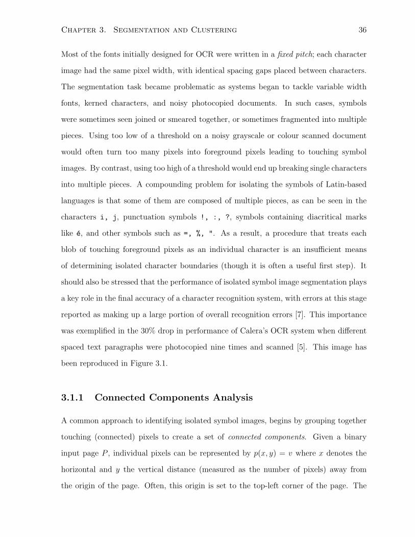
3.1 The impact of character spacing on recognition performance. Taken from
[5] . . . . . . . . . . . . . . . . . . . . . . . . . . . . . . . . . . . . . . . 37
ix
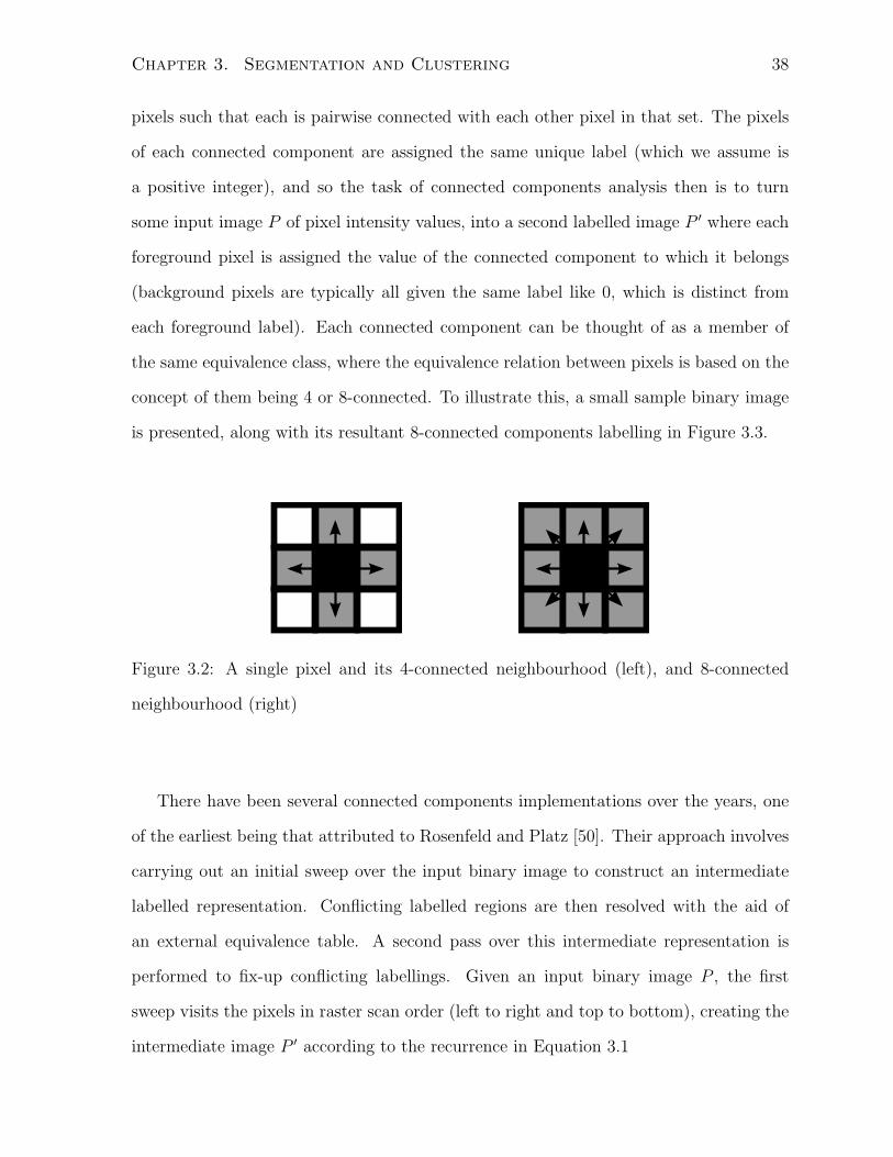
3.2 A single pixel and its 4-connected neighbourhood (left), and 8-connected
neighbourhood (right) . . . . . . . . . . . . . . . . . . . . . . . . . . . . 38
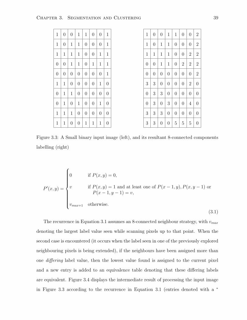
3.3 A Small binary input image (left), and its resultant 8-connected compo-
nents labelling (right) . . . . . . . . . . . . . . . . . . . . . . . . . . . . . 39
3.4 Resultant intermediate representation and equivalence table after perform-
ing a first sweep of the classical connected components algorithm [50] over
the input image in Figure 3.3 . . . . . . . . . . . . . . . . . . . . . . . . 41
3.5 Fused connected component, with horizontal and vertical projection pro-
files shown, as well as potential segmentation points found by minimal
projection profile . . . . . . . . . . . . . . . . . . . . . . . . . . . . . . . 45
3.6 Manhattan distance calculation between two grayscale images . . . . . . 51
3.7 Euclidean distance calculation between two grayscale images . . . . . . . 52
3.8 Hausdorff distance calculation between two binary images . . . . . . . . . 54
3.9 Hamming distances found under various padding schemes . . . . . . . . . 55
3.10 Histogram of horizontal space pixel widths found in a 15 page legal docu-
ment with a resolution of 196dpi . . . . . . . . . . . . . . . . . . . . . . . 57
3.11 Initial connected component regions identified for an input document image 59
3.12 Lines, baselines, and x-heights detected within part of a region identified
in Figure 2.8 . . . . . . . . . . . . . . . . . . . . . . . . . . . . . . . . . . 62
3.13 Updated connected components found for a small region after a vertical
merging procedure has occurred . . . . . . . . . . . . . . . . . . . . . . . 63
3.14 Cluster centroids and component counts found after performing a single
Euclidean and Hausdorff distance sweep over the components found in
Figure 3.13 . . . . . . . . . . . . . . . . . . . . . . . . . . . . . . . . . . 67
3.15 Cluster centroids and component counts found after iteratively performing
matches, merges and splits over the initial set of clusters and components
found in Figure 3.14 . . . . . . . . . . . . . . . . . . . . . . . . . . . . . 69
x
3.16 Randomly sampled set of cluster elements from each of the first 20 most
frequent clusters found when processing Figure 2.6 . . . . . . . . . . . . . 70
4.1 Upward concavities found in small samples of Roman (left) and Han-based
scripts (right) . . . . . . . . . . . . . . . . . . . . . . . . . . . . . . . . . 75
4.2 Sequence of component images and their corresponding cluster identifiers 77
5.1 Vote recognition accuracy as a function of document length . . . . . . . . 107
5.2 Histogram counts of number of clusters found per document . . . . . . . 108
5.3 Average vote based recognition accuracy calculated per cluster identifier . 108
5.4 Positional count recognition accuracy as a function of document length . 116
5.5 Average positional count based recognition accuracy calculated per cluster
identifier . . . . . . . . . . . . . . . . . . . . . . . . . . . . . . . . . . . . 117
5.6 Cross-word constraint recognition accuracy as a function of document length121
5.7 Average cross-word constraint recognition accuracy calculated per cluster
identifier . . . . . . . . . . . . . . . . . . . . . . . . . . . . . . . . . . . . 122
5.8 Recognition accuracy comparison between top-down and shape-based strate-
gies on UNLV dataset documents . . . . . . . . . . . . . . . . . . . . . . 125
5.9 Synthetic document cluster averages . . . . . . . . . . . . . . . . . . . . 126
5.10 Recognition accuracy comparison between top-down and shape-based strate-
gies on Reuters document images . . . . . . . . . . . . . . . . . . . . . . 128
xi
Chapter 1
Introduction
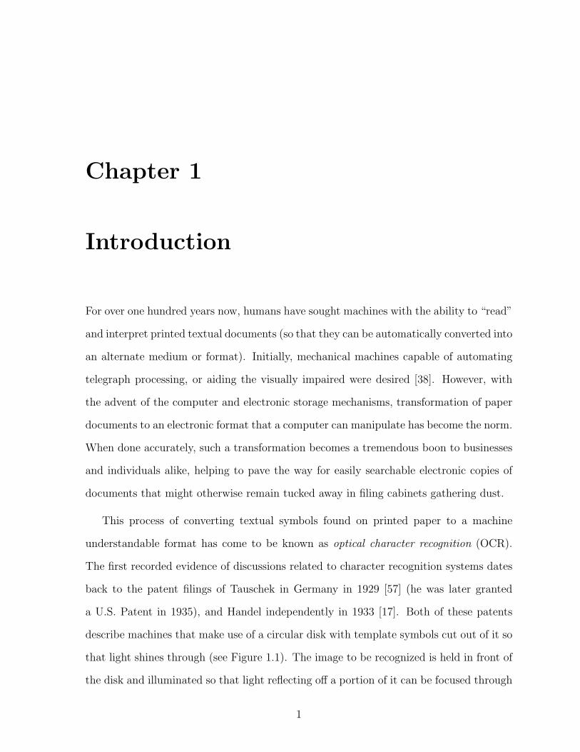
For over one hundred years now, humans have sought machines with the ability to “read”
and interpret printed textual documents (so that they can be automatically converted into
an alternate medium or format). Initially, mechanical machines capable of automating
telegraph processing, or aiding the visually impaired were desired [38]. However, with
the advent of the computer and electronic storage mechanisms, transformation of paper
documents to an electronic format that a computer can manipulate has become the norm.
When done accurately, such a transformation becomes a tremendous boon to businesses
and individuals alike, helping to pave the way for easily searchable electronic copies of
documents that might otherwise remain tucked away in filing cabinets gathering dust.
This process of converting textual symbols found on printed paper to a machine
understandable format has come to be known as optical character recognition (OCR).
The first recorded evidence of discussions related to character recognition systems dates
back to the patent filings of Tauschek in Germany in 1929 [57] (he was later granted
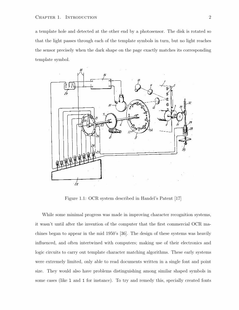
a U.S. Patent in 1935), and Handel independently in 1933 [17]. Both of these patents
describe machines that make use of a circular disk with template symbols cut out of it so
that light shines through (see Figure 1.1). The image to be recognized is held in front of
the disk and illuminated so that light reflecting off a portion of it can be focused through
1
Chapter 1. Introduction 2
a template hole and detected at the other end by a photosensor. The disk is rotated so
that the light passes through each of the template symbols in turn, but no light reaches
the sensor precisely when the dark shape on the page exactly matches its corresponding
template symbol.
Figure 1.1: OCR system described in Handel’s Patent [17]
While some minimal progress was made in improving character recognition systems,
it wasn’t until after the invention of the computer that the first commercial OCR ma-
chines began to appear in the mid 1950’s [36]. The design of these systems was heavily
influenced, and often intertwined with computers; making use of their electronics and
logic circuits to carry out template character matching algorithms. These early systems
were extremely limited, only able to read documents written in a single font and point
size. They would also have problems distinguishing among similar shaped symbols in
some cases (like l and 1 for instance). To try and remedy this, specially created fonts
Chapter 1. Introduction 3
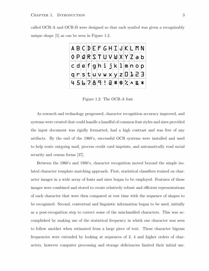
called OCR-A and OCR-B were designed so that each symbol was given a recognizably
unique shape [5] as can be seen in Figure 1.2.
Figure 1.2: The OCR-A font
As research and technology progressed, character recognition accuracy improved, and
systems were created that could handle a handful of common font styles and sizes provided
the input document was rigidly formatted, had a high contrast and was free of any
artifacts. By the end of the 1960’s, successful OCR systems were installed and used
to help route outgoing mail, process credit card imprints, and automatically read social
security and census forms [37].
Between the 1960’s and 1980’s, character recognition moved beyond the simple iso-
lated character template matching approach. First, statistical classifiers trained on char-
acter images in a wide array of fonts and sizes began to be employed. Features of these
images were combined and stored to create relatively robust and efficient representations
of each character that were then compared at test time with the sequence of shapes to
be recognized. Second, contextual and linguistic information began to be used, initially
as a post-recognition step to correct some of the misclassified characters. This was ac-
complished by making use of the statistical frequency in which one character was seen
to follow another when estimated from a large piece of text. These character bigram
frequencies were extended by looking at sequences of 3, 4 and higher orders of char-
acters, however computer processing and storage deficiencies limited their initial use.

Chapter 1. Introduction 4
Linguistic information in the form of simple word lookup was also employed to improve
OCR accuracy. Such an approach can be thought of as feeding the recognized sequence
of characters through a simple spell checker, with those words not found in the lookup
dictionary either flagged, or automatically corrected. Unfortunately this approach was
also limited due to computational constraints. By the mid 1980’s, these improvements
(among others) led to the introduction of so-called “omnifont” OCR systems capable of
recognizing characters from a vast array of font shapes and sizes [26], [5].
OCR systems and research have continued to improve over the years, and have now
reached a point that some researchers deem the recognition of machine printed character
images a largely solved problem [37]. Affordable commercial OCR software packages are
readily available, with some advertised claiming recognition accuracy rates above 99%.
While this state of affairs may lead one to believe that the use of character recognition
systems by businesses and individuals would be fairly widespread, the reality isn’t quite
so rosy. Recognition results are often quoted under “optimal” conditions, or are tested
against a sample of documents that do not necessarily match up to those seen in the real
world. In fact, given that documents can vary in terms of noise, layout, and complexity in
limitless ways it becomes near impossible to report a representative recognition accuracy.
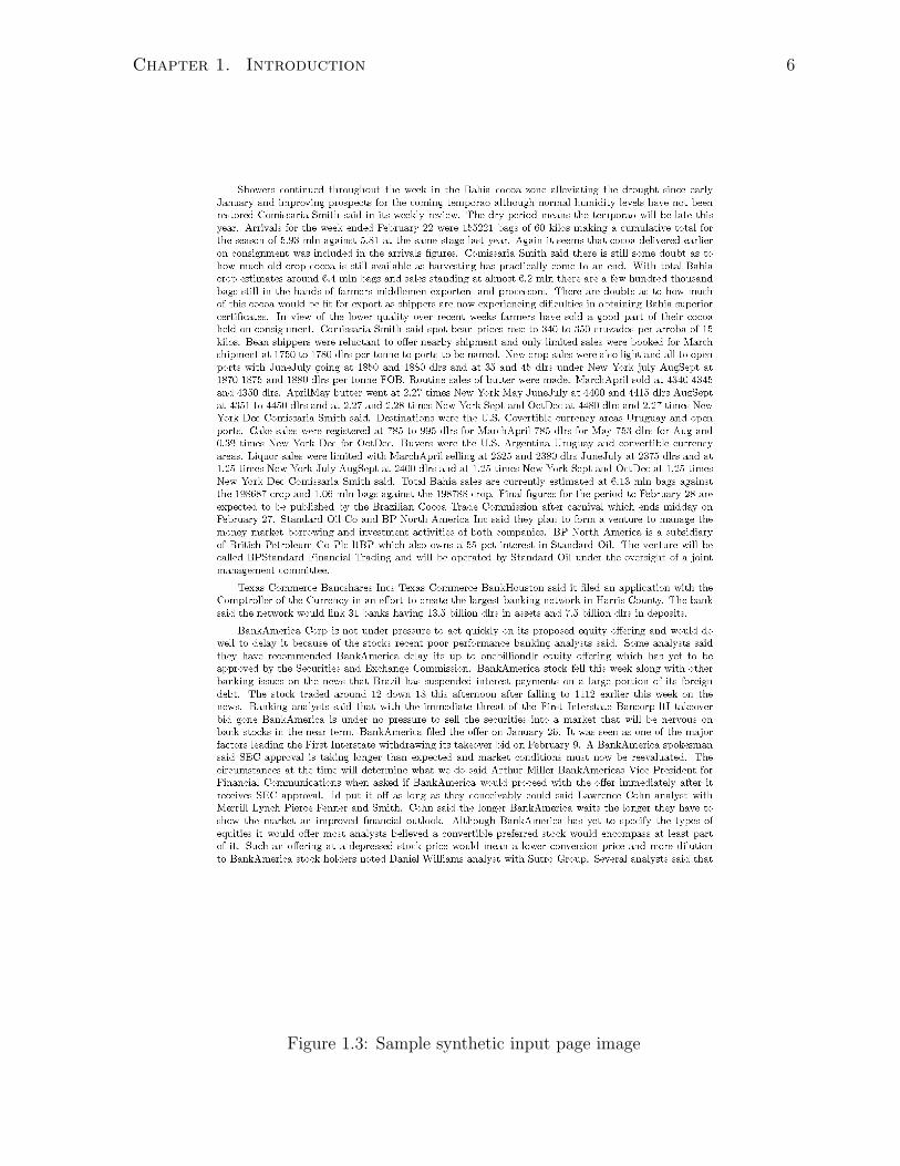
To further examine this, we conducted a simple experiment whereby a synthetic
document was constructed using text taken from the Reuters-21578 news corpus [34].
The document was typeset using Donald Knuth’s TEX typesetting system, and each page
was rendered as a single spaced, single column image written in the 10 point Computer
Modern typeface. Each page image was saved as a TIFF file with an output resolution
of 200 dots per inch (dpi). A sample page is presented in Figure 1.3. These page images
were then fed as input to several commercial and freely available OCR software packages.
The initial sequences of non-whitespace characters recognized by each package were then
compared with the first 19,635 non-whitespace characters belonging to the actual text
using tools from the OCRtk toolkit [42]. The resulting performance of each product
Chapter 1. Introduction 5
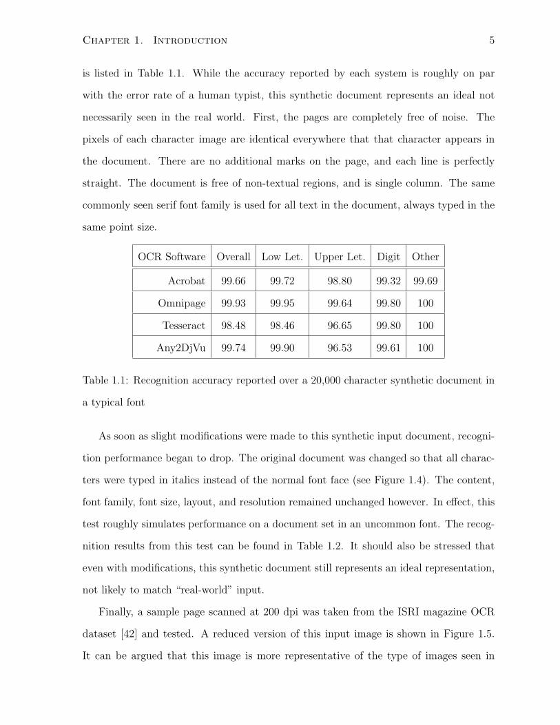
is listed in Table 1.1. While the accuracy reported by each system is roughly on par
with the error rate of a human typist, this synthetic document represents an ideal not
necessarily seen in the real world. First, the pages are completely free of noise. The
pixels of each character image are identical everywhere that that character appears in
the document. There are no additional marks on the page, and each line is perfectly
straight. The document is free of non-textual regions, and is single column. The same
commonly seen serif font family is used for all text in the document, always typed in the
same point size.
OCR Software Overall Low Let. Upper Let. Digit Other
Acrobat 99.66 99.72 98.80 99.32 99.69
Omnipage 99.93 99.95 99.64 99.80 100
Tesseract 98.48 98.46 96.65 99.80 100
Any2DjVu 99.74 99.90 96.53 99.61 100
Table 1.1: Recognition accuracy reported over a 20,000 character synthetic document in
a typical font
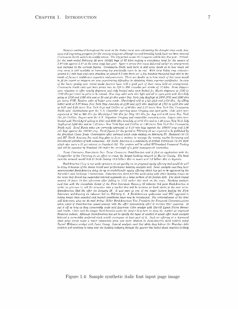
As soon as slight modifications were made to this synthetic input document, recogni-
tion performance began to drop. The original document was changed so that all charac-
ters were typed in italics instead of the normal font face (see Figure 1.4). The content,
font family, font size, layout, and resolution remained unchanged however. In effect, this
test roughly simulates performance on a document set in an uncommon font. The recog-
nition results from this test can be found in Table 1.2. It should also be stressed that
even with modifications, this synthetic document still represents an ideal representation,
not likely to match “real-world” input.
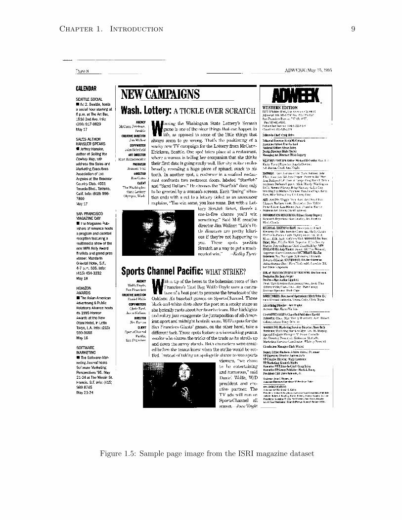
Finally, a sample page scanned at 200 dpi was taken from the ISRI magazine OCR
dataset [42] and tested. A reduced version of this input image is shown in Figure 1.5.
It can be argued that this image is more representative of the type of images seen in
Chapter 1. Introduction 6
Figure 1.3: Sample synthetic input page image
Chapter 1. Introduction 7
Figure 1.4: Sample synthetic italic font input page image
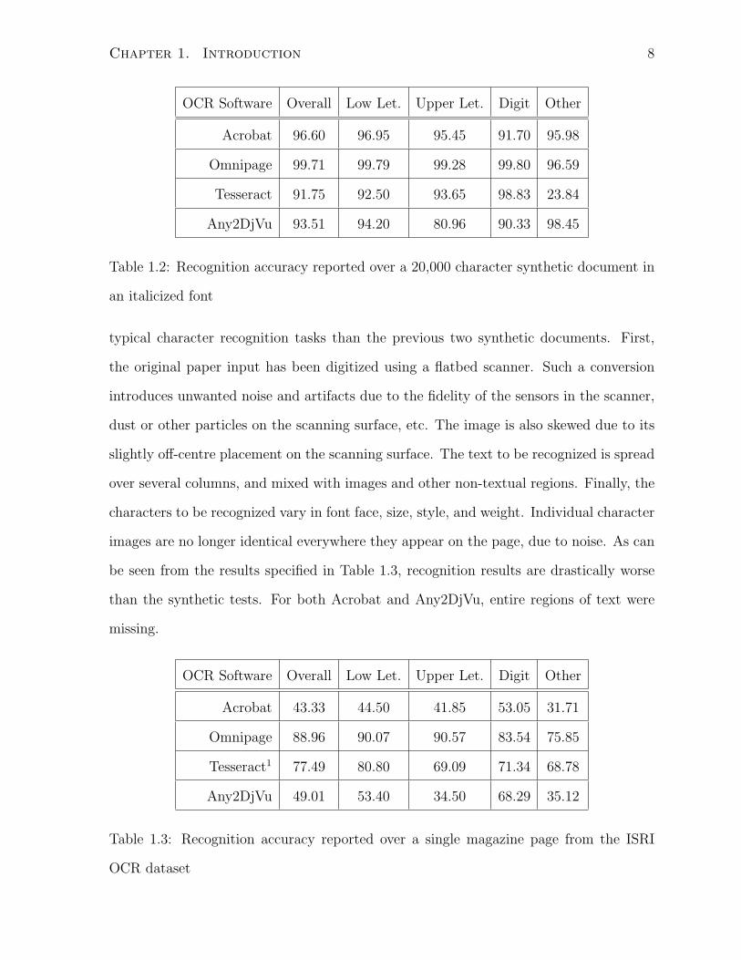
Chapter 1. Introduction 8
OCR Software Overall Low Let. Upper Let. Digit Other
Acrobat 96.60 96.95 95.45 91.70 95.98
Omnipage 99.71 99.79 99.28 99.80 96.59
Tesseract 91.75 92.50 93.65 98.83 23.84
Any2DjVu 93.51 94.20 80.96 90.33 98.45
Table 1.2: Recognition accuracy reported over a 20,000 character synthetic document in
an italicized font
typical character recognition tasks than the previous two synthetic documents. First,
the original paper input has been digitized using a flatbed scanner. Such a conversion
introduces unwanted noise and artifacts due to the fidelity of the sensors in the scanner,
dust or other particles on the scanning surface, etc. The image is also skewed due to its
slightly off-centre placement on the scanning surface. The text to be recognized is spread
over several columns, and mixed with images and other non-textual regions. Finally, the
characters to be recognized vary in font face, size, style, and weight. Individual character
images are no longer identical everywhere they appear on the page, due to noise. As can
be seen from the results specified in Table 1.3, recognition results are drastically worse
than the synthetic tests. For both Acrobat and Any2DjVu, entire regions of text were
missing.
OCR Software Overall Low Let. Upper Let. Digit Other
Acrobat 43.33 44.50 41.85 53.05 31.71
Omnipage 88.96 90.07 90.57 83.54 75.85
Tesseract1 77.49 80.80 69.09 71.34 68.78
Any2DjVu 49.01 53.40 34.50 68.29 35.12
Table 1.3: Recognition accuracy reported over a single magazine page from the ISRI
OCR dataset
Chapter 1. Introduction 9
Figure 1.5: Sample page image from the ISRI magazine dataset
Chapter 1. Introduction 10
While one cannot accurately judge performance on a few short pages of input, the
tremendous range in recognition accuracy reported by all systems should help illustrate
that the character recognition problem is still a ways off from truly being a solved one.
Steps must be taken to create robust recognition systems, able to perform accurately
across an incredibly vast range of possible inputs.
This thesis presents an exploration into improving the robustness of optical charac-
ter recognition. We do so by departing from the traditional bottom-up or shape-based
matching approach that has been present throughout the fifty plus year history of re-
search into recognition systems. Instead we focus fundamentally on exploiting contextual
cues and linguistic properties to determine the mapping from blobs of ink to underlying
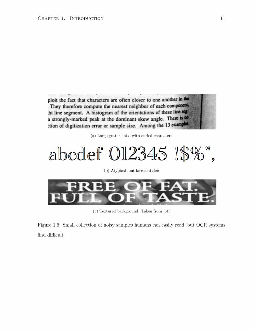
character symbols. This is largely motivated by human behaviour. We can effortlessly
read passages like those seen in Figure 1.6, or a sentence like f yu cn rd ths, yu’r smrtr
thn mst cr systms precisely because we appeal to context or language constraints. For a
language like English, we are readily aware that certain sequences of characters are much
more likely than others. We know that just about every word will contain at least one
vowel character, even that the ordering of words must follow a grammatical structure.
Instead of relying on shape information to do the heavy lifting during the recognition
process (with context being used as an afterthought to fill in the gaps and improve low
confidence mappings), we turn this approach on its head. Working in a top-down fashion
in which we completely ignore shape information during the recognition process, we in-
stead rely on contextual clues to do much of the work in determining character identities.
It is hoped that by operating in this manner, the recognition process will automatically
adapt to the specific nuances and constraints of each input document. Such a system be-
comes entirely independent of character font and shape, and with this variation removed,
improved robustness should result.
1Since Tesseract is currently limited to recognition of single column text, the input image was firstcropped into 3 separate column images
Chapter 1. Introduction 11
(a) Large gutter noise with curled characters
(b) Atypical font face and size
(c) Textured background. Taken from [61]
Figure 1.6: Small collection of noisy samples humans can easily read, but OCR systems
find difficult

Chapter 1. Introduction 12
1.1 Overview
The remainder of this thesis is structured as follows: In Chapter 2 we describe some of
the initial actions required to convert a paper document into a useful electronic version,
ready to have its characters recognized. This involves digitizing input pages, removing
noise and other artifacts, finding regions of text, then deskewing the regions so that lines
and characters are straight. In Chapter 3 we discuss techniques for isolating individual
character images, as well as grouping or clustering them together. This paves the way
for their subsequent recognition, which we describe in Chapter 4. We introduce three
new top-down recognition strategies each of which relies strongly on contextual and
other statistical language cues to determine the symbol that each cluster best represents.
Finally, in Chapter 5 we test the feasibility of our introduced approaches against several
real world and synthetic datasets containing documents from a variety of domains, fonts,
and quality levels. We tie all this work together in Chapter 6, where the advantages and
limitations of our proposed strategies, as well as areas for future work are discussed.
Chapter 2
Initial Document Processing
Before an OCR system can begin to recognize the symbols present in an input document
image, several important processing stages must be carried out to convert the input into
a usable form. While these processing stages do not represent the main focus of this
thesis, they are introduced and discussed in order to form a more complete picture of the
character recognition process.
2.1 Digitizing the Input
If the document to be recognized exists as a physical paper printout, the very first step
that must be carried out involves converting it to a representation that the recognition
system can manipulate. Since the majority of modern recognition systems are imple-
mented on computer hardware and software, this conversion of each page is typically to
some compressed or uncompressed digital image format. An uncompressed digital image
is stored on disk as a sequence of picture elements (pixels) each of which represents some
colour value. It should be noted that digital images are only approximations of their
original counterparts, albeit fairly accurate ones. The reason for this is the finite preci-
sion to which computers can store values. The continuous spectrum of colours that can
appear in nature, are quantized when stored digitally. Similarly, each pixel represents
13
Chapter 2. Initial Document Processing 14
some small but finite region of a page, and so any variability in smaller subregions will
remain unaccounted for. While these limitations rarely have an impact on the ability of
an OCR system to recognize the original symbols, trade-offs must be made between the
quality or fidelity of the digital image, and how efficiently it can be stored and processed
by a computer.
This conversion from printed page to digital image often involves specialized hardware
like an optical scanner that attempts to determine the colour value at evenly spaced points
on the page. The scanning resolution will determine how many of these points will be
inspected per unit of page length. Typically this is specified in dots or pixels per inch,
thus a document scanned at a resolution of 300dpi will have been sampled at 300 evenly
spaced points for each inch of each page. A standard US Letter sized (8.5 x 11 inch)
page scanned at 300dpi will have been sampled 8,415,000 times. At each of these sample
points or pixels the colour depth will determine to what extent the recognized colour
matches the true colour on the page. One of the more common colour depths involves
using a single byte to store each of the red, green and blue channels (plus an optional
additional byte used to store opacity information). Since each byte of storage is made
up of 8 bits, 28 = 256 unique shades of a colour can be represented. Since any colour can
be created by mixing red, green, and blue, the desired colour is approximated using the
closest shade of red, green, and blue. Note that colour depth is often measured in bits
per pixel (bpp), so our example above describes a 24bpp colour depth (32bpp if opacity
information is included).
While the optical scanner is the traditional means by which paper images become dig-
itized, there is an increasing trend in the use of digital cameras (including those attached
to cellular telephones) to capture and digitize document images [11]. These methods have
the advantage of being able to capture documents (like thick books, product packaging
or road signs) that might prove difficult or impossible using a flatbed scanner. Brewster
Chapter 2. Initial Document Processing 15
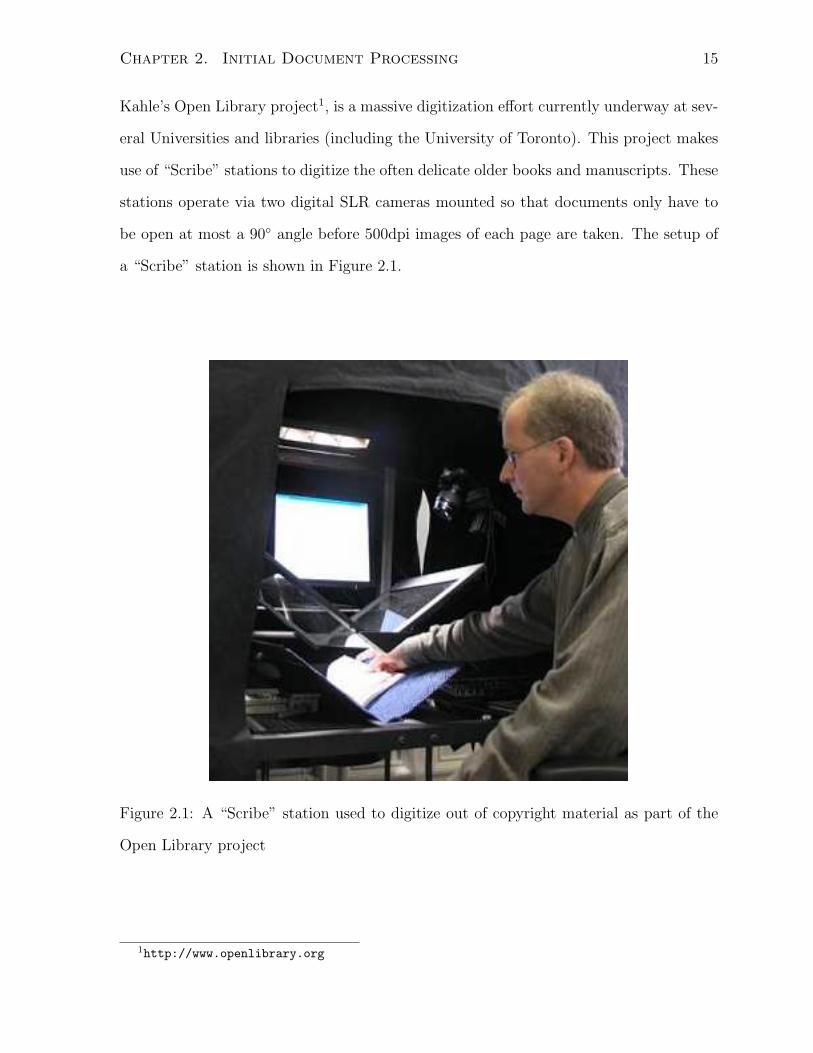
Kahle’s Open Library project1, is a massive digitization effort currently underway at sev-
eral Universities and libraries (including the University of Toronto). This project makes
use of “Scribe” stations to digitize the often delicate older books and manuscripts. These
stations operate via two digital SLR cameras mounted so that documents only have to
be open at most a 90 angle before 500dpi images of each page are taken. The setup of
a “Scribe” station is shown in Figure 2.1.
Figure 2.1: A “Scribe” station used to digitize out of copyright material as part of the
Open Library project
1http://www.openlibrary.org
Chapter 2. Initial Document Processing 16
2.1.1 Binarization
For character recognition purposes, one generally does not need a full colour represen-
tation of the image, and so pages are often scanned or converted to a grayscale (8bpp),
or bilevel (1bpp) colour depth. In grayscale, each pixel represents one of 256 shades of
gray, and in a bilevel image each pixel is assigned one of two values representing black or
white. While both of these methods will allow a digital image to be stored in a smaller
space (fewer bpp), they can suffer from information loss as the original colour value is
more coarsely approximated. Working with bilevel images is particularly efficient, and
some processing algorithms are restricted to this format.
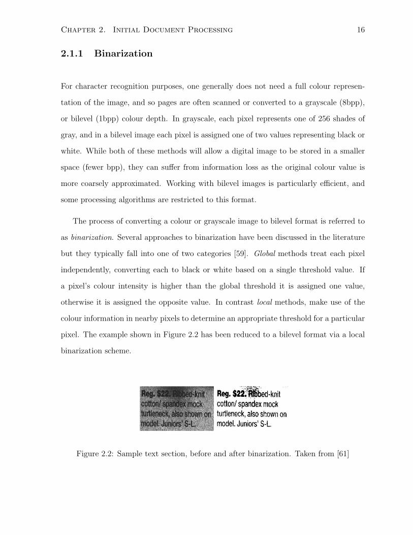
The process of converting a colour or grayscale image to bilevel format is referred to
as binarization. Several approaches to binarization have been discussed in the literature
but they typically fall into one of two categories [59]. Global methods treat each pixel
independently, converting each to black or white based on a single threshold value. If
a pixel’s colour intensity is higher than the global threshold it is assigned one value,
otherwise it is assigned the opposite value. In contrast local methods, make use of the
colour information in nearby pixels to determine an appropriate threshold for a particular
pixel. The example shown in Figure 2.2 has been reduced to a bilevel format via a local
binarization scheme.
Figure 2.2: Sample text section, before and after binarization. Taken from [61]
Chapter 2. Initial Document Processing 17
2.1.2 Textured Backgrounds
A related problem facing character recognition systems is the separation of text from a
textured or decorated background. See Figure 1.6c for an example. Not only can tex-
tured backgrounds prohibit accurate binarization of input document images (particularly
skewing global threshold based approaches), but they make segmentation and recognition
of characters much more difficult.
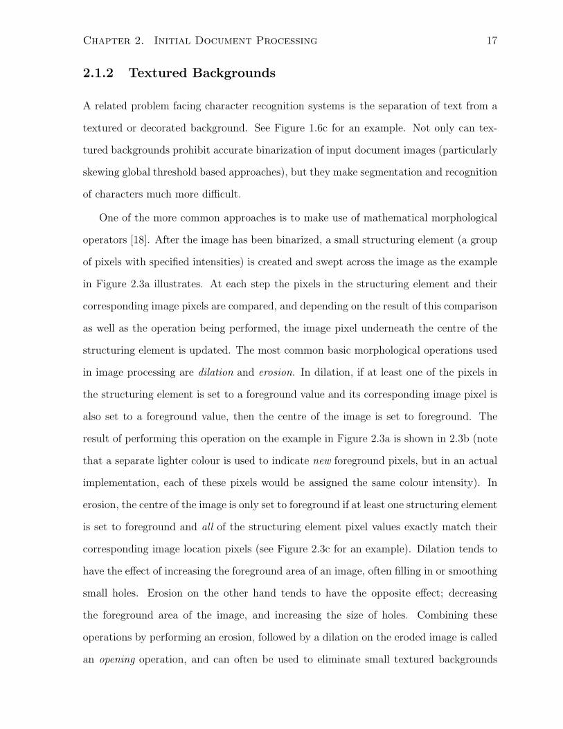
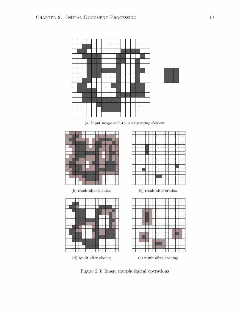
One of the more common approaches is to make use of mathematical morphological
operators [18]. After the image has been binarized, a small structuring element (a group
of pixels with specified intensities) is created and swept across the image as the example
in Figure 2.3a illustrates. At each step the pixels in the structuring element and their
corresponding image pixels are compared, and depending on the result of this comparison
as well as the operation being performed, the image pixel underneath the centre of the
structuring element is updated. The most common basic morphological operations used
in image processing are dilation and erosion. In dilation, if at least one of the pixels in
the structuring element is set to a foreground value and its corresponding image pixel is
also set to a foreground value, then the centre of the image is set to foreground. The
result of performing this operation on the example in Figure 2.3a is shown in 2.3b (note
that a separate lighter colour is used to indicate new foreground pixels, but in an actual
implementation, each of these pixels would be assigned the same colour intensity). In
erosion, the centre of the image is only set to foreground if at least one structuring element
is set to foreground and all of the structuring element pixel values exactly match their
corresponding image location pixels (see Figure 2.3c for an example). Dilation tends to
have the effect of increasing the foreground area of an image, often filling in or smoothing
small holes. Erosion on the other hand tends to have the opposite effect; decreasing
the foreground area of the image, and increasing the size of holes. Combining these
operations by performing an erosion, followed by a dilation on the eroded image is called
an opening operation, and can often be used to eliminate small textured backgrounds
Chapter 2. Initial Document Processing 18
from foreground text to reasonably good effect. A synthetic example of the opening
operation is shown in Figure 2.3e.
In recent work by Wu and Manmatha [61], an alternate approach to separating text
from textured backgrounds and binarizing an input image was described. First a smooth-
ing low-pass Gaussian filter was passed over the image. Then the resultant histogram of
image intensities was smoothed (again using a low-pass filter). The valley after the first
peak in this smoothed histogram was then sought, and used to differentiate foreground
text from background.
2.2 Noise Removal
During the scanning process, differences between the digital image and the original input
(beyond those due to quantization when stored on computer) can occur. Hardware or
software defects, dust particles on the scanning surface, improper scanner use, etc. can
change pixel values from those that were expected. Such unwanted marks and differing
pixel values constitute noise that can potentially skew character recognition accuracy.
Furthermore, certain marks or anomalies present in the original document before being
scanned (from staples, or telephone line noise during fax transmission etc.) constitute
unwanted blemishes or missing information that one may also like to rectify and correct
before attempting character recognition.
There are typically two approaches taken to remove unwanted noise from document
images. For pixels that have been assigned a foreground value when a background value
should have been given (additive noise), correction can sometimes be accomplished by
removing any groups of foreground pixels that are smaller than some threshold. These
groups of foreground pixels can be identified by employing a connected component sweep
over the document (see Chapter 3). Care must be taken to ensure that groups of pixels
corresponding to small parts of characters or symbols (dots above i, or j, or small
Chapter 2. Initial Document Processing 19
(a) Input image and 3× 3 structuring element
(b) result after dilation (c) result after erosion
(d) result after closing (e) result after opening
Figure 2.3: Image morphological operations
Chapter 2. Initial Document Processing 20
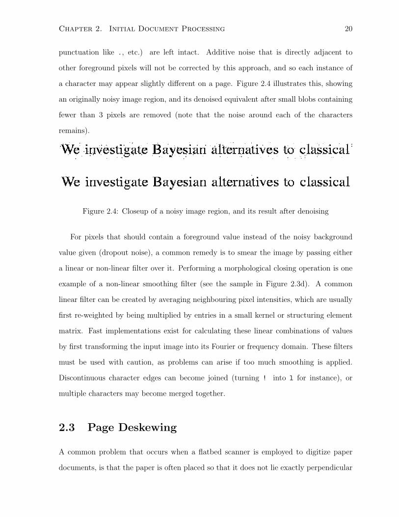
punctuation like ., etc.) are left intact. Additive noise that is directly adjacent to
other foreground pixels will not be corrected by this approach, and so each instance of
a character may appear slightly different on a page. Figure 2.4 illustrates this, showing
an originally noisy image region, and its denoised equivalent after small blobs containing
fewer than 3 pixels are removed (note that the noise around each of the characters
remains).
Figure 2.4: Closeup of a noisy image region, and its result after denoising
For pixels that should contain a foreground value instead of the noisy background
value given (dropout noise), a common remedy is to smear the image by passing either
a linear or non-linear filter over it. Performing a morphological closing operation is one
example of a non-linear smoothing filter (see the sample in Figure 2.3d). A common
linear filter can be created by averaging neighbouring pixel intensities, which are usually
first re-weighted by being multiplied by entries in a small kernel or structuring element
matrix. Fast implementations exist for calculating these linear combinations of values
by first transforming the input image into its Fourier or frequency domain. These filters
must be used with caution, as problems can arise if too much smoothing is applied.
Discontinuous character edges can become joined (turning ! into l for instance), or
multiple characters may become merged together.
2.3 Page Deskewing
A common problem that occurs when a flatbed scanner is employed to digitize paper
documents, is that the paper is often placed so that it does not lie exactly perpendicular
Chapter 2. Initial Document Processing 21
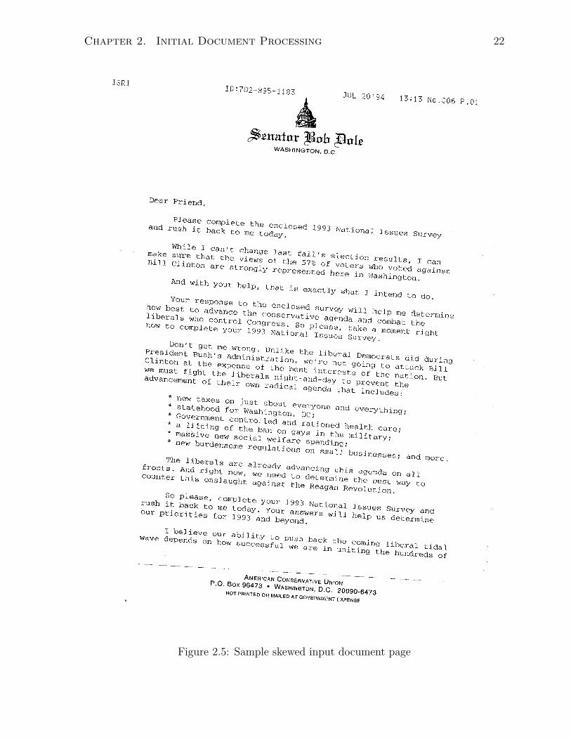
with the scanner head. Instead it is often rotated some arbitrary angle, so that when
scanned the resultant digitized document image appears skewed (see Figure 2.5). De-
pending on the algorithms employed, working with skewed documents directly can lead
to difficulties when attempts are made to segment the input image into columns, lines,
words or individual character regions. One simple illustration of this is the (naive) at-
tempt of creating a line finder that works by summing pixel intensity values horizontally
across each row of pixels, then scanning these sums vertically to find consecutive valleys
or runs of minimal sum (this assumes the document to be recognized has a horizontal
reading order). For unskewed documents consisting of single column text written in a
horizontal fashion, this approach should allow one to determine line boundaries by find-
ing the start of the minimal sum valleys. However, if the document has been scanned
so that its digital representation is skewed, then profile sums across each row of pixels
will no longer contain sharp minimal valleys. If the skew is large enough that each row
of pixels contains portions of two or more lines of text, then the profile sums will look
somewhat more uniform, and one will not be able to identify the line boundaries. Skewed
documents can also impact character recognition performance. If the approach attempts
to group similar shaped symbol images together so that each instance can be assigned a
single label, then multiple page documents that have been scanned so that each page has
a different skew angle will result in slightly altered (rotated) shape images for the same
symbol.
Many of the earliest attempts at identifying document skew angle exploited the regu-
larity with which the lines of text were oriented on a page. By using the Hough transform
[12], pixels aligned along an arbitrary skew angle could be found fairly efficiently. The
Hough transform works by transforming each pixel in image space, into a sinusoidal curve
in an equivalent parameter space. Specifically, each pixel xi, yi in the image gets mapped
to a sinusoidal curve r = xi cos θ + yi sin θ where the parameters define a straight line
lying a distance r from the origin, and oriented perpendicular to the angle θ. The nice
Chapter 2. Initial Document Processing 22
Figure 2.5: Sample skewed input document page
Chapter 2. Initial Document Processing 23
property resulting from this representation is that image points that lie along the same
straight line, will have their sinusoidal curves intersect at a common point in parameter
space. By looking in this space for places where many of the curves intersect, one can
then determine the dominant angle of skew of the page.
In 1987, Baird [2] described a method for skew estimation that first calculated the
connected components of each page image (see Chapter 3 for a discussion of how con-
nected components can be found). By selecting the bottom middle co-ordinate point of
the bounding box around each of these components, the number of these points found
to lie near lines of a particular angle can be found. As the angle is changed, the squared
sum of the number of points lying along that angle will change, but it will be maximal
near angles that constitute dominant text orientation lines. Instead of attempting to
sum pixels along some arbitrary angle, the image is first sheared vertically by the angle,
and a projection is taken horizontally to estimate the number of pixels lying along that
particular line. Finding this maximal sum value then amounts to finding the skew angle
for most document images.
An alternate approach that works independently of the amount of skew was intro-
duced by Hashizume [19]. Under the assumption that the distance between lines of text
is greater than the distance between characters on the same line, their approach sets
out first to determine the connected components on a page, then find the angle of the
straight-line drawn to connect the centres of the bounding boxes of the single nearest
neighbour of each component. A histogram of these angles is constructed, with the modal
value representing the dominant document skew angle. This fairly simple approach works
well provided the document is mostly text, though its performance can rapidly deterio-
rate when image regions are included, or many touching characters are present yielding
interline distances roughly on par with the perpendicular distance between these multi-
character components.
In 1995, Bloomberg et al [4] introduced and applied to 1,000 page images, a slightly
Chapter 2. Initial Document Processing 24
modified version of skew detection first presented by Postl in a patent application [46].
Postl and Bloomberg’s implementations are similar to Baird’s in that they all work to
find skew angle by locating lines in the image. However, instead of taking squared
sums across the rows of individual connected components as the angle changes, Postl
and Bloomberg take the difference between the row values when summing across all
foreground pixels along a particular line as the angle changes. Bloomberg increases the
efficiency over Postl’s original implementation by first subsampling and smoothing the
image. The dominant angle can then be found as the angle that leads to the largest
difference between subsequent row sums. This is easy to understand if one imagines
comparing the sum of pixels along an aligned row of text with the sum of pixels along a
row between lines of text. The former will have a large sum, while the latter will have
a minimal or zero sum. If the angle is skewed so that rows now cross text lines, this
will end up smoothing out the difference in such sums since both rows will likely cross
portions of the text that both cover characters, and the blank spaces between lines of
characters.
More recently, Amin and Wu [1] introduced an approach to skew detection that was
shown to be robust to document images that contain a mixture of text and graphics, even
documents with regions belonging to the same page that are skewed in different directions.
After identifying regions of the input image in a bottom-up fashion (see Section 2.4 for a
discussion of region detection), the regions are rotated, and a rectangular bounding box
is drawn tightly around the region to be deskewed. Their method exploits the property
that even though the area of the region itself remains constant during rotation, the area
of the bounding box is at a minimum when the object is aligned in one of the four
principal directions. By trying all possible rotations in a fixed degree of increment, the
minimum can be found. Drawbacks of their approach include not handling regions that
do not contain a primary direction (like circular regions), as well as the computational
cost required to try each possible rotation for each region of interest.
Chapter 2. Initial Document Processing 25
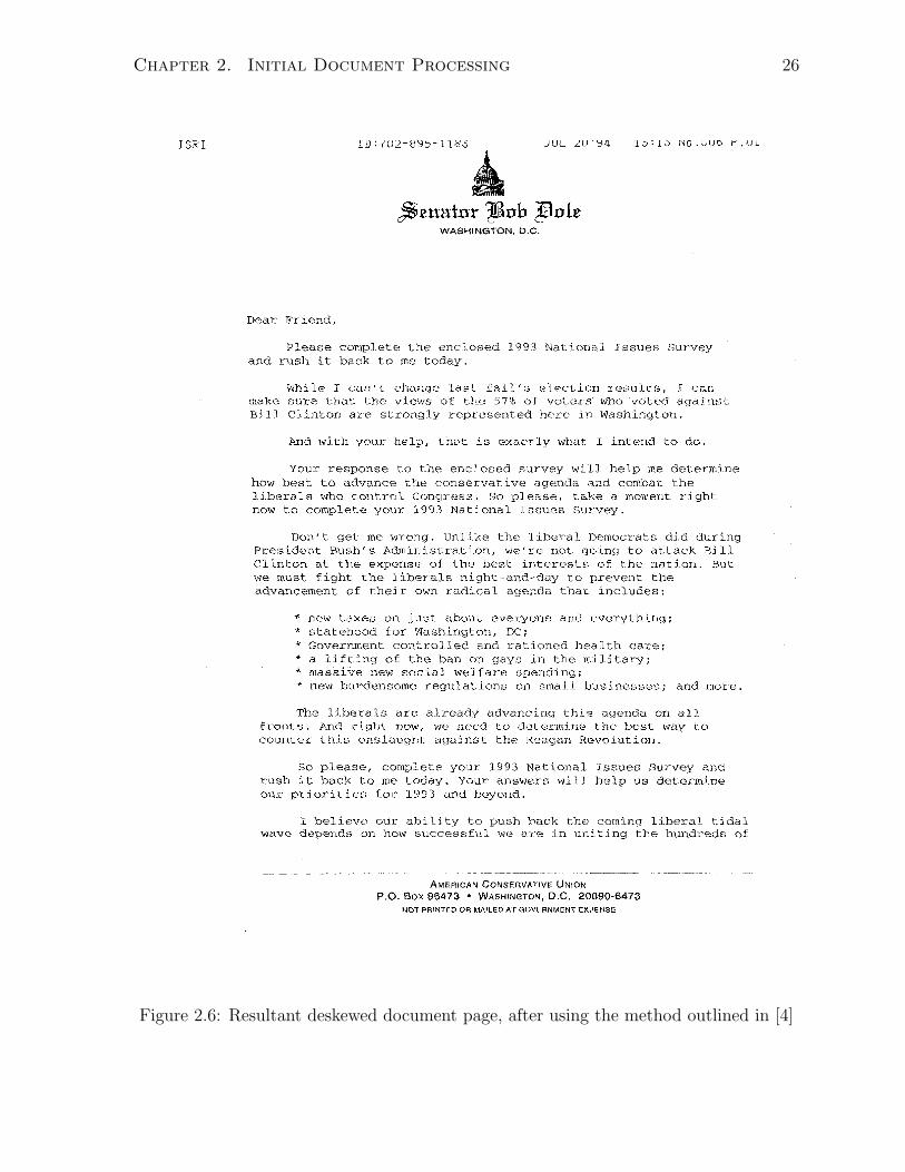
For the most part, many of the approaches discussed can accurately identify the
skew angle in documents that are mostly text written in a single direction, however
most methods of correcting this skew often involve nothing more than a single shear
transformation on the image pixels. While this will orient the lines of the text, the
individual character images may become inconsistent as seen in the sample in Figure 2.6
(take a close look at some of the e images for instance).
2.4 Geometric Layout Analysis
Once a page has been digitized, denoised, and deskewed, the final remaining preprocessing
task involves identifying the regions of text to be extracted from the page. Like most of
the other phases of document analysis, there are many ways to attempt to tackle this
problem, and doing so leads naturally into the follow-up tasks of isolating and segmenting
the lines, words, and individual character images for the purposes of recognizing them.
Textual region identification can become an intricate procedure due in part to the endless
variety of document images that can be presented. While large, single column paragraphs
of body copy may be fairly trivial to pick out of a document image, this process becomes
increasingly more complex as one tries to extract the contents of tables, figure captions,
text appearing within a graph or halftone image, etc. In multi-column documents and
documents containing figure captions, determining the correct reading order of the text
is non-trivial. Care must be taken to ensure that the recognized text does not insert a
figure caption between two body text paragraphs, or does not cross column boundaries
resulting in non-sensical text strings interleaved from disparate paragraphs. The entire
textual region and reading order identification process is often given the term zoning
[8]. In the discussion that follows, we use the term “region” to mean a maximally sized
grouping of neighbouring pixels such that each pixel in the group belongs to the same
class type, e.g. the group of pixels composing a paragraph of text, or a graph for instance.
Chapter 2. Initial Document Processing 26
Figure 2.6: Resultant deskewed document page, after using the method outlined in [4]
Chapter 2. Initial Document Processing 27
We assume that region boundaries are rectangular in nature unless otherwise stated.
Identifying textual regions first requires that the pixels on a page become partitioned
into disjoint groups (a process called page segmentation). Methods for performing this
grouping often fall under one of two opposing paradigms. In top-down approaches, all
the pixels are initially placed into the same group, which is repeatedly split apart until
each group contains pixels resembling a homogeneous region of the page. In contrast,
bottom-up methods initially place each pixel into a separate group, which are merged
together until a sensible region partitioning exists.
The run-length smoothing algorithm introduced by Wong et al [60] was one of the
first bottom-up approaches used to identify page regions. This simple algorithm makes
two passes over a binary input page, one smearing the foreground pixels vertically and
the other horizontally, resulting in two intermediate copies of the original image. The
smearing process leaves the original foreground pixels untouched, but for each background
pixel that is closer than some threshold number of pixels from an adjacent foreground
pixel, its value is changed to a foreground intensity (the remaining background pixels
retain their original intensity). These two intermediate images are overlaid, and a logical
AND operation is performed on the overlapping foreground pixels to produce a final
intensity image upon which a second horizontal smearing and connected components
analysis is run to determine final region boundaries.
One of the earliest top-down approaches introduced by Nagy and Seth in 1984 [39],
attempted to carve a document into regions by recursively performing either a horizontal
or vertical cut inside of the regions defined by previous cuts (with the cut performed
in the direction opposite the previous cut). This led to a data structure representation
called an XY-tree, whose nodes represent rectangular page subregions (the root being
the region defined by the entire page). The children of a given node are determined by
summing the foreground pixels across that region in a single direction, then scanning
down that sum for large valleys or runs of consecutive minimal value. Runs longer
Chapter 2. Initial Document Processing 28
than a particular threshold are identified, and cuts are made at their centres so that
new child regions are created between successive cuts. This process then repeats by
summing across these child regions in the orthogonal direction and cutting until no
valleys larger than the threshold length remain. The leaves of this tree then represent
the final set of segmentation rectangles for the page image. Often, two different thresholds
are employed, one for the horizontal cuts and one for vertical reflecting the difference in
gap sizes between foreground pixels in each direction. This work was later extended by
Cesarani et al [9] to process subregions inside enclosed structures like tables. One of the
biggest drawbacks to the traditional XY-tree approach is its failure to segment a page
that contains long black strips around the margins when scanned (see the discussion in
Section 2.2 for further details). Such noisy regions prevent the appearance of valleys
when sums are taken perpendicular to them and this may halt the cutting process for
that region [52].
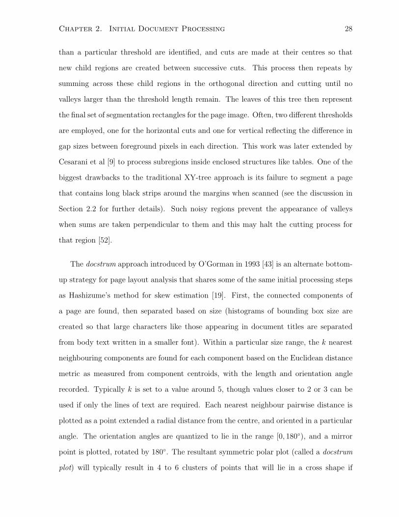
The docstrum approach introduced by O’Gorman in 1993 [43] is an alternate bottom-
up strategy for page layout analysis that shares some of the same initial processing steps
as Hashizume’s method for skew estimation [19]. First, the connected components of
a page are found, then separated based on size (histograms of bounding box size are
created so that large characters like those appearing in document titles are separated
from body text written in a smaller font). Within a particular size range, the k nearest
neighbouring components are found for each component based on the Euclidean distance
metric as measured from component centroids, with the length and orientation angle
recorded. Typically k is set to a value around 5, though values closer to 2 or 3 can be
used if only the lines of text are required. Each nearest neighbour pairwise distance is
plotted as a point extended a radial distance from the centre, and oriented in a particular
angle. The orientation angles are quantized to lie in the range [0, 180), and a mirror
point is plotted, rotated by 180. The resultant symmetric polar plot (called a docstrum
plot) will typically result in 4 to 6 clusters of points that will lie in a cross shape if
Chapter 2. Initial Document Processing 29
the document has a 0 skew angle. The relative orientation of these clusters can be
used to determine overall page skew, as well as estimate inter-character, inter-word, and
inter-line space width. After page skew is estimated, text lines are found by forming
the transitive closure on neighbouring components lying roughly along the skew angle.
The centroids of each resultant group component are joined by least squares fit straight
lines. These text lines are then merged by finding other text lines that fall within a small
perpendicular distance threshold, and lie roughly parallel (as measured by a parallel
distance threshold). Unlike some of the previously discussed approaches, the docstrum
method does not require an explicit hand-set threshold for determining inter-character
and inter-line space width estimation, instead this is found automatically as part of the
process. Another nice feature of this approach is that skew estimation is found as part of
the process. It can easily be extended via a preprocessing stage to run within subregions
of a page, allowing one to handle separate sections of a page that contain different skew
angles. A major drawback of the docstrum approach is that it requires prior identification
and removal of images and other graphics from the page before processing (which really
defeats the purpose of using it to separate textual from non-textual regions).
A reliable page segmentation strategy that is not limited to rectangular shaped re-
gions is the area Voronoi diagram approach introduced by Kise et al [27]. Connected
components are found, then the outer boundary along each of these components is sam-
pled at a regular interval. A set of edges is circumscribed around each sampled point
creating a Voronoi region V (p), defined as in Equation 2.1.
V (p) = x|d(x, p) ≤ d(x, q), ∀q 6= p (2.1)
In Equation 2.1 p, q are sample boundary points, x is a point on the page, and d(a, b) is
defined to be the Euclidean distance between points a and b. Thus, the boundary Voronoi
edges lie exactly midway between the sampled point and its closest neighbouring sample
point. The edges created between sample points belonging to the same component are
Chapter 2. Initial Document Processing 30
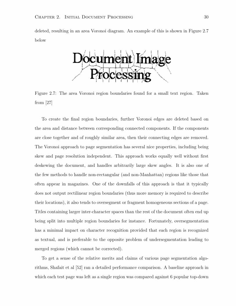
deleted, resulting in an area Voronoi diagram. An example of this is shown in Figure 2.7
below
Figure 2.7: The area Voronoi region boundaries found for a small text region. Taken
from [27]
To create the final region boundaries, further Voronoi edges are deleted based on
the area and distance between corresponding connected components. If the components
are close together and of roughly similar area, then their connecting edges are removed.
The Voronoi approach to page segmentation has several nice properties, including being
skew and page resolution independent. This approach works equally well without first
deskewing the document, and handles arbitrarily large skew angles. It is also one of
the few methods to handle non-rectangular (and non-Manhattan) regions like those that
often appear in magazines. One of the downfalls of this approach is that it typically
does not output rectilinear region boundaries (thus more memory is required to describe
their locations), it also tends to oversegment or fragment homogeneous sections of a page.
Titles containing larger inter-character spaces than the rest of the document often end up
being split into multiple region boundaries for instance. Fortunately, oversegmentation
has a minimal impact on character recognition provided that each region is recognized
as textual, and is preferable to the opposite problem of undersegmentation leading to
merged regions (which cannot be corrected).
To get a sense of the relative merits and claims of various page segmentation algo-
rithms, Shafait et al [52] ran a detailed performance comparison. A baseline approach in
which each test page was left as a single region was compared against 6 popular top-down
Chapter 2. Initial Document Processing 31
and bottom-up approaches including XY-tree cutting, run-length smoothing, whitespace
analysis, constrained text-line finding, docstrum, and area Voronoi diagram based ap-
proaches. The authors calculated errors based on text line and ignored non-textual region
detection completely. For each contiguous line of text, an error was counted if it either
did not belong to any region (missed), was split into two or more region bounding boxes
(split), or was found contained within a region bounding box that also contained another
horizontally adjacent text line (merged). Note that multiple text lines merged vertically
within a single region boundary were not counted as errors, thus for single column pages,
the dummy algorithm would achieve a low error score. The error score was defined to be
the percentage of text-lines that were either missed, split, or merged. Each algorithm was
tested against 978 page images from the University of Washington UW-III database [45].
The set was split into 100 training and 878 testing images, with the training set used
to find optimal parameter settings for each method. While no single method was shown
to be significantly better than the others (due to large performance variation across in-
dividual pages), both the docstrum and Voronoi approaches had average optimized test
performance scores lower than 6%. All approaches performed better than the dummy
implementation, but both XY-cuts and smearing tended to perform the worst (average
test scores of 17.1 and 14.2% respectively).
Once a suitable region partitioning of a page has been found, each region must then
be labelled as belonging to a particular region type (a process often termed page or region
classification). For basic character recognition purposes, distinguishing between textual
and non-textual region types is the minimal requirement. A naive and inefficient way of
determining this involves simply running a character recognition process on each region,
and if a significant portion of confident mappings can not be found, the region should be
discarded as being non-textual. Less involved methods of determining whether a region is
textual exploit the periodic structure of pixels inside these regions. For example regions
written in Latin-based alphabets will consist of approximately evenly spaced horizontal
Chapter 2. Initial Document Processing 32
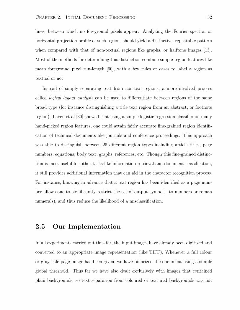
lines, between which no foreground pixels appear. Analyzing the Fourier spectra, or
horizontal projection profile of such regions should yield a distinctive, repeatable pattern
when compared with that of non-textual regions like graphs, or halftone images [13].
Most of the methods for determining this distinction combine simple region features like
mean foreground pixel run-length [60], with a few rules or cases to label a region as
textual or not.
Instead of simply separating text from non-text regions, a more involved process
called logical layout analysis can be used to differentiate between regions of the same
broad type (for instance distinguishing a title text region from an abstract, or footnote
region). Laven et al [30] showed that using a simple logistic regression classifier on many
hand-picked region features, one could attain fairly accurate fine-grained region identifi-
cation of technical documents like journals and conference proceedings. This approach
was able to distinguish between 25 different region types including article titles, page
numbers, equations, body text, graphs, references, etc. Though this fine-grained distinc-
tion is most useful for other tasks like information retrieval and document classification,
it still provides additional information that can aid in the character recognition process.
For instance, knowing in advance that a text region has been identified as a page num-
ber allows one to significantly restrict the set of output symbols (to numbers or roman
numerals), and thus reduce the likelihood of a misclassification.
2.5 Our Implementation
In all experiments carried out thus far, the input images have already been digitized and
converted to an appropriate image representation (like TIFF). Whenever a full colour
or grayscale page image has been given, we have binarized the document using a simple
global threshold. Thus far we have also dealt exclusively with images that contained
plain backgrounds, so text separation from coloured or textured backgrounds was not
Chapter 2. Initial Document Processing 33
investigated.
In our experiments, many of the pages given were generated from perfectly aligned
PDF originals, thus page deskewing was largely not implemented. When testing against
some of the ISRI OCR datasets [42], page images were first deskewed using the implemen-
tation in the Leptonica2 image processing libraries. This library uses the implementation
discussed by Bloomberg et al [4].
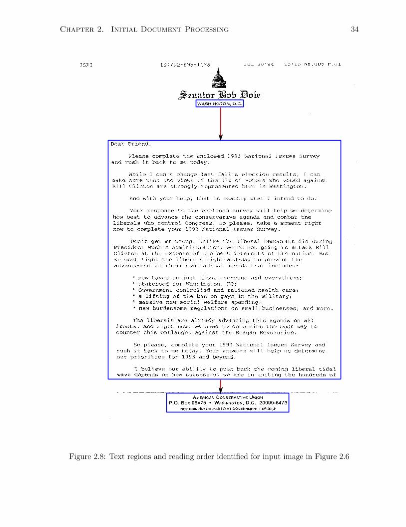
For the majority of our experiments, we were given ground-truth region information.
In such cases we made direct use of this instead of trying to detect textual zones upon
which to perform further processing. If these regions were available for a page, our
implementation would remove the foreground pixels from all areas on the page, except
those regions that were labelled as text. When testing documents for which no ground-
truth region and zoning information was available, for the most part we made use of the
JTAG [29] software package to automatically find a list of textual regions. The JTAG
software implementation performs page segmentation using recursive cuts applied to the
XY-tree (the horizontal and vertical cutting thresholds were set manually, depending on
the document being processed). After textual regions were identified, their reading order
was set manually by inspection. The results of running region detection on the input
image originally given in Figure 2.6 is shown in Figure 2.8.
2http://www.leptonica.org
Chapter 2. Initial Document Processing 34
Figure 2.8: Text regions and reading order identified for input image in Figure 2.6
Chapter 3
Segmentation and Clustering
Once a page has been suitably digitized, cleaned up, and had its textual regions located,
it is ready to be segmented so that the individual symbols of interest can be extracted and
subsequently recognized. In this chapter we focus on locating these isolated character
images and related features like word and line boundaries. We also describe our approach
to grouping these isolated images together so that there is only one (or a few) such rep-
resentatives for each character symbol. It is at this stage, that our character recognition
strategy begins to distinguish itself from classical or historically driven approaches to
recognition. Such systems typically do not make attempts to cluster similar shapes to-
gether, instead they move directly to the recognition of isolated character images (via
image shape features).
3.1 Isolated Symbol Image Segmentation
With non-textual and other noise regions removed, this section discusses how a document
image is further segmented so that each region corresponds to the bitmap of a single
character. In the early days of OCR, input documents were heavily constrained so that
individual characters could be isolated without too much difficulty. Many forms contained
rectangular bounding boxes, forcing the user to type or print a single character per box.
35
Chapter 3. Segmentation and Clustering 36
Most of the fonts initially designed for OCR were written in a fixed pitch; each character
image had the same pixel width, with identical spacing gaps placed between characters.
The segmentation task became problematic as systems began to tackle variable width
fonts, kerned characters, and noisy photocopied documents. In such cases, symbols
were sometimes seen joined or smeared together, or sometimes fragmented into multiple
pieces. Using too low of a threshold on a noisy grayscale or colour scanned document
would often turn too many pixels into foreground pixels leading to touching symbol
images. By contrast, using too high of a threshold would end up breaking single characters
into multiple pieces. A compounding problem for isolating the symbols of Latin-based
languages is that some of them are composed of multiple pieces, as can be seen in the
characters i, j, punctuation symbols !, :, ?, symbols containing diacritical marks
like e, and other symbols such as =, %, ". As a result, a procedure that treats each
blob of touching foreground pixels as an individual character is an insufficient means
of determining isolated character boundaries (though it is often a useful first step). It
should also be stressed that the performance of isolated symbol image segmentation plays
a key role in the final accuracy of a character recognition system, with errors at this stage
reported as making up a large portion of overall recognition errors [7]. This importance
was exemplified in the 30% drop in performance of Calera’s OCR system when different
spaced text paragraphs were photocopied nine times and scanned [5]. This image has
been reproduced in Figure 3.1.
3.1.1 Connected Components Analysis
A common approach to identifying isolated symbol images, begins by grouping together
touching (connected) pixels to create a set of connected components. Given a binary
input page P , individual pixels can be represented by p(x, y) = v where x denotes the
horizontal and y the vertical distance (measured as the number of pixels) away from
the origin of the page. Often, this origin is set to the top-left corner of the page. The

Chapter 3. Segmentation and Clustering 37
Figure 3.1: The impact of character spacing on recognition performance. Taken from [5]
pixel value v for binary intensity images implies that v must be one of 0, or 1 with the
convention (used throughout the remainder of this thesis) that foreground pixels will
have v = 1, and background pixels v = 0. Using this description then, a foreground pixel
p(x, y) is said to be connected to a second foreground pixel p(x′, y′) if and only if there is
a sequence of neighbouring foreground pixels p(x1, y1), . . . p(xn, yn) where x = x1, y = y1
and x′ = xn, y′ = yn. Two pixels p(xi, yi) and p(xj, yj) are said to be neighbouring under
what is called an 8-connected scheme exactly when |xj − xi| ≤ 1 and |yj − yi| ≤ 1. The
same two pixels are considered neighbouring under a 4-connected scheme when one of
the following two cases holds: either |xj − xi| ≤ 1 and |yj − yi| = 0, or |xj − xi| =
0 and |yj − yi ≤ 1. For 4-connected schemes, neighbouring pixels must be vertically
or horizontally adjacent, whereas in 8-connected schemes, neighbouring pixels can be
vertically, horizontally, or diagonally adjacent. Both of these schemes are illustrated
in Figure 3.2. A single connected component ci is then defined as a set of foreground
Chapter 3. Segmentation and Clustering 38
pixels such that each is pairwise connected with each other pixel in that set. The pixels
of each connected component are assigned the same unique label (which we assume is
a positive integer), and so the task of connected components analysis then is to turn
some input image P of pixel intensity values, into a second labelled image P ′ where each
foreground pixel is assigned the value of the connected component to which it belongs
(background pixels are typically all given the same label like 0, which is distinct from
each foreground label). Each connected component can be thought of as a member of
the same equivalence class, where the equivalence relation between pixels is based on the
concept of them being 4 or 8-connected. To illustrate this, a small sample binary image
is presented, along with its resultant 8-connected components labelling in Figure 3.3.
Figure 3.2: A single pixel and its 4-connected neighbourhood (left), and 8-connected
neighbourhood (right)
There have been several connected components implementations over the years, one
of the earliest being that attributed to Rosenfeld and Platz [50]. Their approach involves
carrying out an initial sweep over the input binary image to construct an intermediate
labelled representation. Conflicting labelled regions are then resolved with the aid of
an external equivalence table. A second pass over this intermediate representation is
performed to fix-up conflicting labellings. Given an input binary image P , the first
sweep visits the pixels in raster scan order (left to right and top to bottom), creating the
intermediate image P ′ according to the recurrence in Equation 3.1
Chapter 3. Segmentation and Clustering 39
1 0 0 1 1 0 0 1
1 0 1 1 0 0 0 1
1 1 1 1 0 0 1 1
0 0 1 1 0 1 1 1
0 0 0 0 0 0 0 1
1 1 0 0 0 0 1 0
0 1 1 0 0 0 0 0
0 1 0 1 0 0 1 0
1 1 1 0 0 0 0 0
1 1 0 0 1 1 1 0
1 0 0 1 1 0 0 2
1 0 1 1 0 0 0 2
1 1 1 1 0 0 2 2
0 0 1 1 0 2 2 2
0 0 0 0 0 0 0 2
3 3 0 0 0 0 2 0
0 3 3 0 0 0 0 0
0 3 0 3 0 0 4 0
3 3 3 0 0 0 0 0
3 3 0 0 5 5 5 0
Figure 3.3: A Small binary input image (left), and its resultant 8-connected components
labelling (right)
P ′(x, y) =
0 if P (x, y) = 0,
v if P (x, y) = 1 and at least one of P (x− 1, y), P (x, y − 1) orP (x− 1, y − 1) = v,
vmax+1 otherwise.
(3.1)
The recurrence in Equation 3.1 assumes an 8-connected neighbour strategy, with vmax
denoting the largest label value seen while scanning pixels up to that point. When the
second case is encountered (it occurs when the label seen in one of the previously explored
neighbouring pixels is being extended), if the neighbours have been assigned more than
one differing label value, then the lowest value found is assigned to the current pixel
and a new entry is added to an equivalence table denoting that these differing labels
are equivalent. Figure 3.4 displays the intermediate result of processing the input image
in Figure 3.3 according to the recurrence in Equation 3.1 (entries denoted with a ∗
Chapter 3. Segmentation and Clustering 40
represent conflicts that get added to the equivalence table). At the end of this sweep, the
equivalence table is then processed to determine which labels are equal and can therefore
be removed. The labels are partitioned into sets such that all elements of a set belong
to the same equivalence class and are therefore equal. Given an equivalence table entry
containing two labels vi, vj, if neither can be found in any of the existing sets, a new set
is created and both labels are added to it. If only one of them is found in an existing
set, then the other label is added to this set. If both of them are found in different
sets, then the contents of these sets are merged into a single large set. If both vi, vj
are already in the same set, nothing further is done. At the end of this processing, a
mapping is created such that for each set S, the smallest valued label is extracted, and the
remaining labels are listed as mapping to this smallest label. At this point, an optional
step involves updating the mappings so that there are no gaps in the labels assigned to the
components. In the example in Figure 3.4, the label value 2 ends up being merged with
label 1, so the remaining label values larger than 2 can be mapped to a value 1 smaller
than the value they currently are being mapped to. Having a consecutive sequence of
labelled connected components can make further processing easier (for calculating the
total number of components for instance). The final step then is to perform a second
sweep across the intermediate labelled representation P ′ and for each value, check if it
should be updated based on the listed mapping for that label.
One downside to this approach, is that the size of the equivalence table can potentially
grow to be quite big for certain large images. To attempt to address this, Lumia et al
[35] introduced a modification to Rosenfeld’s algorithm that ensured the size of the
equivalence table remained small. They too employed a two sweep procedure, however
instead of waiting until the first sweep was complete to process the equivalence table, they
do so at the end of each line. This keeps the size of the table down, as certain conflicts can
be resolved and corrected right away (without the second sweep). While the first sweep
proceeds in raster scan order, propagating remaining equivalences downward, the second
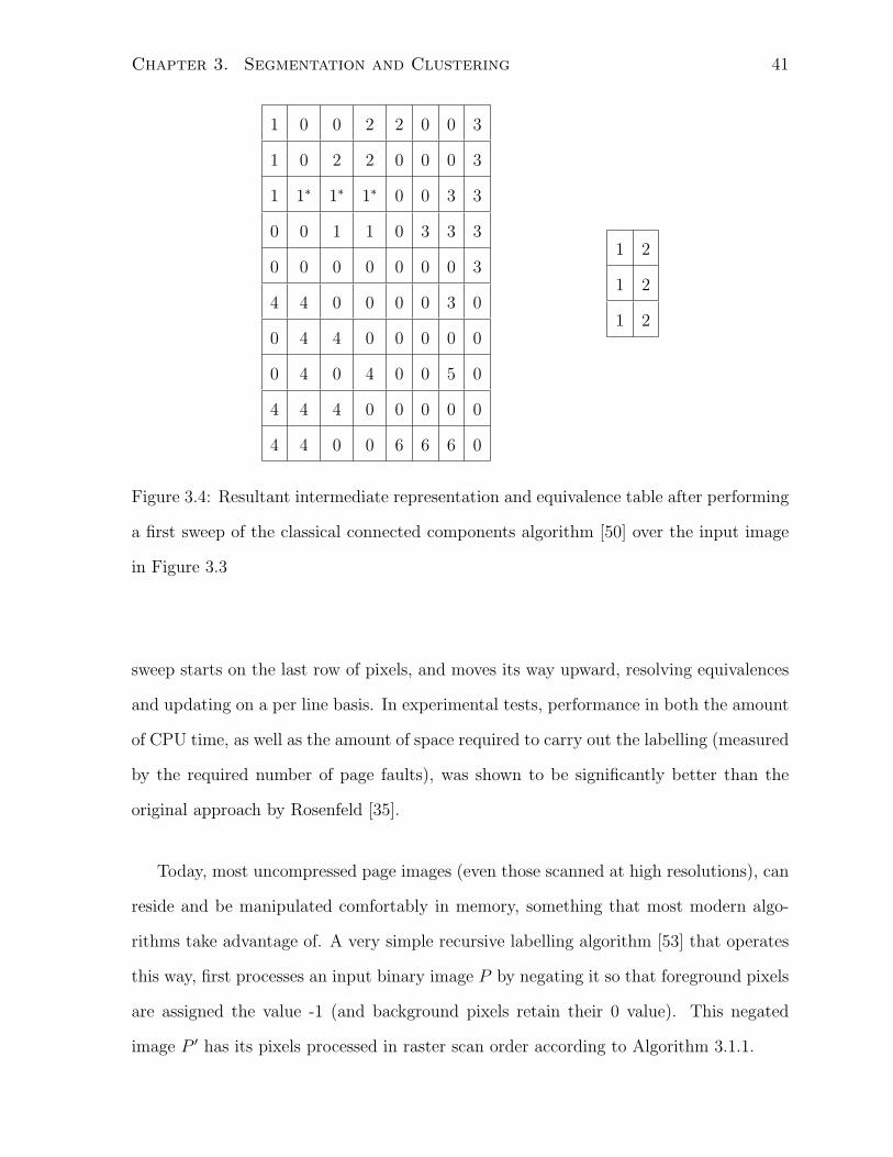
Chapter 3. Segmentation and Clustering 41
1 0 0 2 2 0 0 3
1 0 2 2 0 0 0 3
1 1∗ 1∗ 1∗ 0 0 3 3
0 0 1 1 0 3 3 3
0 0 0 0 0 0 0 3
4 4 0 0 0 0 3 0
0 4 4 0 0 0 0 0
0 4 0 4 0 0 5 0
4 4 4 0 0 0 0 0
4 4 0 0 6 6 6 0
1 2
1 2
1 2
Figure 3.4: Resultant intermediate representation and equivalence table after performing
a first sweep of the classical connected components algorithm [50] over the input image
in Figure 3.3
sweep starts on the last row of pixels, and moves its way upward, resolving equivalences
and updating on a per line basis. In experimental tests, performance in both the amount
of CPU time, as well as the amount of space required to carry out the labelling (measured
by the required number of page faults), was shown to be significantly better than the
original approach by Rosenfeld [35].
Today, most uncompressed page images (even those scanned at high resolutions), can
reside and be manipulated comfortably in memory, something that most modern algo-
rithms take advantage of. A very simple recursive labelling algorithm [53] that operates
this way, first processes an input binary image P by negating it so that foreground pixels
are assigned the value -1 (and background pixels retain their 0 value). This negated
image P ′ has its pixels processed in raster scan order according to Algorithm 3.1.1.
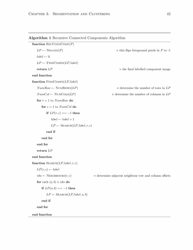
Chapter 3. Segmentation and Clustering 42
Algorithm 1 Recursive Connected Components Algorithm
function RecConnComp(P )
LP ← Negate(P ) . this flips foreground pixels in P to -1
label← 0
LP ← FindComps(LP, label)
return LP . the final labelled component image
end function
function FindComps(LP, label)
NumRow ← NumRows(LP ) . determine the number of rows in LP
NumCol← NumCols(LP ) . determine the number of columns in LP
for r = 1 to NumRow do
for c = 1 to NumCol do
if LP (r, c) == −1 then
label← label + 1
LP ← Search(LP, label, r, c)
end if
end for
end for
return LP
end function
function Search(LP, label, r, c)
LP (r, c)← label
nbs← Neighbours(r, c) . determine adjacent neighbour row and column offsets
for each (a, b) ∈ nbs do
if LP (a, b) == −1 then
LP ← Search(LP, label, a, b)
end if
end for
end function
Chapter 3. Segmentation and Clustering 43
3.1.2 Line Identification
Assuming that the input document image contains regions that are predominantly tex-
tual, it becomes beneficial to be able to discern the boundaries of each line of text. For
instance it can be a useful aid in skew correction or verification procedures, and it also
helps determine useful character properties like baseline and x-height offset. For lan-
guages with a left-to-right reading order, text lines are often long horizontal sections,
and the baseline defines the horizontal position that the bottom pixels of most symbols
just reach. Symbols that extend below this baseline offset are called descenders, and for
the Latin alphabet this includes symbols like y, j, p. The x-height is also a horizontal
line (for left-to-right reading languages), which indicates were the topmost pixels of a
majority of symbols lie. It is so named because the offset position represents the height
of a lower-case x symbol as measured from the baseline. Symbols that extend above the
x-height offset are called ascenders, and include Latin alphabet symbols like i, t, d as
well as all digit and upper-case character symbols. Not all text found in document images
is written in a strict left-to-right ordering. Many languages are read in a top-to-bottom
fashion, which results in vertical lines of text. For spatial or stylistic reasons, text lines
can be found oriented in arbitrary directions, making their identification quite trouble-
some. In the discussion that follows we restrict ourselves to methods that attempt to
find horizontal text lines, though first performing script and language recognition on a
document image (as is discussed in Chapter 4) could be used to determine the typical
text line orientation.
Text line identification can be thought of as a particular flavour of region detection,
and a lot of the page segmentation strategies can be used directly to determine individual
lines of text. For instance, by simply choosing a small enough vertical cut threshold, the
recursive XY-cuts procedure [39] should yield individual regions for each text line on most
well spaced textual documents. The docstrum approach by O’Gorman [43] can find text
lines by performing the transitive closure roughly along the skew angle estimated from
Chapter 3. Segmentation and Clustering 44
neighbouring connected components. Care must be taken when a document contains
multiple columns of text (like some technical articles or newspapers). In such cases if
the text in these columns is aligned, a single horizontal line can mistakenly be identified
instead of two separate lines that happen to be horizontally adjacent. Reading order
information from zoning and page layout (see Chapter 2), as well as horizontal whitespace
gap size can be used to ensure line boundaries are correctly identified.
3.1.3 Segmenting Symbols from Components
The issue of having more or fewer than one symbol image contained within a found
connected component bounding box must be resolved prior to character recognition to
ensure accurate results. Obviously this resolution process is dependent on the language
and subsequent alphabet of symbols present, but for the most part it requires updates
that both split individual components into two or more components, as well as merge
together the bounding boxes of multiple components into a single symbol image compo-
nent. Unless the document is extremely noisy or poorly spaced, this breaking apart of
multiple touching symbols belonging to the same connected component is only required
in the reading-order direction of the document (horizontal for Latin-based languages).
Splitting Fused Symbols
There have been many approaches to segmenting document images into individual sym-
bols, some of the earliest of which have attempted to exploit properties like the height
and width of typical characters [20]. Starting from the bounding boxes of connected com-
ponents, measuring their average width and looking for boxes that are significantly wider
than this mean value are often good indications of a multiple symbol component for doc-
uments written in a left-to-right reading order based language, particularly when written
using a fixed pitch font. Such a method breaks down when a document is written in a
variable width font containing tightly kerned touching symbols or ligatures like fi that

Chapter 3. Segmentation and Clustering 45
end up being narrower than single wide symbols like w. Several other early approaches to
isolated symbol segmentation did not start from connected components, instead choosing
to vertically sum the pixel values of identified lines of text looking for minimal values
indicating probable segmentation points [7] (see the example in Figure 3.5). When de-
termining whether or not to split apart a component containing multiple symbols in a
known language, Fujisawa et al [16] showed that the contours of the foreground pixels
can be followed to determine potential segmentation points. They tested their approach
against the segmentation of touching hand written numerals and found that 97% of the
time, the numerals end up joined in just one of three different patterns. If at least one
of two touching symbols contains a rounded contour at the join point, this can often be
identified by performing successive erosion operations on the pixel images [18] (though
it will fail if the joined symbols happen to touch along a straight line, such is often the
case with serif characters). Once an ideal set of segmentation points has been identified,
selecting the best among them can usually be accomplished by exploiting the fact that
most symbol images appear multiple times in a document. Each potential segmentation
can be tried in turn, and the pieces that result from that segmentation can be searched
for matching images among the rest of the components. While a ligature like fi will of-
ten result in a single fused component, other pairs of characters like fr or in are usually
separated into separate components allowing one to split the ligature and find matches
among individual f and i components.
Figure 3.5: Fused connected component, with horizontal and vertical projection profiles
shown, as well as potential segmentation points found by minimal projection profile
Chapter 3. Segmentation and Clustering 46
Merging Broken Symbols
Identifying and merging components containing only parts of a symbol is complementary
to solving the problem of splitting fused symbols above. A lot of the same properties
can be used to determine when two or more connected components should be merged.
The merger process is highly language and alphabet dependent. As will be discussed in
Section 3.4.1, for the English language, several symbols composed of multiple connected
components can typically be recombined based on their horizontal overlap and vertical
proximity. Broken symbols are particularly common in hand printed text as the writer
constantly picks up the pen between strokes, leading to small gaps between parts of
symbols. Poor scanner quality coupled with too high of a binarization threshold can
fragment symbols. Shridhar and Badreldin [54] found that for hand printed numerals,
these broken symbols could often be found by following contour pixels and looking for
horizontal or vertical discontinuities (though this approach will not work if starting from
a connected components representation). Another simple approach involves looking for
connected components that lie close to one another, then determine if this temporarily
joined component happens to match another component in shape, size, and line-offset.
The computation time required to carry out this check can become quite large, and
care must be taken to ensure that two separate symbols are not accidentally merged.
For example when considering separate components c and l under certain tightly spaced
fonts, this can often look very similar to the single symbol d, though these symbols should
not be merged in such a case. Shape information alone is not sufficient to determine
whether a merger should be made in such a case, instead the segmentation decision may
have to come after, or as part of the recognition process.
Recognition Based Segmentation
More recent research has highlighted the strong interconnectedness of character segmen-
tation and recognition processes such that many segmentation strategies actually depend
Chapter 3. Segmentation and Clustering 47
on an initial character recognition score to guide which components should be further
split and re-segmented [38]. Such procedures can iterate between the two tasks, perform-
ing classification on an initial sequence of connected components, then those components
with low scores are searched for potential split points (or merges with neighbouring low
scoring components), updated, and reclassified.
Instead of calculating connected components, Lecun et al [31] took words and lines
of input text, and proceeded to oversegment them into many pieces with each potential
segmentation point representing a node in a directed, acyclic graph. Edges are drawn
between these nodes to generate several possible segmentation scenarios (each valid path
through this graph defines a single segmentation of the word or line of text). The best
such segmentation is found via the Viterbi decoding algorithm [15], where the cost along
each edge (which represents some portion of pixels from the line), is determined by the
recognition score assigned by a trained convolutional neural network.
Holistic Methods
Holistic methods attempt to bypass the issue of finding a suitable character segmentation
by considering words as the atomic units of recognition [7]. These methods exploit the
fact that for documents written in languages whose atomic symbols represent phonemes
or portions of words, the space between these atomic symbols may be small enough
that some of them end up touching, but the spacing between groups of these symbols
representing the words are almost always separated by a recognizable gap. Thus each
word can be identified as one or more connected component, alleviating the problem of
having to identify and locate suitable split points in the components. A major downside to
this approach is the explosion in the size of the alphabet since distinct atomic “symbols”
now represent words instead of isolated characters. As a result, the use of holistic methods
is typically employed when the vocabulary is of a small, fixed length (like a cheque reader
designed to read numerical amount strings or dates).
Chapter 3. Segmentation and Clustering 48
3.2 Clustering Components
After preprocessing and the determination of a reasonable set of lines and connected
components has been carried out on each page of the document image, the next step
involves grouping or clustering these components together. This clustering serves two
major purposes. First, if done in such a manner that each component represents a single
symbol and only components representing the same symbol end up in each cluster, then
recognition of the entire document boils down to recognition of the single symbol in each
cluster (since the label determined for a single cluster can then be applied to all of its
elements). Secondly, an accurate clustering allows one to determine statistical properties
and features of the symbols that appear in the document to be recognized. Counts based
on how frequently each type of symbol is seen, as well as a sense of what symbols tend
to follow what other symbols can be taken. This information forms the backbone of our
contextual approach to character recognition, so the precision with which components
can be clustered goes a long way in shaping the overall accuracy of our recognizer.
The clustering of arbitrary objects can proceed in one of two ways. In partition
based approaches all the objects are grouped during a single pass, whereas in hierarchical
approaches, the set of clusters produced at each stage is a result of refining the clusters
determined in a previous stage. Hierarchical clustering approaches are further categorized
depending on whether they work in a divisive or agglomerative fashion. In divisive or
top-down clustering, each object is initially assigned to the same cluster, and at each step
the objects determined to lie farthest (based on some sort of comparison metric that can
be determined for each object), are removed from the original cluster, and placed into
new clusters. This procedure typically repeats until either the desired number of clusters
has been reached, or the differences between the objects falls below the threshold used
to separate them, and so no further changes are possible. In contrast, agglomerative or
bottom-up clustering procedures start with each object assigned to its own cluster. At
each step, objects are compared and those found to lie closest to one another (based
Chapter 3. Segmentation and Clustering 49
on some distance criterion) are merged together under the same cluster. Again, this
procedure repeats until the desired number of clusters has been found, or no objects lie
close enough to be merged into other clusters. Hierarchical clustering approaches can be
represented by a tree structure often called a dendrogram. Divisive clustering starts at
the root and works its way down the tree, whereas agglomerative clustering starts at the
leaves, and works its way upward toward the root. In both cases, the tree may be cut
before the leaves (or the root respectively) are reached.
3.2.1 Distance Metrics Used for Cluster Comparison
Clustering objects together requires that they be grouped based on some measure of
similarity. An object belonging to a particular cluster should be more “similar” to each
of the other objects belonging to that cluster, than to any of the objects belonging to any
other cluster. When working with image representations of symbols from an alphabet,
this notion of similarity should attempt to group all instances of a particular symbol
together in the same cluster, without including any instances of another symbol. Since
each symbol image is represented by a matrix of pixel intensity values located by the
co-ordinates of its rectangular bounding box, similarity should be calculated using this
information in some manner. Often, this is carried out by converting the m row by
n column matrix representation into a single vector of pixels of length m × n. These
vectors can then be thought of as defining points in an m × n dimensional Euclidean
space, where each pixel’s value contributes to the final point location along a single
dimension. By representing each symbol image as a point in Euclidean space, this allows
us to determine similarity of two images based on the distance between their defined
points. Many methods for calculating this distance exist, and we briefly introduce a few
of which that we happen to make use of in our implementation.
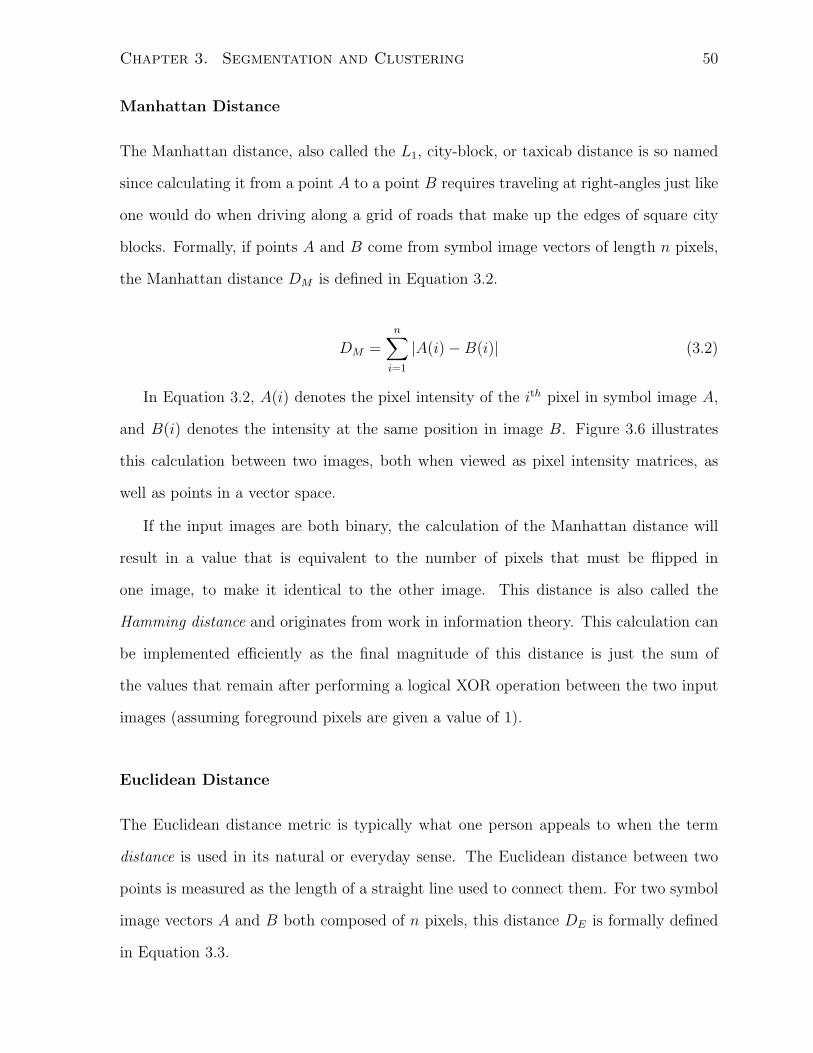
Chapter 3. Segmentation and Clustering 50
Manhattan Distance
The Manhattan distance, also called the L1, city-block, or taxicab distance is so named
since calculating it from a point A to a point B requires traveling at right-angles just like
one would do when driving along a grid of roads that make up the edges of square city
blocks. Formally, if points A and B come from symbol image vectors of length n pixels,
the Manhattan distance DM is defined in Equation 3.2.
DM =n∑
i=1
|A(i)−B(i)| (3.2)
In Equation 3.2, A(i) denotes the pixel intensity of the ith pixel in symbol image A,
and B(i) denotes the intensity at the same position in image B. Figure 3.6 illustrates
this calculation between two images, both when viewed as pixel intensity matrices, as
well as points in a vector space.
If the input images are both binary, the calculation of the Manhattan distance will
result in a value that is equivalent to the number of pixels that must be flipped in
one image, to make it identical to the other image. This distance is also called the
Hamming distance and originates from work in information theory. This calculation can
be implemented efficiently as the final magnitude of this distance is just the sum of
the values that remain after performing a logical XOR operation between the two input
images (assuming foreground pixels are given a value of 1).
Euclidean Distance
The Euclidean distance metric is typically what one person appeals to when the term
distance is used in its natural or everyday sense. The Euclidean distance between two
points is measured as the length of a straight line used to connect them. For two symbol
image vectors A and B both composed of n pixels, this distance DE is formally defined
in Equation 3.3.
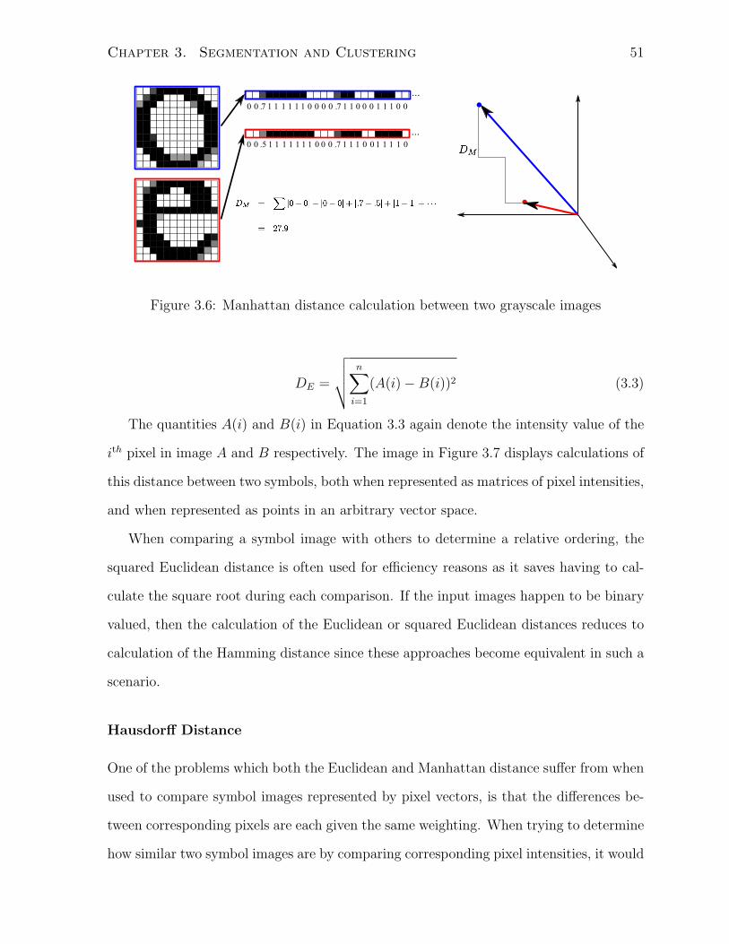
Chapter 3. Segmentation and Clustering 51
Figure 3.6: Manhattan distance calculation between two grayscale images
DE =
√√√√ n∑i=1
(A(i)−B(i))2 (3.3)
The quantities A(i) and B(i) in Equation 3.3 again denote the intensity value of the
ith pixel in image A and B respectively. The image in Figure 3.7 displays calculations of
this distance between two symbols, both when represented as matrices of pixel intensities,
and when represented as points in an arbitrary vector space.
When comparing a symbol image with others to determine a relative ordering, the
squared Euclidean distance is often used for efficiency reasons as it saves having to cal-
culate the square root during each comparison. If the input images happen to be binary
valued, then the calculation of the Euclidean or squared Euclidean distances reduces to
calculation of the Hamming distance since these approaches become equivalent in such a
scenario.
Hausdorff Distance
One of the problems which both the Euclidean and Manhattan distance suffer from when
used to compare symbol images represented by pixel vectors, is that the differences be-
tween corresponding pixels are each given the same weighting. When trying to determine
how similar two symbol images are by comparing corresponding pixel intensities, it would
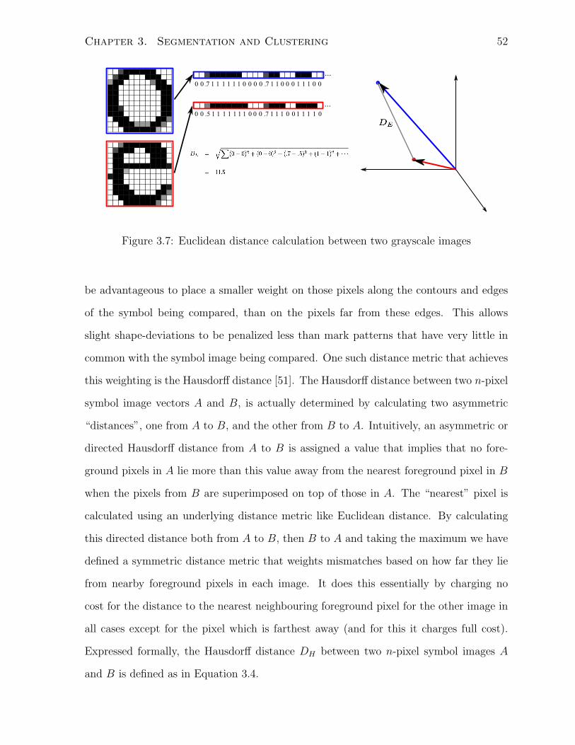
Chapter 3. Segmentation and Clustering 52
Figure 3.7: Euclidean distance calculation between two grayscale images
be advantageous to place a smaller weight on those pixels along the contours and edges
of the symbol being compared, than on the pixels far from these edges. This allows
slight shape-deviations to be penalized less than mark patterns that have very little in
common with the symbol image being compared. One such distance metric that achieves
this weighting is the Hausdorff distance [51]. The Hausdorff distance between two n-pixel
symbol image vectors A and B, is actually determined by calculating two asymmetric
“distances”, one from A to B, and the other from B to A. Intuitively, an asymmetric or
directed Hausdorff distance from A to B is assigned a value that implies that no fore-
ground pixels in A lie more than this value away from the nearest foreground pixel in B
when the pixels from B are superimposed on top of those in A. The “nearest” pixel is
calculated using an underlying distance metric like Euclidean distance. By calculating
this directed distance both from A to B, then B to A and taking the maximum we have
defined a symmetric distance metric that weights mismatches based on how far they lie
from nearby foreground pixels in each image. It does this essentially by charging no
cost for the distance to the nearest neighbouring foreground pixel for the other image in
all cases except for the pixel which is farthest away (and for this it charges full cost).
Expressed formally, the Hausdorff distance DH between two n-pixel symbol images A
and B is defined as in Equation 3.4.
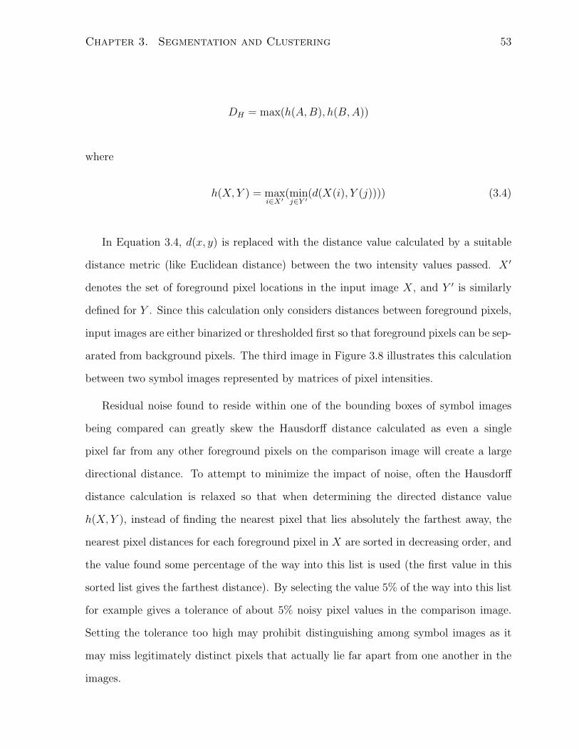
Chapter 3. Segmentation and Clustering 53
DH = max(h(A, B), h(B, A))
where
h(X, Y ) = maxi∈X′
(minj∈Y ′
(d(X(i), Y (j)))) (3.4)
In Equation 3.4, d(x, y) is replaced with the distance value calculated by a suitable
distance metric (like Euclidean distance) between the two intensity values passed. X ′
denotes the set of foreground pixel locations in the input image X, and Y ′ is similarly
defined for Y . Since this calculation only considers distances between foreground pixels,
input images are either binarized or thresholded first so that foreground pixels can be sep-
arated from background pixels. The third image in Figure 3.8 illustrates this calculation
between two symbol images represented by matrices of pixel intensities.
Residual noise found to reside within one of the bounding boxes of symbol images
being compared can greatly skew the Hausdorff distance calculated as even a single
pixel far from any other foreground pixels on the comparison image will create a large
directional distance. To attempt to minimize the impact of noise, often the Hausdorff
distance calculation is relaxed so that when determining the directed distance value
h(X, Y ), instead of finding the nearest pixel that lies absolutely the farthest away, the
nearest pixel distances for each foreground pixel in X are sorted in decreasing order, and
the value found some percentage of the way into this list is used (the first value in this
sorted list gives the farthest distance). By selecting the value 5% of the way into this list
for example gives a tolerance of about 5% noisy pixel values in the comparison image.
Setting the tolerance too high may prohibit distinguishing among symbol images as it
may miss legitimately distinct pixels that actually lie far apart from one another in the
images.
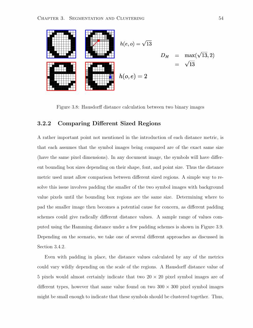
Chapter 3. Segmentation and Clustering 54
Figure 3.8: Hausdorff distance calculation between two binary images
3.2.2 Comparing Different Sized Regions
A rather important point not mentioned in the introduction of each distance metric, is
that each assumes that the symbol images being compared are of the exact same size
(have the same pixel dimensions). In any document image, the symbols will have differ-
ent bounding box sizes depending on their shape, font, and point size. Thus the distance
metric used must allow comparison between different sized regions. A simple way to re-
solve this issue involves padding the smaller of the two symbol images with background
value pixels until the bounding box regions are the same size. Determining where to
pad the smaller image then becomes a potential cause for concern, as different padding
schemes could give radically different distance values. A sample range of values com-
puted using the Hamming distance under a few padding schemes is shown in Figure 3.9.
Depending on the scenario, we take one of several different approaches as discussed in
Section 3.4.2.
Even with padding in place, the distance values calculated by any of the metrics
could vary wildly depending on the scale of the regions. A Hausdorff distance value of
5 pixels would almost certainly indicate that two 20 × 20 pixel symbol images are of
different types, however that same value found on two 300 × 300 pixel symbol images
might be small enough to indicate that these symbols should be clustered together. Thus,
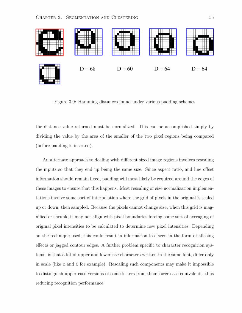
Chapter 3. Segmentation and Clustering 55
Figure 3.9: Hamming distances found under various padding schemes
the distance value returned must be normalized. This can be accomplished simply by
dividing the value by the area of the smaller of the two pixel regions being compared
(before padding is inserted).
An alternate approach to dealing with different sized image regions involves rescaling
the inputs so that they end up being the same size. Since aspect ratio, and line offset
information should remain fixed, padding will most likely be required around the edges of
these images to ensure that this happens. Most rescaling or size normalization implemen-
tations involve some sort of interpolation where the grid of pixels in the original is scaled
up or down, then sampled. Because the pixels cannot change size, when this grid is mag-
nified or shrunk, it may not align with pixel boundaries forcing some sort of averaging of
original pixel intensities to be calculated to determine new pixel intensities. Depending
on the technique used, this could result in information loss seen in the form of aliasing
effects or jagged contour edges. A further problem specific to character recognition sys-
tems, is that a lot of upper and lowercase characters written in the same font, differ only
in scale (like c and C for example). Rescaling such components may make it impossible
to distinguish upper-case versions of some letters from their lower-case equivalents, thus
reducing recognition performance.
Chapter 3. Segmentation and Clustering 56
3.3 Addition of Word-Space Demarcations
In order to carry out our contextual recognition approach over phoneme-based languages,
it becomes important to be able to accurately demarcate word boundaries. This can
be accomplished by estimating the inter-word space width, then looking for connected
components whose nearest neighbour distance exceeds this width.
Figure 3.10 displays a histogram showing the horizontal pixel distance frequency
between nearest neighbour components after clustering a 15 page document scanned
at 196dpi (the fine-mode fax compressed letter 9460 from the ISRI legal letter dataset
[42] was used). As this figure illustrates, this distribution is typically bimodal with
the first peak near the average inter-character space width, and the second smaller and
flatter peak near the average inter-word space width. The range in character and word
space values can be attributed to the variable width font used, as well as different space
widths employed to kern characters and ensure that the text in each paragraph remains
fully justified. To accurately determine where words begin and end we must attempt
to automatically estimate a suitable position in the valley between these two peaks.
Since each document will generate different histograms based on its input resolution and
content, a principled method must be employed to determine this inter-character cut-off
value.
One such principled approach introduced by Huang et al [25] models these histogram
widths as a mixture of 2 Poisson distributions. After calculating the set of horizontal
space widths s1, . . . sN between neighbouring components, parameters representing the
threshold c at which a space width should be considered an inter-word space (as opposed
to inter-character), as well as the rate parameters λ1, λ2 for the inter-character and inter-
word Poisson distributions are estimated. Each space width si is modelled according to
the probability in Equation 3.5
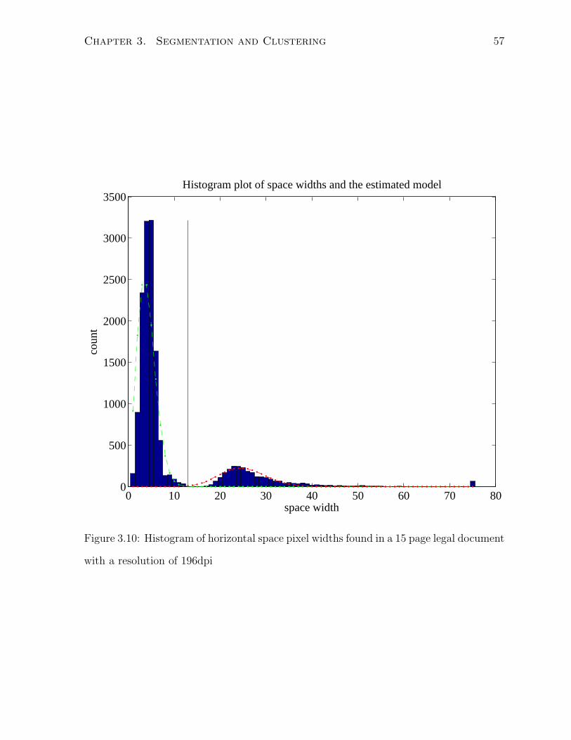
Chapter 3. Segmentation and Clustering 57
0 10 20 30 40 50 60 70 800
500
1000
1500
2000
2500
3000
3500Histogram plot of space widths and the estimated model
space width
coun
t
Figure 3.10: Histogram of horizontal space pixel widths found in a 15 page legal document
with a resolution of 196dpi
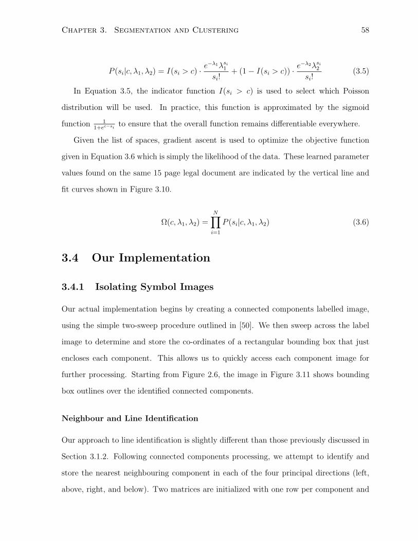
Chapter 3. Segmentation and Clustering 58
P (si|c, λ1, λ2) = I(si > c) · e−λ1λsi
1
si!+ (1− I(si > c)) · e
−λ2λsi2
si!(3.5)
In Equation 3.5, the indicator function I(si > c) is used to select which Poisson
distribution will be used. In practice, this function is approximated by the sigmoid
function 11+ec−si
to ensure that the overall function remains differentiable everywhere.
Given the list of spaces, gradient ascent is used to optimize the objective function
given in Equation 3.6 which is simply the likelihood of the data. These learned parameter
values found on the same 15 page legal document are indicated by the vertical line and
fit curves shown in Figure 3.10.
Ω(c, λ1, λ2) =N∏
i=1
P (si|c, λ1, λ2) (3.6)
3.4 Our Implementation
3.4.1 Isolating Symbol Images
Our actual implementation begins by creating a connected components labelled image,
using the simple two-sweep procedure outlined in [50]. We then sweep across the label
image to determine and store the co-ordinates of a rectangular bounding box that just
encloses each component. This allows us to quickly access each component image for
further processing. Starting from Figure 2.6, the image in Figure 3.11 shows bounding
box outlines over the identified connected components.
Neighbour and Line Identification
Our approach to line identification is slightly different than those previously discussed in
Section 3.1.2. Following connected components processing, we attempt to identify and
store the nearest neighbouring component in each of the four principal directions (left,
above, right, and below). Two matrices are initialized with one row per component and
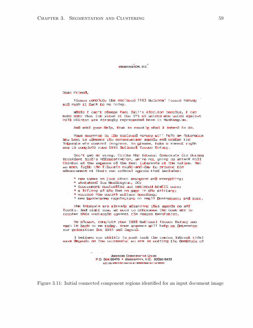
Chapter 3. Segmentation and Clustering 59
Figure 3.11: Initial connected component regions identified for an input document image
Chapter 3. Segmentation and Clustering 60
four columns. The first will store the label of the nearest component in each direction
(using a dummy label of 0 if no such neighbour exists in that direction), and the second
matrix stores the pixel distance to that neighbouring component (using a value of ∞ if
no neighbour is present in that direction). The first matrix is initialized to 0 everywhere,
and the second to ∞ everywhere. The foreground pixels of the document image are
first scanned from top to bottom along each row, before moving on to the adjacent
column. The connected component label li of the first seen foreground pixel is stored,
and compared with the next foreground pixel found in that column. If it belongs to
a different component lj then the distance d between these two pixels is compared to
determine if either matrix should be updated. For li, if the entry for its row and below
neighbour column is a 0 in the first matrix, or is a value larger than d in the second matrix,
then lj represents the new closest below neighbour to li. The matrices are updated so
that for li’s below neighbour column, the first matrix has a value lj, and the second has
a value d. Similarly, for lj, its above neighbour column is checked and if either its label
value is 0, or its distance value is larger than d, then it gets updated with a values of li and
d respectively. The current foreground pixel gets updated to lj and this process repeats
over each transition. It also repeats over each column until the entire document image
has been processed, and final nearest above and below neighbour labels and distances
have been estimated for each component. A second analogous pass is then employed to
calculate left and right nearest neighbour components and distances, but this time the
scanning is done left to right across each column before exploring an adjacent row. To
ensure multiple column page layouts are handled correctly, this left to right exploration
follows the reading order determined as part of the region detection process in Chapter 2.
Thus at any given time we only explore columns based on the currently identified region
we are attempting to identify left and right neighbours of.
Armed with this nearest neighbour information, we find text lines by first scanning
component bounding box co-ordinate positions to find the component that lies closest

Chapter 3. Segmentation and Clustering 61
to the top of the page. For multiple column pages, we actually restrict the search to
within the column currently being identified. We then follow left neighbours of this
component until we find a component with no left neighbour listed (this component
becomes our initial line anchor). The first line region bounding box is initialized to the
co-ordinates of the anchor component, then right neighbours are followed starting from
the anchor. At each step we potentially update the top, right, and bottom line boundary
co-ordinates so that this new component is completely covered. We also attempt to
follow left neighbours of the bottom neighbour of the component most recently added to
the line. If this left-most component happens to match our original anchor component,
then the co-ordinates of the line boundary are updated to ensure they encompass each
of the bottom and left neighbours explored along the sequence. If they do not match,
this different left neighbour has its co-ordinates compared to see if it should be marked
as the next line anchor to start from. This will happen if it lies closer to the top than
any other explored left-most neighbour. During this exploration checks are made to
ensure that we do not end up seeing the same component twice (which can occur if one
component lies completely or partially inside another). If this occurs neighbours and
distances are updated to remove this cycle. This process then repeats moving one step
to the right, updating line boundary co-ordinates and checking the bottom neighbour’s
left-most neighbour, until we reach a component with no right neighbour. At this point
we consider this line complete, associate its line number with each component that has
been seen to lie within its bounding box and repeat on the closest next anchor point.
After this procedure is complete, a reasonable list of lines (for a single column) will
have been found. As a final cleanup step, we search for any remaining components not
found to belong to a particular line number (but that lie within the current column being
processed), then if its co-ordinates completely or partially lie within a single line region,
the line region boundaries are extended appropriately and this component is added. If
a component happens to cross two or more line boundaries, then they are merged to a
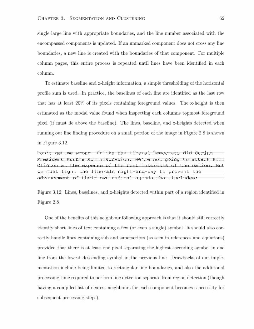
Chapter 3. Segmentation and Clustering 62
single large line with appropriate boundaries, and the line number associated with the
encompassed components is updated. If an unmarked component does not cross any line
boundaries, a new line is created with the boundaries of that component. For multiple
column pages, this entire process is repeated until lines have been identified in each
column.
To estimate baseline and x-height information, a simple thresholding of the horizontal
profile sum is used. In practice, the baselines of each line are identified as the last row
that has at least 20% of its pixels containing foreground values. The x-height is then
estimated as the modal value found when inspecting each columns topmost foreground
pixel (it must lie above the baseline). The lines, baseline, and x-heights detected when
running our line finding procedure on a small portion of the image in Figure 2.8 is shown
in Figure 3.12.
Figure 3.12: Lines, baselines, and x-heights detected within part of a region identified in
Figure 2.8
One of the benefits of this neighbour following approach is that it should still correctly
identify short lines of text containing a few (or even a single) symbol. It should also cor-
rectly handle lines containing sub and superscripts (as seen in references and equations)
provided that there is at least one pixel separating the highest ascending symbol in one
line from the lowest descending symbol in the previous line. Drawbacks of our imple-
mentation include being limited to rectangular line boundaries, and also the additional
processing time required to perform line detection separate from region detection (though
having a compiled list of nearest neighbours for each component becomes a necessity for
subsequent processing steps).

Chapter 3. Segmentation and Clustering 63
Diacritic Merging
As can be seen by the image in Figure 3.11, the result of running connected components
labelling does not always yield isolated character bounding boxes. Broken or fragmented
individual symbols can appear spread over multiple components for a number of rea-
sons, including a symbol actually consisting of more than one connected grouping of
pixels, or because noise or a poor choice of binarization thresholds has split the symbol.
For Latin-based alphabets, we employ a simple yet effective approach to merging frag-
mented components that belong to the same symbol. Using the line information found
in Section 3.1.2, we attempt to merge vertically split components (almost all multiple
component symbols in Latin alphabets are separated vertically with the double quote
symbol " being a notable exception). We merge two such components provided that they
belong to the same line (are contained within the same line boundary), have bounding
boxes separated by no more than a threshold of x pixels (where the threshold is small
and set based on the input document resolution), and have one of the components com-
pletely overlapping the other horizontally. Figure 3.13 shows the updated bounding boxes
that result in performing this merging procedure on one region of the original connected
component sample found in Figure 3.11
Figure 3.13: Updated connected components found for a small region after a vertical
merging procedure has occurred
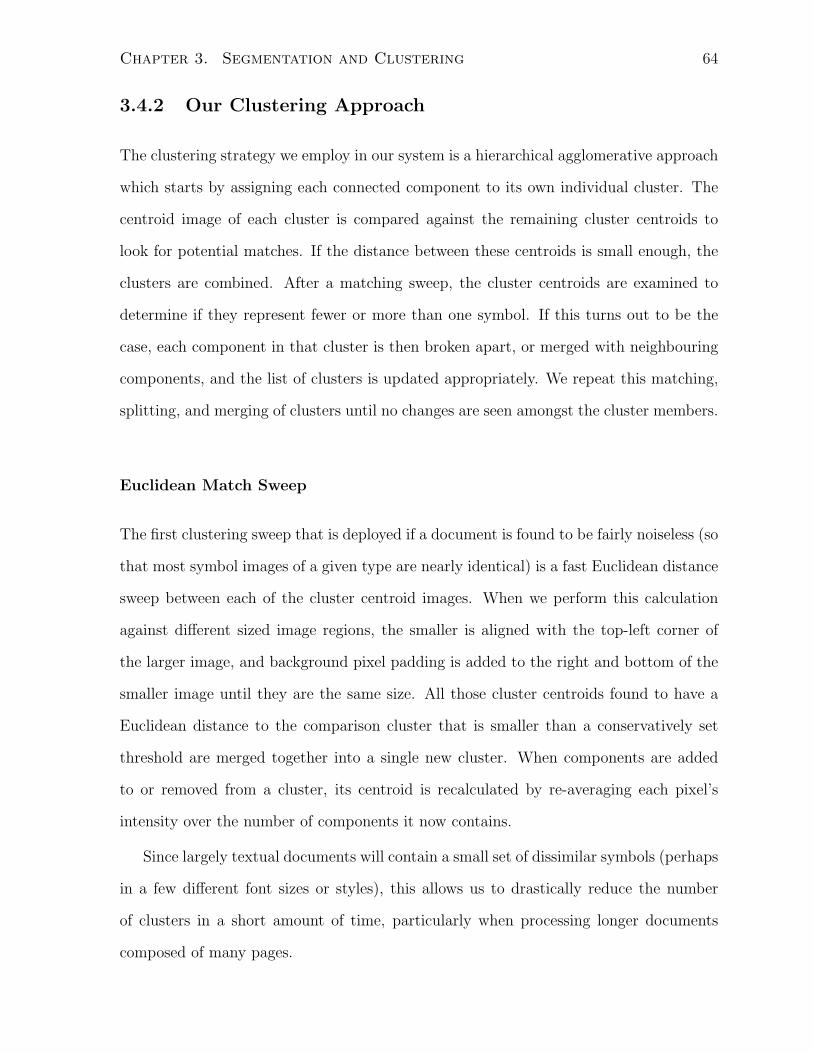
Chapter 3. Segmentation and Clustering 64
3.4.2 Our Clustering Approach
The clustering strategy we employ in our system is a hierarchical agglomerative approach
which starts by assigning each connected component to its own individual cluster. The
centroid image of each cluster is compared against the remaining cluster centroids to
look for potential matches. If the distance between these centroids is small enough, the
clusters are combined. After a matching sweep, the cluster centroids are examined to
determine if they represent fewer or more than one symbol. If this turns out to be the
case, each component in that cluster is then broken apart, or merged with neighbouring
components, and the list of clusters is updated appropriately. We repeat this matching,
splitting, and merging of clusters until no changes are seen amongst the cluster members.
Euclidean Match Sweep
The first clustering sweep that is deployed if a document is found to be fairly noiseless (so
that most symbol images of a given type are nearly identical) is a fast Euclidean distance
sweep between each of the cluster centroid images. When we perform this calculation
against different sized image regions, the smaller is aligned with the top-left corner of
the larger image, and background pixel padding is added to the right and bottom of the
smaller image until they are the same size. All those cluster centroids found to have a
Euclidean distance to the comparison cluster that is smaller than a conservatively set
threshold are merged together into a single new cluster. When components are added
to or removed from a cluster, its centroid is recalculated by re-averaging each pixel’s
intensity over the number of components it now contains.
Since largely textual documents will contain a small set of dissimilar symbols (perhaps
in a few different font sizes or styles), this allows us to drastically reduce the number
of clusters in a short amount of time, particularly when processing longer documents
composed of many pages.
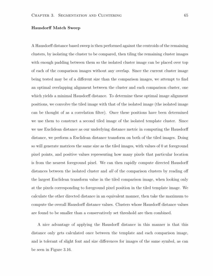
Chapter 3. Segmentation and Clustering 65
Hausdorff Match Sweep
A Hausdorff distance based sweep is then performed against the centroids of the remaining
clusters, by isolating the cluster to be compared, then tiling the remaining cluster images
with enough padding between them so the isolated cluster image can be placed over top
of each of the comparison images without any overlap. Since the current cluster image
being tested may be of a different size than the comparison images, we attempt to find
an optimal overlapping alignment between the cluster and each comparison cluster, one
which yields a minimal Hausdorff distance. To determine these optimal image alignment
positions, we convolve the tiled image with that of the isolated image (the isolated image
can be thought of as a correlation filter). Once these positions have been determined
we use them to construct a second tiled image of the isolated template cluster. Since
we use Euclidean distance as our underlying distance metric in computing the Hausdorff
distance, we perform a Euclidean distance transform on both of the tiled images. Doing
so will generate matrices the same size as the tiled images, with values of 0 at foreground
pixel points, and positive values representing how many pixels that particular location
is from the nearest foreground pixel. We can then rapidly compute directed Hausdorff
distances between the isolated cluster and all of the comparison clusters by reading off
the largest Euclidean transform value in the tiled comparison image, when looking only
at the pixels corresponding to foreground pixel position in the tiled template image. We
calculate the other directed distance in an equivalent manner, then take the maximum to
compute the overall Hausdorff distance values. Clusters whose Hausdorff distance values
are found to be smaller than a conservatively set threshold are then combined.
A nice advantage of applying the Hausdorff distance in this manner is that this
distance only gets calculated once between the template and each comparison image,
and is tolerant of slight font and size differences for images of the same symbol, as can
be seen in Figure 3.16.
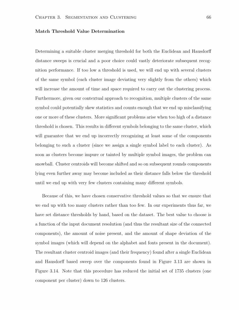
Chapter 3. Segmentation and Clustering 66
Match Threshold Value Determination
Determining a suitable cluster merging threshold for both the Euclidean and Hausdorff
distance sweeps is crucial and a poor choice could vastly deteriorate subsequent recog-
nition performance. If too low a threshold is used, we will end up with several clusters
of the same symbol (each cluster image deviating very slightly from the others) which
will increase the amount of time and space required to carry out the clustering process.
Furthermore, given our contextual approach to recognition, multiple clusters of the same
symbol could potentially skew statistics and counts enough that we end up misclassifying
one or more of these clusters. More significant problems arise when too high of a distance
threshold is chosen. This results in different symbols belonging to the same cluster, which
will guarantee that we end up incorrectly recognizing at least some of the components
belonging to such a cluster (since we assign a single symbol label to each cluster). As
soon as clusters become impure or tainted by multiple symbol images, the problem can
snowball. Cluster centroids will become shifted and so on subsequent rounds components
lying even further away may become included as their distance falls below the threshold
until we end up with very few clusters containing many different symbols.
Because of this, we have chosen conservative threshold values so that we ensure that
we end up with too many clusters rather than too few. In our experiments thus far, we
have set distance thresholds by hand, based on the dataset. The best value to choose is
a function of the input document resolution (and thus the resultant size of the connected
components), the amount of noise present, and the amount of shape deviation of the
symbol images (which will depend on the alphabet and fonts present in the document).
The resultant cluster centroid images (and their frequency) found after a single Euclidean
and Hausdorff based sweep over the components found in Figure 3.13 are shown in
Figure 3.14. Note that this procedure has reduced the initial set of 1735 clusters (one
component per cluster) down to 126 clusters.
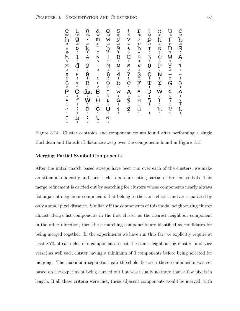
Chapter 3. Segmentation and Clustering 67
Figure 3.14: Cluster centroids and component counts found after performing a single
Euclidean and Hausdorff distance sweep over the components found in Figure 3.13
Merging Partial Symbol Components
After the initial match based sweeps have been run over each of the clusters, we make
an attempt to identify and correct clusters representing partial or broken symbols. This
merge refinement is carried out by searching for clusters whose components nearly always
list adjacent neighbour components that belong to the same cluster and are separated by
only a small pixel distance. Similarly if the components of this modal neighbouring cluster
almost always list components in the first cluster as the nearest neighbour component
in the other direction, then these matching components are identified as candidates for
being merged together. In the experiments we have run thus far, we explicitly require at
least 85% of each cluster’s components to list the same neighbouring cluster (and vice
versa) as well each cluster having a minimum of 3 components before being selected for
merging. The maximum separation gap threshold between these components was set
based on the experiment being carried out but was usually no more than a few pixels in
length. If all these criteria were met, these adjacent components would be merged, with

Chapter 3. Segmentation and Clustering 68
their bounding boxes and neighbours updated and either the clusters themselves would
be merged to a single cluster (if all components matched), or the existing cluster(s) were
kept if they had at least one element that did not match, with a new cluster created to
hold the matching components.
Splitting Multiple Symbol Components
To attempt to split apart components that contain more than one symbol joined hori-
zontally, each cluster centroid is scanned for potential cut points based on its projection
profile and width. At each reasonable point found, the image is temporarily split, and
matches of each half of the image are searched for among the remaining cluster images
(recursively segmenting the right half at appropriate points if necessary). The Hausdorff
distance is usually computed between these temporary splits and the rest of the clusters,
and a suitable threshold is set (usually given approximately the same value as for the
match threshold). If each half of the temporary segmentation matches a cluster with a
distance lower than this threshold, then the split is made at these cut points for each com-
ponent in this cluster, and each of the new components has its neighbours recalculated,
and is added to its matching cluster. The original cluster is removed.
Iterative Cluster Refinement
During each phase of attempted matching, merging, and splitting of the clusters, those
clusters that end up affected in some manner by these operations are marked for further
processing. Each of these marked clusters is then subjected to a subsequent round of
matches, mergers, and splits until no change is seen in cluster groupings. The final set
of cluster centroids (and their frequency) found when iteratively splitting, merging, and
matching the initial set of clusters found in Figure 3.14 is shown in Figure 3.15. Because
this particular input document contains very few split or merge segments, the final set of
cluster centroids only decreases by 3 from that found during the initial matching sweep.
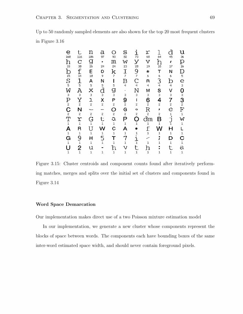
Chapter 3. Segmentation and Clustering 69
Up to 50 randomly sampled elements are also shown for the top 20 most frequent clusters
in Figure 3.16
Figure 3.15: Cluster centroids and component counts found after iteratively perform-
ing matches, merges and splits over the initial set of clusters and components found in
Figure 3.14
Word Space Demarcation
Our implementation makes direct use of a two Poisson mixture estimation model
In our implementation, we generate a new cluster whose components represent the
blocks of space between words. The components each have bounding boxes of the same
inter-word estimated space width, and should never contain foreground pixels.
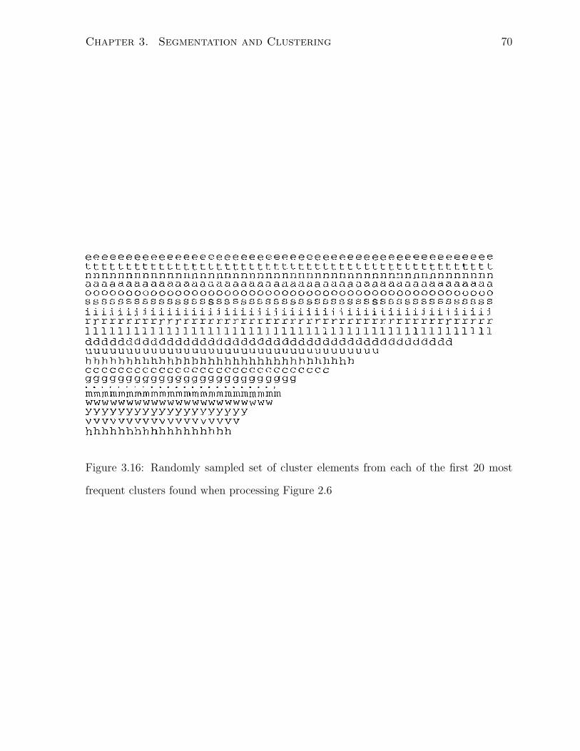
Chapter 3. Segmentation and Clustering 70
Figure 3.16: Randomly sampled set of cluster elements from each of the first 20 most
frequent clusters found when processing Figure 2.6
Chapter 4
Context-Based Symbol Recognition
In this chapter we outline our approach to the fundamental task of OCR systems, namely
the recognition and assignment of labels to each isolated symbol image. Most of the time,
these labels are numeric codes that represent entries in standardized symbol tables like
ASCII or Unicode1. In the simplest task where we do not aim to preserve layout infor-
mation, our goal is simply to determine the sequence of mappings in the “reading-order”
of the document (left to right, top to bottom for English) and thus reduce the origi-
nal input document image to an approximation that is understandable by a computer.
Depending on the software tools available and the user’s requirements, auxiliary region
information can be incorporated into the final output format. In many cases the final
recognized result ends up as a file formatted for word processing software, though in spe-
cial applications this output may instead be formatted for spreadsheet, Computer aided
design, sheet music, or other software packages. Graphs, line drawings, and other figures
typically remain as images in the final output. Some attempts may be made to process
and arrange tabular data, though this remains a difficult and active area of research [14].
The traditional approach to inferring the mapping from glyph images to labels pro-
ceeds in a bottom-up fashion. Once these images have been suitably isolated, the raw
1http://unicode.org
71
Chapter 4. Context-Based Symbol Recognition 72
pixel intensities or features taken from these pixel intensities are fed as input into some
sort of shape-based classifier, whose output is the predicted label for that image. Most
current systems are initially trained on a large and varied collection of font shapes so
that the system can recognize the characters in documents written in a wide array of font
faces. Depending on the features and implementation, such classifiers can sometimes suc-
cessfully generalize to untrained fonts, though this only works when the font face differs
by a minuscule amount from sample fonts used to initially train the classifier (see the
experimental results run on Figure 1.4 which are reported in Table 1.2). When faced with
novel input fonts that do not closely resemble any of the trained samples, shape-based
classifiers tend to perform very poorly (though humans have very little trouble distin-
guishing and recognizing such symbol images). This inability to generalize becomes an
increasing problem for shape-based classifiers, particularly as new software tools enable
ordinary users to design and create their own custom fonts2. As a result, the number
and variety of fonts seen in input document images continues to grow, motivating the
pursuit of alternate approaches to tackling the character recognition problem.
One way of guaranteeing that a recognition system will generalize to untrained or
unseen font faces and styles is to have the input document itself provide the font model.
Unless the document is a ransom note, page from a font manual, or extremely noisy,
each occurrence of a particular symbol glyph will remain relatively consistent everywhere
that symbol is used in the document (using multiple font faces and sizes could alter this,
though consistencies still exist). Our clustering approach described in Chapter 3 attempts
to exploit this idea, however the glyph shapes found remain unlabelled (unlike shape-
based classifiers which make use of labelled training samples). Determining the labels
or symbol mapping associated with each cluster requires that we appeal to information
not present in the cluster glyph shapes (since we would like our approach to remain font
neutral). Fortunately, several non shape-based sources of information exist. In particular,
2http://www.fontlab.com
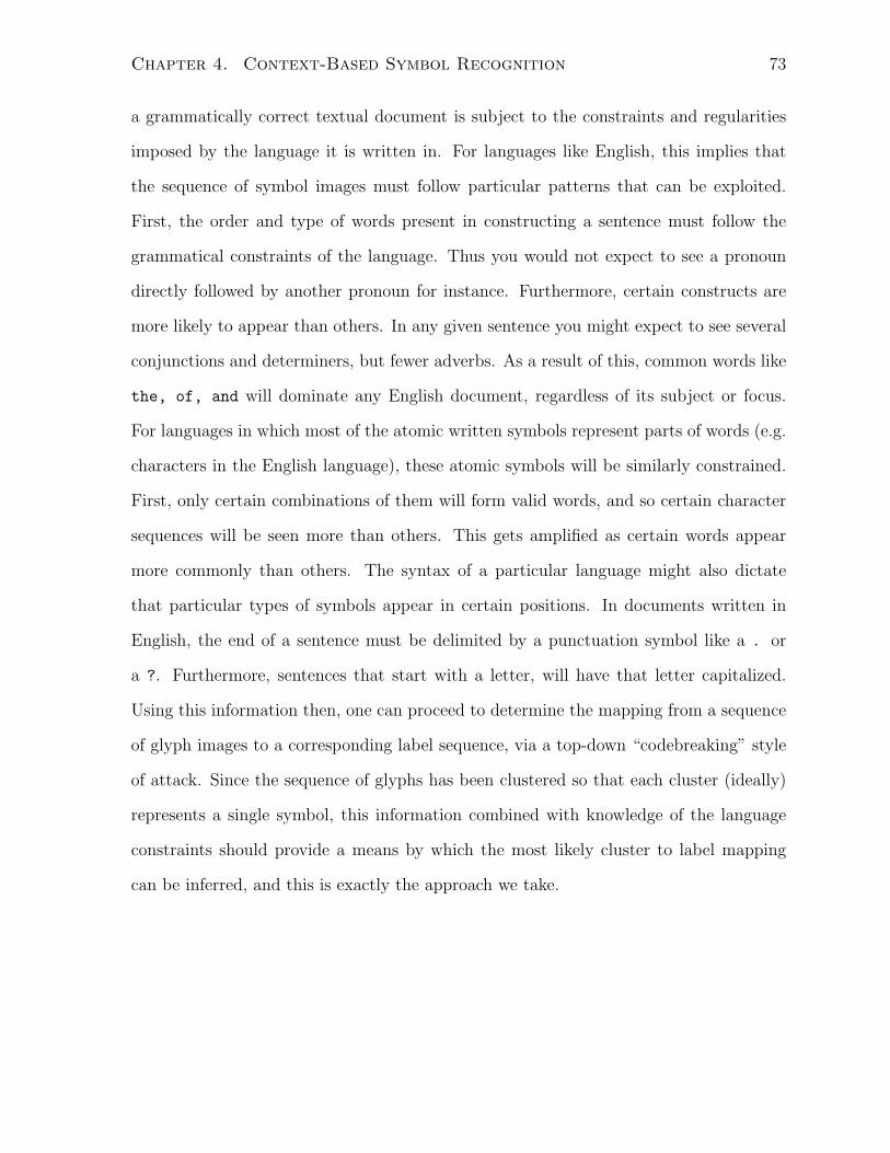
Chapter 4. Context-Based Symbol Recognition 73
a grammatically correct textual document is subject to the constraints and regularities
imposed by the language it is written in. For languages like English, this implies that
the sequence of symbol images must follow particular patterns that can be exploited.
First, the order and type of words present in constructing a sentence must follow the
grammatical constraints of the language. Thus you would not expect to see a pronoun
directly followed by another pronoun for instance. Furthermore, certain constructs are
more likely to appear than others. In any given sentence you might expect to see several
conjunctions and determiners, but fewer adverbs. As a result of this, common words like
the, of, and will dominate any English document, regardless of its subject or focus.
For languages in which most of the atomic written symbols represent parts of words (e.g.
characters in the English language), these atomic symbols will be similarly constrained.
First, only certain combinations of them will form valid words, and so certain character
sequences will be seen more than others. This gets amplified as certain words appear
more commonly than others. The syntax of a particular language might also dictate
that particular types of symbols appear in certain positions. In documents written in
English, the end of a sentence must be delimited by a punctuation symbol like a . or
a ?. Furthermore, sentences that start with a letter, will have that letter capitalized.
Using this information then, one can proceed to determine the mapping from a sequence
of glyph images to a corresponding label sequence, via a top-down “codebreaking” style
of attack. Since the sequence of glyphs has been clustered so that each cluster (ideally)
represents a single symbol, this information combined with knowledge of the language
constraints should provide a means by which the most likely cluster to label mapping
can be inferred, and this is exactly the approach we take.
Chapter 4. Context-Based Symbol Recognition 74
4.1 Script and Language Determination
Before we can begin to decode the clustered sequence of symbol images using language
constraints, we must obviously determine what language the document image is written
in. Choosing an incorrect language would certainly have catastrophic effects on recogni-
tion accuracy when a strongly contextual approach is used. While it would take minimal
effort to have the user select the input language prior to performing the OCR process,
it would be ideal if this could be automated so that no user intervention is required
(particularly if the recognition work is to be performed unattended on a large batch of
documents).
Fortunately, previous work has shown it largely possible to distinguish both the script
and underlying language of document images. Script refers to the set of alphanumeric and
punctuation symbols used in written versions of a language. Some scripts are unique to
individual languages (like the Hangul script is for Korean text), whereas others are shared
among several languages (like the Roman script for the English, French, Vietnamese, and
other languages).
Building off earlier work capable of distinguishing between 23 different Roman script
languages [55], Spitz extended this to incorporate several Han-based languages like Ko-
rean, Japanese and Chinese [56]. Input document images are first grouped into one of
two script classes by examining the distribution over the vertical offset position (rela-
tive to the baseline) at which upwardly concaving pixel intensities appear. For Roman
scripts, this distribution is largely bi-modal, with a large peak near the baseline and a
second peak near the x-height line. For Han-based scripts, this concave vertical offset
distribution is much more uniform, so the variance of these distributions can be used
to determine which group an input document belongs to. An example showing upward
concaving points (highlighted in a lighter colour) for both the English language as well
as a Han-based language is illustrated in Figure 4.1.
For documents belonging to the Han-based group, distinguishing between Chinese,
Chapter 4. Context-Based Symbol Recognition 75
Figure 4.1: Upward concavities found in small samples of Roman (left) and Han-based
scripts (right)
Japanese, and Korean documents is carried out by measuring the character density (inside
its rectangular bounding box). Chinese characters are generally more dense than Korean
or Japanese, so this provides a useful starting point. The distribution of these densities
is calculated and the area under these plots is integrated at three key regions. Linear
discriminant analysis is carried out on a small training set of labelled input documents
at these regions to determine two salient linear combinations that best separate these
inputs based on class. At test time, the same linear combinations are calculated on the
region areas of the density curve from the input document, and the document is classified
according to the training document which lies closest in terms of Euclidean distance in
this linearly combined input feature space.
Documents written in a Roman script are further classified into one of 23 languages
based on the frequency in which certain “word shape tokens” appear. Each word shape
token is composed of one or more “character shape codes”. Each symbol image is clas-
sified as one of six different character shape codes based on its number of connected
components, as well as where its components lie in relation to the baseline and x-height.
Those that ascend above the x-height line will generally be grouped in a different class
than those that descend below the baseline etc. Since each language will be composed of
many stop-words common to that language (words like the in English, der in German,
or le in French), the distribution over word shape tokens should show characteristically
distinct peaks, allowing one to determine the underlying language of an input Roman
script document.
A related approach carried out by Hochberg et al [23] was tested on languages written
Chapter 4. Context-Based Symbol Recognition 76
in 13 different scripts. Distinguishing between these scripts was determined by first
collecting and rescaling connected components found in training documents for each
language. These components were clustered together based on shape similarity, and the
average or centroid of each cluster was used as a template symbol for that language
(clusters with few components were removed). At test time, the script of an input
document was determined by normalizing found connected components and determining
how many matched trained templates from each script. The script which achieved the
best matching score was then selected for the input document. While this system has
the advantage of being easily deployed for arbitrary scripts, it was shown to be sensitive
to the fonts the documents were trained on. Thus even though an input document may
be in a trained script, if it is written in an untrained font, this approach may fail to
correctly determine its script.
4.2 Previous Top-Down Work
There have been several approaches to top-down or purely contextual character recog-
nition, a few of which are outlined and discussed here. Each of these methods either
assumes, or makes an initial attempt at grouping together similar shaped symbol images
(refer back to Chapter 3 for an examination of various image clustering approaches).
By assigning a unique identifier to each cluster found, we can then determine the resul-
tant sequence of these identifiers as shown in Figure 4.2. Furthermore, we can also use
the distance between neighbouring components to infer word boundaries in all but the
noisiest of input document images (typically these gaps are large enough that symbols
belonging to different words remain separated). The recognition task then boils down to
determining the mapping from each cluster identifier to its appropriate symbol label.
Inferring this mapping is equivalent to decoding a cryptogram: the input sequence
of cluster identifiers represents the encrypted ciphertext, and the unknown sequence of
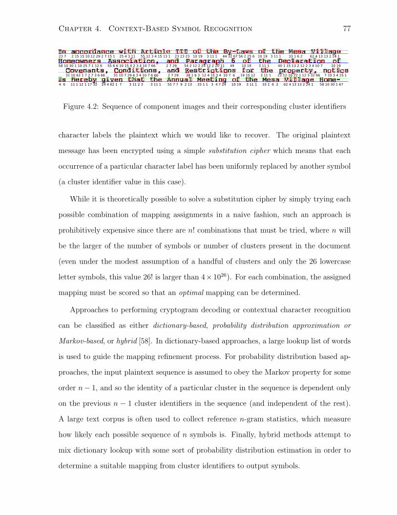
Chapter 4. Context-Based Symbol Recognition 77
Figure 4.2: Sequence of component images and their corresponding cluster identifiers
character labels the plaintext which we would like to recover. The original plaintext
message has been encrypted using a simple substitution cipher which means that each
occurrence of a particular character label has been uniformly replaced by another symbol
(a cluster identifier value in this case).
While it is theoretically possible to solve a substitution cipher by simply trying each
possible combination of mapping assignments in a naive fashion, such an approach is
prohibitively expensive since there are n! combinations that must be tried, where n will
be the larger of the number of symbols or number of clusters present in the document
(even under the modest assumption of a handful of clusters and only the 26 lowercase
letter symbols, this value 26! is larger than 4×1026). For each combination, the assigned
mapping must be scored so that an optimal mapping can be determined.
Approaches to performing cryptogram decoding or contextual character recognition
can be classified as either dictionary-based, probability distribution approximation or
Markov-based, or hybrid [58]. In dictionary-based approaches, a large lookup list of words
is used to guide the mapping refinement process. For probability distribution based ap-
proaches, the input plaintext sequence is assumed to obey the Markov property for some
order n− 1, and so the identity of a particular cluster in the sequence is dependent only
on the previous n − 1 cluster identifiers in the sequence (and independent of the rest).
A large text corpus is often used to collect reference n-gram statistics, which measure
how likely each possible sequence of n symbols is. Finally, hybrid methods attempt to
mix dictionary lookup with some sort of probability distribution estimation in order to
determine a suitable mapping from cluster identifiers to output symbols.
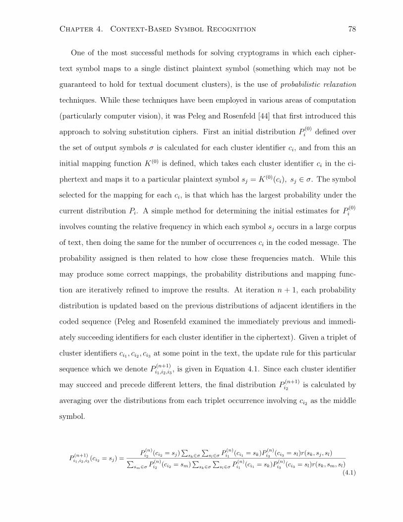
Chapter 4. Context-Based Symbol Recognition 78
One of the most successful methods for solving cryptograms in which each cipher-
text symbol maps to a single distinct plaintext symbol (something which may not be
guaranteed to hold for textual document clusters), is the use of probabilistic relaxation
techniques. While these techniques have been employed in various areas of computation
(particularly computer vision), it was Peleg and Rosenfeld [44] that first introduced this
approach to solving substitution ciphers. First an initial distribution P(0)i defined over
the set of output symbols σ is calculated for each cluster identifier ci, and from this an
initial mapping function K(0) is defined, which takes each cluster identifier ci in the ci-
phertext and maps it to a particular plaintext symbol sj = K(0)(ci), sj ∈ σ. The symbol
selected for the mapping for each ci, is that which has the largest probability under the
current distribution Pi. A simple method for determining the initial estimates for P(0)i
involves counting the relative frequency in which each symbol sj occurs in a large corpus
of text, then doing the same for the number of occurrences ci in the coded message. The
probability assigned is then related to how close these frequencies match. While this
may produce some correct mappings, the probability distributions and mapping func-
tion are iteratively refined to improve the results. At iteration n + 1, each probability
distribution is updated based on the previous distributions of adjacent identifiers in the
coded sequence (Peleg and Rosenfeld examined the immediately previous and immedi-
ately succeeding identifiers for each cluster identifier in the ciphertext). Given a triplet of
cluster identifiers ci1 , ci2 , ci3 at some point in the text, the update rule for this particular
sequence which we denote P(n+1)i1,i2,i3
, is given in Equation 4.1. Since each cluster identifier
may succeed and precede different letters, the final distribution P(n+1)i2
is calculated by
averaging over the distributions from each triplet occurrence involving ci2 as the middle
symbol.
P(n+1)i1,i2,i3
(ci2 = sj) =P
(n)i2
(ci2 = sj)∑
sk∈σ
∑sl∈σ P
(n)i1
(ci1 = sk)P (n)i3
(ci3 = sl)r(sk, sj , sl)∑sm∈σ P
(n)i2
(ci2 = sm)∑
sk∈σ
∑sl∈σ P
(n)i1
(ci1 = sk)P (n)i3
(ci3 = sl)r(sk, sm, sl)(4.1)
Chapter 4. Context-Based Symbol Recognition 79
The function r(a, b, c) in Equation 4.1 is calculated from unigram and trigram fre-
quency counts taken from a large text corpus. Specifically, the relative proportion of
appearances in which the symbol sequence abc appears, is divided by the relative propor-
tion of appearances of a multiplied by b multiplied by c (these values are precomputed
and stored for efficiency).
While the relaxation approach can not be guaranteed to converge to a particular op-
timal solution, in experiments run by Peleg and Rosenfeld using a 26 character symbol
alphabet over several short documents (including the Gettysburg address), nearly all the
symbols were correctly recovered after 10-15 iterations (they also introduced an alter-
nate update procedure that did not simply average individual distributions and found it
converged faster, but did not always perform as well).
In one of the earliest approaches designed specifically for OCR, Nagy et al [41],[40]
used a small lookup word dictionary written in the target language to aid in inferring the
mapping of identifiers to the appropriate lowercase character labels. Cluster sequence
words with the fewest unmapped symbols were first identified, then among those un-
mapped words, each unmapped symbol was ordered in a decreasing fashion based on
occurrence frequency. For each such symbol, a list of candidate labels was found based
on the number of matching dictionary words that appear when that label is replaced for
each occurrence of that symbol. The first symbol is temporarily mapped to the first can-
didate label, and this process repeats until either each symbol has been mapped, or the
number of completely mapped words that are not valid dictionary words exceeds some
threshold. In the latter case, mappings are unassigned until this score improves, then the
next candidate label is tried. This assignment and backtracking approach repeats until
a final mapping can be established. Some of the limitations of this approach include the
assumption of a one-to-one mapping from cluster identifiers to character labels, as well
as the restriction to lowercase letter labels only.

Chapter 4. Context-Based Symbol Recognition 80
Published at around the same time as Nagy et al, Casey also attempted to come up
with a dictionary-based, OCR specific decoding scheme [6]. Unlike the previous efforts,
this work made some attempts to deal with multiple clusters mapping to the same symbol,
as well as handle broken and touching clusters. In Casey’s approach, an initial partially
correct mapping is assumed and then used to create an initial word sequence called the
master sequence. Each master word is fed through a spell-checker to get a list of claimant
words that closely match the original. For each claimant word, the individual symbols
are processed in pairs and examined against the symbols in the master. By assigning
each claimant symbol an individual or pair of adjacent symbols in the master, checks are
made to ensure that at least one of each claimant pair matches the master. Claimant
words not meeting this requirement are thrown out, reducing the length of the claimant
word list associated with each master. Using this remaining list of claimant words and
their individual symbol to master symbol mappings, scores are generated for each cluster
identifier by counting the number of occurrences that an identifier is found to map to
a particular symbol or symbol pair in the claimant word list (each count is multiplied
by the length of the claimant word in which it appears). Those identifiers for which
only a single symbol matches are immediately assigned, then the claimant word list is
re-processed so that words not matching these assigned symbols are thrown out. This
process repeats until identifiers with more than one mapping symbol are all that remain.
In such a scenario the identifier with the largest difference between first and second
mapping scores is assigned the first mapping choice, and so on until each identifier has
been mapped. While it was claimed that accurate identification and fast convergence
could be accomplished, no empirical results were presented. Furthermore this approach
has a strong dependence on an initial partially correct mapping, which must be quite
good in order for this procedure to generate an initial list of claimant words that will
also include the correct word in its list of choices. To handle punctuation, digits and
non-dictionary words Casey suggests first identifying and stripping small punctuation
Chapter 4. Context-Based Symbol Recognition 81
symbols, then using an acceptance threshold to determine whether a word decoding
should be deemed valid (no details are presented on how either of these steps should be
carried out).
In an attempt to accommodate potential many-to-many mappings, Ho and Nagy
[21] combined a large dictionary with a sequence of ad-hoc modules to determine map-
pings from cluster identifiers to character labels. Potential mappings assigned under
each module were scored based on what the authors call a “v/p ratio”. This ratio mea-
sures the number of words in which the identifiers to be mapped appear, against the
number of those words that can be found in a dictionary (wildcards are used for the
labels of unmapped symbols during lookup). The first module takes the three most fre-
quently occurring cluster identifiers, and tries all possible triplet assignments using the
eight most commonly seen character labels (a, e, i, o, n, r, s, t). The assignment
which produces the highest v/p ratio score is then applied as the final mapping for these
three clusters. Other modules include looking for partially mapped words that match a
single dictionary word, as well as assignments that give a significantly larger v/p score
than other assignments of the same symbol, and swapping assigned symbols to boost v/p
score. In experimental trials on a set of short business letter faxes [42], they found that
on two-thirds of the pages, they could successfully identify almost 80% of the characters
that belonged to words which were also present in their lookup dictionary (performance
over all words in the document, including those containing digits or punctuation was
approximately 68%). Average performance on the remaining one-third of the documents
was around 20% and suffered from catastrophic errors early in the segmentation and
mapping process. The authors note a major problem with their approach is the inability
to handle non-character symbols like digits and punctuation symbols. In follow-up work
attempting to address this situation [22], Ho and Nagy set about trying to automatically
classify each symbol image as a digit, punctuation mark, uppercase, or lowercase char-
acter (without determining which specific symbol the image represented). Using a large

Chapter 4. Context-Based Symbol Recognition 82
text corpus as a training document, bi and trigram statistics were calculated for each
symbol label, and from these, 11 features were created. These included how frequently
each symbol appeared, how often it appeared at the start and end of words, the average
positional location within a word, as well as the average word-length in which it appears.
These features were suitably normalized and from their values, a simple nearest neigh-
bour classifier was built. At test time, each symbol was assigned the class of the training
point which was found to have the closest Euclidean distance (when compared in feature
space). For long test documents, treating the entire training set of documents as a single
large document gave identification rates above 99%. When tested on shorter documents,
the classifier was modified to collect and average n-gram statistics over each training doc-
ument separately, resulting in a classification accuracy of around 90% (which represents
an improvement over the 84% achievable by assigning every symbol to the lower case
character class).
An alternate approach making use of Hidden Markov Models (HMMs) was introduced
by Lee [32]. HMMs have been shown to be well suited to a variety of tasks involving
sequential data including speech recognition, financial prediction, and DNA alignment.
In this particular setup, the sequence of observed cluster identifiers is assumed to be
generated by traversing a set of underlying hidden states, each of which represents a par-
ticular character label. To completely specify this model, each hidden state is assigned
some prior probability representing its likelihood as being the first state seen. The tran-
sitional probability between each state is then estimated. In Lee’s implementation, a
basic first-order Markov model is assumed, so bigram transition probabilities represent-
ing the likelihood of moving to the next adjacent state given the current state are the
only estimates required. Finally, for each hidden state, a distribution over output cluster
identifiers is also required. This represents how likely we are to generate a particular
cluster identifier, given a particular hidden character label state. Lee used a large text
corpus to estimate both the start state, and state transition probabilities. To estimate
Chapter 4. Context-Based Symbol Recognition 83
the output cluster identifier probabilities for each hidden state, a specialized version of
the Expectation Maximization (EM) algorithm [10], known as the Baum-Welch algorithm
[3] was employed. Starting from an initial estimate of these output emission probabil-
ities, an initial set of underlying hidden states can be determined. Then using these
hidden states, new estimates for the most likely output probabilities can be found. This
procedure iterates until the likelihood of the output probabilities ceases to improve (or
the amount of improvement falls below some threshold). Efficient dynamic programming
procedures exist for estimating these hidden states given some set of output probabilities
and transition probabilities, and the EM algorithm is guaranteed to converge to some
(locally) optimal solution. With final estimates of these distributions, the most likely
mapping from cluster identifiers to character labels can be found using Viterbi decoding
[15]. Starting from the initial state probabilities, the cost of transitioning to each adjacent
character label state is multiplied by the probability of outputting the observed cluster
identifier at that state. The state transition that maximizes this overall probability is
stored, as is the probability value, and this repeats by examining all possible transitions
from this state, and so on. One of the nice properties of the HMM approach is that it can
be made somewhat tolerant of noisy mappings. Each label state generates a distribution
over possible output cluster identifiers, thus it is perfectly possible (given adjacent state
transition probabilities) for the state to emit a particular identifier at one point, then a
different identifier later on in the sequence. Similarly, it is also possible for more than one
hidden state to emit the same identifier at various points in the sequence. Lee tested both
one-to-one as well as noisy mappings and found that given sufficiently long sequences of
cluster identifiers (at least 1000 symbols), the correct sequence of hidden character labels
could be found with over 90% accuracy in the noisy case.
Recently, Huang et al [25] have taken an entropy based approach to inferring cluster
identifier to character label mappings. Initially, cluster identifier sequences representing
each of the individual words in the input document image are converted to numerization
Chapter 4. Context-Based Symbol Recognition 84
strings, as are a large collection of words taken from a text corpus. A numerization string
is calculated by assigning a value of 1 to the first symbol seen, 2 to the next distinct
symbol, 3 to the next and so on. Each occurrence of a particular symbol (whether it be
a cluster identifier or character label) is replaced uniformly with the same value, thus an
input string of identifiers of the form 4 3 10 10 5 3 1 9 would be mapped to 1 2 3 3
4 2 5 6 for instance. An initial cluster identifier to character label mapping is computed
by collecting all the words in the corpus that have the same numerization string as the
current cluster identifier sequence being mapped. For each cluster identifier, counts are
taken over the character labels that occur in the same positions as the identifier among
these collected word lists, and normalized to determine a distribution over symbols for
that cluster identifier and numerization string. Initial mappings are determined for each
cluster identifier by multiplying together these distributions over all words in which it
appears in the input document sequence, then taking the character label mapping which
has the largest value. The entropy of these initial assignments is used to guide the
refinement process. Cluster identifier mappings will have a low entropy precisely when
the distribution over character label scores is sharply peaked at the chosen label alone.
Those distributions that are more uniform (and thus have several words with labels that
map approximately as frequently as the chosen mapping), will have a high entropy. The
cluster identifier mappings are examined in increasing order of their entropies and at
each step the label producing the largest score is assigned to that identifier. For the
remaining unexamined mappings, their entropies are recalculated by removing words
from the corpus which are now incompatible with the current mapping. Thus if identifier
4 was assigned the label c, then the identifier 9 in the partially mapped sequence 4
9 o w, would have initially matching dictionary words like brow, snow, blow, glow,
grow, know, flow removed, leaving only the word crow as matching. Thus the entropy
over the mapping to cluster identifier 9, would be updated so that instead of being
roughly uniform across letters like l, r and n, it would now be sharply peaked at r
Chapter 4. Context-Based Symbol Recognition 85
alone. This process repeats until all cluster identifiers have been examined. To extend
their approach beyond an assumed one-to-one mapping between identifiers and labels,
Huang et al examine cluster identifiers that when mapped to character labels, occur more
frequently in words that are not found in a lookup dictionary than those that do. For
each such identifier, the “closest” dictionary word is found, where closeness is determined
by the number of character addition, deletion, and substitution operations required to
convert the original word into a dictionary word. By tabulating this closest mapping for
each such word, the most common label string substitution can be determined, and this
is what the identifier is then remapped to. When tested against 314 pages of the UNLV
Department of Energy dataset [42], average character recognition performance was found
to be about 74% (though this improves to about 78% when considering lowercase letter
performance alone). Like many of the previous approaches, the implementation by Huang
et al fails to handle upper case letters, digits, or punctuation symbols. Their approach
may also suffer when the same symbol appears in multiple clusters. For example if the
second e symbol in the word even is assigned a different cluster identifier than the first,
this sequence will be given a numerization string 1 2 3 4 instead of the correct 1 2 1
3. As a result, the matching lexicon word list will be significantly different which could
end up altering the symbol predicted for the second e cluster (or the others in that
word). This is particularly true if the cluster only appears at a few places in the original
sequence.
4.3 New Approaches
In this section we introduce several new, purely contextual or cryptogram decoding based
recognition approaches, each of which attempts to exploit all of the available sources of
linguistic information present in textual documents. Though much of the discussion
that follows will assume the input documents are written in the English language, it
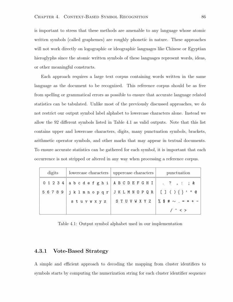
Chapter 4. Context-Based Symbol Recognition 86
is important to stress that these methods are amenable to any language whose atomic
written symbols (called graphemes) are roughly phonetic in nature. These approaches
will not work directly on logographic or ideographic languages like Chinese or Egyptian
hieroglyphs since the atomic written symbols of these languages represent words, ideas,
or other meaningful constructs.
Each approach requires a large text corpus containing words written in the same
language as the document to be recognized. This reference corpus should be as free
from spelling or grammatical errors as possible to ensure that accurate language related
statistics can be tabulated. Unlike most of the previously discussed approaches, we do
not restrict our output symbol label alphabet to lowercase characters alone. Instead we
allow the 92 different symbols listed in Table 4.1 as valid outputs. Note that this list
contains upper and lowercase characters, digits, many punctuation symbols, brackets,
arithmetic operator symbols, and other marks that may appear in textual documents.
To ensure accurate statistics can be gathered for each symbol, it is important that each
occurrence is not stripped or altered in any way when processing a reference corpus.
digits lowercase characters uppercase characters punctuation
0 1 2 3 4 a b c d e f g h i A B C D E F G H I . ? , : ; &
5 6 7 8 9 j k l m n o p q r J K L M N O P Q R [ ] ( ) ’ " @
s t u v w x y z S T U V W X Y Z % $ # ∼ = * + -
/ ^ < >
Table 4.1: Output symbol alphabet used in our implementation
4.3.1 Vote-Based Strategy
A simple and efficient approach to decoding the mapping from cluster identifiers to
symbols starts by computing the numerization string for each cluster identifier sequence

Chapter 4. Context-Based Symbol Recognition 87
(just as is done in [25]). The words of a large text corpus are similarly parsed. For
each cluster identifier, each of the words in which it appears has its corresponding list
of numerization string equivalent words selected, and votes are tallied for each symbol
that appears at the same position as the cluster identifier within the cluster sequence
word. If a cluster identifier happens to appear in multiple positions within a single
cluster sequence word, each lexicon matching word must also contain the same symbol
in the same positions. Determining the mapping for a particular identifier then involves
selecting the output symbol which is found to have the most votes.
In implementing this strategy, there are many decisions and choices to be made re-
garding how the votes are normalized as well as tabulated, and whether the matching
word lists are updated as cluster identifiers get mapped to symbols. We defer detailed
discussion regarding these choices to the experimental results of Section 5.3, where we
describe and report recognition accuracy over a wide variety of vote-based implementa-
tions.
4.3.2 Within-Word Positional Count Strategy
In this approach, each potential character or symbol label has positional statistics calcu-
lated for it based on where and how often it occurs within words in the corpus. Counts of
the number of times a symbol occurs within each possible position in words up to length
x are calculated, resulting in a feature vector of length x(x+1)2
. Similarly, these positional
counts are also estimated for each cluster identifier found in the input document to be
recognized. Since these feature vectors can equivalently be thought of as points in an
x(x+1)2
dimensional feature space, distances between them can be calculated and used to
define a measure of similarity or relatedness among such points. By comparing cluster
identifier positional features with symbol features estimated from a large corpus, it is
hoped that a suitable mapping from clusters to labels can be established.
An example illustrating the positional count vectors and corresponding distances
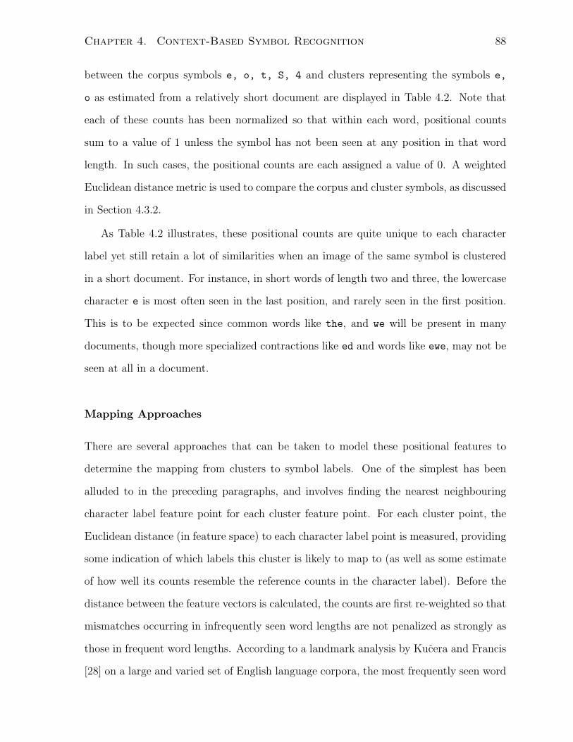
Chapter 4. Context-Based Symbol Recognition 88
between the corpus symbols e, o, t, S, 4 and clusters representing the symbols e,
o as estimated from a relatively short document are displayed in Table 4.2. Note that
each of these counts has been normalized so that within each word, positional counts
sum to a value of 1 unless the symbol has not been seen at any position in that word
length. In such cases, the positional counts are each assigned a value of 0. A weighted
Euclidean distance metric is used to compare the corpus and cluster symbols, as discussed
in Section 4.3.2.
As Table 4.2 illustrates, these positional counts are quite unique to each character
label yet still retain a lot of similarities when an image of the same symbol is clustered
in a short document. For instance, in short words of length two and three, the lowercase
character e is most often seen in the last position, and rarely seen in the first position.
This is to be expected since common words like the, and we will be present in many
documents, though more specialized contractions like ed and words like ewe, may not be
seen at all in a document.
Mapping Approaches
There are several approaches that can be taken to model these positional features to
determine the mapping from clusters to symbol labels. One of the simplest has been
alluded to in the preceding paragraphs, and involves finding the nearest neighbouring
character label feature point for each cluster feature point. For each cluster point, the
Euclidean distance (in feature space) to each character label point is measured, providing
some indication of which labels this cluster is likely to map to (as well as some estimate
of how well its counts resemble the reference counts in the character label). Before the
distance between the feature vectors is calculated, the counts are first re-weighted so that
mismatches occurring in infrequently seen word lengths are not penalized as strongly as
those in frequent word lengths. According to a landmark analysis by Kucera and Francis
[28] on a large and varied set of English language corpora, the most frequently seen word
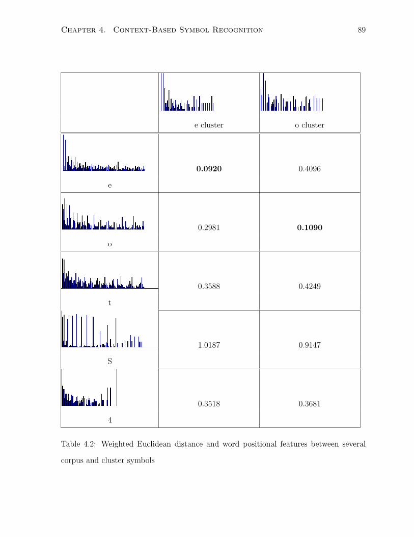
Chapter 4. Context-Based Symbol Recognition 89
e cluster o cluster
0.0920 0.4096
e
0.2981 0.1090
o
0.3588 0.4249
t
1.0187 0.9147
S
0.3518 0.3681
4
Table 4.2: Weighted Euclidean distance and word positional features between several
corpus and cluster symbols
Chapter 4. Context-Based Symbol Recognition 90
length was three characters, followed by two characters then four characters. It was also
found that over 81% of the words found in the corpora were of length 10 or less, and
98% were of length 15 or less. When calculated by taking into account the number of
occurrences of each word, more than 84% of the total corpus consisted of words of length
7 or less. Histograms of word length occurrence as found in the text corpus are used
to determine how much weight to apply to positional count differences for each word
length. In the simplest re-weighting approach, these weights are applied to all symbol
labels uniformly. Sample distances found when comparing several corpus symbols to two
different clusters using this simple re-weighting approach can be found in Table 4.2. In
our experiments, we also carried out tests by counting the frequency of each label in
each word length so that specific word length weighting factors for each reference symbol
could be employed (see Section 5.4).
Instead of classifying clusters based on their weighted Euclidean distance to symbols
(an approach that can be thought of as maximizing the likelihood of the mapping from
clusters to symbols), an alternate approach involves minimizing the cross entropy between
clusters and symbols. This approach requires first normalizing the positional counts so
that they define valid probability distributions. One method for doing so is to simply
take each cluster or symbol and divide each of its positional counts by the total number
of counts found over all positions and word lengths for that cluster or symbol. From
these distributions, the Kullback-Leibler (or KL) divergence can be calculated between
a particular cluster and each symbol. Letting P define the distribution over cluster
positional counts and Q the distribution over a particular symbol’s positional counts,
the value of this calculation can be found in Equation 4.2, where the discrete index i
will range over each of the x(x+1)2
word positions (assuming words up to length x are
included).
DKL(P ||Q) =∑
i
P (i) logP (i)
Q(i)(4.2)
Chapter 4. Context-Based Symbol Recognition 91
The KL divergence will yield a non-negative value which measures the relative entropy
between the cluster positional distribution and the corresponding symbol distribution.
Such a value can be loosely interpreted to represent the extra number of bits that must be
transmitted in a message describing the positional statistics of the cluster, when starting
from a description of the positional statistics of a particular symbol. The KL divergence
is 0 precisely when both sets of statistics are identical (since if they are identical, no
additional bits are required to transmit the cluster’s positional statistics). By calculating
the KL divergence between a cluster and each symbol, an estimate of which symbols
more “closely match” the cluster can be found, where closeness is defined as having a
minimal cross entropy value.
4.3.3 Cross-Word Constraint Strategy
A limitation of both the vote based, and positional statistic decoding approaches is that
neither makes use of constraints present across words in the document (that is, both op-
erate on each cluster sequence word independently). As a hypothetical example, consider
the cluster identifier words 10 1 4 3 and 1 5 19 7 2, and furthermore assume that the
mappings 4 → l, 5 → h, 19 → o, 7 → s, 2 → t are all known and correct (and that
each identifier represents exactly one symbol). Thus the first cluster sequence represents
a word of the form * * l * (the * symbols represent wildcards that are currently un-
known), and there are over 400 words in the English language that match such a pattern:
milk, wolf, solo, silk, sell, golf, cold, etc. The second cluster word is of the
form * h o s t and has only a single valid dictionary match, namely the word ghost.
Knowing the constraint that cluster identifier 1 must map to symbol g allows the list of
dictionary words matching the first cluster sequence to be significantly reduced to just
two potential matches: ugly and ogle.
Following this idea, our cross-word constraint strategy begins by first determining
the numerization strings of each cluster sequence word, as well as each word in the
Chapter 4. Context-Based Symbol Recognition 92
lexicon. Using these strings, an initial list of candidate matching words can be found
for each cluster sequence word. The process for generating this matching between lists
is not limited to those lexicon words that exactly match the cluster words numerization
strings. Instead, the requirement is relaxed so that any positions in which the cluster word
lists identical numerization values, words in the lexicon must list the same symbol value.
Distinct numerization values in the cluster word are free to map either to distinct symbols,
or the same symbol. This increases the initial number of matches, and ensures that cases
where multiple cluster identifiers map to the same symbol are handled appropriately. As
an example, if the cluster sequence representing the word e v e n has been coded so
that each e ends up in a different cluster (resulting in a numerization string of 1 2 3 4),
when looking for lexicon words that match, not only will we consider those of the form
1 2 3 4, but we will also include words of the form 1 2 1 3, 1 2 1 2, 1 1 2 2, etc.
After carrying out this process, any cluster words that have no candidates are marked as
invalid, and removed from further processing. Any cluster identifiers that always appear
mapped to the same value (and only that value) are considered correctly mapped, and
are substituted into cluster words to further reduce the list of matching lexicon words.
Starting from the most frequently occurring unmapped symbol, and the cluster word
containing that symbol that has the fewest matching lexicon words, we then record the
symbols that each of the cluster identifiers in this word can map to. If any cluster contains
0 valid mapping words, this word is marked as invalid, and the procedure continues on
to the next word containing the most frequent cluster and the fewest remaining lexicon
matches. Otherwise, the cluster word belonging to one of the cluster identifiers found in
the first word and containing the fewest matching lexicon symbols is sought and checks
are made to ensure that all pairwise cluster identifier constraints are satisfied across
these two word lists. This process repeats until either a unique mapping can be found
for a particular cluster identifier, or no valid mappings can be found, in which case the
first word is flagged as invalid. We continuously add a new word, check for mutual
Chapter 4. Context-Based Symbol Recognition 93
satisfaction across our current word list, and update matching lexicon words as more
clusters are mapped, until eventually we have mapped each cluster.
4.4 Additional Extensions
In this section we briefly introduce and discuss a couple of additional extensions that
can be applied to some of the new top-down recognition strategies in order to boost
recognition performance.
4.4.1 Explicit Dictionary Lookup
For some of the infrequently appearing clusters, each of the previously discussed mapping
approaches may yield an incorrectly assigned symbol. This is particularly true for the
positional statistic based approach as few appearances can severely skew these statistics
so that they lie farther away from the correct reference mapping than other incorrect label
points. To try and remedy such a situation, an initial set of mappings can be combined
with a large word list or dictionary. In our experiments, we simply extract the unique
words from our text corpus. We select clusters in order (starting with the most frequently
seen), and attempt to infer an improved label mapping using the initially found cluster
to label mappings and the lookup dictionary as guides. We extract the set of all cluster
identifier words in which the cluster being mapped appears at least once, and replace
already mapped identifiers in these words with their found character or symbol label. The
remaining unmapped identifiers appearing in these words are treated as wildcards. Each
potential label mapping is temporarily assigned to the cluster identifier currently under
consideration, and these partially mapped cluster words are searched for matching valid
dictionary words. Matches are considered valid when there is at least one dictionary word
that has the same length as the cluster word, and each mapped symbol in the cluster
word has the same label value and position in the lookup word (wildcards in the cluster
Chapter 4. Context-Based Symbol Recognition 94
word are considered capable of matching any symbol label). To better identify upper
case characters and punctuation, if the identifier appears in the first position of a word,
the lexicon words that begin with a lowercase letter are copied, but the first character is
replaced with its uppercase equivalent symbol. Similarly, if the identifier being mapped
appears in the last position of a cluster word, each lexicon word that is one symbol
shorter and does not end with a punctuation symbol is copied, and each of several valid
punctuation symbols are added to the end of these words, and each such word is added
to the dictionary. Under each temporary cluster identifier to character label mapping,
the ratio of the number of valid matching dictionary words, to total cluster words in
which the cluster identifier appears is calculated, and if this ratio exceeds a particular
threshold, then the mapping is considered valid and permanently assigned. The next
most frequently occurring cluster identifier is then found, and the process repeats.
Initially when there are very few (or no) mappings, most of the words in which the
cluster appears, will be considered valid dictionary words. Fortunately, if using the
positional statistical frequency mapping to get an initial ordering, the most frequently
occurring clusters are also the most likely to have positional statistics closely representing
those of the corresponding label in the reference corpus (simply because these symbols
are seen so frequently). Thus for the early assignments, the initial map ordering will
dominate which label is selected for each cluster, allowing us to bootstrap the recognition
process. Because these early symbols occur most frequently, they will quickly constrain
a majority of the cluster words, allowing the dictionary lookup ratios to successfully
identify the best mapping among less frequently occurring clusters (those for which an
initial mapping based on positional statistics are of less import).
Eventually, this recognition approach may reach a point where multiple symbols ex-
hibit the same dictionary lookup ratio. Breaking ties in such a scenario can be accom-
plished in a number of ways; the simplest of which involves choosing the label that comes
first based on the initially generated map ordering. This same approach can also be
Chapter 4. Context-Based Symbol Recognition 95
used when none of the mappings produce a lookup ratio above the desired threshold. An
alternate approach may make use of weak shape information in the form of baseline and
x-height offset. The set of symbols found to produce the same score can potentially be
reduced by considering only those symbols that have similar offsets as the cluster. This
information is largely font independent (i.e. regardless of the font, a lowercase g symbol
will almost always be seen to descend below the baseline by some amount).
4.4.2 Re-segmentation Refinement
Determining the mapping from cluster identifiers to symbols works optimally when each
identifier represents exactly one symbol. Due to noise or other complications, the clus-
tering process may leave multiple symbols fused together into a single element, or it may
break apart a symbol so that it becomes spread over several elements (and thus clus-
ters). Just as most modern shape-based recognition approaches make use of contextual
information to either improve an existing segmentation, or guide the current segmen-
tation [13] (also see Section 3.1.3), a top-down contextual recognition approach can be
used equivalently. Given an initial recognition, cluster identifiers that tend to appear
in words not found in a lookup dictionary can be flagged as candidates for potential re-
segmentation. Once split or merged, this new sequence of identifiers can either be passed
directly through a dictionary lookup to see if there is an improvement in the number of
matching words, or any of the initial mapping strategies like positional features can be
re-estimated and again checked to see if overall recognition accuracy improves.
Since merged cluster elements typically involve at most a few symbols, an alternate
approach would be to extend the symbol alphabet to include pairs or even triplets of
symbols before proceeding with the designed mapping strategy. While this may increase
computational costs, it may prevent having to perform a re-segmentation refinement.
Chapter 5
Experimental Results
In this chapter, we test each of our proposed clustering and top-down recognition ap-
proaches to OCR against several different datasets. Our goal is to assess recognition
performance on real-world data under a variety of scenarios by altering most aspects of
the input document images. This includes (but is not limited to) their length, quality,
orientation, contained symbols, subject matter or domain, layout, fonts, and appearance
of non-textual regions.
5.1 Experimental Setup
The majority of our tests were run against a set of short business letters, and a set
of long legal documents, both of which were taken from datasets produced by UNLV’s
Information Science Research Institute (ISRI)1 and will henceforth be denoted B and
L respectively [42]. All 159 documents from the B dataset (which were 1-2 pages in
length, and averaged 2010 symbols per document) were tested, as were the 10 longest
documents from the L dataset (which were numbered 9460-9469, were 15 pages in length,
and averaged 22,959 symbols per document). Using these datasets has several advantages,
1http://www.isri.unlv.edu
96
Chapter 5. Experimental Results 97
including the availability of ground truth zone and text information, as well as being
widely used in annual OCR system performance comparisons run throughout the mid-
1990’s [48]. The document images contained in these datasets represent real-world inputs,
and vary widely from one to the next. Both Figure 1.5 and Figure 2.5 show sample
input documents taken from this collection. Several different resolutions of each input
document are available, ranging from compressed 196 dpi fine-mode fax quality up to
400 dpi (all inputs are formatted as TIFF images).
Because our recognition approaches require the ability to perform tasks like dictio-
nary word lookup, issue votes for words matching a particular numerization string, and
estimate reference positional statistics, a large text corpus written in the language being
recognized is required. The Reuters-21578 text news corpus was chosen [34] for several
reasons. First, since the dataset consists of relatively short newswire articles, it will con-
tain many proper nouns, contractions and other words common to the English language
that would not generally appear in a dictionary. Punctuation, digit strings, and other non
alphabetic character symbols like brackets are also present throughout the documents,
allowing us to get some estimate of their frequency. Since these articles would end up
incorporated into newspaper articles, the quality of the spelling and grammar is generally
quite good. Its large size also provides a basis for gathering useful counts and statistics
(we made use of the first 1,000 document chunk stored in the file reut2-000.sgm). The
only processing performed on this text was the removal of the trailing “Reuter” byline
present at the end of each article, which was done to prevent biasing the distributions of
these characters more heavily than would be seen in natural documents. This left us with
a corpus containing 744,522 symbols split over 17,601 unique words. By using newswire
articles as a lexicon to be tested against business and legal documents, we ensure that
our recognition approach must generalize to handle legal jargon or business specific terms
and acronyms that are not present in the corpus.
Since almost all of the previous top-down recognition work has been restricted to
Chapter 5. Experimental Results 98
an examination of the lowercase character symbols alone, we have decided to assess the
impact on performance when a much broader range of symbols is included. In particular,
we make attempts to distinguish between each of the 92 different symbols seen in Table 4.1
when recognizing the glyphs of an input document image.
To test the impact that the clustering performance has on overall recognition rates,
each experiment is carried out both by clustering the input document images, as well as
using a so-called perfect clustering strategy. In this strategy, the ground truth text for
each document is clustered together based on the character ASCII codes (so that each
occurrence of a particular symbol in the document is included under the same cluster,
and no symbol appears in multiple clusters). Furthermore each input code corresponds to
exactly one symbol, so no merged or partial input components are seen. This allows us to
isolate errors that are due to the recognition process alone, instead of also misclassifying
particular components as a result of an error in an earlier segmentation or clustering
phase.
To test the impact that the cluster image or symbol occurrence frequency has on per-
formance, we report recognition results over all the clusters, as well as the change when
we restrict ourselves to those clusters that are seen at least some minimal threshold per-
cent of the time. Since seldom seen clusters provide very little contextual information,
it is important to determine how much they impact overall performance rates. In ex-
periments run, this threshold is set so that each cluster must make up at least .5% of
the total elements found in the document. We also break down experimental results on
a per cluster basis, that is, how well do we recognize the symbol belonging to the most
frequent cluster (when averaged over all documents seen)? How well do we recognize the
10th most frequently seen cluster, and so on.
Several threshold parameters must be set or tuned to ensure reasonable recognition
results. In our implementation, most of these have been determined by hand, through a
trial and error process when tested on various inputs. Automatically determining suitable
Chapter 5. Experimental Results 99
values based on the input remains an area of future work.
Thresholds that are set consistently across all inputs include an input binarization
threshold of 0.5, meaning that the grayscale intensity must be at least half that of the
extreme value representing foreground colour. If black represents foreground (with an
intensity of 0), and white background (with intensity 255), those pixel intensities found
to lie in the range [0,128] are converted to 0, with the remainder converted to a value of
1 during binarization. Handling colour RGB values is done in a similar fashion by first
removing hue and saturation components to create a grayscale image, then binarizing
this resultant image as above.
A quick way of determining which value represents foreground and which background
involves determining the size and number of connected components involving the 0 in-
tensity pixels, and the same for the 1 intensity pixels. Background can be identified by
a few large connected components (possibly with many small components representing
holes in symbols), whereas foreground connected components tend to show much smaller
variation in size and position (they also tend to be more abundant).
When processing connected components, any component found to have an aspect
ratio in which the width exceeds the height (or vice versa) by a factor of 10 is removed.
Some salt and pepper noise or other artifacts in the input documents are removed by
throwing out any connected component that is not at least 2 pixels high or wide, as
well as removing any components that are more than 100 pixels high or wide. When
determining baseline and x-height offsets given a line of binary pixel intensities, the last
row found (when scanned from top-to-bottom) whose foreground pixel density exceeds
20% is selected as the baseline. Starting from this baseline and scanning rows upward
toward the top, the top-most row found whose pixel density exceeds 30% is selected
as the x-height. When determining whether or not to merge separate diacritical mark
components belonging to the same line and horizontally overlapping, the vertical pixel
distance between the two closest edges of these components must not exceed x28
pixels,
Chapter 5. Experimental Results 100
where x represents the input document resolution (if this is not known ahead of time,
it is assumed to be 200 dpi). Finally, when clustering found connected components, the
initial Euclidean sweep merges cluster centroids found to lie a Euclidean distance at most
.01 times the area of the smaller of the two centroids being compared. Thus for a 12×12
input cluster centroid image being compared with a 15× 12 centroid, this distance must
be less than .01 · 144 = 1.44. When comparing clusters for merging using the Hausdorff
distance, the threshold chosen can greatly affect the overall number and purity of the
clusters. For both UNLV datasets scanned at 196 dpi, it was found that using a threshold
of 1.5 (and taking the maximum of the two directed distances) was conservative enough
to ensure that each cluster remained pure (contained only one type of symbol image),
while generally leaving only one or a small number of clusters for each symbol. When
determining if a candidate centroid should be split into two or three pieces, each of the
pieces split from the cluster must find matches among the other cluster centroids, within
a normalized Euclidean distance at most .015 times the area of the smaller cluster being
compared. For merge refinement, at least 85% of the components belonging to a cluster
must have their adjacent neighbouring component belong to the same separate cluster.
There must be a minimum of 3 components in the cluster, and the distance between
these neighbouring components can be no more than x60
pixels, where x represents the
input document resolution (defaults to 200 dpi).
Each of the algorithms discussed in this thesis has been implemented in the MATLAB2
programming language, with the exception of a few library calls to existing C applications
that carry out tasks like page deskewing and ground-truth text recognition comparison.
2http://www.mathworks.com

Chapter 5. Experimental Results 101
5.2 Measuring Recognition Performance
After clustering, symbol recognition is performed according to the experiment being
run, then the recognized sequence of symbols is compared against the ground-truth text
provided to determine performance accuracy.
The actual means of making this comparison is carried out using the OCRtk set of
tools created by Rice and Nartker [49]. This collection of C applications provides the
ability to align a symbol sequence with ground-truth text, calculate word and character
accuracy reports, determine accuracy statistics, and measure zone location and reading
order performance. Since the recognized text output by our system is placed in separate
flat-text files (one for each textual region identified), we first make use of the accuracy
program to determine character recognition accuracy for that particular region. This
program attempts to find a suitable alignment between the recognized and ground-truth
text by first stripping extraneous space and line breaks from both sets of text. The
Levenshtein or string-edit distance metric [33] is used to determine an optimal alignment
between these two symbol sequences, by breaking the recognized output into matching
and non-matching substrings [47]. Once aligned, the number of mismatched symbols
(based on their type), as well as the incorrectly generated confusion strings are reported
to determine character accuracy. Each of these region accuracy reports are combined
into an overall document character accuracy using the accsum program. Similarly, per
document word accuracy is determined using the wordacc and wordaccsum programs.
5.3 Vote-based Strategy
Starting from a sequence of cluster identifiers, each cluster sequence word has its numer-
ization string evaluated, and the same is done on words in the text corpus. An initial
experiment was carried out whereby for each cluster identifier in each cluster word, the
list of symbols in the same position in corpus words with the same numerization string
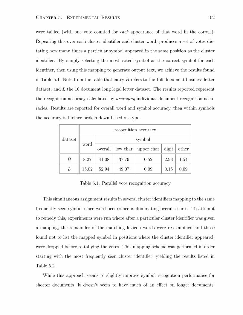
Chapter 5. Experimental Results 102
were tallied (with one vote counted for each appearance of that word in the corpus).
Repeating this over each cluster identifier and cluster word, produces a set of votes dic-
tating how many times a particular symbol appeared in the same position as the cluster
identifier. By simply selecting the most voted symbol as the correct symbol for each
identifier, then using this mapping to generate output text, we achieve the results found
in Table 5.1. Note from the table that entry B refers to the 159 document business letter
dataset, and L the 10 document long legal letter dataset. The results reported represent
the recognition accuracy calculated by averaging individual document recognition accu-
racies. Results are reported for overall word and symbol accuracy, then within symbols
the accuracy is further broken down based on type.
dataset
recognition accuracy
wordsymbol
overall low char upper char digit other
B 8.27 41.08 37.79 0.52 2.93 1.54
L 15.02 52.94 49.07 0.09 0.15 0.09
Table 5.1: Parallel vote recognition accuracy
This simultaneous assignment results in several cluster identifiers mapping to the same
frequently seen symbol since word occurrence is dominating overall scores. To attempt
to remedy this, experiments were run where after a particular cluster identifier was given
a mapping, the remainder of the matching lexicon words were re-examined and those
found not to list the mapped symbol in positions where the cluster identifier appeared,
were dropped before re-tallying the votes. This mapping scheme was performed in order
starting with the most frequently seen cluster identifier, yielding the results listed in
Table 5.2.
While this approach seems to slightly improve symbol recognition performance for
shorter documents, it doesn’t seem to have much of an effect on longer documents.
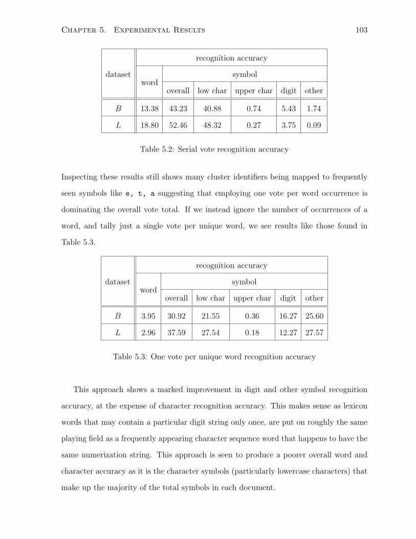
Chapter 5. Experimental Results 103
dataset
recognition accuracy
wordsymbol
overall low char upper char digit other
B 13.38 43.23 40.88 0.74 5.43 1.74
L 18.80 52.46 48.32 0.27 3.75 0.09
Table 5.2: Serial vote recognition accuracy
Inspecting these results still shows many cluster identifiers being mapped to frequently
seen symbols like e, t, a suggesting that employing one vote per word occurrence is
dominating the overall vote total. If we instead ignore the number of occurrences of a
word, and tally just a single vote per unique word, we see results like those found in
Table 5.3.
dataset
recognition accuracy
wordsymbol
overall low char upper char digit other
B 3.95 30.92 21.55 0.36 16.27 25.60
L 2.96 37.59 27.54 0.18 12.27 27.57
Table 5.3: One vote per unique word recognition accuracy
This approach shows a marked improvement in digit and other symbol recognition
accuracy, at the expense of character recognition accuracy. This makes sense as lexicon
words that may contain a particular digit string only once, are put on roughly the same
playing field as a frequently appearing character sequence word that happens to have the
same numerization string. This approach is seen to produce a poorer overall word and
character accuracy as it is the character symbols (particularly lowercase characters) that
make up the majority of the total symbols in each document.

Chapter 5. Experimental Results 104
Improvements can be made first by normalizing the vote count. In this approach,
given a single cluster word and its corresponding list of matching lexicon words, the
proportion of the total time a cluster identifier is seen to map to each symbol in the
list is calculated. A single vote “unit” is then divided into fractional values based on
these proportions. By repeating this over each cluster word, and summing these frac-
tional votes, a normalized estimate can be found. A second improvement can be made
to ensure that uppercase letters and punctuation symbols are appropriately represented.
Since a majority of uppercase letters are seen in the first position of the first word of a
sentence, only those lexicon words in which this is the case are currently added to the
proportional mapping counts for a cluster identifier appearing in the first position. Such
mappings are typically underestimated since there are many more valid first letter capi-
talized words than those that happen to be present in the lexicon. To ensure these counts
for uppercase letters are in reasonable proportions, each matching lowercase lexicon word
has its equivalent word (with the first letter capitalized) added to the lexicon list before
determining proportional votes. A similar strategy is employed for handling punctuation
at the end of a word. Words in the lexicon with an equivalent numerization string, but
which are one character shorter than the current word being mapped are also added
with appropriate punctuation symbols applied when considering proportional counts for
cluster identifiers appearing in the last position of a word. Testing this approach against
the datasets yields the results found in Table 5.4.
dataset
recognition accuracy
wordsymbol
overall low char upper char digit other
B 51.15 68.68 74.38 21.96 8.84 20.42
L 91.39 92.29 97.75 43.66 14.26 32.51
Table 5.4: Normalized vote recognition accuracy
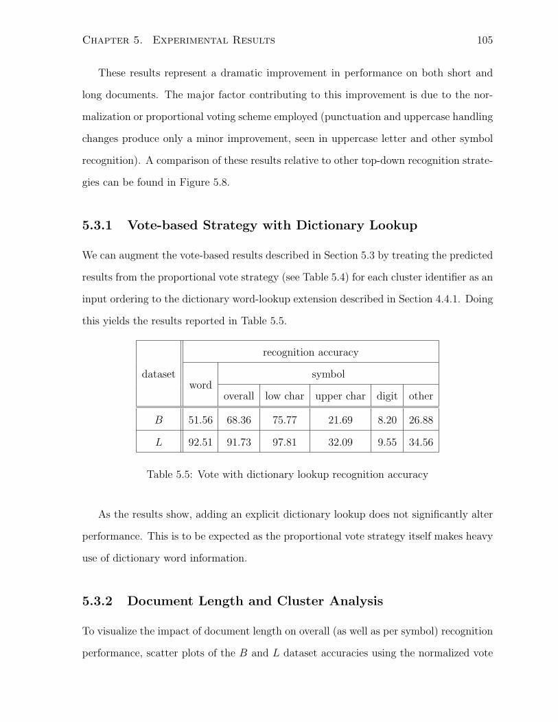
Chapter 5. Experimental Results 105
These results represent a dramatic improvement in performance on both short and
long documents. The major factor contributing to this improvement is due to the nor-
malization or proportional voting scheme employed (punctuation and uppercase handling
changes produce only a minor improvement, seen in uppercase letter and other symbol
recognition). A comparison of these results relative to other top-down recognition strate-
gies can be found in Figure 5.8.
5.3.1 Vote-based Strategy with Dictionary Lookup
We can augment the vote-based results described in Section 5.3 by treating the predicted
results from the proportional vote strategy (see Table 5.4) for each cluster identifier as an
input ordering to the dictionary word-lookup extension described in Section 4.4.1. Doing
this yields the results reported in Table 5.5.
dataset
recognition accuracy
wordsymbol
overall low char upper char digit other
B 51.56 68.36 75.77 21.69 8.20 26.88
L 92.51 91.73 97.81 32.09 9.55 34.56
Table 5.5: Vote with dictionary lookup recognition accuracy
As the results show, adding an explicit dictionary lookup does not significantly alter
performance. This is to be expected as the proportional vote strategy itself makes heavy
use of dictionary word information.
5.3.2 Document Length and Cluster Analysis
To visualize the impact of document length on overall (as well as per symbol) recognition
performance, scatter plots of the B and L dataset accuracies using the normalized vote
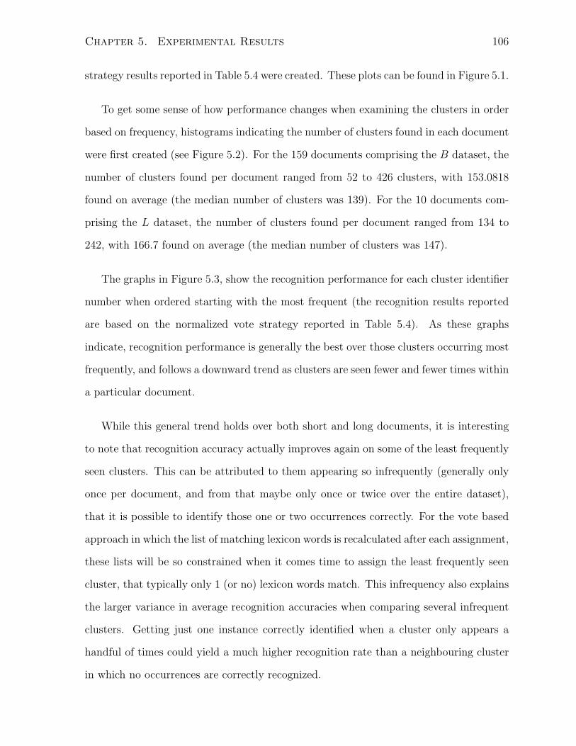
Chapter 5. Experimental Results 106
strategy results reported in Table 5.4 were created. These plots can be found in Figure 5.1.
To get some sense of how performance changes when examining the clusters in order
based on frequency, histograms indicating the number of clusters found in each document
were first created (see Figure 5.2). For the 159 documents comprising the B dataset, the
number of clusters found per document ranged from 52 to 426 clusters, with 153.0818
found on average (the median number of clusters was 139). For the 10 documents com-
prising the L dataset, the number of clusters found per document ranged from 134 to
242, with 166.7 found on average (the median number of clusters was 147).
The graphs in Figure 5.3, show the recognition performance for each cluster identifier
number when ordered starting with the most frequent (the recognition results reported
are based on the normalized vote strategy reported in Table 5.4). As these graphs
indicate, recognition performance is generally the best over those clusters occurring most
frequently, and follows a downward trend as clusters are seen fewer and fewer times within
a particular document.
While this general trend holds over both short and long documents, it is interesting
to note that recognition accuracy actually improves again on some of the least frequently
seen clusters. This can be attributed to them appearing so infrequently (generally only
once per document, and from that maybe only once or twice over the entire dataset),
that it is possible to identify those one or two occurrences correctly. For the vote based
approach in which the list of matching lexicon words is recalculated after each assignment,
these lists will be so constrained when it comes time to assign the least frequently seen
cluster, that typically only 1 (or no) lexicon words match. This infrequency also explains
the larger variance in average recognition accuracies when comparing several infrequent
clusters. Getting just one instance correctly identified when a cluster only appears a
handful of times could yield a much higher recognition rate than a neighbouring cluster
in which no occurrences are correctly recognized.
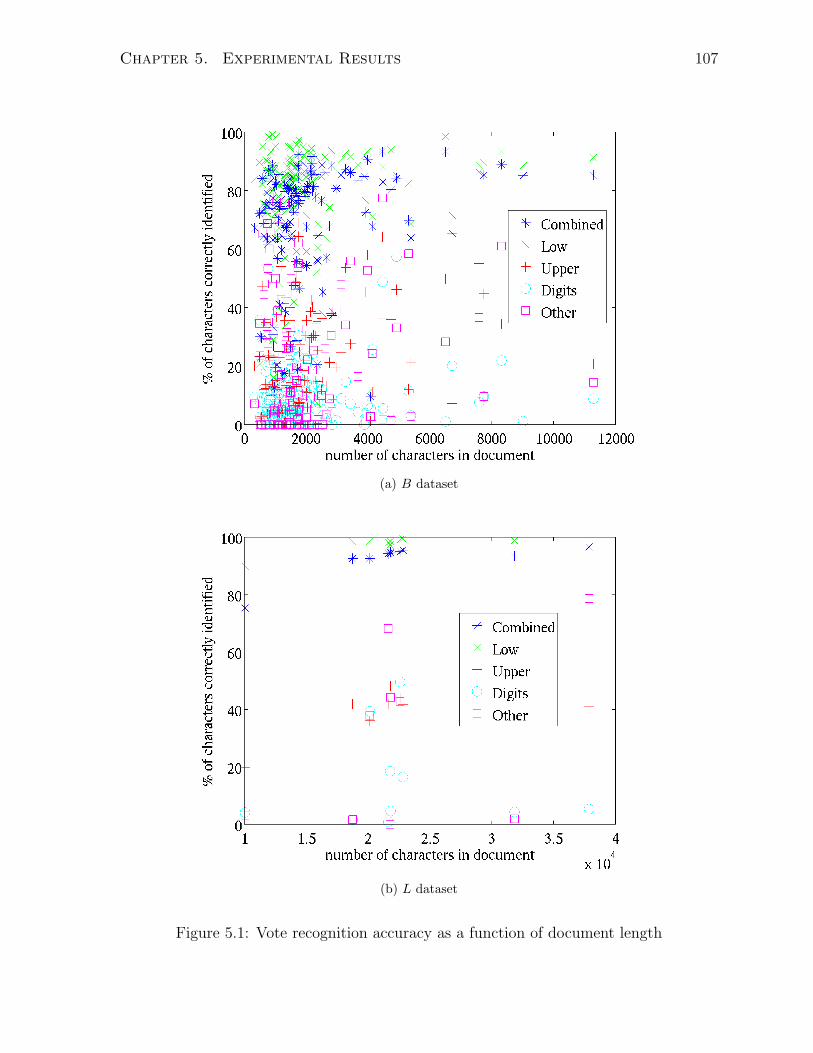
Chapter 5. Experimental Results 107
(a) B dataset
(b) L dataset
Figure 5.1: Vote recognition accuracy as a function of document length
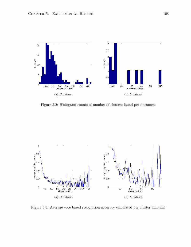
Chapter 5. Experimental Results 108
(a) B dataset (b) L dataset
Figure 5.2: Histogram counts of number of clusters found per document
(a) B dataset (b) L dataset
Figure 5.3: Average vote based recognition accuracy calculated per cluster identifier
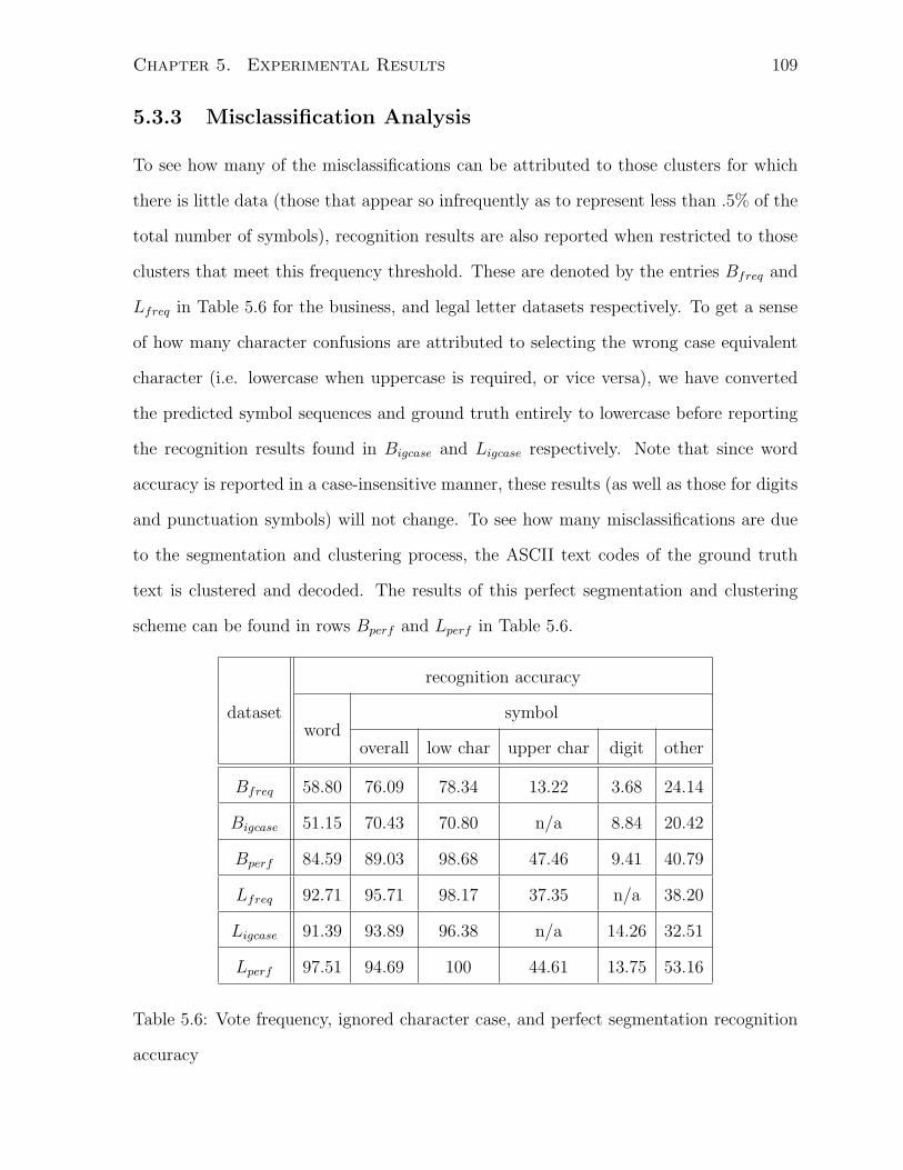
Chapter 5. Experimental Results 109
5.3.3 Misclassification Analysis
To see how many of the misclassifications can be attributed to those clusters for which
there is little data (those that appear so infrequently as to represent less than .5% of the
total number of symbols), recognition results are also reported when restricted to those
clusters that meet this frequency threshold. These are denoted by the entries Bfreq and
Lfreq in Table 5.6 for the business, and legal letter datasets respectively. To get a sense
of how many character confusions are attributed to selecting the wrong case equivalent
character (i.e. lowercase when uppercase is required, or vice versa), we have converted
the predicted symbol sequences and ground truth entirely to lowercase before reporting
the recognition results found in Bigcase and Ligcase respectively. Note that since word
accuracy is reported in a case-insensitive manner, these results (as well as those for digits
and punctuation symbols) will not change. To see how many misclassifications are due
to the segmentation and clustering process, the ASCII text codes of the ground truth
text is clustered and decoded. The results of this perfect segmentation and clustering
scheme can be found in rows Bperf and Lperf in Table 5.6.
dataset
recognition accuracy
wordsymbol
overall low char upper char digit other
Bfreq 58.80 76.09 78.34 13.22 3.68 24.14
Bigcase 51.15 70.43 70.80 n/a 8.84 20.42
Bperf 84.59 89.03 98.68 47.46 9.41 40.79
Lfreq 92.71 95.71 98.17 37.35 n/a 38.20
Ligcase 91.39 93.89 96.38 n/a 14.26 32.51
Lperf 97.51 94.69 100 44.61 13.75 53.16
Table 5.6: Vote frequency, ignored character case, and perfect segmentation recognition
accuracy

Chapter 5. Experimental Results 110
Looking first at the frequency based results, we see that restricting accuracy calcula-
tions to frequently occurring clusters, generally yields slightly improved results. Excep-
tions include digit and upper-case letters, and this is partly caused by the reduction in
the number of such clusters seen in the documents (in fact no digits are seen among the
most frequent clusters in each of the long documents). Misclassifying a single digit or
uppercase letter has a larger impact on reported results since it now represents a larger
portion of the total occurrences of that particular symbol class.
As expected, the overall symbol accuracy improves when ignoring the case of character
symbols during recognition, indicating that at least some of the time the correct character
is predicted, but the wrong case is chosen. The reason why the lowercase accuracy
reported is lower than the results reported in Table 5.4 is because this accuracy now
includes all the former uppercase characters too.
Assuming a perfect segmentation and clustering improves both sets of results signifi-
cantly. In particular, lowercase characters are now recognized with accuracy rates likely
to surpass most shape-based classifiers (though digits, and punctuation would most likely
remain far worse).
5.4 Within-Word Positional Count Strategy
In our positional approach, we first collect positional statistics on words up to 15 char-
acters in length (in both the corpus and the cluster word sequence). The value of 15
was chosen since this was shown to cover over 98% of the unique words seen in a large
collection of varying documents [28]. By occurrence, words of length 15 or less represent
over 99.8% of the total word count. A squared Euclidean distance metric is used to
calculate how similar each cluster identifier’s positional statistics are to each symbol’s
statistics (as estimated from appearances in the corpus). Instead of using the raw count
values at each position (since these could vary drastically if the corpus is much longer
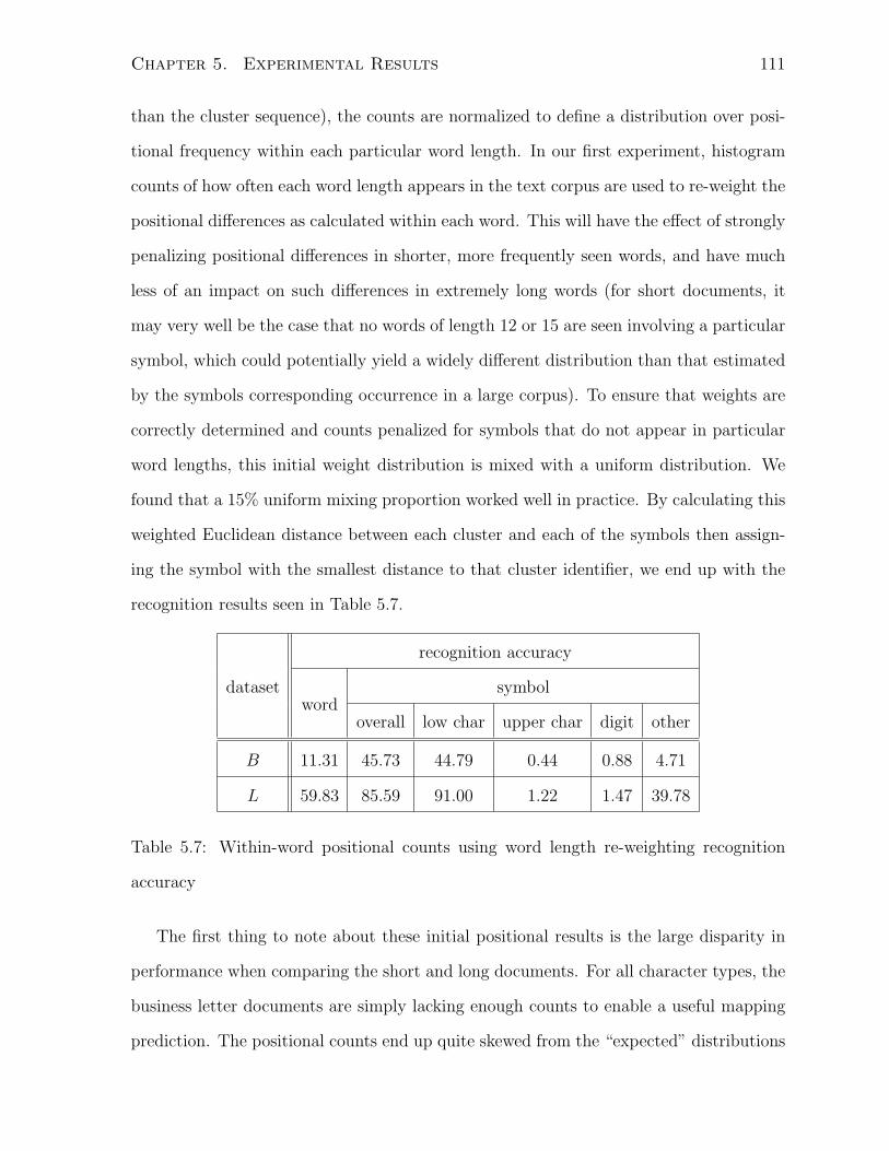
Chapter 5. Experimental Results 111
than the cluster sequence), the counts are normalized to define a distribution over posi-
tional frequency within each particular word length. In our first experiment, histogram
counts of how often each word length appears in the text corpus are used to re-weight the
positional differences as calculated within each word. This will have the effect of strongly
penalizing positional differences in shorter, more frequently seen words, and have much
less of an impact on such differences in extremely long words (for short documents, it
may very well be the case that no words of length 12 or 15 are seen involving a particular
symbol, which could potentially yield a widely different distribution than that estimated
by the symbols corresponding occurrence in a large corpus). To ensure that weights are
correctly determined and counts penalized for symbols that do not appear in particular
word lengths, this initial weight distribution is mixed with a uniform distribution. We
found that a 15% uniform mixing proportion worked well in practice. By calculating this
weighted Euclidean distance between each cluster and each of the symbols then assign-
ing the symbol with the smallest distance to that cluster identifier, we end up with the
recognition results seen in Table 5.7.
dataset
recognition accuracy
wordsymbol
overall low char upper char digit other
B 11.31 45.73 44.79 0.44 0.88 4.71
L 59.83 85.59 91.00 1.22 1.47 39.78
Table 5.7: Within-word positional counts using word length re-weighting recognition
accuracy
The first thing to note about these initial positional results is the large disparity in
performance when comparing the short and long documents. For all character types, the
business letter documents are simply lacking enough counts to enable a useful mapping
prediction. The positional counts end up quite skewed from the “expected” distributions
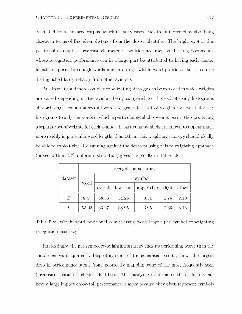
Chapter 5. Experimental Results 112
estimated from the large corpus, which in many cases leads to an incorrect symbol lying
closest in terms of Euclidean distance from the cluster identifier. The bright spot in this
positional attempt is lowercase character recognition accuracy on the long documents,
whose recognition performance can in a large part be attributed to having each cluster
identifier appear in enough words and in enough within-word positions that it can be
distinguished fairly reliably from other symbols.
An alternate and more complex re-weighting strategy can be explored in which weights
are varied depending on the symbol being compared to. Instead of using histograms
of word length counts across all words to generate a set of weights, we can tailor the
histograms to only the words in which a particular symbol is seen to occur, thus producing
a separate set of weights for each symbol. If particular symbols are known to appear much
more readily in particular word lengths than others, this weighting strategy should ideally
be able to exploit this. Re-running against the datasets using this re-weighting approach
(mixed with a 15% uniform distribution) gives the results in Table 5.8
dataset
recognition accuracy
wordsymbol
overall low char upper char digit other
B 8.47 38.33 34.26 0.51 1.76 2.10
L 55.93 83.27 88.95 3.95 2.66 8.18
Table 5.8: Within-word positional counts using word length per symbol re-weighting
recognition accuracy
Interestingly, the per symbol re-weighting strategy ends up performing worse than the
simple per word approach. Inspecting some of the generated results, shows the largest
drop in performance stems from incorrectly mapping some of the most frequently seen
(lowercase character) cluster identifiers. Misclassifying even one of these clusters can
have a large impact on overall performance, simply because they often represent symbols
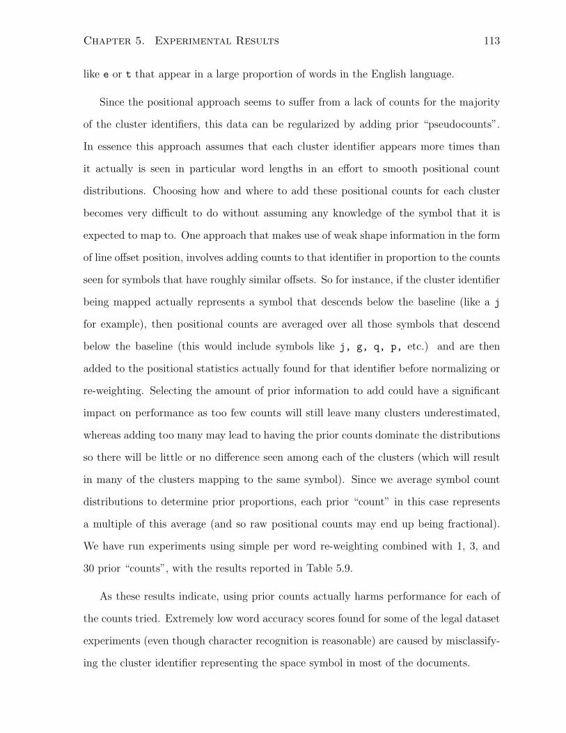
Chapter 5. Experimental Results 113
like e or t that appear in a large proportion of words in the English language.
Since the positional approach seems to suffer from a lack of counts for the majority
of the cluster identifiers, this data can be regularized by adding prior “pseudocounts”.
In essence this approach assumes that each cluster identifier appears more times than
it actually is seen in particular word lengths in an effort to smooth positional count
distributions. Choosing how and where to add these positional counts for each cluster
becomes very difficult to do without assuming any knowledge of the symbol that it is
expected to map to. One approach that makes use of weak shape information in the form
of line offset position, involves adding counts to that identifier in proportion to the counts
seen for symbols that have roughly similar offsets. So for instance, if the cluster identifier
being mapped actually represents a symbol that descends below the baseline (like a j
for example), then positional counts are averaged over all those symbols that descend
below the baseline (this would include symbols like j, g, q, p, etc.) and are then
added to the positional statistics actually found for that identifier before normalizing or
re-weighting. Selecting the amount of prior information to add could have a significant
impact on performance as too few counts will still leave many clusters underestimated,
whereas adding too many may lead to having the prior counts dominate the distributions
so there will be little or no difference seen among each of the clusters (which will result
in many of the clusters mapping to the same symbol). Since we average symbol count
distributions to determine prior proportions, each prior “count” in this case represents
a multiple of this average (and so raw positional counts may end up being fractional).
We have run experiments using simple per word re-weighting combined with 1, 3, and
30 prior “counts”, with the results reported in Table 5.9.
As these results indicate, using prior counts actually harms performance for each of
the counts tried. Extremely low word accuracy scores found for some of the legal dataset
experiments (even though character recognition is reasonable) are caused by misclassify-
ing the cluster identifier representing the space symbol in most of the documents.
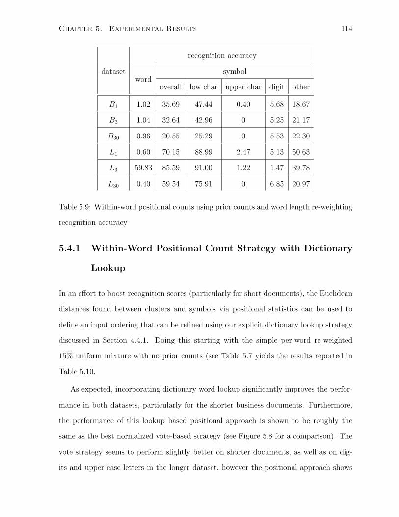
Chapter 5. Experimental Results 114
dataset
recognition accuracy
wordsymbol
overall low char upper char digit other
B1 1.02 35.69 47.44 0.40 5.68 18.67
B3 1.04 32.64 42.96 0 5.25 21.17
B30 0.96 20.55 25.29 0 5.53 22.30
L1 0.60 70.15 88.99 2.47 5.13 50.63
L3 59.83 85.59 91.00 1.22 1.47 39.78
L30 0.40 59.54 75.91 0 6.85 20.97
Table 5.9: Within-word positional counts using prior counts and word length re-weighting
recognition accuracy
5.4.1 Within-Word Positional Count Strategy with Dictionary
Lookup
In an effort to boost recognition scores (particularly for short documents), the Euclidean
distances found between clusters and symbols via positional statistics can be used to
define an input ordering that can be refined using our explicit dictionary lookup strategy
discussed in Section 4.4.1. Doing this starting with the simple per-word re-weighted
15% uniform mixture with no prior counts (see Table 5.7 yields the results reported in
Table 5.10.
As expected, incorporating dictionary word lookup significantly improves the perfor-
mance in both datasets, particularly for the shorter business documents. Furthermore,
the performance of this lookup based positional approach is shown to be roughly the
same as the best normalized vote-based strategy (see Figure 5.8 for a comparison). The
vote strategy seems to perform slightly better on shorter documents, as well as on dig-
its and upper case letters in the longer dataset, however the positional approach shows
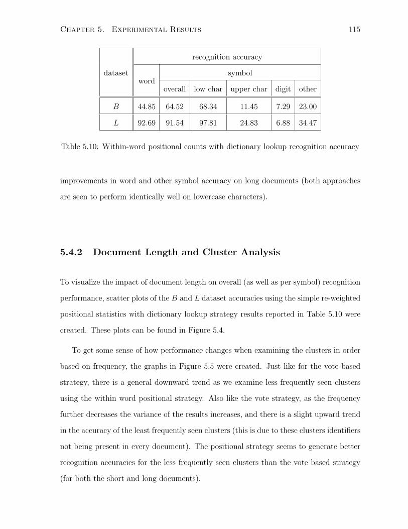
Chapter 5. Experimental Results 115
dataset
recognition accuracy
wordsymbol
overall low char upper char digit other
B 44.85 64.52 68.34 11.45 7.29 23.00
L 92.69 91.54 97.81 24.83 6.88 34.47
Table 5.10: Within-word positional counts with dictionary lookup recognition accuracy
improvements in word and other symbol accuracy on long documents (both approaches
are seen to perform identically well on lowercase characters).
5.4.2 Document Length and Cluster Analysis
To visualize the impact of document length on overall (as well as per symbol) recognition
performance, scatter plots of the B and L dataset accuracies using the simple re-weighted
positional statistics with dictionary lookup strategy results reported in Table 5.10 were
created. These plots can be found in Figure 5.4.
To get some sense of how performance changes when examining the clusters in order
based on frequency, the graphs in Figure 5.5 were created. Just like for the vote based
strategy, there is a general downward trend as we examine less frequently seen clusters
using the within word positional strategy. Also like the vote strategy, as the frequency
further decreases the variance of the results increases, and there is a slight upward trend
in the accuracy of the least frequently seen clusters (this is due to these clusters identifiers
not being present in every document). The positional strategy seems to generate better
recognition accuracies for the less frequently seen clusters than the vote based strategy
(for both the short and long documents).

Chapter 5. Experimental Results 116
(a) B dataset
(b) L dataset
Figure 5.4: Positional count recognition accuracy as a function of document length

Chapter 5. Experimental Results 117
(a) B dataset (b) L dataset
Figure 5.5: Average positional count based recognition accuracy calculated per cluster
identifier
5.4.3 Misclassification Analysis
To get some handle on where misclassifications are made using the positional statistics
approach, a perfect cluster segmentation is simulated, as are the original cluster results
when recognition performance is calculated only on those symbols that make up at least
.5% of the total elements found in the document, and the results calculated when char-
acter case is ignored. These experimental results can be found in Table 5.11.
Examining the frequency based results shows a marked drop in performance over
accuracies calculated using the entire dataset. For uppercase characters and digits, these
symbols only appear in the most frequent documents in a handful of documents, and in
almost every case they were incorrectly recognized a majority of the time.
Ignoring character case shows small improvements in overall character accuracy in
both short and long documents, indicating that at least some of the time, the correct
character is identified, but its case is incorrect.
Like the vote-based strategy, a perfect segmentation drastically improves performance
over each symbol type for the positional statistic strategy. Lowercase character recogni-
tion is perfect over each of the long documents, and on-par with shape-based classifiers
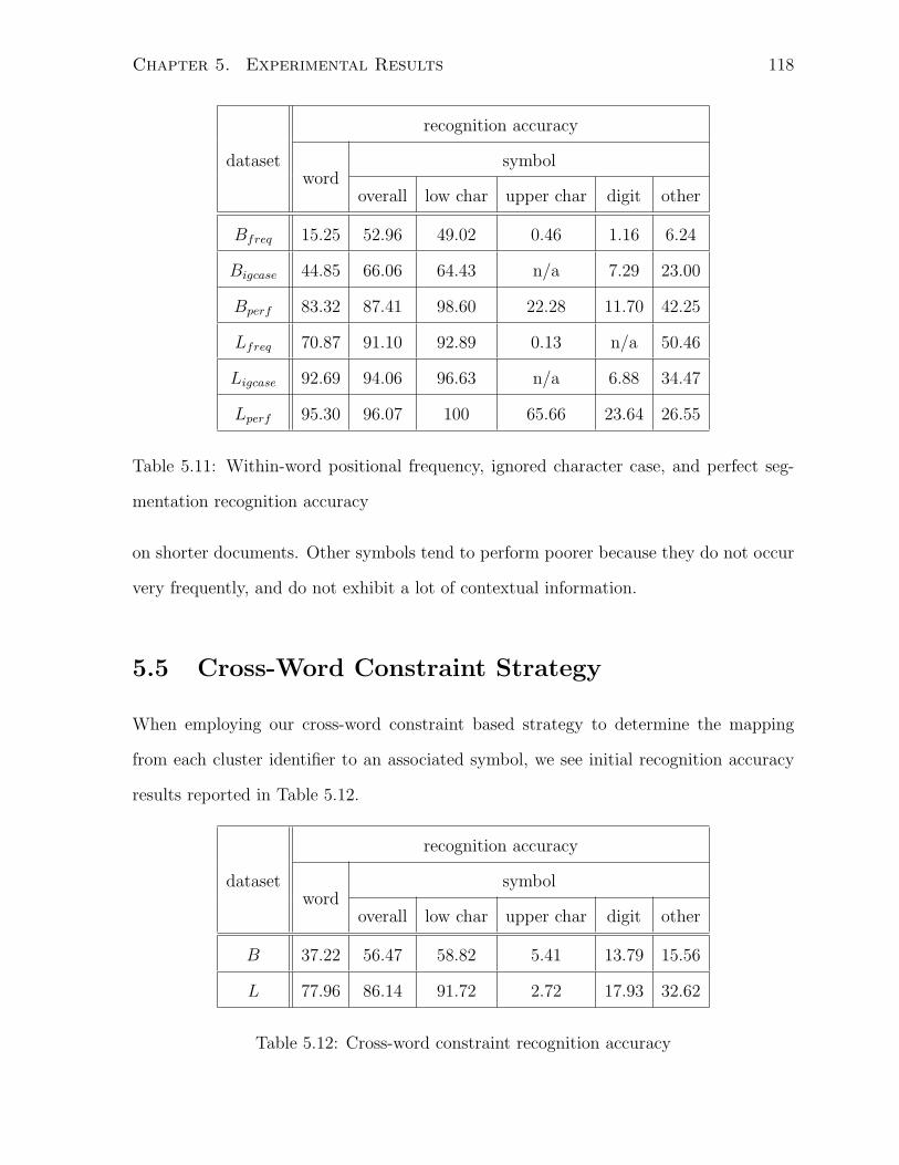
Chapter 5. Experimental Results 118
dataset
recognition accuracy
wordsymbol
overall low char upper char digit other
Bfreq 15.25 52.96 49.02 0.46 1.16 6.24
Bigcase 44.85 66.06 64.43 n/a 7.29 23.00
Bperf 83.32 87.41 98.60 22.28 11.70 42.25
Lfreq 70.87 91.10 92.89 0.13 n/a 50.46
Ligcase 92.69 94.06 96.63 n/a 6.88 34.47
Lperf 95.30 96.07 100 65.66 23.64 26.55
Table 5.11: Within-word positional frequency, ignored character case, and perfect seg-
mentation recognition accuracy
on shorter documents. Other symbols tend to perform poorer because they do not occur
very frequently, and do not exhibit a lot of contextual information.
5.5 Cross-Word Constraint Strategy
When employing our cross-word constraint based strategy to determine the mapping
from each cluster identifier to an associated symbol, we see initial recognition accuracy
results reported in Table 5.12.
dataset
recognition accuracy
wordsymbol
overall low char upper char digit other
B 37.22 56.47 58.82 5.41 13.79 15.56
L 77.96 86.14 91.72 2.72 17.93 32.62
Table 5.12: Cross-word constraint recognition accuracy
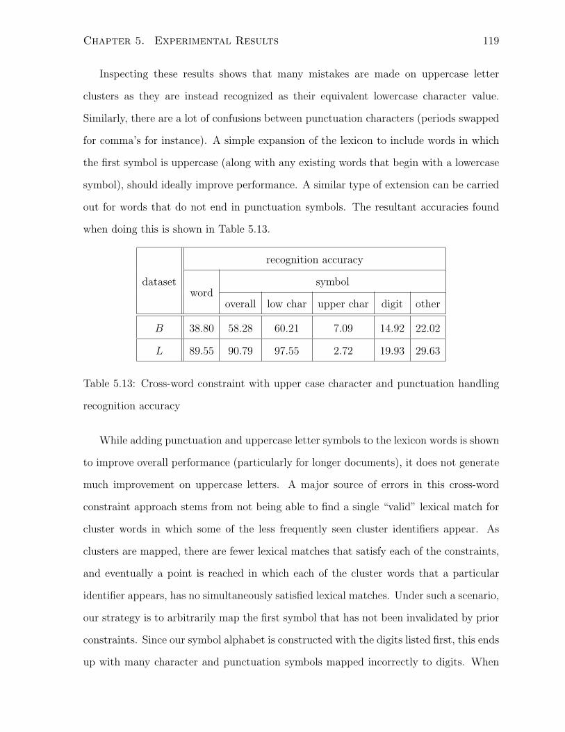
Chapter 5. Experimental Results 119
Inspecting these results shows that many mistakes are made on uppercase letter
clusters as they are instead recognized as their equivalent lowercase character value.
Similarly, there are a lot of confusions between punctuation characters (periods swapped
for comma’s for instance). A simple expansion of the lexicon to include words in which
the first symbol is uppercase (along with any existing words that begin with a lowercase
symbol), should ideally improve performance. A similar type of extension can be carried
out for words that do not end in punctuation symbols. The resultant accuracies found
when doing this is shown in Table 5.13.
dataset
recognition accuracy
wordsymbol
overall low char upper char digit other
B 38.80 58.28 60.21 7.09 14.92 22.02
L 89.55 90.79 97.55 2.72 19.93 29.63
Table 5.13: Cross-word constraint with upper case character and punctuation handling
recognition accuracy
While adding punctuation and uppercase letter symbols to the lexicon words is shown
to improve overall performance (particularly for longer documents), it does not generate
much improvement on uppercase letters. A major source of errors in this cross-word
constraint approach stems from not being able to find a single “valid” lexical match for
cluster words in which some of the less frequently seen cluster identifiers appear. As
clusters are mapped, there are fewer lexical matches that satisfy each of the constraints,
and eventually a point is reached in which each of the cluster words that a particular
identifier appears, has no simultaneously satisfied lexical matches. Under such a scenario,
our strategy is to arbitrarily map the first symbol that has not been invalidated by prior
constraints. Since our symbol alphabet is constructed with the digits listed first, this ends
up with many character and punctuation symbols mapped incorrectly to digits. When
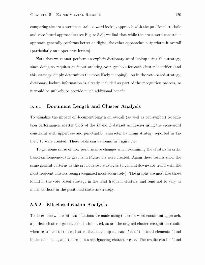
Chapter 5. Experimental Results 120
comparing the cross-word constrained word lookup approach with the positional statistic
and vote-based approaches (see Figure 5.8), we find that while the cross-word constraint
approach generally performs better on digits, the other approaches outperform it overall
(particularly on upper case letters).
Note that we cannot perform an explicit dictionary word lookup using this strategy,
since doing so requires an input ordering over symbols for each cluster identifier (and
this strategy simply determines the most likely mapping). As in the vote-based strategy,
dictionary lookup information is already included as part of the recognition process, so
it would be unlikely to provide much additional benefit.
5.5.1 Document Length and Cluster Analysis
To visualize the impact of document length on overall (as well as per symbol) recogni-
tion performance, scatter plots of the B and L dataset accuracies using the cross-word
constraint with uppercase and punctuation character handling strategy reported in Ta-
ble 5.13 were created. These plots can be found in Figure 5.6.
To get some sense of how performance changes when examining the clusters in order
based on frequency, the graphs in Figure 5.7 were created. Again these results show the
same general patterns as the previous two strategies (a general downward trend with the
most frequent clusters being recognized most accurately). The graphs are most like those
found in the vote based strategy in the least frequent clusters, and tend not to vary as
much as those in the positional statistic strategy.
5.5.2 Misclassification Analysis
To determine where misclassifications are made using the cross-word constraint approach,
a perfect cluster segmentation is simulated, as are the original cluster recognition results
when restricted to those clusters that make up at least .5% of the total elements found
in the document, and the results when ignoring character case. The results can be found
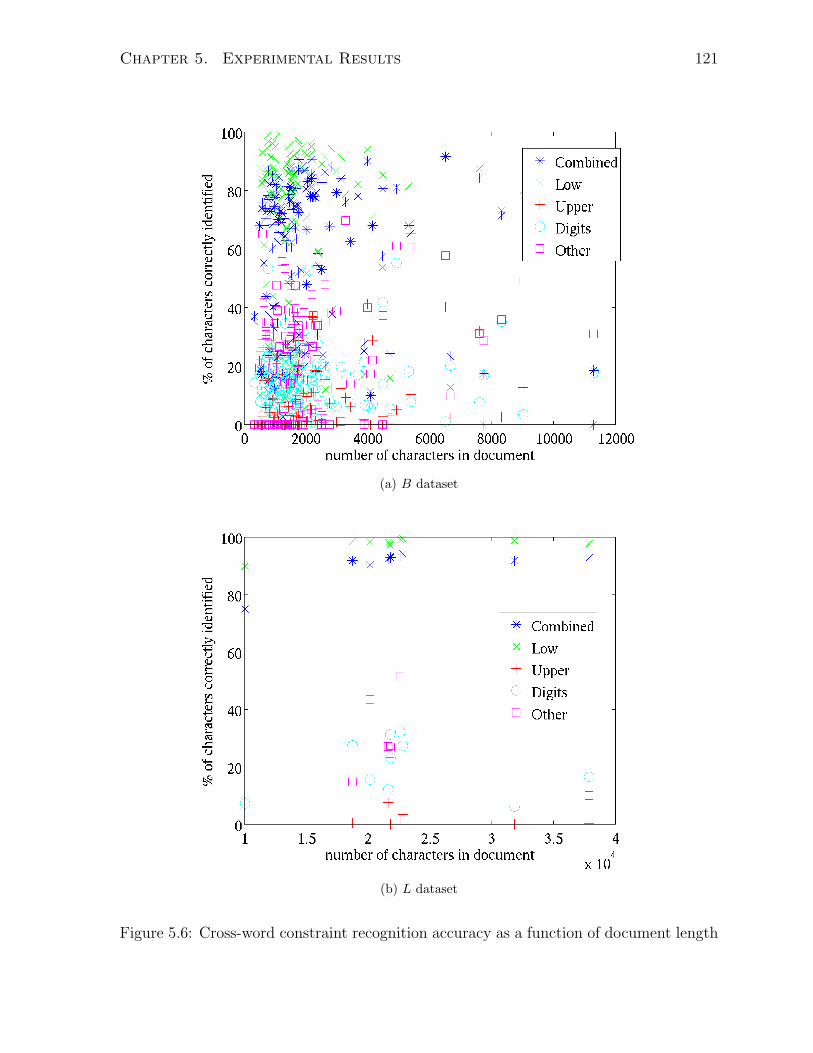
Chapter 5. Experimental Results 121
(a) B dataset
(b) L dataset
Figure 5.6: Cross-word constraint recognition accuracy as a function of document length
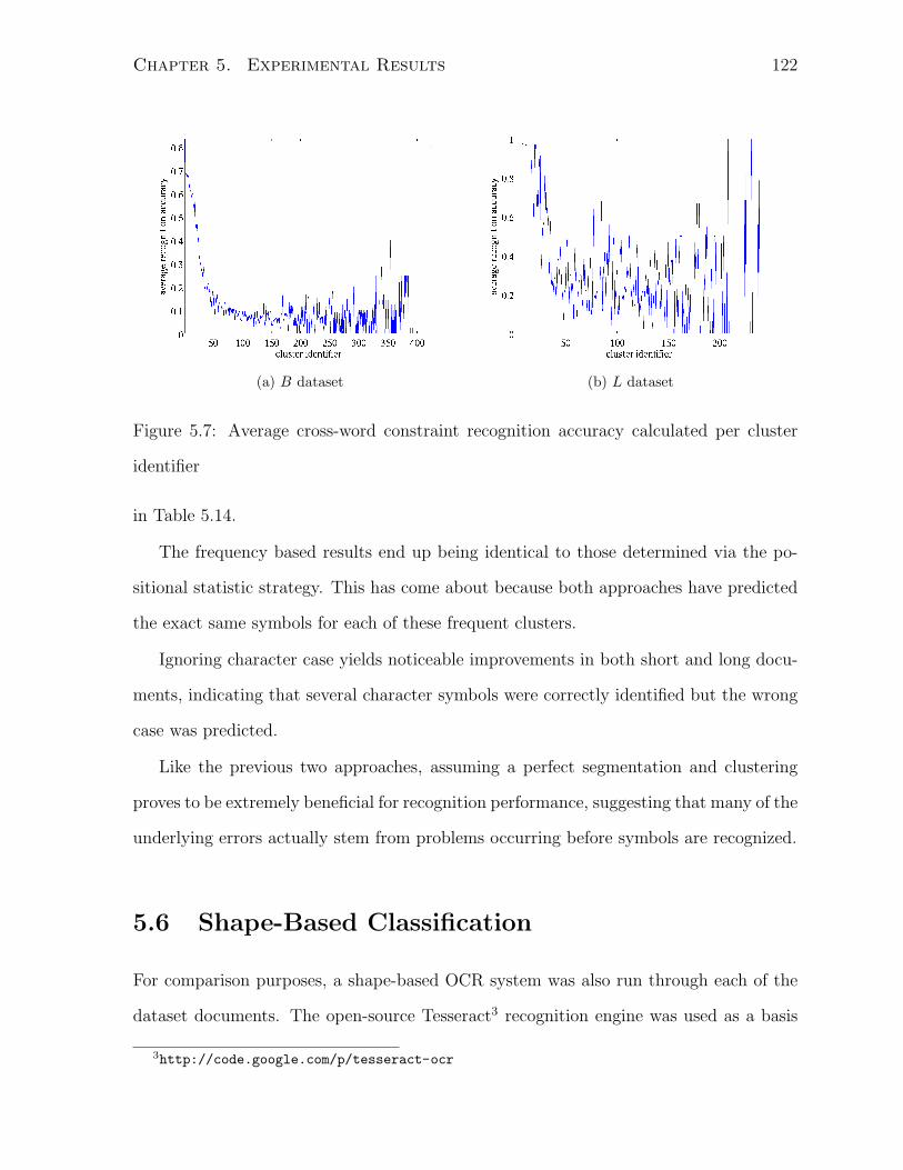
Chapter 5. Experimental Results 122
(a) B dataset (b) L dataset
Figure 5.7: Average cross-word constraint recognition accuracy calculated per cluster
identifier
in Table 5.14.
The frequency based results end up being identical to those determined via the po-
sitional statistic strategy. This has come about because both approaches have predicted
the exact same symbols for each of these frequent clusters.
Ignoring character case yields noticeable improvements in both short and long docu-
ments, indicating that several character symbols were correctly identified but the wrong
case was predicted.
Like the previous two approaches, assuming a perfect segmentation and clustering
proves to be extremely beneficial for recognition performance, suggesting that many of the
underlying errors actually stem from problems occurring before symbols are recognized.
5.6 Shape-Based Classification
For comparison purposes, a shape-based OCR system was also run through each of the
dataset documents. The open-source Tesseract3 recognition engine was used as a basis
3http://code.google.com/p/tesseract-ocr
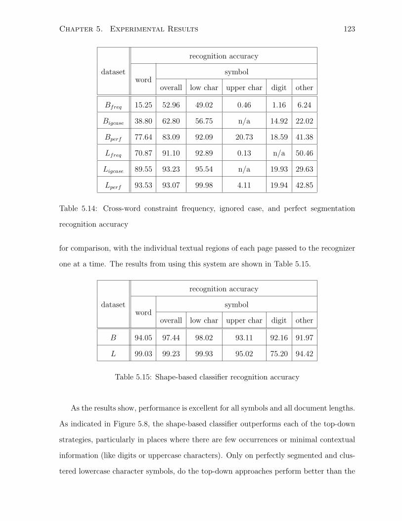
Chapter 5. Experimental Results 123
dataset
recognition accuracy
wordsymbol
overall low char upper char digit other
Bfreq 15.25 52.96 49.02 0.46 1.16 6.24
Bigcase 38.80 62.80 56.75 n/a 14.92 22.02
Bperf 77.64 83.09 92.09 20.73 18.59 41.38
Lfreq 70.87 91.10 92.89 0.13 n/a 50.46
Ligcase 89.55 93.23 95.54 n/a 19.93 29.63
Lperf 93.53 93.07 99.98 4.11 19.94 42.85
Table 5.14: Cross-word constraint frequency, ignored case, and perfect segmentation
recognition accuracy
for comparison, with the individual textual regions of each page passed to the recognizer
one at a time. The results from using this system are shown in Table 5.15.
dataset
recognition accuracy
wordsymbol
overall low char upper char digit other
B 94.05 97.44 98.02 93.11 92.16 91.97
L 99.03 99.23 99.93 95.02 75.20 94.42
Table 5.15: Shape-based classifier recognition accuracy
As the results show, performance is excellent for all symbols and all document lengths.
As indicated in Figure 5.8, the shape-based classifier outperforms each of the top-down
strategies, particularly in places where there are few occurrences or minimal contextual
information (like digits or uppercase characters). Only on perfectly segmented and clus-
tered lowercase character symbols, do the top-down approaches perform better than the

Chapter 5. Experimental Results 124
shape-based approach. It should also be noted that most if not all of the documents
in these datasets are set in standard font faces and sizes, which means that Tesseract’s
symbol classifier will most likely have seen these fonts as part of a prior training process.
5.7 Atypical Font Results
While shape-based classifiers have been shown to outperform the top-down strategies
for the most part on the UNLV B and L datasets, it is worth exploring performance on
datasets written in fonts in which a shape-based classifier has not previously been trained.
To test this, we ran each of our top-down classifiers through the synthetically generated
italicized Reuters document discussed in Chapter 1, a sample page of this dataset can
be seen in Figure 1.4. This document contains 19,635 symbols spread over eight pages.
The results of running each of our approaches (using the best found normalizations and
other settings) is shown in Table 5.16.
dataset
recognition accuracy
wordsymbol
overall low char upper char digit other
Reutvote 92.33 94.64 97.86 93.17 84.28 100
Reutpos 92.54 94.67 97.87 92.46 84.28 100
Reutconst 92.11 92.99 98.21 92.10 41.02 100
Table 5.16: Top-down synthetic document recognition accuracy
When compared with the results in Table 1.2 we see that for lowercase letters, each
of our top-down approaches outperforms all but one of the commercial systems (see
Figure 5.10a). Our approaches also outperform all of these systems on punctuation and
other symbols. For uppercase letter, and especially digit performance, it seems that
the shape-based classifiers still perform better. As can be seen from Figure 5.9, several
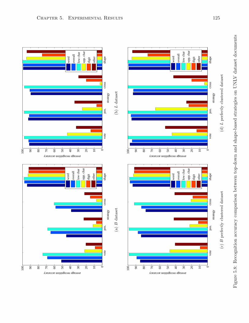
Chapter 5. Experimental Results 125
vote
po
s.
cros
ssh
ape
0102030405060708090100
stra
tegy
average recognition accuracy
wor
d
over
all
low
cha
r
upp.
cha
r
digi
t
othe
r
(a)
Bda
tase
t
vote
po
s.
cros
ssh
ape
0102030405060708090100
stra
tegy
average recognition accuracy
wor
d
over
all
low
cha
r
upp.
cha
r
digi
t
othe
r
(b)
Lda
tase
t
vote
po
s.
cros
ssh
ape
0102030405060708090100
stra
tegy
average recognition accuracy
wor
d
over
all
low
cha
r
upp.
cha
r
digi
t
othe
r
(c)
Bpe
rfec
tly
clus
tere
dda
tase
t
vote
po
s.
cros
ssh
ape
0102030405060708090100
stra
tegy
average recognition accuracy
wor
d
over
all
low
cha
r
upp.
cha
r
digi
t
othe
r
(d)
Lpe
rfec
tly
clus
tere
dda
tase
t
Fig
ure
5.8:
Rec
ognit
ion
accu
racy
com
par
ison
bet
wee
nto
p-d
own
and
shap
e-bas
edst
rate
gies
onU
NLV
dat
aset
docu
men
ts

Chapter 5. Experimental Results 126
cluster centroids were not split apart during the clustering process, resulting in many of
the recognition errors seen. If we assume a perfect clustering we obtain the results shown
in Table 5.17.
Figure 5.9: Synthetic document cluster averages
dataset
recognition accuracy
wordsymbol
overall low char upper char digit other
Reutvote 99.79 99.97 100 99.04 100 100
Reutpos 99.79 99.96 100 98.80 100 100
Reutconst 99.79 97.75 100 98.80 49.02 100
Table 5.17: Top-down perfectly clustered synthetic document recognition accuracy
As this table and Figure 5.10b show, each of the top-down approaches performs
extremely well, outperforming each of the shape-based approaches on each symbol type
(with the exception of the cross-word constraint approach applied to digits). Lowercase

Chapter 5. Experimental Results 127
letter, and punctuation symbol recognition is perfect, something which none of the shape-
based classifiers was shown to achieve.
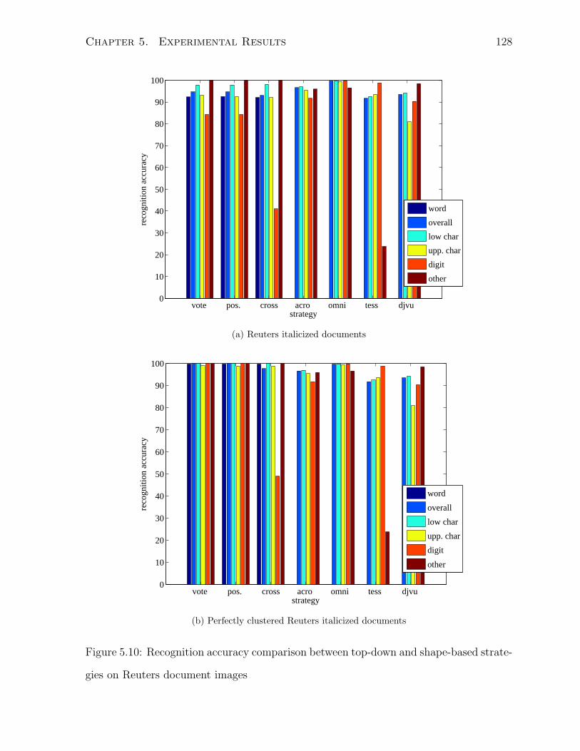
Chapter 5. Experimental Results 128
vote pos. cross acro omni tess djvu 0
10
20
30
40
50
60
70
80
90
100
strategy
reco
gniti
on a
ccur
acy
word
overall
low char
upp. char
digit
other
(a) Reuters italicized documents
vote pos. cross acro omni tess djvu 0
10
20
30
40
50
60
70
80
90
100
strategy
reco
gniti
on a
ccur
acy
word
overall
low char
upp. char
digit
other
(b) Perfectly clustered Reuters italicized documents
Figure 5.10: Recognition accuracy comparison between top-down and shape-based strate-
gies on Reuters document images
Chapter 6
Conclusions
The work in this thesis has explored an alternate approach to symbol recognition that
is currently under-represented in OCR system research and development. As the ex-
perimental results presented in Chapter 5 show, our top-down decoding strategies can
perform roughly equivalent to shape based classifiers when presented with enough well
segmented input data.
6.1 Benefits of our Approach
Performing character recognition using purely contextual cues, after clustering similar
shaped-symbols together offers several advantages and benefits over the traditional shape-
based classifier approach. First and foremost, our approach is font independent, and able
to adapt or generalize to any consistently presented fonts given as input (regardless of
how unique they may be). Assuming the same level of noise and content, the symbols
of documents written uniformly in arbitrarily different font faces will be recognized with
exactly the same accuracy, something that will not hold for shape-based classifiers if at
least one of the fonts was not part of the original training set.
Another advantage of a top-down recognition strategy involves the ease with which
such a system can be re-targeted to work with documents written in other phonetic
129
Chapter 6. Conclusions 130
languages. By simply switching the corpus and symbol alphabet with those of the new
language to be recognized, the rest of the process remains unchanged. Such an approach
can even be extended to niche applications like the recognition of bank cheques, sheet
music, or chess moves in which the list of symbols seen and “language” lexicon are suitably
constrained (assuming that these atomic symbols can be segmented and appear as part
of a hierarchical “word-like” structure).
Finally, our top-down approach is able to exploit modern symbolic compression
schemes like JBIG2 [24], and perform recognition on these compressed document im-
ages directly. Symbolic compression schemes are designed to operate on binary images,
and take advantage of repeatedly seen sub-image patterns (which are bountiful in textual
documents). JBIG2 is an industry standard compression scheme that is used by several
popular image formats including Adobe’s PDF format (DjVu actually uses a slightly dif-
ferent symbolic compression scheme known as JB2). These schemes work by calculating
the connected components in an uncompressed document image, then they attempt to
find similar shaped components elsewhere in the image (much like our clustering pro-
cedure described in Chapter 3). For lossless compression schemes, a single template
sub-image is stored, and everywhere else that a roughly similar shape appears, its off-
set co-ordinates in the document are stored. Finally, the residual or difference between
the template and the similar shaped occurrence is stored. In contrast, lossy versions of
this compression scheme simply throw away these residuals during compression (but are
otherwise identical to lossless schemes). Not only can our recognition approach work
directly with these compressed inputs and offset locations, they actually work faster on
these documents than on their uncompressed equivalents. The reason for this is that the
clustering stage of our approach represents a significant portion of the overall processing
time required. Starting from a set of templates and their corresponding offsets, this initial
clustering can be used as a starting point for the top-down recognition process, though
a split or merge refinement is often necessary to ensure that components correspond to
Chapter 6. Conclusions 131
individual symbol images.
6.2 Future Work
As our work was largely exploratory in nature, there remain several areas for further
pursuit. We have chosen to binarize colour or grayscale documents prior to further
processing, largely for computational efficiency reasons. In doing so we lose useful in-
formation initially present in the document that could potentially harm clustering and
subsequent recognition performance. As an example, consider a synthetic font which
happens to be designed so that the glyphs are composed of pixel intensity gradients that
shift from dark to light (as some logotypes do, to indicate motion). Under our current
approach, these gradient intensities are simply chopped at a fixed point, which could
yield a partial symbol. If this is done consistently over the entire document this is less
of a problem, but if done for only some occurrences of a particular symbol, grouping all
occurrences under the same cluster becomes difficult (other problems arise when looking
for potential split points if such a component is actually composed of multiple symbols).
As the experimental results in Chapter 5 indicate, a significant portion of misclassifi-
cation errors are originally caused by errors in the clustering process, in particular many
fused symbols remain even after split refinement procedures. This biases the positional
statistics and yields invalid numerization strings which ultimately ends in incorrect or
non-existent corpus dictionary words to determine the mappings from. When mappings
are assigned one-by-one, the first incorrect mapping can skew or incorrectly constrain
further word lookup, and thus subsequent recognition assignments (i.e. after the first
mistake, the problem snowballs). As alluded to in Chapter 4, an improvement would be
to use the information found from an initial recognition of the cluster identifiers, to go
back and look for clusters that should be re-segmented.
Another simple correction that ideally should be implemented involves handling words
Chapter 6. Conclusions 132
that are hyphenated and split over multiple lines. Some sort of pre-processing should be
carried out prior to recognition to try and identify sub-words that have been hyphenated
and split. Hyphen symbols are fairly consistent in terms of baseline and x-height offset,
aspect ratio and density so identifying them in a font-free manner should be possible.
Looking for components with no right neighbouring component (within a reasonable
distance) that are much wider than they are taller, and whose bottom bounding box
co-ordinate lies above the baseline should allow one to identify the hyphens, which can
then be used to glue together the adjacent word halve on the next line prior to cluster
word statistic gathering and contextual recognition.
More detailed statistical models could also be employed to improve the recognition
results, particularly for infrequently seen clusters. For long documents, most of the
lowercase character symbols can be recognized quite accurately, however for a lot of
individuals, scanning is typically done on short one or two page documents. Even for
longer documents, symbols that are seldom seen, or those for which there is almost no
contextual information will require alternate strategies to be recognized correctly. As an
example, if given an input string of the form 45x69, where x remains the only unknown
mapped symbol, even if it was guaranteed that x was a digit, the probability of which
particular digit x represented is essentially uniform. While 0,1,9 may be slightly more
common in large corpora (because of things like prices, and the human tendency of
rounding discussed digit strings to whole numbers), context alone can not distinguish
the correct digit for x.
Our implementation also currently relies on setting several threshold parameters by
hand, prior to segmenting, clustering, and recognizing document images. Ideally, these
parameters should be tuned or learned automatically, using information found in earlier
stages of the process. For instance, during the clustering phase, the mean or modal aspect
ratio of the connected components can be combined with variance, density, or other pixel
measures to determine suitable cluster matching distance thresholds.
Bibliography
[1] Adnan Amin and Sue Wu. Robust skew detection in mixed text/graphics docu-
ments. In Proceedings of the 8th International Conference on Document Analysis
and Recognition, pages 247–251, 2005.
[2] Henry S. Baird. The skew angle of printed documents. In Lawrence O’Gorman
and R. Kasturi, editors, Document Image Analysis, pages 204–208. IEEE Computer
Society Press, 1995.
[3] Leonard E. Baum, Ted Petrie, George Soules, and Weiss Norman. A maximization
technique occuring in the statistical analysis of probabilistic functions of Markov
chains. The Annals of Mathematical Statistics, 41(1):164–171, February 1970.
[4] Dan S. Bloomberg, Gary E. Kopec, and Lakshmi Dasari. Measuring document
image skew and orientation. In Proceedings of the SPIE Conference on Document
Recognition II, pages 302–316, 1995.
[5] Mindy Bosker. Omnidocument technologies. Proceedings of the IEEE, 80(7):1066–
1078, July 1992.
[6] Richard G. Casey. Text OCR by solving a cryptogram. In Proceedings of the 8th
International Conference on Pattern Recognition, volume 1, pages 349–351, August
1986.
133
Bibliography 134
[7] Richard G. Casey and Eric Lecolinet. A survey of methods and strategies in character
segmentation. IEEE Transactions on Pattern Analysis and Machine Intelligence,
18(7):690–706, July 1996.
[8] R. Cattoni, T. Coianiz, S. Messelodi, and M. Modena. Geometric layout analysis
techniques for document image understanding: a review. Technical report, ITC-
IRST, Via Sommarive, 1998.
[9] F. Cesarini, M. Gori, S. Marinai, and G. Soda. Structured document segmentation
and representation by the modified XY-tree. In Proceedings of the 7th International
Conference on Document Analysis and Recognition, pages 563–566, 2003.
[10] Arthur P. Dempster, Nan Laird, and Donald Rubin. Maximum likelihood from
incomplete data via the EM algorithm. Journal of the Royal Statistical Society.
Series B (Methodological), 39(1):1–38, 1977.
[11] David Doermann, Jian Liang, and Huiping Li. Progress in camera-based document
image analysis. In Proceedings of the 7th International Conference on Document
Analysis and Recognition (ICDAR’03), volume 1, pages 606–616, 2003.
[12] Richard O. Duda and Peter E. Hart. Use of the Hough transformation to detect
lines and curves in pictures. Communications of the ACM, 15(1):11–15, 1972.
[13] D. G. Elliman and I. T. Lancaster. A review of segmentation and contextual analysis
techniques for text recognition. Pattern Recognition, 23(3-4):337–346, 1990.
[14] David W. Embley, Matthew Hurst, Daniel Lopresti, and George Nagy. Table pro-
cessing paradigms: A research survey. International Journal on Document Analysis
and Recognition, 8(2):66–86, May 2006.
[15] David G. Jr. Forney. The Viterbi algorithm. In Proceedings of the IEEE, volume 61,
pages 268–278, March 1973.
Bibliography 135
[16] Hiromichi Fujisawa, Yasuaki Nakano, and Kiyomichi Kurino. Segmentation meth-
ods for character recogntion: From segmentation to document structure analysis.
Proceedings of the IEEE, 80(7):1079–1092, July 1992.
[17] Paul W. Handel. Statistical machine. U.S. Patent 1915993,
http://www.google.com/patents?vid=USPAT1915993, June 1933.
[18] Robert M. Haralick, S. R. Sternberg, and X. Zhuang. Image analysis using mathe-
matical morphology. IEEE Transactions on Pattern Analysis and Machine Intelli-
gence, 9(4):532–550, 1987.
[19] Akihide Hashizume, Pen-Shu Yeh, and Azriel Rosenfeld. A method of detecting
the orientation of aligned components. Pattern Recogntion Letters, 4:125–132, April
1986.
[20] R. B. Hennis. The IBM 1975 optical page reader: System design. IBM Journal of
Research and Development, 12(5):346–353, September 1968.
[21] Tin Kam Ho and George Nagy. OCR with no shape training. In Proceedings of the
15th International Conference on Pattern Recognition (ICPR ’00), volume 4, pages
27–30, 2000.
[22] Tin Kam Ho and George Nagy. Exploration of contextual constraints for character
pre-classification. In Proceedings of the 6th International Conference on Document
Analysis and Recognition (ICDAR ’01), pages 450–454, 2001.
[23] Judith Hochberg, Ppatrick Kelly, Timothy Thomas, and Lila Kerns. Automatic
script identification from document images using cluster-based templates. IEEE
Transactions on Pattern Analysis and Machine Intelligence, 19(2):176–181, 1997.
Bibliography 136
[24] Paul G. Howard, Faouzi Kossentini, Bo Martins, Soren Forchhammer, and William J.
Rucklidge. The emerging JBIG2 standard. IEEE Transactions on Circuits and
Systems for Video Technology, 8(7):838–848, November 1998.
[25] Gary Huang, Andrew McCallum, and Erik Learned-Miller. Cryptogram decoding for
optical character recognition. Technical Report 06-45, University of Massachusetts
Amherst, June 2006.
[26] Simon Kahan, Theo Pavlidis, and Henry S. Baird. On the recognition of printed
characters of any font and size. IEEE Transactions on Pattern Analysis and Machine
Intelligence, 9(2):274–287, March 1987.
[27] Koichi Kise, Akinori Sato, and Motoi Iwata. Segmentation of page images using the
area voronoi diagram. Computer Vision and Image Understanding, 70(3):370–382,
1998.
[28] Henry Kucera and W. Nelson Francis. Computational Analysis of Present-Day
American English. Brown University Press, 1967.
[29] Kevin Laven. Application of statistical pattern recognition to document segmenta-
tion and labelling. Master’s thesis, University of Toronto, 2005.
[30] Kevin Laven, Scott Leishman, and Sam Roweis. A statistical learning approach to
document image analysis. In Proceedings of the 8th International Conference on
Document Analysis and Recognition, volume 1, pages 357–361, 2005.
[31] Yann LeCun, Leon Bossou, Yoshua Bengio, and Patrick Haffner. Gradient-based
learning applied to document recognition. Proceedings of the IEEE, 86(11):2278–
2324, November 1998.
Bibliography 137
[32] Dar-Shyang Lee. Substitution deciphering based on HMMs with application to com-
pressed document processing. IEEE Transactions on Pattern Analysis and Machine
Intelligence, 24(12):1661–1666, December 2002.
[33] Vladimir I. Levenshtein. Binary codes capable of correcting deletions, insertions,
and reversals. Soviet Physics Doklady, 10:707–710, February 1966.
[34] David D. Lewis. Reuters-21578 text categorization test collection.
http://www.daviddlewis.com/resources/testcollections/reuters21578/, May 2004.
[35] Ronald Lumia, Linda Shapiro, and Oscar Zuniga. A new connected components
algorithm for virtual memory computers. Computer Vision, Graphics, and Image
Processing, 22(2):287–300, 1983.
[36] S. Mori, CY Suen, and K. Yamamoto. Historical review of OCR research and
development. Proceedings of the IEEE, 80(7):1029–1058, 1992.
[37] George Nagy. Document image analysis: What is missing? In Proceedings of the 8th
International Conference on Image Analysis and Processing, pages 577—587, 1995.
[38] George Nagy. Twenty years of document image analysis in PAMI. IEEE Transac-
tions on Pattern Analysis and Machine Intelligence, 22(1):38–62, January 2000.
[39] George Nagy and Sharad Seth. Hierarchical representation of optically scanned doc-
uments. In Proceedings of the 7th International Conference on Pattern Recognition
(ICPR’84), volume 1, pages 347–349, 1984.
[40] George Nagy, Sharad Seth, and Kent Einspahr. Decoding substitution ciphers by
means of word matching with application to OCR. IEEE Transactions on Pattern
Analysis and Machine Intelligence, 9(5):710–715, 1987.
[41] George Nagy, Sharad Seth, Kent Einspahr, and Tom Meyer. Efficient algorithms
to decode substitution ciphers with application to OCR. In Proceedings of the 8th
Bibliography 138
International Conference on Pattern Recognition, volume 1, pages 352–355, August
1986.
[42] Thomas A. Nartker, Stephen V. Rice, and Steven E. Lumos. Software tools and test
data for research and testing of page-reading OCR systems. Proceedings of SPIE,
5676:37–47, 2005.
[43] Lawrence O’Gorman. The document spectrum for page layout analysis. IEEE Trans-
actions on Pattern Analysis and Machine Intelligence, 15(11):1162–1173, November
1993.
[44] Shmuel Peleg and Azriel Rosenfeld. Breaking substitution ciphers using a relaxation
algorithm. Communications of the ACM, 22(11):598–605, November 1979.
[45] Ihsin T. Phillips. Methodologies for using UW databases for OCR and image-
understanding systems. In Daniel Lopresti and Jiangying Zhou, editors, Proceedings
of SPIE, volume 3305, pages 112–127. SPIE, 1998.
[46] Wolfgang Postl. Method for automatic correction of character skew in the acqui-
sition of a text original in the form of digital scan results. U.S. Patent 4723297,
http://www.google.com/patents?vid=USPAT4723297, February 1988.
[47] Stephen V. Rice. Measuring the Accuracy of Page-Reading Systems. PhD thesis,
University of Nevada, Las Vegas, 1996.
[48] Stephen V. Rice, Frank R. Jenkins, and Thomas A. Nartker. The fifth annual test of
OCR accuracy. Technical Report TR-96-01, University of Nevada Las Vegas, April
1996.
[49] Stephen V. Rice and Thomas A. Nartker. The ISRI anaytic tools for OCR evaluation.
Tech Report TR-96-02, University of Nevada Las Vegas, August 1996.
Bibliography 139
[50] Azriel Rosenfeld and John L. Pfaltz. Sequential operations in digital picture pro-
cessing. Journal of the ACM, 13(4):471–494, October 1966.
[51] William J. Rucklidge. Efficient Visual Recognition Using the Hausdorff Distance.
Number 1173 in Lecture Notes in Computer Science. Springer, 1996.
[52] Faisal Shafait, Daniel Keysers, and Thomas M. Breuel. Performance comparison of
six algorithms for page segmentation. In A. Lawrence Spitz Horst Bunke, editor,
7th IAPR Workshop on Document Analysis Systems (DAS), volume 3872 of LNCS,
pages 368–379, Nelson, New Zealand, February 2006. Springer.
[53] Linda Shapiro and George Stockman. Computer Vision. Prentice Hall, March 2000.
[54] M. Shridhar and A. Badreldin. Recognition of isolated and simply connected hand-
written numerals. Pattern Recognition, 19(1):1–12, 1986.
[55] Penelope Sibun and A. Lawrence Spitz. Language determination: Natural language
processing from scanned document images. In Proceedings of the 4th Conference
on Applied natural language processing, pages 15–21. Morgan Kaufmann Publishers
Inc. San Francisco, CA, USA, 1994.
[56] A. Lawrence Spitz. Determination of the script and language content of docu-
ment images. IEEE Transactions on Pattern Analysis and Machine Intelligence,
19(3):235–245, 1997.
[57] Gustav Tauschek. Reading machine. U.S. Patent 2026329,
http://www.google.com/patents?vid=USPAT2026329, December 1935.
[58] Godfried Toussaint. The use of context in pattern recognition. Pattern Recognition,
10:189–204, January 1978.
Bibliography 140
[59] Oivind Due Trier and Anil K. Jain. Goal-directed evaluation of binarization meth-
ods. IEEE Transactions on Pattern Analysis and Machine Intelligence, 17(12):1191–
1201, December 1995.
[60] Kwan Y. Wong, Richard G. Casey, and Friedrich M. Wahl. Document analysis
system. IBM Journal of Research and Development, 26(6):647–656, November 1982.
[61] Victor Wu and R. Manmatha. Document image clean-up and binarization. Proceed-
ings of SPIE Symposium on Electronic Imaging, pages 263–273, 1998.