shadow market area for pollutants
TRANSCRIPT

shadow-market-area.doc
Shadow Market Area for Pollutants
David Meintrup University of the Federal Armed Forces Munich Werner-Heisenberg-Weg 39, 85577 Neubiberg
and
Chang Woon Nam Ifo Institute for Economic Research and CESifo
Poschinger Strasse 5, 81679 Munich [email protected]
Abstract This study identifies the shadow market area of air pollutants based on the Gaussian plume model. Since pollutants are dispersed by wind, transport costs are irrelevant in its formation. Pollutant distribution on the ground level has an asymmetric bell-shape in the wind direction. Apart from the linear functions, the exponential and quadratic shadow price functions are considered for the compensation of health hazard of consumers, when the strict liability in the framework of Coase theorem applies. The shadow market area for pollutants is shell-shaped. This specific characteristic has an implication for market boundaries be-tween polluters and their location decisions. Keywords: pollutant distribution, Gaussian plume model, shadow price, shadow market area JEL Classifications: R12, Q51, Q52

2
Introduction What distinguishes location theory and spatial economies from the remainder of eco-nomic theory is the explicit recognition of distance in the form of transport costs re-quired to move persons, commodities and information (Weber, 1909; Beckmann and Puu, 1985; Ohta, 1988). Consequently the market area is primarily defined by the sum of the average production cost of a homogenous good and the unit transport cost, which is generally assumed to be proportionally increasing with the geographic distance. The traditional theory of market area is also based on an isotropic surface, i.e. a boundless and homogenous plane surface with an even distribution of (similarly behaving) homo oeconomicus type of buyers who have the same purchasing power and preference struc-ture (Beavon, 1977; Maier and Tödtling, 1995; Dasci and Laporte, 2004).1 More impor-tantly, the distribution of a good occurs in all directions and transportation takes place along the shortest routes, unconstrained by natural and other barriers. Therefore, one can easily derive a circle called an isovecture connecting the points of equal distance from the given location of producer, which causes the same transport cost (Christaller, 1933; Palander, 1935; Lösch, 1940). Consequently, by the given maximum local price level that causes demand to reach zero, these curves determine a maximum market ra-dius and a circular market area, which is often characterised as the ideal one for an iso-lated producer (Schätzl, 1992; Beckmann, 1999).
According to this traditional logic, two sellers, for example, share a market at the point of differences at which their prices and the cost of transport of their products are equalised. When both producers have identical product prices (due to same production costs and technology) and unit transport costs, their circular market areas are same-sized and symmetrical. In this case two market areas are separated by the mean bisector of the line joining the two sellers (Butler, 1980). In such a case the entry of other competitive producers into the market creates a hexagonal market boundary, of which optimality is explained in terms of “compactness, hence economy of minimal total transportation cost” (Puu, 2004, p. 1) accompanied by a full spatial coverage. When prices are differ-ent, the cheaper seller’s market is bounded by a hyperbolic arc. Simultaneous lowering of the transport costs and prices enlarges the possible size of the market area (Fetter, 1924; Hyson and Hyson, 1950; Parr, 1995). On the other hand, the general lowering of
1 In comparison Wong and Yang (1999) consider “a general heterogeneous geographical space where
customer demand is continuously distributed. [Furthermore, some models assume that] customers are either located at discrete demand points over the space (see, for example, Drezner and Drezner, 1996), or distributed […] uniformly along intersecting roadways or a roadway network (Beckmann, 1972; Braid 1993; Fik, 1991), or distributed continuously in a line segment (Kohlberg and Novshek, 1982; Drezner and Wesolowsky, 1996)” (Wong and Yang, 1999, p. 53-54).

3
transport costs, which would increase profits, would lead new firms to enter the market and thus may result in a reduction of individual market areas. To the extent that the in-crease in the size of market area is strengthened, it will favour concentration of produc-ers (agglomeration). In addition, the reduction of transport costs often allows large scale production and specialisation thanks to the increase of the sales area (Ponsard, 1983).
It is often implicitly assumed in the conventional theory that geographic markets are comprised of contiguous areas. However, this is not always true. Sensible explanations for asymmetric transport costs can be found, and where such asymmetries exist, or where certain combinations of non-linear transport costs and production cost differen-tials exist, markets might reasonably be comprised of non-contiguous geographic seg-ments (Crane and Welch, 1991; Parr, 1995).
Transport costs can be independent of distance as in the case of normal post rates or when the rate is fixed in accordance with the volume of traffic. They may vary with direction. Moreover transport rates can also be related to the volume of shipment; costs are lower for full carload lots, etc. Such terminal charges and long-haul savings change the unit transport costs. If the transport rate is variable, the cost can rise rapidly, but at the certain distance from the place of consumption there can be a zone where the cost becomes more or less constant. In the case of considering such economies of scale, the average transport cost grows to a certain critical point then sinks thereafter. In other words the so-called increasing returns to transportation prevail (Cukrowski and Fischer, 2000). The combined transport (from truck to railway) for the transportation of in-creased volume can also be more economical, which leads to the changes in the average transportation curve. Furthermore, a piece of machinery, for example, will be delivered assembled up to a critical distance, beyond which it will be assembled at the destination. This fact can also generate economies of scale and have a significant effect on the aver-age transport costs (Beckmann and Puu, 1985).
For markets to exist, the following eight conditions must be fulfilled, while the extent of fulfilment, in turn, defines the degree of perfection/imperfection of the market mechanism: (a) self-interested consumers and producers maximising utility and profit, (b) institutions including private property rights and enforcement mechanisms so that the internalisation of external effects (costs and benefits)2 is safeguarded, (c) supply exclusiveness and demand rivalry defining private versus public goods and preventing externalities, (d) comparative advantage in the conditions of production (e.g. division of labour) of traded goods and different relative valuations of the traders with respect to these goods, (e) free entry and exit to exchange between traders, (f) the number of trad-
2 An externality is typically seen as a divergence between the marginal social and the marginal private
cost (or benefit) of a good.

4
ers should be large enough to ensure competition and to make traders price takers, (g) sufficient and symmetrically distributed information between traders about goods, terms of trade and opportunities to trade, and (h) low transaction costs.
Generally speaking, environmental goods including pollutants partly fail to satisfy the requirements for efficient market exchange, since (a) the institutions, primarily the well-defined property rights, are often lacking or are difficult to establish, and the en-forcement of those property rights as well as the internalisation of costs and rewards are difficult, (b) environmental goods are often public goods, likewise giving rise to exter-nalities in exchange, (c) information about the environmental goods is generally defi-cient or very costly to acquire, and (d) transaction costs are high because of factors men-tioned above (Bromley, 1986; Cropper and Oates, 1992; Gustafsson, 1998; Challen, 2000).
With the Pigouvian solution, for example, private firms are forced to internalise the externality through the tax (or subsidy) they face (Baumol and Oates, 1988; Eskeland, 1994; Cansier and Krumm, 1997; Bovenberg and Goulder, 2002; Petrakis and Xepa-padeas, 2003; Batabyal and Nijkamp, 2004; Sheshinski, 2004).3 By contrast Coase (1960) argues that optimal allocation (i.e. the reduction of inefficiency caused by exter-nalities) can also be attained through the negotiation between private parties involved, when certain conditions including the clear definition of property rights and the suffi-ciently low transactions costs prevail. So no government action is necessary. Further-more, the legal assignment of property rights has nothing to do with the way that eco-nomic production is ordered but only determines who receives what economic rents. For instance, if the initial legal framework gives the right to clean air to people, they could make a firm produce less pollutants or nothing at all. However, a firm may be willing to pay up to a certain amount of money per unit for the right to pollute enough to produce its output. If that is more than the value people place on clean air, then people take the money and put up with (the economically optimal level of) pollution. On the other hand, if the right to pollute lies with the firms, people could pay firms to pollute less (see also Wegehenkel, 1980; Siebert, 1992; Kaplow and Shavell, 2002; Söderholm and Sundqvist, 2003).
As shown above, there exists a kind of shadow price for a unit of polluted air if the so-called ‘strict liability’ payment to victims (Shavell, 1984) applies in the context of
3 Uimonen (2001) suggests on the basis of a spatial general equilibrium model that “the optimal pollu-
tion control instrument has two parts, [namely a Pigouvian tax and an emission rights scheme]. The assignment of an initial emission right [scheme] takes care of the problem of an inordinate number of [polluting] firms. Further [these] firms pay a Pigouvian tax on their emissions that exceed their initial emission right. Finally, emission tax proceeds are distributed to the victims as compensation. […] In this way, the two-part control instrument [system can ensure] an optimal allocation of resources” (Batabyal and Nijkamp, 2004, p. 299).

5
Coase theorem4 and this price is larger than zero.5 This unit shadow price can also in-crease with the number of pollutants contained in the air unit (Siebert, 1981). The basic idea of determining the shadow price for the pollutant can be easily described in terms of an indirect utility function with two variables — income a and pollution level b (Deaton and Muellbauer, 1980; van Praag and Baarsma, 2000; Schwartz and Repetto, 2000, Williams, 2003) W = W(a, b) (1) Since b causes negative effects, ∂W/∂b < 0.6 Assume that the function W(a,b) is con-tinuously differentiable in both variables, and, that a0 is accompanied by b = 0 in the initial case. If the pollution level grows to b1 (i.e. b1 > b0 = 0), the initial condition can be again achieved when the income compensation (e.g. for the purpose of medical care) or the shadow price ∆a for the pollution is found W(a0,0) = W(a0+∆a, b1) (2) “For most pollutants, the effect of discharges on environmental quality typically has important spatial dimensions: the specific location of the source dictates the effects that its emissions will have on environmental quality at the various monitoring points. While, in principle, this simply calls for differentiating the [shadow price, the tax rate and/or the] effluent fee according to location, in practice this is not so easy” (Cropper
4 According to Cropper and Oates (1992), the Coase theorem has a limited relevance to most of air and
water pollution problems, since due to a large number of polluting agents and/or victims the likelihood of a negotiated resolution of externality problems is small. Furthermore, “if victims are compensated for the damages they suffer, they will no longer have the incentive to undertake efficient levels of de-fensive measures (e.g., to locate away from polluting factories or employ various sorts of cleansing devices)” (Cropper and Oates, 1992, p. 681). According to Falconer et al. (2001) and McCann et al. (2005), few empirical studies have yet been successful in calculating transaction costs, although their significance associated with environmental policy appears to be extremely crucial in a theoretical con-text.
5 Siebert (1992) also argues that a traditional arrangement of a zero price for environmental use pro-duces a discrepancy between private and social costs and a suboptimal allocation of the environment as well as the production of factors, labour and capital. In this case the opportunity costs are not fully appreciated.
6 “The fact that pollution is perceived to have large impacts that are also quantifiable informs much of the theoretical and policy literature on pollution regulation, abatement, and assessment of economic costs. A variety of empirical techniques are used to estimate such impacts, including time series and cohort studies of health effects and contingent valuation studies of the willingness to pay for pollution” (Koop and Tole, 2004, p. 31). Moreover the environmental pollution is often viewed as a part of pro-duction process. In this context empirical methods are developed to estimate the shadow price of pol-lution abatement treated both as an undesirable output and as a normal input (Shaik, Helmers and Langmeier, 2002).

6
and Oates, 1992, p. 688). In the framework of classical theory this study attempts to identify the shadow market area of air pollutants based on the well-known Gaussian plume model. Unlike the conventional theory of market area the transport cost does not play any role for the formation of such a geographic market, since pollutants are dis-persed by wind. Yet the strength of wind and the height of stack, for example, matter for the size and shape of the shadow market. The key point is that the concentration of pol-lutants on the ground level varies from one place to another and has an asymmetric dis-tribution function in the wind direction. In spite of its weakness for the practical purpose (Dixit and Olson, 2000), the Coase theorem applies throughout the entire model discus-sions in the study. When the so-called ‘polluter-pays principle’ is adopted, an exponen-tial or a quadratic price function for the consumption of polluted air appears to better reflect the increase in negative marginal utility and the compensation of health hazard of consumers compared to the case with the traditional linear price function (Dasci and Laporte, 2004). No amendment is made regarding the classical determinants for market areas like an isotropic surface and evenly distributed inhabitants with the same purchas-ing power and preference. In this case the shadow market area for the pollutants is not a circle but rather shell-shaped. This fact in turn has a distinct implication for the market boundaries between stack owners and their location decision. 1 Major Characteristics of Gaussian Plume Model Air movements in the atmosphere transport pollutants that are released from a stack into the air. Transport of such contaminants downwind of their point of discharge and the estimation of ground-level concentration of those dispersed pollutants have traditionally been of great importance to environmental engineers, pollution experts, government regulators and a large number of industries. While moving downwind, pollutants con-tained in plumes are dispersed vertically and horizontally. Although a clear-cut classifi-cation can hardly be made, dispersion in the vertical direction appears to be more dis-tinctively affected by the buoyant turbulence caused by different atmospheric conditions (day or night, heat flux, thermal structure, etc.), while dispersion in the horizontal plane is likely to be more significantly determined by molecular and eddy diffusion triggered by the prevailing wind (Csanady, 1972; Berljand, 1982; Baumbach, 1994; Heinsohn and Kabel, 1999; Koop and Tole, 2004). In the following the x-axis will always be oriented in the direction of wind, the z-axis is vertically upward, and the y-axis is transverse to the wind (i.e. cross-wind). Within a given time scope, it is assumed in the Gaussian plume model initially developed by Sutton (1953) that the pollutant concentration pro-

7
files at any distance in both y- and z-directions are well represented by a normal Gaus-sian symmetric distribution (Melli and Runca, 1979).7
Under the assumption that the point source emits pollutants from a stack which are not absorbed but reflected by the ground, an elevation H above the ground, the down-wind concentration can be computed
(3) The integration of standard Gaussian symmetrical distribution curve N(µ, σ2) with µ = mean and σ2 = variance
(4) into the equation (3) delivers
(5) As shown in the equation (5), the air pollutant concentration in mass per volume is de-termined by four factors which are multiplied by each other. These four factors are: • Emission factor Q: the concentrations on the ground level are directly proportional to
the emissions. • Down-wind factor 1/u: parallel to the x-axis, the concentrations are inversely propor-
tional to wind speed. • Cross-wind factor: parallel to the y-axis, the concentrations are inversely propor-
tional to the cross-wind spreading of the plume σy. The greater the downwind dis-tance x from the emission source, the greater the horizontal spreading to the direction y (i.e. variance σ2
y grows), which leads to lower pollutant concentrations. Based on the empirically estimated Pasquill-Gifford horizontal dispersion parameters we as-
aerodynamic down-wash, causing higher concentrations in their immediate vicinity.
7 The Gaussian-type model primarily deals with the steady-state solution to the dispersion of pollutants in the atmosphere. Even though the wind speed does vary in the three co-ordinate directions, the varia-tion appears to be relatively small. Hence, the wind speed is assumed to be constant in the Gaussian dispersion model. Uneven terrain also affects the air flow and, consequently, the horizontal transport of pollutants to a larger extent than assumed in the Gaussian plume model. Dispersion is also signifi-cantly influenced by the physical structure building complexes. For instance, large objects can produce

8
sume σy = axb (Turner, 1994; Heinsohn and Kabel, 1999). The term N(0, σ2y)(y) de-
termines the symmetrical distribution of pollutants in the y-direction. • Vertical factor: parallel to the z-axis, the concentrations are inversely proportional to
vertical spreading of the plume σz. The greater the downwind distance x from the stack, the greater the vertical dispersion to the direction z and the lower the concen-tration (Turner, 1994). As the case for σy we assume σz = αxβ (Zannetti, 1990; Turner, 1994; Heinsohn and Kabel, 1999). The terms N(H, σ2
z)(z) and N(-H, σ2z)(z)
determine the symmetrical distribution of pollutants in the z-direction. The first term plays the dominant role for the distribution but is disturbed by the second term that expresses the reflection on the ground.
2 Market Area Model with One Polluter Assume that (i) all inhabitants with same purchasing power and preference structure are evenly distributed on the surface, (ii) they are forced to consume polluted air released from a stack, and (iii) monetary compensation made by the polluter — the shadow price of a unit polluted air — is dependent upon the concentration degree of pollutants. Unlike the traditional case, the transportation of pollutants is carried out by the wind free of charge and due to this reason transport cost does not play any role for determin-ing the market area for pollutants. In order to trace the distribution of pollutants on the ground level the condition of z = 0 is inserted into equation (5)
(6) Figure 1 demonstrates the function f(x, y) with different effective stack height (H1 = 4 and H2 = 6) by the given set of parameters mentioned above. Firstly, pollutants are not evenly dispersed on the ground along the distance x as well as y. The ground level of pollutant concentration is namely a continuous function along x and y and its distribu-tion has an asymmetric bell-shape with a single maximum value. Such a maximum ex-ists, since at locations to the stack the plume is still overhead and the ground-level con-centration is zero, while at great distance from the stack the concentration approaches zero, as the plume becomes diluted with ambient air (see also Heinsohn and Kabel, 1999). Secondly, with a higher H the maximum concentration takes place farther from the stack along x and its value gets lower compared to the case with a lower one. Corre-spondingly, the function f(x, y) runs more smoothly with a higher H. Unlike the conven-

9
tional theory of market area these facts again suggest that the producer of pollutants is not located at the centre of a circular market area. Figure 1 Pollutant Distribution on the Ground Level with Different Stack
Heights (H1 = 4 for A and H2 = 6 for B)
00.2
0.40.6
0.81 - 10
- 5
0
5
10
0
0.005
0.01
0.015
00.2
0.40.6
0.8
00.2
0.40.6
0.81 - 10
- 5
00
0.005
0.01
0.015
00.2
0.40.6
0.8
Common assumptions: Q = 1, u = 1, a = α = 15, b = β = 1.5
ource: Own calculations
onsequently the shadow price of a unit polluted air (P) varies according to thollutants (q) contained in the air unit:
spondingly a consumer located at the point (x1, y1) receives from the po
near, quadratic and exponential price function. According to the linear price f
S Cp
More precisely P(q) is the level of shadow price by the given mass of pollutanrecompensation amounting to P(f(x1, y1)) for a unit of air. If A is described as dimensional) shadow market area (A ⊂ R2) and the polluter is responsible tshadow price, the entire sum of compensation costs K reaches
B A
For the further model discussion three different options of price function are coli
5
10
e mass of
(7)
lluter the
(8)
unction
ts q. Cor-
the (two-o pay the
nsidered:

10
(9)
s or lower than g0, then the stack owner does not need to make any payment to con-
igure 2 Market Area and Price Peak for Monopoly Polluter with Linear Shadow Price Function (H1 = 4 for A and H2 = 5 for B)
Equation 9 can be interpreted as follows: If the concentration of pollutants is the same asumers of polluted air, since their negative effects on human health are fully negligible. When q > g0, then Pl(q) increases with the factor c proportionally to q. The shapes of shadow price function Pl(f(x, y)) for different stack heights (H1 = 4 and H2 = 5) are il-lustrated in Figure 2 additionally assuming g0 = 0.004, c = 200 and r = 1 . F
00.2
0.40.6
0.81 -10
-5
012
3
4
00.2
0.40.6
0.8
Common assumptions: Q = 1, u = 1, a =
ource: Own calculations
he total sum of compensation pa
S T
A B
0
5
10
00.2
0.40.6
0.81 -10
-5
012
3
4
00.2
0.40.6
0.8
α = 15, b = β = 1.5, g0 = 0.004, c = 200, r = 1
yment made to consumers can be then calcula
(10) a
0
5
10
ted
11) nd (

11
The comparison of equation (10) and (11) shows that an increase of stack height reduces the total compensation costs for the polluters, which is led by the geographic shift of distribution accompanied by the concentration changes of pollutants.
In the case of adopting the exponential price function backed by the consideration that the health hazard for consumers grows exponentially with the pollutant concentra-tion, the shadow price function changes to
(12) Analogously Figure 3 illustrates the shadow price peaks with different H measured also under the extra assumptions of g0 = 0.004, c = 200 and r = 1. Figure 3 Market Area and Price Peak for Monopoly Polluter with Exponen-
tial Shadow Price Function (H1 = 4 for A and H2 = 5 for B)
00.2
0.40.6
0.81 - 10
- 5
024
6
8
00.2
0.40.6
0.8
A B
Common assumptions: Q = 1, u = 1, a = Source: Own calculations The total amount of compensation
0
5
10
00.2
0.40.6
0.81 - 10
- 5
024
6
8
00.2
0.40.6
0.8
α = 15, b = β = 1.5, g0 = 0.004, c = 200, r = 1
costs reaches in this case
(13
0
5
10
) and (14)

12
Box: A Quadratic Price Function As an intermediate case between the linear and the exponential function a quadratic price function will be considered later for the analysis of polluters’ location decisions. Such a price function can be technically expressed as
(15) Basically this super-linear price function grows (progressively) with the amount of q. All three investigated functions are designed in a way that they start to grow from r = g0 and their steepness measured in terms of the first derivative are same to c at the ini-tial level g0. This fact and the different courses of the respective graphs are plotted in Figure 4 for r =5, g0 = 0.4. Figure 4 Three Considered Price Functions P
1 2 3 4 5 6 7
5
10
15
20
Pl
Pe
P2
q Source: Own calculations
13
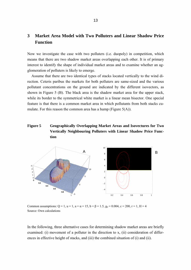
3 Market Area Model with Two Polluters and Linear Shadow Price Function
Now we investigate the case with two polluters (i.e. duopoly) in competition, which means that there are two shadow market areas overlapping each other. It is of primary interest to identify the shape of individual market areas and to examine whether an ag-glomeration of polluters is likely to emerge.
Assume that there are two identical types of stacks located vertically to the wind di-rection. Ceteris paribus the markets for both polluters are same-sized and the various pollutant concentrations on the ground are indicated by the different isovectors, as shown in Figure 5 (B). The black area is the shadow market area for the upper stack, while its border to the symmetrical white market is a linear mean bisector. One special feature is that there is a common market area in which pollutants from both stacks cu-mulate. For this reason the common area has a hump (Figure 5(A)). Figure 5 Geographically Overlapping Market Areas and Is vectures for Two
Vertically Neighbouring Polluters with Linear Shtion
00.2
0.40.6
0.8
1 - 5
0
5
10
0123
4
00.2
0.40.6
0.8
0.2 0.4 0.6
- 4
- 2
0
2
4
6
8
10
Common assumptions: Q = 1, u = 1, a = α = 15, b = β = 1.5, g0 = 0.004, c = 200, r Source: Own calculations In the following, three alternative cases for determining shadow marexamined: (i) movement of a polluter in the direction to x, (ii) conences in effective height of stacks, and (iii) the combined situation o
o
adow Price Func- A0.8 1
= 1, H = 4
ket areas are sideration of f (i) and (ii).
B
briefly differ-

14
Figure 6 shows, ceteris paribus, the effects of movement of a stack to the wind direc-tion. Since the shadow market areas of a pollutant are same-sized but shell-shaped, such an action creates a new boundary condition for the two market areas. They are con-nected by a hyperbolic arc. An increase in H of a stack generally leads to the change in pollution concentration and distribution pattern of pollutants on the ground at the same time. As a consequence, the shadow market area becomes smaller as H grows higher (Figure 7). Finally Figure 8 illustrates the case in which the second polluter with a higher stack is located within the shadow market area of the first polluter with a lower stack.
Figure 6 Geographically Overlapping Market Areas and Isovectures for Two Diagonally Neighbouring Polluters with Linear Shadow Price Func-tion
00.2
0.40.6
0.8
1 - 5
0
01234
00.2
0.40.6
0.8
10
Common assumptions: Q = 1, u = 1, a = αSource: Own calculations
A
5
10
0.2 0.4 0.6 0.8 1
- 4
- 2
0
2
4
6
8
= 15, b = β = 1.5, g0 = 0.004, c = 200, r = 1, H = 4
B

15
Figure 7 Geographically Overlapping Market Areas and Isovectures for Two Vertically Neighbouring Polluters with Linear Shadow Price Func-tion but Different Stack Heights
00.2
0.40.6
0.81 - 5
0
5
10
012
3
00.2
0.40.6
0.80.2 0.4 0.6 0.8 1
- 4
- 2
0
2
4
6
8
10
A B
Common assumptions: Q = 1, u = 1, a = α = 15, b = β = 1.5, g0 = 0.004, c = 200, r = 1, H1 = 4, H2 = 6 Source: Own calculations Figure 8 Geographically Overlapping Market Areas and Isovectures for Two
Horizontally Neighbouring Polluters with Linear Shadow Price Function but Different Stack Heights
00.2
0.40.6
0.81 - 5
0
5
10
0
1
2
3
00.2
0.40.6
0.80.2 0.4 0.6 0.8 1
- 4
- 2
0
2
4
6
8
10
Common assumptions: Q = 1, u = 1, a = α = 15, b = β = 1.5, g0 = 0.004, c = 200, r = 1, H1 = 4, HSource: Own calculations
B
A2 = 6

16
Figures 5 to 8 suggest that since the shape of the shadow market area is shell-shaped, the market boundary of two polluters can be a linear bisector or a hyperbolic arc, de-pending on their locations but regardless of their sizes. In particular a linear mean bisec-tor exists only when two same-sized market areas are overlapping each other vertically. This fact in turn expels the possibility of emerging the classical hexagonal market areas when many producers with the same-sized market areas prevail beside each other.
With the pollutant distribution function for two polluters f1(x, y) and f2(x, y), a con-sumer who is living in the common market area can ask for the compensation of the cumulated health hazard
(16) In the case of adopting a linear price function the condition shown in equation (16) ap-plies
(17) Consequently the customer living in the common area receives Pl(f1(x, y) from the pol-luter 1 and Pl(f2(x, y)) from the polluter 2. If this price linearity is transferred to the cal-culation of total compensation sum for the common market area A1∩A2
(18) The equation (18) also implicitly suggests that if a stack owner increases its Q and/or reduces H of its stack, then the shadow price for both polluters grows in the common market area, and vice versa. Once again, when the compensation payment for health hazard is assumed to be proportionally increasing with the pollutant concentration, the stack owners already existing in the market are indifferent regarding the competitive pressure or penetration of others. In this case the newcomers should additionally pay for shadow price for their own pollution activity in the common market area, which does not change the total payment sum of those already existing polluters at all.

17
4 Implication on Polluters’ Location Decision For the purpose of examining the issues surrounding the agglomeration of polluters or vice versa a quadratic shadow price function is adopted the character of which is com-parable to that of an exponential function. Such a type of function also expresses a pro-gressively growing relationship of the health hazard of consumers (and its compensa-tion) with the pollutant concentration level. Moreover, the quadratic function appears to be suitable to analytically demonstrate the additional costs caused by the overlap of shadow market areas of different polluters.
The price linearity in the common market areas of both polluters is not applicable for the case with an exponential price function, which means
(19) This fact is also well indicated in Figure 9, since the hump is extremely high for the common area and its slope is much steeper compared to the case with the linear price function in Figure 5. This fact clearly indicates that the individual payments of polluters in terms of Pe(fi(x, y)), i = 1, 2. to compensate the corresponding health hazard of con-sumers in this area is higher than the case with a linear price function. Figure 9 Geographically Overlapping Market Areas and Isovectures for Two
Vertically Neighbouring Polluters with Exponential Shadow Price Function
00.2
0.40.6
0.81 - 5
0
5
10
02468
00.2
0.40.6
0.80.2 0.4 0.6 0.8 1
- 4
- 2
0
2
4
6
8
10
A B
Common assumptions: Q = 1, u = 1, a = α = 15, b = β = 1.5, g0 = 0.004, c = 200, r = 1, H = 4 Source: Own calculations

18
We redisplay the quadratic shadow price function already mentioned in the box:
(20) Let us recall that P2 is designed to grow progressively starting with the value r at level g0 and with a first derivative equal to c in g0.
Compared to the case of monopoly, the extra compensation costs of polluter 1 which are caused by sharing a part of geographic market segment with polluter 2 can be ex-pressed locally by the function
(21) Not surprisingly, d(x,y) is positive as long as f2(x,y) is positive,
(22) In other words such a type of market sharing with the second polluter leads to additional compensation costs for polluter 1. If q > g0, for example, equation (21) can be rear-ranged by an explicit calculation to illustrate that
(23) Consequently, the total additional compensation costs for polluter 1 (Z1) which are caused by the common market area with polluter 2 amounts to
(24) In Figure 10 we show an explicit example. In the case of additionally applying the pa-rameter constellation with r = 1, c = 1000, g0 = 0.004 and H = 4, one obtains

19
(25)
arket. On the other hand, with a second polluter the costs for polluter 1 change to
(28)
ter 2 into the market amount to
(27)
igure 10 Market Areas for One Polluter vs. Two Polluters with Quadratic Shadow Price Function
for the total compensation costs for polluter 1 in Figure 10 (A), if he is alone in the m
(26) In our example the extra compensation costs for polluter 1 due to the penetration of pol-lu
Ceteris paribus the same logic applies also to the second polluter. F
00.2
0.40.6
0.81 - 10
- 5
0
05
10
15
00.2
0.40.6
0.8
B
Common assumptions: Q = 1, u = 1, a = α =
ource: Own calculations S
A
5
10
15
00.2
0.40.6
0.81 - 10
- 5
0
505
10
15
00.2
0.40.6
0.8
15, b = β = 1.5, g0 = 0.004, c = 1000, r = 1, H = 4.
10
15

20
As shown above, the market overlap creates extra compensation costs for both polluters hen assuming the super-linear shadow price function. This finding once again high-
onclusion
tifies the shadow market area of air pollutants based on the Gaussian lume model. Unlike the case for the classical theory of market area, transportation cost
in
wlights the fact that the penetration of a newcomer would hardly occur in an established market area of pollutants, since this action would make him and the existing polluter worse off. A sort of concentration of polluters would take place in the limited extent to which the market area of a stack owner directly borders that of others. C This study idenpdoes not play any role for its establishment, since pollutants are dispersed by the wind. Pollutant distribution on the ground level has an asymmetric bell-shape in the wind di-rection and is affected by parameters like stack height, wind force, etc. Such a type of distribution also correspondingly determines the two- and three-dimensional shape of market areas. In addition to the linear and the super-linear, the exponential shadow price function is also considered for the compensation of health hazard for the breathers of polluted air under the assumption that the strict liability based on the typical polluter-pays principle applies in the framework of Coase theorem. The compensation is de-pendent upon the concentration degree of pollutants on the ground. No amendment is made regarding the classical determinants for market areas like an isotropic surface and evenly distributed inhabitants with the same purchasing power and preference. In this case the shadow market area for the pollutants is not a circle but shell-shaped.
Such a shell-shaped market area has further distinct implications for the market boundaries between stack owners and their location decisions. In part the model find-
gs of the study refute the conventional wisdom related to this matter. They include: (1) the producers of pollutants are not located at the centre of their market areas and the market expansion is mainly possible in one direction, (2) since the shadow market area of an isolated polluter is shell-shaped, the market boundary of two polluters can be a linear bisector or a hyperbolic arc, depending on their locations, regardless of their sizes, and (3) the market overlap creates extra compensation costs for both polluters in the case of assuming the super-linear and exponential shadow price functions. Apart from expelling the possibilities of emerging traditional hexagonal market areas, all these facts also indicate that the penetration of a newcomer with a lower price would hardly occur in an established market area, and, that the agglomeration of polluters would take

21
place to the limited extent to which the market area of a stack owner just touches that of others. References
atabyal, A. A. and P. Nijkamp (2004), The Environment in Regional Science: An
Ba l.: Springer. licy, 2nd Edi-
Be interpretation, London and New
Be 972), Cournot Spatial Oligopoly, Papers of the Regional Science
Be heory, Berlin et al.: Springer. nd Flow,
Be Probleme der atmosphärischen Diffusion und der Ver-
Bo onmental Taxation and Regulation,
Br ition with Consumers on a Plane, at Intersec-
Br , Natural
Bu conomic Geography, New York et al.: John Wiley & Sons. ey, Eco-
Cs Diffusion in the Environment, Dordrecht and Boston:
Ch ansaction Costs and Environmental Policy: Institu-
B
Eclectic Review, Papers in Regional Science 83, 291-316. umbach, G. (1994), Luftreinhaltung, 3rd Edition, Berlin et a
Baumol, W. J. and W. E. Oates (1988), The Theory of Environmental Potion, Cambridge et al.: Cambridge University Press. avon, K. S. O. (1977), Central Place Theory: A ReYork: Longman. ckmann, M. J. (1Association 28, 37-47. ckmann, M. J. (1999), Lectures on Location T
Beckmann, M. J. and T. Puu (1985), Spatial Economics: Density, Potential aAmsterdam: North-Holland. rljand, M.E. (1982), Moderneschmutzung der Atmosphäre, Berlin: Akademie. venberg, A. L. and L. H. Goulder (2002), Envirin: Auerbach, A. J. and M. Feldstein (eds.), Handbook of Public Economics, Vol. 3, Amsterdam et al.: Elsevier, 1471-1545. aid, R. M. (1993), Spatial Price Compettions, and along Main Roadways, Journal of Regional Science 33, 187-205. omley, D. W. (1986), Markets and Externalities, in: Bromley, D. W. (ed.)Resource Economics: Policy Problems and Contemporary Analysis, Hingham, MA: Kluwer, 37-68. tler, J. (1980), E
Cansier, D. and R. Krumm (1997), Air Pollutant Taxation: An Empirical Survlogical Economics 23, 59-70. anady, G.T. (1972), TurbulentD. Reidel Publishing Company. allen, R. (2000), Institutions, Trtional Reform for Water Resources, Cheltenham: Edward Elgar.

22
Christaller, W. (1933), Die zentrale Orte im Süddeutschland: Eine ökonomisch-geographische Untersuchung über die Gesetzmäßigkeit der Verbreitung und Ent-wicklung der Siedlungen mit städtischen Funktionen, Jena: Fischer.
Coase, R. H. (1960), The Problem of Social Cost, Journal of Law and Economics 3, 1-44.
Crane, S. E. and P. J. Welch (1991), The Problem of Geographic Market Definition: Geographic Proximity vs. Economic Significance, Atlantic Economic Journal 19/2, 12-20.
Cropper, M. L. and W. E. Oates (1992), Environmental Economics: A Survey, Journal of Economic Literature 30, 675-740.
Cukrowski, J. and M. M. Fischer (2000), Theory of Comparative Advantage: Do Trans-portation Costs Matter?, Journal of Regional Science 40, 311-322.
Dasci, A. and G. Laporte (2004), Location and Pricing Decisions of a Multistore Mo-nopoly in a Spatial Market, Journal of Regional Science 44, 489-515.
Deaton, A. and J. Muellbauer (1980), Economics and Consumer Behaviour, Cambridge: Cambridge University Press.
Dixit, A. and M. Olson (2000), Does Voluntary Participation Undermines the Coase Theorem, Journal of Public Economics 76, 309-335.
Drezner, T. and Z. Drezner (1996), Competitive Facilities: Market Share and Location with Random Utility, Journal of Regional Science 36, 1-15.
Drezner, Z. and G. O. Wesolowsky (1996), Location-Allocation on a Line with De-mand-Dependent Costs, European Journal of Operation Research 90, 444-450.
Eskeland, G. S. (1994), A Presumptive Pigouvian Tax: Complementing Regulation to Mimic an Emission Fee, The World Bank Economic Review 8, 373-394.
Falconer, K., P. Dupraz and M. Whitby (2001), An Investigation of Policy Administra-tive Costs Using Panel Data for the English Environmentally Sensitive Areas, Jour-nal of Agricultural Economics 52, 83-103.
Fetter, F. A. (1924), The Economic Law of Market Areas, Quarterly Journal of Eco-nomics 38, 520-529.
Fik, T. (1991), Price Competition and Node-Linkage Association, Papers in Regional Science 7, 53-69.
Gustafsson, B. (1998), Scope and Limits of the Market Mechanism in Environmental Management, Ecological Economics 24, 259-274.
Heinsohn, R.J. and R.L. Kabel (1999), Sources and Control of Air Pollution, Upper Saddle River, NJ: Prentice Hall.
Hyson, C. D. and W. P. Hyson (1950), The Economic Law of Market Areas, Quarterly Journal of Economics 64, 319-327.

23
Kaplow, L. and S. Shavell (2002), Economic Analysis of Law, in: Auerbach, A. J. and M. Feldstein (eds.), Handbook of Public Economics, Vol. 3, Amsterdam et al.: El-sevier, 1661-1784.
Kohlberg, E. and W. Novshek (1982), Equilibrium in a Simple Price-Location Model, Economic Letters 9, 7-15.
Koop, G. and L. Tole (2004), Measuring the Health Effects of Air Pollution: To What Extent Can We Really Say That People Are Dying from Bad Air?, Journal of Envi-ronmental Economics and Management, 47, 30-54.
Lösch, A. (1940), Die räumliche Ordnung der Wirtschaft, Jena: Fischer. Maier, G. and F. Tödtling (1995), Regional- und Stadtökonomik: Standorttheorie und
Raumstruktur, 2nd Edition, Vienna and New York: Springer. McCann, L., B. Colby, K. W. Easter, Kasterine, A. and K. V. Kuperan (2004), Transac-
tion Cost Measurement for Evaluating Environmental Policies, Ecological Econom-ics 52, 527-542.
Melli, P. and E. Runca (1979), Gaussian Plume Model Parameters for Ground-Level and Elevated Sources Derived from the Atmospheric Diffusion Equation in a Neutral Case, Journal of Applied Meteorology: Vol. 18, 1216–1221.
Ohta, H. (1988), Spatial Price Theory of Imperfect Competition, Austin: Texas A&M University Press.
Palander, T. (1935), Beiträge zur Standortstheorie, Stockholm: Almquivst and Wick-sell.
Parr, J. B. (1995), The Economic Law of Market Areas: A Further Discussion, Journal of Regional Science 35, 599-615.
Petrakis, E. and A. Xepapadeas (2003), Location Decisions of a Polluting Firms and the Time Consistency of Environmental Policy, Resource and Energy Economics 25, 197-214.
Ponsard, C. (1983), A History of Spatial Economic Theory, Berlin: Springer. Praag van, B. M. S. and B. E. Baarsma (2000), The Shadow Price of Aircraft Noise Nui-
sance, Tinbergen Institute Discussion Paper 00-004/3. Puu, T. (2004), On the Genesis of Hexagonal Shapes, CERUM Working Papers 73,
Umeå University, Umeå. Schätzl, L. (1992), Wirtschaftsgeographie 1 (Theorie), Paderborn et al.: Schöningh. Schwartz, J. and R. Repetto (2000), Nonseparable Utility and the Double Dividend De-
bate: Reconsidering the Tax-interaction Effect, Environmental and Resource Eco-nomics 15, 149-157.
Shavell, S. (1984), Liability for Harm versus Regulation of Safety, Journal of Legal Studies 13, 357-374.

24
Sheshinski, E. (2004), On Atmosphere Externality and Corrective Taxes, Journal of Public Economics 88, 727-734.
Shaik, S., G. A. Helmers and M. R. Langmeier (2002), Direct and Indirect Shadow Price and Cost Estimates of Nitrogen Pollution Abatement, Journal of Agricultural and Resource Economics 27, 420-432.
Siebert, H. (1981), Praktische Schwierigkeiten bei der Steuerung der Umweltnutzung über Preise, in: Wegehenkel, L. (ed.), Marktwirtschaft und Umwelt, Tübingen: J. C. B. Mohr (Paul Siebeck), 28-53.
Siebert, H. (1992), Economics of Environment: Theory and Policy, 3rd Edition, Berlin et al.: Springer.
Söderholm, P. and T. Sundqvist (2003), Pricing Environmental Externalities in the Power Sector: Ethical Limits and Implications for Social Choice, Ecological Eco-nomics 46, 333-350.
Sutton, O.G. (1953), Micrometeorology, New York: McGraw-Hill. Turner, D.B. (1994), Workbook of Atmospheric Dispersion Estimates: An Introduction
to Dispersion Modelling, 2nd Edition, Boca Raton, Florida: Lewis Publishers. Uimonen, S. (2001), The Insufficiency of Pigouvian Taxes in a Spatial General Equilib-
rium Model, Annals of Regional Science 35, 283-298. Weber, A. (1909), Über den Standort der Industrie, Tübingen: J. C. B. Mohr (Paul
Siebeck). Wegehenkel, L. (1980), Coase Theorie und Marktsystem, Tübingen: J. C. B. Mohr (Paul
Siebeck). Williams, R. C. (2003), Health Effects and Optimal Environmental Taxes, Journal of
Public Economics 87, 323-335. Wong, S.-C. and H. Yang (1999), Determining Market Areas Captured by Competitive
Facilities: A Continuous Equilibrium Modeling Approach, Journal of Regional Sci-ence 39, 51-72.
Zannetti, P. (1990), Air Pollution Modeling-Theories, Computational Methods and Available Software, New York: Van Nostrand Reinhold.