1

Set-membership Identification and Fault Detection using a Bayesian

Framework

Rosa M. Fernández-Cantí, Joaquim Blesa, Vicenç Puig and Sebastian Tornil-Sin

Advanced Control Systems Group (SAC)

Universitat Politècnica de Catalunya (UPC), Pau Gargallo 5, 08028 Barcelona, Spain

Institut de Robòtica i

Informàtica Industrial, CSIC-UPC, Llorens i Artigas, Barcelona, Spain

e-mail: rfernandez@tsc.upc.edu, {joaquim.blesa,vicenc.puig,sebastian.tornil}@upc.edu

Abstract— This paper deals with the problem of set-membership identification

and fault detection using a Bayesian framework. The paper presents how the set-

membership model estimation problem can be reformulated from a Bayesian

viewpoint in order to, firstly, determine the feasible parameter set in the

identification stage and, secondly, check the consistency between the

measurement data and the model in the fault detection stage. The paper shows

that, assuming uniform distributed measurement noise and uniform model prior

probability distributions, the Bayesian approach leads to the same feasible

parameter set than the well-known set-membership technique based on

approximating the feasible parameter set using sets. Additionally, it can deal with

models that are nonlinear in the parameters. The single output and multiple

output cases are addressed as well. The procedure and results are illustrated by

means of the application to a quadruple tank process.

Keywords— Set-membership identification, fault detection, likelihood function,

Bayes rule

1. Introduction

In the Control Engineering field, the so-called Robust Identification techniques deal

2

with the problem of obtaining not only a nominal model of the plant, but also an

estimate of the uncertainty associated to the nominal model. Such model of uncertainty

is typically characterized as a region in the parameter space or as an uncertainty band

around the frequency response of the nominal model.

Uncertainty models have been widely used in the design of robust controllers (Sánchez

Peña and Sznaier, 1998) and, recently, their use in model-based fault detection

procedures is increasing (Chen and Patton, 1999; Reppa and Tzes, 2011). In this later

case, consistency between the new measurements and the parameter uncertainty region

is checked. When an inconsistency is found, the existence of a fault is decided.

There exist two main approaches to characterize model uncertainty: the

deterministic/worst case methods and the stochastic/probabilistic methods. For a survey,

see e.g. (Reinelt, Garulli, and Ljung, 2002). Deterministic methods lead to hard bounds

on the uncertainty region and the most representative are the set membership (SM)

techniques (Milanese and Taragna, 2002; Milanese and Taragna, 2005) and the

deterministic versions of the model error modelling (MEM) approach (Garulli and

Reinelt, 2000).

Stochastic methods such as the Non Stationary Stochastic Embedding (NSSE)

(Goodwin, Braslavsky, and Seron, 2002) lead to probabilistic bounds on the uncertainty

region. In early years, probabilistic bounds were considered not suitable to describe

uncertainty regions, but recent advances in robust risk adjusted controllers (Lagoa and

Sznaier, 2005) and probabilistic fault detection (Jaulin, 2010) have given raise to

stochastic methods. In particular, there is a renewed interest for the Bayesian point of

view in system identification (Ninness and Henriksen, 2010; Schön, Wills, and Ninness,

2011). The topic is not new since early works in system identification already

3

considered the Bayesian parameter estimation problem (Eykhoff, 1974) and model

classification problem (Peterka, 1981). Moreover, the relationship between

deterministic methods and stochastic methods was already explored in (Ninness and

Goodwin, 1995) on the basis of Bayesian estimation. However, the Bayesian ideas,

although appealing, have largely not been implemented due to the difficulty of

computing the integrations involved in the posterior distributions. Recent advances in

simulation techniques such as the Markov chain Monte Carlo (MCMC) have overcome

this situation (Bolstad, 2010). In this sense, particle filtering is widely used in situations

when state estimations are required (Arulampalam et al., 2002) and it is also applied in

fault diagnosis problems (Verma et al., 2004). In this paper, we focus on the problem of

set-membership parameter estimation for fault detection purposes, letting the extension

to state estimation (as its relation with particle filters) as future research.

The aim of the paper is to present how the set-membership model estimation problem

can be reformulated such that the Bayesian framework can be used to characterize the

feasible parameter set (FPS) and to check the consistency between the measurement

data and the model for fault detection purposes. Moreover, the proposed set-

membership Bayesian approach is compared with the deterministic set-membership

approach (Milanese, 1996) discussing the advantages and disadvantages of both

approaches. The paper shows that the Bayesian approach, assuming uniform distributed

measurement noise and uniform model prior probability distribution, leads to an inner

approximation of the FPS differently from the outer approximation provided by the set-

membership approach that uses sets to approximate the FPS. The motivation for using

the Bayesian methodology to solve set-membership estimation problem is that it can

deal with dynamic models that are nonlinear in the parameters. On the other hand, the

resulting FPS obtained with fault free data can be used for fault detection purposes

4

checking the consistency of the FPS with new data (Blesa, Puig, and Saludes, 2012). If

there is an inconsistency with new data and the FPS, a fault is present in the system, and

reinitializing the FPS to a large enough set, change in the healthy parameters can be

determined as was proposed in (Ingimundarson et al, 2009).

This paper is organized as follows: Section 2 establishes the model parameterization

that is going to be used and formulates the parameter set estimation problem and the

fault detection problem. Section 3 addresses the two problems from a Bayesian

viewpoint. In particular, we define the so-called Bayesian credible model set and

particularize it in order to solve the set-membership parameter estimation problem. We

also derive a test to check for faults on the basis of the resulting feasible parameter set.

Section 4 illustrates the application of the proposed method to a quadruple tank process

and presents the results in both the linear and the nonlinear cases. Finally, Section 5

concludes the paper.

2. Problem Definition

2.1. Model parameterization

Let us assume that the system can be expressed by means of the following regression

model for

ˆ( ) ( , ) ( ) ( , ) ( ) , 1,...,y k F k e k y k e k k M θ θ (1)

where ( , )F k θ is the regression (or observation) function, which in a general case is

assumed to be nonlinear in the parameters θ , and it can contain any function of the

5

system inputs ( )u k and outputs ( )y k , where k is the discrete time sample. The

regression function can be viewed as the estimate of the system response produced by

the model with parameters θ , ˆ( ) ( , )y k F k θ . oθ Θ is the parameter vector of

dimension 1n . oΘ is the set in the parameter space whose boundary represents the a

priori bounds for the parameter values. ( )e k is an additive error term which is unknown

but it is assumed to be bounded by a constant ( )e k .

Remark 1: Model parameterization (1) is introduced in order to better formalize the

proposed Bayesian set-membership approach and to allow a comparison with set-based

set-membership approaches (Milanese, 1996) that use the same type of

parameterization.

2.2. Parameter estimation problem

Given a sequence of input and output data (rich enough from the identificability point of

view and without no faults and outliers) collected from the system defined as

1,...,( )M k M

y y k

, 1,...,( )M k M

u u k

the parameter estimation problem can be defined as follows:

Definition 1: Given the system input and output sequences ( My , Mu ), the system model

expressed in regressor form (1), the noise bound and the initial parameter set oΘ ,

the set-membership parameter estimation problem consists in determining the Feasible

Parameter Set (FPS) defined as the set of parameters θ such that satisfy

( ) ( , ) , 1, , , oy k F k k M θ θ Θ

The FPS can be defined in compact form as follows

6

FPS | ( ) ( , ) ( ) , 1, ,o y k F k y k k M θ Θ θ (2)

In the case that the regression function is expressed linearly as ( , ) ( )TF k kθ φ θ , the

model parameterization (1) can be expressed as

ˆ( ) ( ) ( ) ( ) ( )Ty k k e k y k e k φ θ (3)

where ( )T kφ is the regressor vector of dimension 1 n . In this case, if the bound

parameter set oΘ is described by a convex polytope that can be expressed in the -

polytope form (Ziegler, 1995) as 0 0n

o Θ θ | A θ b with 0

nxnA and 0nb

the FPS is also a convex polytope (Blesa, Puig, and Saludes, 2012) that can be

described in the -polytope form as

0 0FPS n

A bθ | θ

A b

(4)

with

2

(1)

(1)

( )

( )

T

T

M n

T

T

M

M

φ

φ

A

φ

φ

, 2

(1)

(1)

( )

( )

M

y

y

y M

y M

b (5)

Also, in the linear regression case, the FPS can be obtained by intersecting all the M

strips defined by the pairs of parallel lines ( ( ) ( )Ty k k φ θ and ( ) ( )Ty k k φ θ

separated by 2 . In the case that the regression function ( , )F k θ is nonlinear in the

parameters θ , the resulting FPS is no longer a convex polytope but a region with a

much more complicated shape.

In order to avoid dealing with the exact description of the FPS several algorithms exist

7

that obtain inner or outer simpler regions that approximate the exact FPS. Such regions

are known as Approximated Feasible Parameter Sets (AFPS).

Inner approximations find the approximate parameter set of maximum volume AFPSin

such that all its parameters are inside the feasible parameter set,

AFPS FPSin . (6)

On the other hand, outer approximation algorithms find the approximate parameter set

of minimum volume AFPSout that guarantees that the feasible parameter set is inside it,

FPS AFPSout . (7)

When ( , )F k θ is linear, boxes, parallelotopes, ellipsoids or zonotopes are used to

characterize the AFPS (Alamo, Bravo, and Camacho, 2005; Blesa, Puig, and Saludes,

2011). In the nonlinear case, a minimum outer box can be determined by means of a set

of optimization problems (Milanese et al., 1996). But since the parameters enter in a

nonlinear way in (1), the resulting optimization problems are nonconvex.

As an alternative to nonconvex optimization, recursive algorithms can be used as

follows

FPS( )=FPS( 1) S( )k k k (8)

where S(k) is the set of parameters consistent with data at the sample k

S( ) | ,nk y k F k θ θ (9)

Recursive algorithms allow the efficient computation of inner

AFPS ( ) AFPS ( 1) S( )in ink k k (10)

8

or outer approximations

AFPS ( 1) S( ) AFPS ( )out outk k k (11)

In this latter approach, the AFPS can be estimated by using subpavings and the SIVIA

(Set Inversion Via Interval Analysis) algorithm which is based on refining the initial a

priori set oΘ by iteratively bisecting it (Jaulin, Kieffer, Didrit, and Walter, 2001).

2.3. Fault detection in the set-membership framework

Once the FPS (or its approximation) has been estimated with nonfaulty data, it can be

used for fault detection.

The fault detection problem in the set-membership can be defined as follows:

Definition 2: Given the system input and output sequences ( My , Mu ), the system model

expressed in regressor form (1), the noise bound and the initial parameter set oΘ ,

the set-membership fault detection problem consists in determining if

FPS | ( ) ( , ) ( ) , 1, ,o y k F k y k k M θ Θ θ

to prove the inconsistency between the input/output data and the model. In the

inconsistency is proved, a fault is indicated.

The fault detection test can be implemented in a recursive way by checking if the set of

parameters consistent with data at the sample k (9) is inconsistent with the FPS. The

inconsistency can be checked by means of the intersection of S(k) with the FPS. A fault

will be indicated if this intersection leads to an empty set

S( ) FPSk (12)

In the linear case, if the identification data length is moderate, the fault detection test

9

(12) can be solved efficiently by determining the feasibility of a linear optimization

problem.

2.4. Extension to the multiple output case

The previous results can be extended to the case of multiple outputs. Consider now that

system to be monitored can be expressed by means of the following multiple output

regression model

ˆ( ) ( , ) ( ) ( , ) ( ) , 1,...,k k k k k k M y F θ e y θ e (13)

where the vector regression function ( , )kF θ can be nonlinear in the parameters θ , and it

contains any function of vector inputs ( )ku and outputs ( )ky and can be decomposed in

ny components 1( , ) ( , ), , ( , )y

T

nk F k F kF θ θ θ in such a way that

1 1 1 1 1ˆ( ) ( , ) ( ) ( , ) ( )

ˆ( ) ( , ) ( ) ( , ) ( )y y y y yn n n n n

y k F k e k y k e k

y k F k e k y k e k

θ θ

θ θ

(14)

where 1( ), , ( )nyy k y k are the ny components of the output vector ( )ky and 1( ), , ( )nye k e k

are the ny components of the additive error vector ( )ke which is unknown but it is

assumed to be bounded by a constant ( ) , ,i ie k k 1, , yi n .

Now, the parameter set consistent to input/output data at sample k, S(k), is defined as

the intersection of the consistency sets corresponding to each output i, Si(k), i=1,…,ny,

at the same sample k

1S )S( ) (yn

iikk

(15)

with

10

|S ( ) ,i i i in

ik y k F k θ θ (16)

The set S(k) can be expressed in a compact form as follows

1 1 1 1,

S( )

,y y y y

n

n n n n

y k F k

k

y k F k

θ

θ

θ

(17)

In the same way, the FPS corresponding to the multiple output case is now

1

0

1 1 1,

,

FPS , 1,...,

y y y yn n n n

y k F k

y k F

k M

k

θ

θ

θ

(18)

As in the single output case, if the regression function ( , )kF θ is linear in the parameters

θ , the multiple output FPS can be described as a convex polytope. Thus, the set-

membership estimation and fault detection procedures described in the previous

sections for the single output case can be used for the multiple output case as well.

3. Set-membership Estimation and Fault Detection in the Bayesian Framework

Once the set-membership parameter estimation and fault detection problems have

introduced, an approach to solve them based on the Bayesian framework is proposed.

3.1. Bayesian set-membership parameter estimation

The parametric-type uncertainty can be described by means of the Bayesian credible

parameter set:

0 : ( ) ( )p c θ θ Θ θ yB (19)

11

where the process model is characterized by means of the parameter vector θ ,

TMyy )(...)1(y

is the measurement data vector, ( )c is the critical value where

100(1- )% is the desired credibility level, and the model posterior distribution can be

obtained by means of the Bayes’ rule,

( | , ) ( )( | )

( )

p pp

p

y θ θθ y

y (20)

where ( | , )p y θ is the likelihood of the observations y jointly conditioned to the model

θ and to the error bound , ( )p θ is the prior distribution on the model parameters, and

( )p y is just a normalized constant, so we can express the posterior as

( | ) ( | , ) ( )p p pθ y y θ θ .

Note that although the Bayesian credible parameter set (19) is a very general set suitable

for most identification procedures, including nonparametric and nonstandard

distributions, it is not necessary to use it in its full powerfulness for the parameter set

estimation problem considered here. A simpler version, obtained by taking the

assumptions that are listed below, will be enough.However, different assumptions

would lead to different types of AFPSs, some of them, characterized by more complete

descriptions of the posterior distribution, and surely enjoying different and interesting

properties, but for the sake of clearness here we focus on the simplest case.

Hence, the following assumptions allow showing that the FPS defined in Section 2 can

be approximated from a Bayesian approach. These assumptions lead to a point-wise

inner approximation of (2).

The assumptions taken in this work are the following:

12

First assumption: The prior distribution is uniform. In the Bayesian framework, the

model prior probability distribution ( )p θ can be a subjective probability (Robert,

2001). For simplicity, here it is assumed that no information about which the value of

the “true” parameter vector θ will be and consequently we take a uniform ( )p θ which

is flat over the initial set oΘ . This way the model posterior distribution is directly

proportional to the likelihood function of the observations, ( | ) ( | , )p p θ y y θ in the

considered initial support oΘ .

Since for a fixed θ , ˆ( ) ( , ),y k F k k θ , are deterministic quantities, the likelihood

( | , )p y θ coincides in form with the error term distribution, i.e., ˆ( | , ) |ep p y θ y y ,

where ˆ ˆ ˆ(1) ... ( )T

y y My .

Second assumption: The error term is uniform distributed. To obtain a hard-bounded

uncertainty region (credible region in the Bayesian terminology), we must assume that

the distribution of the additive error is hard-bounded. The simplest choice is to take the

uniform distribution, i.e., e(k)~U ( , ), k , where is selected to be the additive error

bound presented in Section 2. In this case, the resulting likelihood function is constant

and nonzero in the region where models θ are consistent with the measurements and it

is zero outside this region.

Note that, unlike particle filtering approaches (Arulampalam et al., 2002), we are not

really concerned on obtaining the posterior distribution for θ ; instead, what we obtain is

the region (within the initial support oΘ ) for which the posterior distribution for θ is

constant and nonzero. This region will serve as an inner characterization of the AFPS.

Note also that, since the value of the posterior distribution for θ is constant over the

13

FPS, the value is not relevant here either. All models θ will be equally probable to

occur, and the probability level will be related to the FPS size. If we were interested in

different levels of probability inside the hard-bounded FPS we could use different prior

distributions for θ , e.g. Gaussian distributions. Still, if we were interested in soft-

bounded FPSs we could use soft-bounded likelihood functions instead of uniform

likelihood functions. These two later situations are out of the scope of this paper and

will not be considered here.

Third assumption: Equation-error assumption. The likelihood function can be

numerically estimated by taking the so-called equation-error assumption. On the

contrary to the error-in-variables approach, where the regression function itself presents

an error term, the equation-error approach assumes that the error term is additive to the

data at each time sample k. This assumption was early justified in (Sorenson, 1970) and,

since it significantly simplifies the procedures, it is assumed in most set-membership

parametric techniques (Milanese et al., 1996).

This way, we can assume that the error samples ˆ( ) ( ) ( ),e k y k y k k are i.i.d.

(independent and identically distributed) and we can compute the likelihood function

numerically and sample-to-sample,

1

ˆ ˆ( | , ) ( ( ) ( ) | , )M

e ek

p p y k y k

y y θ θ (21)

Note that there is no difference in the computation of (21) whether ( , )F k θ �is linear in

the parameters or not. The likelihood function (21) can be numerically estimated by

using a Monte Carlo approach, see e.g. (Ninness and Henriksen, 2010; Schön et al.,

2010). This is the choice in most Bayesian works. However, in the next section, we

estimate it by means of the gridding of the candidate parameter vectors iθ and taking

14

the equation-error assumption.

3.2. Computation of the point-wise Bayesian AFPS

The approximation for the FPS in the Bayesian approach is the following:

AFPS | ( ) ( , ) | , 0, 1, , , 1,...,i o e i ip y k F k k M i N θ Θ θ θ B (22)

The simplest procedure to compute (22) consists in taking an arbitrary point grid in oΘ

defined by a pre-specified distance between points. Each point iθ corresponds to a

possible model for the physical plant. Then, for each time sample and model iθ , we

compute the error between the measurement and the predicted output ˆ( ) ( , )iy k F k θ . If

this error is inside the bound, we conclude that the model is consistent with the

measurements and we assign it a likelihood value of one, ˆ( ) ( ) | , 1e ip y k y k θ ;

otherwise, the likelihood is zero. This procedure is repeated for all M samples for all the

N points iθ in the grid.

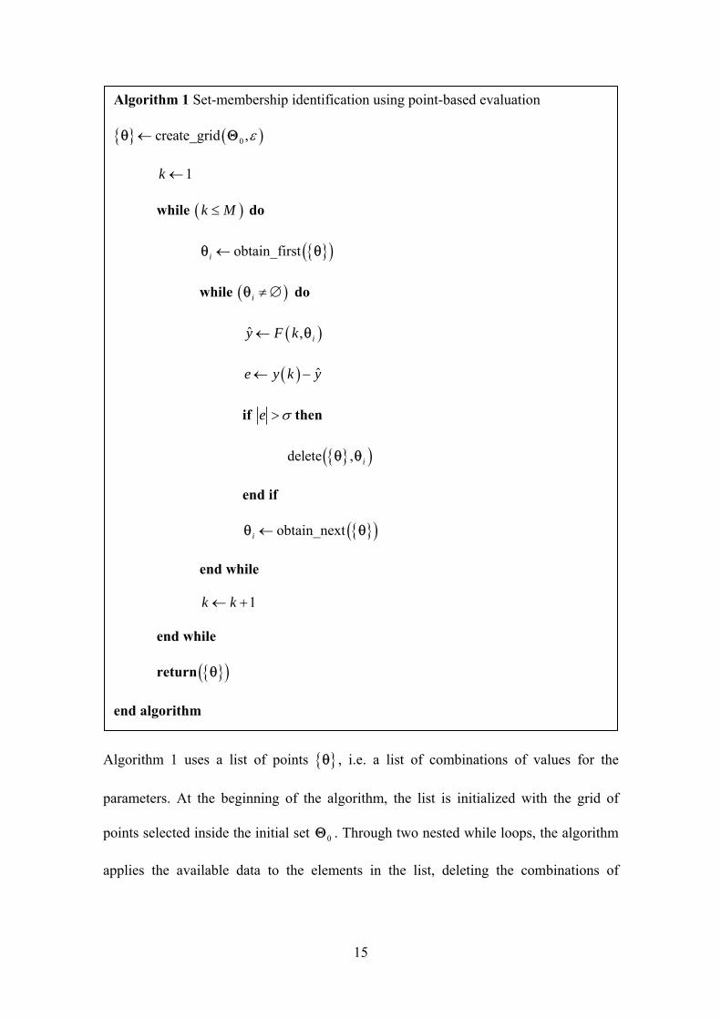
A high level description of the procedure is summarized in Algorithm 1.

15

Algorithm 1 uses a list of points , i.e. a list of combinations of values for the

parameters. At the beginning of the algorithm, the list is initialized with the grid of

points selected inside the initial set 0 . Through two nested while loops, the algorithm

applies the available data to the elements in the list, deleting the combinations of

Algorithm 1 Set-membership identification using point-based evaluation

0create_grid ,

1k

while k M do

obtain_firsti

while i do

ˆ , iy F k

ˆe y k y

if e then

delete , i

end if

obtain_nexti

end while

1k k

end while

return

end algorithm

16

parameters that are proven to be inconsistent with the data at any time instant. The

algorithm returns a list of points that belong to the FPS, hence providing an inner AFPS.

Remark 2: Since all the M observations in Algorithm 1 should be included in the output

prediction zonotope , the presence of exceptional data points (i.e., outliers) may lead to

empty or marginal FPS. In order to address this issue, algorithms to remove outliers

(like the ones proposed in Campi. Calafiore and Garatti, 2009) should be applied such

that oM M data are discarded and apply the remaining oM M data to Alogrithm 1.

3.3. Fault detection in the Bayesian framework

Once we have calibrated the Bayesian model (i.e., we have obtained the samples of the

likelihood function ˆ( | , )e ip y y θ for all the points iθ in the parameter grid), the

detection of faults can be carried out for every new measurement y(k), 1k M , by

computing the new likelihood function ˆ( ( ) ( ) | , ),e i ip y k y k θ θ , and verifying whether

there is at least one parameter vector jθ in the grid for which both the calibrated

likelihood ˆ( | , )e jp y y θ and the new likelihood ˆ( ( ) ( ) | , ), 1e jp y k y k k θ , are

nonzero. If this parameter (or set of parameters) exists, we conclude that the new

measurement is consistent with the AFPS.

The consistency can be checked by simply multiplying both likelihood functions for

each parameter iθ in the grid. If the product is equal to zero for all the parameters in the

grid,

ˆ ˆ( | , ) ( ( ) ( ) | , ) 0, , 1e i e i ip p y k y k k M y y θ θ θ (23)

we decide that a fault has taken place. Since we consider a sample at once, the test (23)

17

can be implemented on-line by means of Algorithm 2.

Algorithm 2 Set-membership fault detection using point-based evaluation

AFPS B

1k

0FD

while k end do

obtain_firsti

while i do

ˆ , iy F k

ˆe y k y

if e then

delete , i

end if

obtain_nexti

end while

if is_empty then

1FD

0create_grid ,

end if

1k k

end while

end algorithm

18

Algorithm 2 for fault detection is a modification of Algorithm 1 for parameter

estimation. However, it must be noticed that both algorithms will be used under

different conditions: Algorithm 1 will be applied off-line using data collected for system

normal (fault-free) operation, while Algorithm 2 will be applied on-line with the goal of

determining the system condition in real-time. The differences with Algorithm 1 are the

following. First, in Algorithm 2 the initialization of the list of points in the parameter

space uses the results previously obtained by Algorithm 1. Second, if at any time

instant k the list of points becomes empty because none of the combinations of

parameters in the list is consistent with the data, then the fault indicator FD is set and

the list is reinitialized by using the a-priori initial parameter set 0 . This allows the

algorithm not only to detect faults but also to identify the magnitude for parametric

faults.

Of course, the ability to detect “small” faults depends on the grid density (the number

N of candidate parameter vectors iθ ) but it does not depend on c() in the hard-

bounded case considered here (since all the models inside the AFPS are equally

probable and the value would only assign the percentage of probability corresponding

to each of them). A denser grid would be able to detect smaller deviations of the

parameter vector, because more uncertain nonfaulty models would be checked in (23)

and thus we would have more models able to explain the normal behavior. Moreover, a

denser grid would also decrease the number of false alarms, since the borders of the

AFPS would contain more models able to explain the normal behavior. Although a

denser grid implies a more intense calibration stage, it does not increase significantly

the computation load in the fault detection stage.

19

3.4. Extension to the multiple output case

The uncertainty calibration procedure explained in the previous section can be extended

to the case of multiple output systems by taking the joint likelihood function of the ny

outputs

1 1 1 11

ˆ ˆ ˆ ˆ( ,..., | , ) ( ( ) ( ) | , ) ( ( ) ( ) | , )y y y y

M

e n n e e n nk

p p y k y k p y k y k

y y y y θ θ θ (24)

And the fault detection procedure can be generalized in an analogous way,

1 1 1 1ˆ ˆ ˆ ˆ( ,..., | , ) ( ( ) ( ) | , ) ( ( ) ( ) | , ) 0,

, 1y y y ye n n i e i e n n i

i

p p y k y k p y k y k

k M

y y y y θ θ θ

θ

(25)

3.5. Discussion

The mainstream in set-membership parameter estimation considers the use of set-based

methods. Typically, the result of a parameter estimation problem is a set of a given type

that provides an outer approximation (as accurate as possible) of the exact FPS. A rich

variety of approximating sets are proposed in the literature, e.g. boxes, ellipsoids,

polytopes, zonotopes and subpavings. Unfortunately, some of the previous types of sets

can only be used for the identification of linear systems. Boxes and subpavings,

manipulated by using interval analysis methods, are the only ones that can be used for

the identification of non-linear systems. And since boxes provide too rough

approximations for arbitrary shaped sets, subpavings are at the end the only alternative.

The standard set-based solution to the non-linear parameter estimation problem is the

use of subpavings and the SIVIA (Set Inversion Via Interval Analysis) algorithm (Jaulin

et al., 2001). Subpavings are unions of non-overlapping boxes that can approximate

compact sets with arbitrary precision. The SIVIA algorithm provides an (outer)

approximation of the subset of points in the domain whose evaluation by a given

20

function lies in a prespecified image set. The SIVIA algorithm can be directly applied to

the Set Membership parameter estimation problem, being the function to evaluate the

regression function ( , )F k θ in (1) and being the image set the box given by the addition

of the uncertainty to the measurements, i.e. , , 0, ,y k y k y k k M .

The proposed Bayesian Set Membership parameter estimation algorithm can be

compared with SIVIA. The first aspect to consider is that SIVIA provides outer

approximations of the exact FPS while the Bayesian method will provide inner

approximations. Applied to the fault detection problem, this means that SIVIA will

assure the elimination of false alarms but with a loss of sensitivity to faults. On the other

hand, the use of the Bayesian method will lead to a given false alarm rate different from

zero but without a loss of fault sensitivity (in fact, the sensitivity to faults will increase).

To decide if it is worse to loose fault sensitivity or to have false alarms may depend on

the application, but in general it depends on their magnitudes. And these magnitudes are

associated to the quality of the outer and inner approximations of the FPS provided by

the two methods. Both methods share the property of being able to provide

approximations of arbitrary precision at a cost of computation time, but their

performances can be compared working at fixed resolution levels. Some experiments

using an example and detailed in the previous work (Fernández-Canti et al., 2013)

suggest that for a given resolution level the quality of the inner approximation provided

by the Bayesian method is expected to be higher than the quality of the outer

approximation provided by SIVIA (excess of overbounding due to the well known

multi-incidence problem of interval arithmetic). On the other hand, the computation

time needed by the Bayesian method is expected to be lower than the needed by SIVIA.

21

4. Example

A quadruple-tank process, proposed by (Johansson, 2000), is used to illustrate the

procedures presented in this paper. The schematic diagram of the system is shown in

Figure 1. The process inputs are the input voltages to the pumps, 1v and 2v , and the

process outputs are the tank levels , 1, ,4ih i .

Figure 1. Quadruple-tank process

4.1. Multi input single output model

We firstly focus on a part of the whole system. We assume that the levels 1h , 3h and the

voltage 1v can be directly measured. The equation that describes the dynamic behavior

of this part of the system (output: h1, inputs: h3, v1) is:

31 1 11 1 3 1

1 1 1

2 2aa k

h gh gh vA A A

(26)

where 1 1 /h dh dt , a1 and a3 are the cross-sections of the outlet holes of tanks 1 and 3,

and 21 28cmA is the cross-section of tank 1. The term 1 1k v with 3

1 3.33 cm /Vsk is the first

22

pump flow and the parameter 1 0.7 is determined from how the first valve is set prior

to the experiment. The gravity acceleration is 2981cm/sg . Finally, we consider that

the operating range is 1 2,11 cmh and 3 1,15 cmh .

The parameters a1 and a3 are the ones to be estimated and their nominal values are

assumed to be 2

1 3 0.071a a cm .

4.2. Discrete models

Discrete models for the linear and nonlinear regression cases will be used to illustrate

that the proposed approach works well in either case:

4.2.1. Linear case

A discrete, linearized version of (26) can be obtained by means of the forward

approximation of the derivative 1 1 1( ( ) ( 1)) / sh h k h k T with sampling time 1sT s . This

way, (26) can be expressed in the following linear regression form

1 11 1 1

1

( ) ( 1) ( ) ( 1) ( )T kh k h k k v k e k

A

φ θ (27)

where 1 31 1

1 1( ) 2 ( 1) 2 ( 1)T k gh k gh k

A A

φ is the regressor vector and 1 3T

a aθ

is the model parameter vector to be estimated. The term ( )e k is the additive error due to

the measurement noise and discretization and it is assumed to be bounded,

( ) 0.05 cme k .

4.2.2. Nonlinear case

23

A model nonlinear in the parameters can be obtained if an output observer is used (see

Figure 2).

Figure 2. Multi Input Single Output plant with output observer

Observers improve the ability of detecting output faults but lead to structures nonlinear

in the parameters. In our example, the resulting expression is

1 11 1 1 1 1

1

ˆ ˆ ˆ( ) ( 1) ( ) ( 1) ( ) ( 1) ( 1)T kh k h k k v k e k L h k h k

A

φ θ (28)

where 1 31 1

1 1ˆ( ) 2 ( 1) 2 ( 1)T k gh k gh kA A

φ , 1 3T

a aθ , and ( ) 0.05 cme k .

4.3. Uncertainty estimation in a fault-free scenario

To obtain the uncertainty region (FPS), i.e., to determine the uncertainty region for a1

and a3 in the parameter space, a set of M=140 measurements has been obtained in a

fault-free scenario (see Figure 3).

24

0 20 40 60 80 100 120 1400

5

10

15

Levels h1 and h

3

Time (s)

cm

h1

h3

0 20 40 60 80 100 120 1400

0.5

1

Pump voltage v1

Time (s)

Vol

ts

Figure 3. Identification scenario

4.3.1. Linear case

Figure 4 shows the FPS obtained by the strips intersection set-membership technique

described in Section 2. The red little circles indicate the final (i.e., after M intersections)

polytope vertices.

0.065 0.07 0.075 0.080.065

0.07

0.075

0.08

a1

a 3

Feasible Parameter Set (strips intersection)

Figure 4. FPS obtained by the strips intersection technique

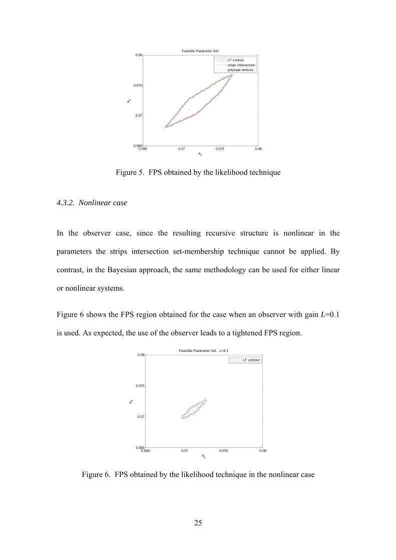
Figure 5 shows the FPS region obtained by computing the contour of the likelihood

function assuming that the error is uniform distributed as , U for a grid of 6060

parameters. As expected, this region coincides to the one obtained by the strips

intersection method shown in Figure 4.

25

a1

a 3

Feasible Parameter Set

0.065 0.07 0.075 0.080.065

0.07

0.075

0.08

LF contour

strips intersectionpolytope vertices

Figure 5. FPS obtained by the likelihood technique

4.3.2. Nonlinear case

In the observer case, since the resulting recursive structure is nonlinear in the

parameters the strips intersection set-membership technique cannot be applied. By

contrast, in the Bayesian approach, the same methodology can be used for either linear

or nonlinear systems.

Figure 6 shows the FPS region obtained for the case when an observer with gain L=0.1

is used. As expected, the use of the observer leads to a tightened FPS region.

a1

a 3

Feasible Parameter Set. L=0.1

0.065 0.07 0.075 0.080.065

0.07

0.075

0.08

LF contour

Figure 6. FPS obtained by the likelihood technique in the nonlinear case

26

4.4. Uncertainty estimation in a fault-free scenario for the MIMO case

Now we consider the MIMO (Multiple Input Multiple Output) case. A set of 21000

measurement data have been obtained for the whole system. Figure 7 shows the steady

state final 14000 samples for each tank level. The first 500M samples of this record

will be used for calibration purposes.

0 2000 4000 6000 8000 10000 12000 140000

10

20

h 1 (cm

)

0 2000 4000 6000 8000 10000 12000 140005

10

15

h 2 (cm

)

0 2000 4000 6000 8000 10000 12000 140001

2

3

h 3 (cm

)

0 2000 4000 6000 8000 10000 12000 140001

2

3

h 4 (cm

)

Time (s)

Figure 7. Measurement data for the MIMO case

The system in (26) can be viewed as two independent MIMO systems. In the first one,

the inputs are v1 and v2, and the outputs are h1 and h3. The uncertain parameters are,

again, a1 and a3.

31 1 1 11 3 1

1 1 1

2 2adh a k

gh gh vdt A A A

(29)

3 3 2 23 2

3 3

(1 )2

dh a kgh v

dt A A

(30)

In the second one, the inputs are v1 and v2, and the outputs are h2 and h4. The uncertain

27

parameters are a2 and a4.

2 2 4 2 22 4 2

2 2 2

2 2dh a a k

gh gh vdt A A A

(31)

4 4 1 14 1

4 4

(1 )2

dh a kgh v

dt A A

(32)

The identified error bounds are 1 0.1134 , 2 0.1098 , 3 0.1036 , and

4 0.1024 .

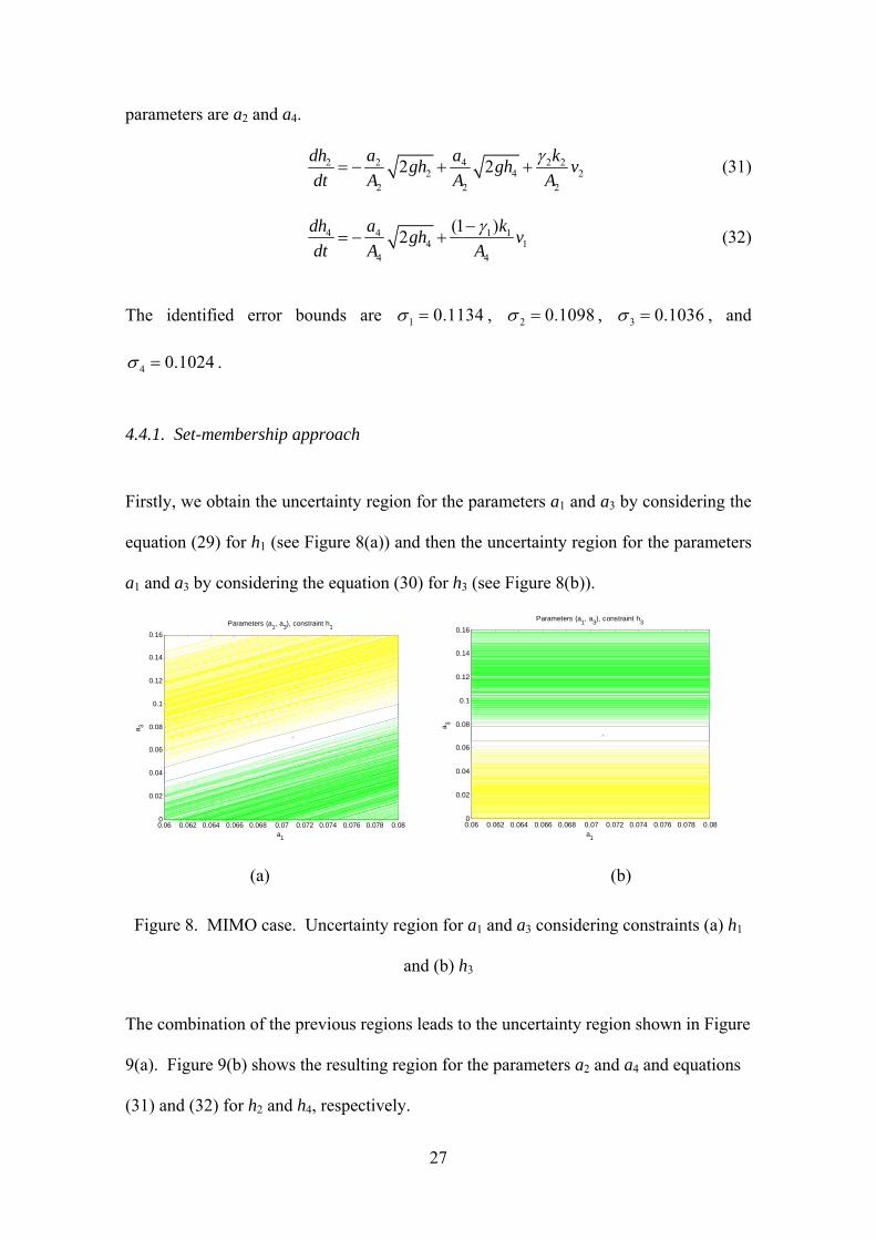
4.4.1. Set-membership approach

Firstly, we obtain the uncertainty region for the parameters a1 and a3 by considering the

equation (29) for h1 (see Figure 8(a)) and then the uncertainty region for the parameters

a1 and a3 by considering the equation (30) for h3 (see Figure 8(b)).

0.06 0.062 0.064 0.066 0.068 0.07 0.072 0.074 0.076 0.078 0.080

0.02

0.04

0.06

0.08

0.1

0.12

0.14

0.16

a1

a 3

Parameters (a1, a

3), constraint h

1

0.06 0.062 0.064 0.066 0.068 0.07 0.072 0.074 0.076 0.078 0.080

0.02

0.04

0.06

0.08

0.1

0.12

0.14

0.16

a1

a 3

Parameters (a1, a

3), constraint h

3

(a) (b)

Figure 8. MIMO case. Uncertainty region for a1 and a3 considering constraints (a) h1

and (b) h3

The combination of the previous regions leads to the uncertainty region shown in Figure

9(a). Figure 9(b) shows the resulting region for the parameters a2 and a4 and equations

(31) and (32) for h2 and h4, respectively.

28

0.06 0.062 0.064 0.066 0.068 0.07 0.072 0.074 0.076 0.078 0.080

0.02

0.04

0.06

0.08

0.1

0.12

0.14

0.16

a1

a 3

Parameters (a1, a3), constraints (h1, h3)

0.05 0.052 0.054 0.056 0.058 0.06 0.062 0.064 0.066 0.068 0.070

0.02

0.04

0.06

0.08

0.1

0.12

0.14

0.16

a2

a 4

Parameters (a2, a

4), constraints (h

2, h

4)

(a) (b)

Figure 9. MIMO case: (a) Final uncertainty region for a1 and a3 (b) Final uncertainty

region for a2 and a2

4.4.2. Likelihood approach

The same region shown in Figure 9(a) can be obtained by computing the likelihood to

obtain the measurements h1, h3 for each pair of parameters a1, a3,

1 3 1 3 1 1 1 1 3 3 3 3 1 31

( , | , ) ( | , ) ( | , )M

k

p h h a a p h h a a p h h a a

(31)

by taking a 30 30 parameters grid, and considering uniform probability distributions

for the residuals, 1 1 1 3 1 1( | , ) ( , )h h a a U : and 3 3 1 3 3 3( | , ) ( , )h h a a U : .

Figure 10 shows the results for M=500 and a grid of 80 80 values for a1, a3 ranging

from 0.06 to 0.08.

29

0.060.065

0.070.075

0.080.085

0.06

0.07

0.08

0.090

0.2

0.4

0.6

0.8

1

a1

FPS for (a1,a

3) with constraints (h

1,h

3)

a3

Like

lihoo

d fu

nctio

n

a1

a 3

FPS for (a1,a

3) with constraints (h

1,h

3)

0.064 0.066 0.068 0.07 0.072 0.074 0.076 0.078 0.080.06

0.065

0.07

0.075

0.08

0.085

LF contour

SM polytopetrue values

(a) (b)

Figure 10. MIMO case, parameters a1, a3. (a) normalized likelihood function, (b)

likelihood function contour plot.

Similar results are obtained for each pair of parameters a2, a4 by computing the

likelihood to obtain the measurements h2, h4 (see Figure 11).

0.05

0.06

0.07

0.08

0.05

0.06

0.07

0.080

0.2

0.4

0.6

0.8

1

a2

FPS for (a2,a4) with constraints (h2,h4)

a4

Like

lihoo

d fu

nctio

n

a2

a 4

FPS for (a2,a

4) with constraints (h

2,h

4)

0.052 0.054 0.056 0.058 0.06 0.062 0.0640.045

0.05

0.055

0.06

0.065

0.07 LF contour

SM polytopetrue values

(a) (b)

Figure 11. MIMO case, parameters a2, a4. (a) normalized likelihood function, (b)

likelihood function contour plot.

30

4.5. Fault detection results

In order to compare the performance of the strips intersection and likelihood fault

detection tests, different fault scenarios have been created by introducing faults when

the system is under the operation point shown in Figure 12. For the sake of clearness, in

this section we only consider the MISO (Multi Input Single Output) case.

0 200 400 600 800 1000 1200 1400 1600 1800

4

6

8

10

Time (s)

cm

Levels h1 and h3

h1

h3

0 200 400 600 800 1000 1200 1400 1600 1800 20000

0.5

1

Time (s)

Vol

ts

Pump 1 (v1)

Figure 12. No faulty scenario

Here we illustrate the case when a fault consisting of an additive constant of value 0.035

acting over the parameter 1a is introduced at the sample 1201. The faulty behavior is

shown in Figure 13.

0 200 400 600 800 1000 1200 1400 1600 1800 20001

2

3

4

5

6

7

8

9

10

Time (s)

cm

Level at tank 1

fault

no fault

Figure 13. Faulty scenario

Figures 14 and 15 illustrate the fault detection test for the set-membership technique

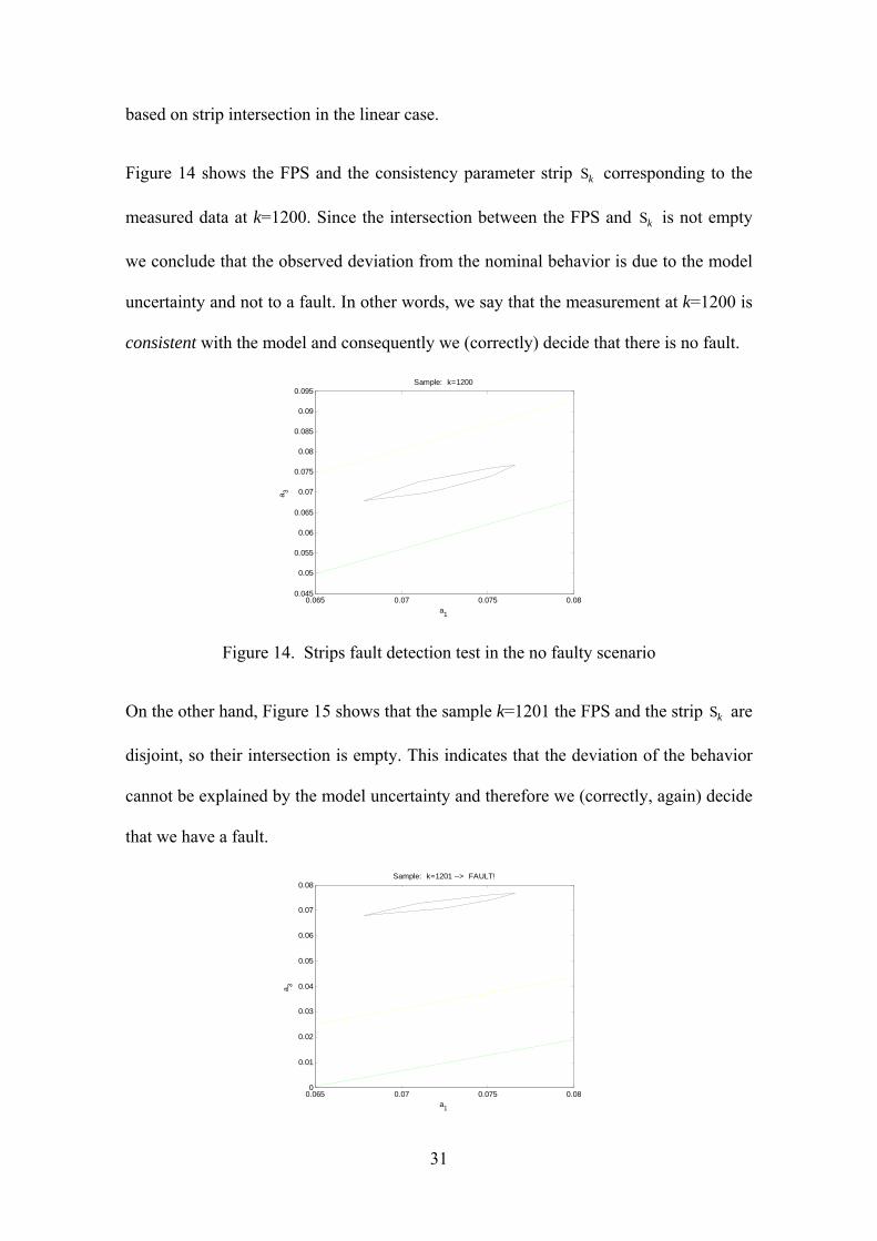
31

based on strip intersection in the linear case.

Figure 14 shows the FPS and the consistency parameter strip Sk corresponding to the

measured data at k=1200. Since the intersection between the FPS and Sk is not empty

we conclude that the observed deviation from the nominal behavior is due to the model

uncertainty and not to a fault. In other words, we say that the measurement at k=1200 is

consistent with the model and consequently we (correctly) decide that there is no fault.

0.065 0.07 0.075 0.080.045

0.05

0.055

0.06

0.065

0.07

0.075

0.08

0.085

0.09

0.095Sample: k=1200

a1

a 3

Figure 14. Strips fault detection test in the no faulty scenario

On the other hand, Figure 15 shows that the sample k=1201 the FPS and the strip Sk are

disjoint, so their intersection is empty. This indicates that the deviation of the behavior

cannot be explained by the model uncertainty and therefore we (correctly, again) decide

that we have a fault.

0.065 0.07 0.075 0.080

0.01

0.02

0.03

0.04

0.05

0.06

0.07

0.08Sample: k=1201 --> FAULT!

a1

a 3

32

Figure 15. Strips fault detection test when the fault occurs

Finally, Figure 16 and Figure 17 illustrate the likelihood fault detection test in the linear

case for a grid of 6060 parameters.

Figure 16 shows the initial likelihood function corresponding to the FPS and the

likelihood function computed for the new measurement at k=1200. The top value in

both functions has been scaled to 5 and 10 respectively for comparison purposes. In this

sample, the new likelihood totally covers the FPS and so their product is nonzero over

the entire FPS region. Since the product of the two likelihood functions is nonzero in at

least one point of the grid, we conclude that the data are consistent with the model and

therefore we (correctly) decide that there is no fault.

0.065

0.07

0.075

0.08

0.065

0.07

0.075

0.080

2

4

6

8

10

a1

Sample: k=1200

a3

likelihood or the measurement k

initial likelihood function

Figure 16. Likelihood fault detection test in the no faulty scenario

On the other hand, Figure 17 illustrates that for the sample k=1201 the two likelihood

functions are totally separated. This way, their product is zero for all the values over the

parameter grid. The conclusion is that the observed deviation of the behavior is not due

to the uncertainty because the FPS does not contain any value consistent with the

observed data. In this case we (correctly, again) decide that a fault has taken place.

33

0.065

0.07

0.075

0.08

0.010.020.030.040.050.060.070.080

2

4

6

8

10

a1

Sample: k=1201 --> FAULT!

a3

initial likelihood function

likelihood of the measurement k

Figure 17. Likelihood fault detection test when the fault occurs

In the example above, for the linear case, the strips intersection test and the likelihood

test have obtained the same successful results since the FPS regions were the same.

In the nonlinear case, the comparison cannot be performed since the strips technique

cannot deal with structures nonlinear in the parameters. However, for the case of plant

plus observer, the likelihood fault detection test has been applied and has successfully

detected the fault at the sample 1200. Even more, in the case when an output observer is

used, since the resulting FPS regions may be smaller, the methodology is able to detect

faults of smaller magnitude. In this example, the likelihood test can detect faults as

small as 0.001cm2, for an observer gain of 0.1 and a 6060 parameters grid in the range

[0.076 0.066][0.076 0.066].

Once the fault has been detected by Algorithm 2, a new FPS that is consistent with the

faulty data and that contains the new parameters of the system can been computed using

Algorithm 1 as depicted in the Figure 18.

34

0.065

0.07

0.075

0.08

0

0.02

0.04

0.06

0.080

1

2

3

4

5

a1

Sample: k=1208

a3

0.065

0.07

0.075

0.08

0

0.02

0.04

0.06

0.080

1

2

3

4

5

a1

Sample: k=1305

a3

Figure 18. Fault estimation

5. Conclusion

In this paper we have presented a new set-membership approach to obtain hard-bounded

feasible parameter regions and to perform fault detection on the basis of them. The

method is based on a Bayesian framework for system identification assuming that the

error bounds are uniform distributed and that the model prior distribution is uniform. In

the linear case, the method presented here leads to a point-wise inner approximation of

the FPS regions obtained by the strips intersection set-membership technique.

The Bayesian approach presents some advantages and drawbacks compared to the

existing deterministic set-membership techniques. Compared to the set-based set-

membership technique, although the computation times are similar, the Bayesian

technique does not enjoy the guarantee property for the obtained region but in contrast it

can deal with nonlinear parameterizations of the system. This is especially interesting

when nonlinear structures, such as observers, are used to improve the model estimation.

Moreover, the set-membership Bayesian method would allow considering different

different noise distributions further than the uniform one assumed by default by the set-

based set-membership methods. This would be interesting when the aim is to perform

fault detection since less conservative results could be achieved.

35

Compared to stochastic approaches such as the particle filtering methods, it is not

necessary to obtain samples and weights to estimate the posterior distribution. Given a

user defined grid of samples the aim is to see if the associated weight is zero or not.

Thus, the presented method does not present the degeneracy problem typical of particle

filtering methods. On the other hand, by assuming a uniform prior we are forcing the

likelihood dominance, i.e. we are letting the data speak by themselves. If we had

reliable prior information about the model parameters, this information could be

included in the prior and the resulting region would be tighter.

Although in the quadruple tank case study considered here we have obtained a

deterministic region as a particular case of the Bayesian methodology, it has to be

stressed that the Bayesian approach is a probabilistic approach, and that this stochastic

nature is an advantage rather than the reverse. In a general case, the adequate selection

of the model prior probability distributions may lead to probabilistic uncertainty regions

that are tighter than the ones obtained by conventional system identification methods.

Regarding the fault detection stage, we have illustrated the detection of faults for the

linear case. Since the FPS regions obtained in the calibration stage were the same for the

set-membership technique and the Bayesian technique, the two fault detection

procedures (strips and likelihood) lead to the same results. In this stage, the Bayesian

method presents a computation cost similar to the set-membership strips approach and it

can also be implemented on-line.

Finally, it is important to mention that the characterization of the FPS region by means

of a point-wise gridding of the initial parameter set presents some shortcomings in the

fault detection stage. For example, very small FPS could lie in the spaces between the

points of the grid, thus giving zero likelihood for all the points and deciding erroneously

36

that a fault has taken place. This drawback can be overcome by taking a denser grid, by

implementing an adaptive mechanism in the points’ selection stage, or even by

generalizing the method in order to characterize the FPS by means model intervals

instead of model points. This will be investigated as future research.

Acknowledgment

This work has been partially grant-funded by CICYT SHERECS DPI-2011-26243 and CICYT

WATMAN DPI-2009-13744 of the Spanish Ministry of Education and by i-Sense grant FP7-

ICT-2009-6-270428 of the European Commission.

References

Alamo, T., Bravo, J., and Camacho, E. (2005), “Guaranteed state estimation by

zonotopes”, Automatica, 41(6), pp. 1035–1043.

Arulampalam, M.S., Maskell, S., Gordon, N., and Clapp, T. (2002). “A tutorial on

particle filters for online nonlinear/non-Gaussian Bayesian tracking”, IEEE

Transactions on Signal Processing , 50(2), pp. 174-188.

Blesa, J., Puig, V., and Saludes J. (2012). “Robust fault detection using polytope-based

set-membership consistency test”, IET Control Theory & Applications, 6(12),

pp. 1767–1777.

Blesa, J., Puig, V., and Saludes, J. (2011), “Identification for passive robust fault

detection using zonotope-based set-membership approaches”, International

Journal of Adaptive Control and Signal Processing, November 2011, 25(9), pp.

788-812.

Bolstad, W.M. (2010), Understanding Computational Bayesian Statistics, John Wiley.

Campi, M.C. Calafiore, G., Garatti, S. (2009). Interval predictor models: Identification

and reliability. Automatica, Volume 45, Issue 8. pp. 382-392.

Chen, J. and Patton R. (1999), Robust Model-Based Fault Diagnosis for Dynamic

Systems, Kluwer Academic Publishers.

Eykhoff, P. (1974), System Identification. Parameter and State Estimation, John

Wiley.

37

Fernandez-Canti, R.M., Tornil-Sin, S., Blesa, J., Puig, V. Nonlinear set-membership

identification and fault detection using a Bayesian framework: Application to

the wind turbine benchmark. IEEE 52nd Annual Conference on Decision and

Control (CDC), 10-13 Decembrer, 2013, Florence, Italy.

Garulli, A., and Reinelt W. (2000), “On model error modelling in set membership

identification”, Proc. of the SYSID.

Goodwin, G.C., Braslavsky, J.H., and Seron, M.M. (2002), “Non-stationary stochastic

embedding for transfer function estimation”, Automatica, 38, pp. 47-62.

Ingimundarson, A., V. Puig, T. Álamo, J.M Bravo and P. Guerra. (2008) Robust fault

detection using zonotope-based set-membership consistency test. Journal of

Adaptive Control and Signal Processing, 23(4): 311-330.

Jaulin, L. (2010), “Probabilistic set-membership approach for robust regression”,

Journal of Statistical Theory and Practice, 4(1).

Jaulin, L., Kieffer, M., Didrit O., and Walter, E. (2001), “Applied Interval Analysis with

Examples in Parameter and State Estimation”, Robust Control and Robotics,

Springer-Verlag.

Johansson, K.H. (2000), “The Quadruple-Tank Process: A Multivariable Laboratory

Process with an Adjustable Zero”, IEEE Transactions on Control Systems

Technology, 8(3).

Lagoa, C.M., Li, X., and Sznaier M. (2005), “Probabilistically constrained linear

programs and risk-adjusted controller design”, SIAM J. Optim., 15(3), pp. 938–

951.

Milanese, M. and Taragna, M. (2002), “Optimality, approximation, and complexity in

set membership identification”, IEEE Transactions on Automatic Control,

47(10), pp. 1682-1690.

Milanese, M. and Taragna, M. (2005), “ set membership identification: a survey”,

Automatica, 41(12), pp. 2019-2032.

Milanese, M., Norton, J.P., Piet-Lahanier, H., and Walter, E. (1996), editors, Bounding

approaches to System Identification, Plenum Press, New York, USA.

Ninness, B. and Henriksen, S. (2010), “Bayesian system identification via Markov

chain Monte Carlo techniques”, Automatica, 46, pp. 40-51.

38

Ninness, B. and Goodwin, G.C. (1995). “Rapprochement between bounded-error and

stochastic estimation theory”. International Journal of Adaptive Control and

Signal Processing.

Peterka, V. (1981), “Bayesian system identification,” Automatica, 17, pp.41-53.

Reinelt, W., A. Garulli, and Ljung, L. (2002), “Comparing different approaches to

model error modelling in robust identification”, Automatica, 38.

Reppa, V. and Tzes, A. (2011), “Fault detection and diagnosis based on parameter set

estimation”, IET Control Theory Appl, 5, pp. 69-83.

Robert, C.P. (2001), The Bayesian Choice. 2nd ed., Springer Texts in Statistics.

Springer Verlag.

Sánchez Peña, R.S. and Sznaier M. (1998), Robust Systems Theory and Applications,

John Wiley & Sons, Inc.

Schön, T.B., Wills A., and Ninness, B. (2011), “System identification of nonlinear state-

space models”, Automatica, 47, pp. 39-49.

Sorenson, H.W. (1970), “Least-squares estimation: from Gauss to Kalman”, IEEE

Spectrum, pp. 63-68.

Verma, V., Gordon, G., Simmons, R., and Thrun, S. (2004), “Real-time fault

diagnosis”, IEEE Robotics and Automation Magazine, 11(2), pp. 56-66.

Ziegler, G.M. (1995), Lectures on polytopes. Graduate texts in mathematics 152,

Springer-Verlag, New York, USA.