session 8b. decision models -- prof. juran2 overview hypothesis testing review of the basics...
TRANSCRIPT

Session 8b
Decision Models -- Prof. Juran
2
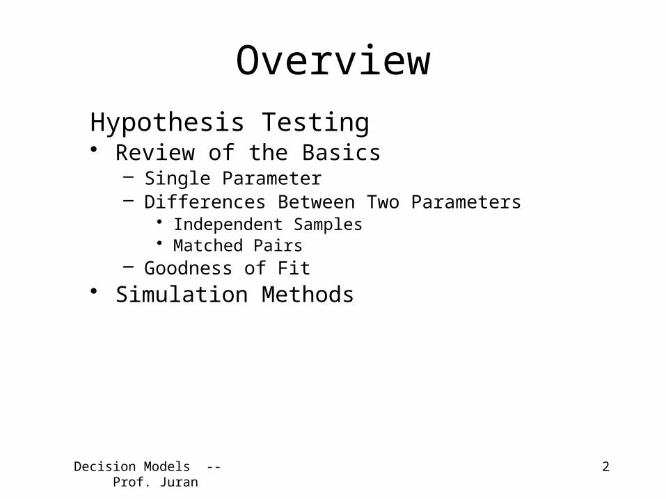
OverviewHypothesis Testing • Review of the Basics
– Single Parameter– Differences Between Two Parameters
• Independent Samples• Matched Pairs
– Goodness of Fit• Simulation Methods

Decision Models -- Prof. Juran
3
Basic Hypothesis Testing Method
1. Formulate Two Hypotheses
2. Select a Test Statistic
3. Derive a Decision Rule
4. Calculate the Value of the Test Statistic; Invoke the Decision Rule in light of the Test Statistic

Decision Models -- Prof. Juran
4
H0 is true HA is true Do Not Reject H0 Correct Decision ERROR (Type II)
Reject H0 ERROR (Type I) Correct Decision
Type I: Reject H0 when H0 is in fact true (reject a true hypothesis).
Type II: Do Not Reject H0 when HA is in fact true ("accept" a false hypothesis).
Let = probability of a Type I Error = P(reject H0 | H0 is true),
= probability of a Type II Error = P("accept" H0 | HA is true).

Applied Regression -- Prof. Juran
5
Hypothesis Testing: Gardening Analogy
Rocks Dirt

Applied Regression -- Prof. Juran
6
Hypothesis Testing: Gardening Analogy

Applied Regression -- Prof. Juran
7
Hypothesis Testing: Gardening Analogy

Applied Regression -- Prof. Juran
8
Hypothesis Testing: Gardening Analogy

Applied Regression -- Prof. Juran
9
Hypothesis Testing: Gardening Analogy
Screened out stuff:Correct decision or Type I
Error?
Stuff that fell through:Correct decision or Type II
Error?
Decision Models -- Prof. Juran
10
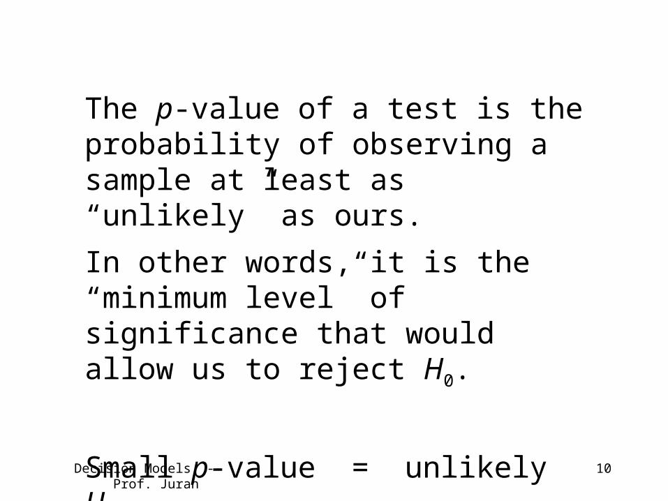
The p-value of a test is the probability of observing a sample at least as “unlikely” as ours.
In other words, it is the “minimum level” of significance that would allow us to reject H0.
Small p-value = unlikely H0

Decision Models -- Prof. Juran
11
Example: Buying a Laundromat
A potential entrepreneur is considering the purchase of a coin-operated laundry. The present owner claims that over the past 5 years the average daily revenue has been $675. The buyer would like to find out if the true average daily revenue is different from $675.
A sample of 30 selected days reveals a daily average revenue of $625 with a standard deviation of $75.

Decision Models -- Prof. Juran
12
H0: 675 HA: 675

Decision Models -- Prof. Juran
13
Test Statistic:
Decision Rule, based on alpha of 1%: Reject H0 if the test statistic is greater than 2.575 or less than -2.575.
ns
Xz 0
0

Decision Models -- Prof. Juran
14
0z ns
X 0
3075
675625
65.3

Decision Models -- Prof. Juran
15
We reject H0. There is sufficiently strong evidence against H0 to reject it at the 0.01 level. We conclude that the true mean is different from $675.

Decision Models -- Prof. Juran
16
Example: Reliability Analysis
123456789
10111213
A B C D E F G H IStart Rank Fail Rank Battery Life Start Time Fail Time
Distribution of battery lifetimes (lognormal) 1 2 Battery A 25.28 0.0 25.3Mean 20 2 1 Battery B 12.02 0.0 12.0Stdev 5 3 3 Battery C 17.00 12.0 29.0
4 5 Battery D 33.15 25.3 58.45 4 Battery E 23.53 29.0 52.5
SimulationFailure# Insert Battery Current time In Position 1 In Position 2
0 Battery A Battery B1 Battery C 12.017 Battery A Battery C 12.022 Battery D 25.275 Battery D Battery C 25.283 Battery E 29.016 Battery D Battery E 29.024 (none) 52.542 Battery D (none) 52.54 <---- Device Fails

Decision Models -- Prof. Juran
17
The brand manager wants to begin advertising for this product, and would like to claim a mean time between failures (MTBF) of 45 hours.
The product is only in the prototype phase, so the design engineer uses Crystal Ball simulation to estimate the product’s reliability characteristics. Extracted data:
1234567891011121314
A BStatistics Fail Time
Trials 1000Mean 43.82Median 43.40Mode ---Standard Deviation 6.09Variance 37.11Skewness 0.47Kurtosis 3.13Coeff. of Variability 0.14Range Minimum 29.12Range Maximum 64.44Range Width 35.32Mean Std. Error 0.19

Decision Models -- Prof. Juran
18
123456789101112131415
A B C D E F GStatistics Fail Time
Trials 1000 Hypothesized MTBF 45Mean 43.82 Test Statistic -6.103Median 43.40 p-ValuesMode --- Upper Tail N/ AStandard Deviation 6.09 Two-Tail 0.0000Variance 37.11 Lower Tail 0.0000Skewness 0.47Kurtosis 3.13Coeff. of Variability 0.14Range Minimum 29.12Range Maximum 64.44Range Width 35.32Mean Std. Error 0.19
=(B3-E2)/(B14)
=IF(E3>0,1-NORMSDIST(E3),"N/A")=(1-NORMSDIST(ABS(E3)))*2=IF(E3<0,NORMSDIST(E3),"N/A")
H0 here is that the product lasts 45 hours (on the average).
There is sufficiently strong evidence against H0 to reject it at any reasonable significance level. We conclude that the true MTBF is less than 45 hours.
Decision Models -- Prof. Juran
19
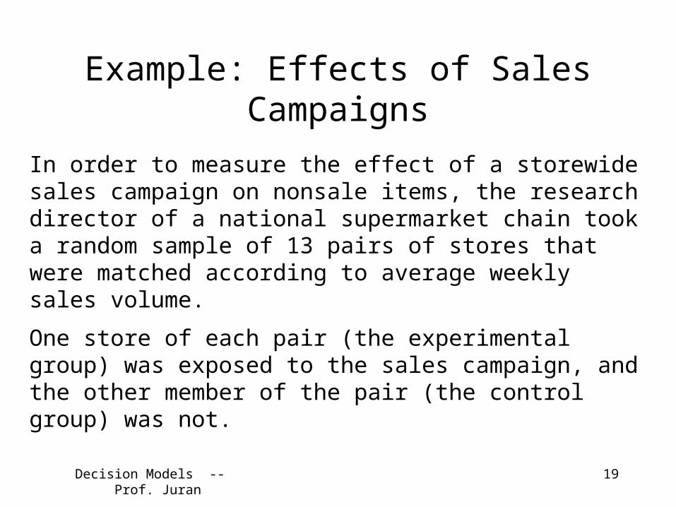
Example: Effects of Sales Campaigns
In order to measure the effect of a storewide sales campaign on nonsale items, the research director of a national supermarket chain took a random sample of 13 pairs of stores that were matched according to average weekly sales volume.
One store of each pair (the experimental group) was exposed to the sales campaign, and the other member of the pair (the control group) was not.

Decision Models -- Prof. Juran
20
The following data indicate the results over a weekly period:
STORE WITH SALES CAMPAIGN WITHOUT SALES CAMPAIGN 1 67.2 65.3 2 59.4 54.7 3 80.1 81.3 4 47.6 39.8 5 97.8 92.5 6 38.4 37.9 7 57.3 52.4 8 75.2 69.9 9 94.7 89.0 10 64.3 58.4 11 31.7 33.0 12 49.3 41.7 13 54.0 53.6

Decision Models -- Prof. Juran
21
Is the campaign effective?
Basically this is asking: Is there a difference between the average sales from these two populations (with and without the campaign)?

Decision Models -- Prof. Juran
22
Two Methods• Independent Samples
– General Method• Matched Pairs
– Useful Only in Specific Circumstances– More Powerful Statistically– Requires Logical One-to-One
Correspondence between Pairs

Decision Models -- Prof. Juran
23
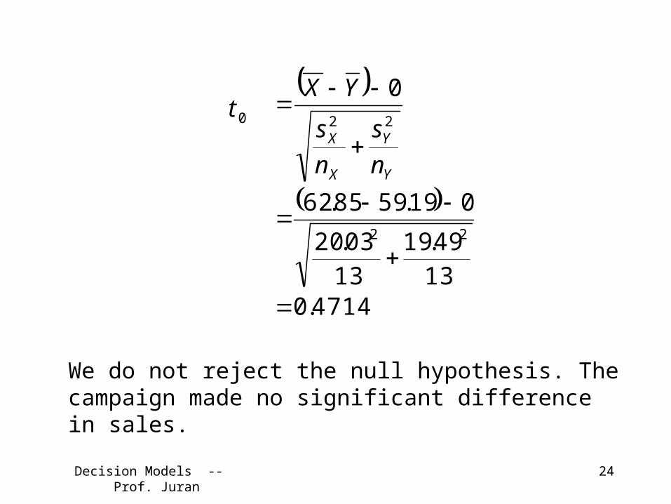
Independent Samples Method
Let the true population mean sales with the campaign be represented by X, and the population mean sales w ithout the campaign be represented by Y .
H 0: 0 YX
H A : 0 YX
We have a small-sample test, so we’ll get our critical value from the t-table. We have one tail, alpha = 0.05, and 12 degrees of freedom, so the critical t-value w ill be 1.782. If the value of our test statistic is greater than 1.782, then we will reject the null hypothesis.
Decision Models -- Prof. Juran
24
0t
Y
Y
X
X
n
s
n
s
YX22
0
13
49.19
13
03.20
019.5985.6222
4714.0
We do not reject the null hypothesis. The campaign made no significant difference in sales.

Decision Models -- Prof. Juran
25
123456789
1011121314
A B C D E F G H I J K
STOREWITH SALES CAMPAIGN
WITHOUT SALES CAMPAIGN
1 67.2 65.3 Sample 1 mean 62.852 59.4 54.7 stdev 20.033 80.1 81.3 n 134 47.6 39.8 Sample 2 mean 59.195 97.8 92.5 stdev 19.496 38.4 37.9 n 137 57.3 52.4 H0 08 75.2 69.99 94.7 89 test stat 0.471410 64.3 58.4 tails 111 31.7 33 p-value 0.322912 49.3 41.713 54 53.6
=AVERAGE($B$2:$B$14)=STDEV($B$2:$B$14)=COUNT($B$2:$B$14)=AVERAGE($C$2:$C$14)=STDEV($C$2:$C$14)=COUNT($C$2:$C$14)
=((G2-G5)-G8)/SQRT(((G3^2)/G4)+((G6^2)/G7))
=TDIST(G10,G4-1,G11)

Decision Models -- Prof. Juran
26
Matched-Pairs Method
Let the true difference between the population means be represented by D. H0: 0D
HA: 0D
The critical t-value will still be 1.782. If the value of our test statistic is greater than 1.782, then we will reject the null hypothesis.

Decision Models -- Prof. Juran
27
0t
n
sD
D
0
13
1855.306538.3
14.4
This time we do reject the null hypothesis, and conclude that the campaign actually did have a significant positive effect on sales.

Decision Models -- Prof. Juran
28
123456789
10111213141516
A B C D E F G H I J K L M
STORE
WITH SALES
CAMPAIGN
WITHOUT SALES CAMPAIGN Difference
1 67.2 65.3 1.90 tails 12 59.4 54.7 4.70 alpha 0.053 80.1 81.3 -1.20 critical t 1.7824 47.6 39.8 7.80 Ho 05 97.8 92.5 5.30 n 136 38.4 37.9 0.50 d-bar 3.65387 57.3 52.4 4.90 stdev 3.18558 75.2 69.9 5.309 94.7 89 5.70 test statistic 4.135610 64.3 58.4 5.90 p-value 0.000711 31.7 33 -1.3012 49.3 41.7 7.6013 54 53.6 0.40
3.653.19
=AVERAGE(D2:D14)=STDEV(D2:D14)
=IF(G2=2,TINV(G3,G6-1),TINV(G3*2,G6-1))
=COUNT(D2:D14)=AVERAGE(D2:D14)=STDEV(D2:D14)
=(G7-G5)/(G8/SQRT(G6))=TDIST(ABS(J10),G6-1,G2)

Decision Models -- Prof. Juran
29
TSB Problem RevisitedTSB Simulation Analysis Results
$32,500
$32,600
$32,700
$32,800
$32,900
$33,000
$33,100
$33,200
$33,300
$33,400
$33,500
$1000 $1250 $1500 $1750 $2000 $2250 $2500 $2750 $3000 $3250
Amount Put Into TSB Account
Me
an
Ne
t In
co
me

Decision Models -- Prof. Juran
30
Independent Samples
123456789
1011121314151617
A B C D E F G H I J KTSB Amount (Decision Variable) 1,000$ 1,250$ 1,500$ 1,750$ 2,000$ 2,250$ 2,500$ 2,750$ 3,000$ 3,250$
Annual Salary 50,000$ 50,000$ 50,000$ 50,000$ 50,000$ 50,000$ 50,000$ 50,000$ 50,000$ 50,000$ Tax Rate 30% 30% 30% 30% 30% 30% 30% 30% 30% 30%After TSB Income 49,000$ 48,750$ 48,500$ 48,250$ 48,000$ 47,750$ 47,500$ 47,250$ 47,000$ 46,750$ Taxes Owed 14,700$ 14,625$ 14,550$ 14,475$ 14,400$ 14,325$ 14,250$ 14,175$ 14,100$ 14,025$ Net Income Before Medical Expenses 34,300$ 34,125$ 33,950$ 33,775$ 33,600$ 33,425$ 33,250$ 33,075$ 32,900$ 32,725$
Total Medical Expenses 2,675.05$ Amount in TSB 1,000.00$ 1,250.00$ 1,500.00$ 1,750.00$ 2,000.00$ 2,250.00$ 2,500.00$ 2,750.00$ 3,000.00$ 3,250.00$ Expenses Not Covered (Must Be Paid Out-Of-Pocket) 1,675.05$ 1,425.05$ 1,175.05$ 925.05$ 675.05$ 425.05$ 175.05$ -$ -$ -$ Money Left Over in TSB (Lost) -$ -$ -$ -$ -$ -$ -$ 74.95$ 324.95$ 574.95$
Net Income After Medical Expenses (Objective) 32,624.95$ 32,699.95$ 32,774.95$ 32,849.95$ 32,924.95$ 32,999.95$ 33,074.95$ 33,075.00$ 32,900.00$ 32,725.00$
Mean 2,000.00$ Standard Deviation 500.00$

Decision Models -- Prof. Juran
31
1234567891011121314
A B C D E F G H I J KStatistics $1000 $1250 $1500 $1750 $2000 $2250 $2500 $2750 $3000 $3250
Trials 10000 10000 10000 10000 10000 10000 10000 10000 10000 10000Mean $33,298.70 $33,362.99 $33,409.96 $33,427.00 $33,401.28 $33,326.98 $33,209.51 $33,061.48 $32,895.94 $32,723.82 Median $33,302.16 $33,377.16 $33,452.16 $33,527.16 $33,600.00 $33,425.00 $33,250.00 $33,075.00 $32,900.00 $32,725.00 Mode $34,300.00 $34,125.00 $33,950.00 $33,775.00 $33,600.00 $33,425.00 $33,250.00 $33,075.00 $32,900.00 $32,725.00 Standard Deviation $490.65 $471.50 $432.23 $369.89 $289.49 $203.64 $128.08 $73.17 $39.85 $20.85 Variance $240,739.17 $222,316.85 $186,824.96 $136,817.78 $83,805.39 $41,470.22 $16,404.53 $5,353.44 $1,587.82 $434.85 Skewness -0.11 -0.28 -0.57 -1.01 -1.64 -2.64 -4.39 -7.81 -13.77 -23.28Kurtosis 2.75 2.64 2.77 3.51 5.58 11.08 27.13 79.33 232.03 623.10Coeff. of Variability 0.01 0.01 0.01 0.01 0.01 0.01 0.00 0.00 0.00 0.00Minimum $31,268.67 $31,343.67 $31,418.67 $31,493.67 $31,568.67 $31,643.67 $31,718.67 $31,793.67 $31,868.67 $31,943.67 Maximum $34,300.00 $34,125.00 $33,950.00 $33,775.00 $33,600.00 $33,425.00 $33,250.00 $33,075.00 $32,900.00 $32,725.00 Range Width $3,031.33 $2,781.33 $2,531.33 $2,281.33 $2,031.33 $1,781.33 $1,531.33 $1,281.33 $1,031.33 $781.33 Mean Std. Error $4.91 $4.72 $4.32 $3.70 $2.89 $2.04 $1.28 $0.73 $0.40 $0.21
Decision Models -- Prof. Juran
32
123456789
10111213141516171819
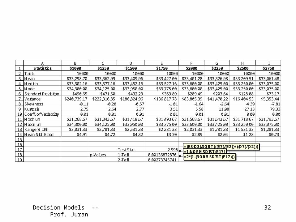
A B C D E F G H IStatistics $1000 $1250 $1500 $1750 $2000 $2250 $2500 $2750
Trials 10000 10000 10000 10000 10000 10000 10000 10000Mean $33,298.70 $33,362.99 $33,409.96 $33,427.00 $33,401.28 $33,326.98 $33,209.51 $33,061.48 Median $33,302.16 $33,377.16 $33,452.16 $33,527.16 $33,600.00 $33,425.00 $33,250.00 $33,075.00 Mode $34,300.00 $34,125.00 $33,950.00 $33,775.00 $33,600.00 $33,425.00 $33,250.00 $33,075.00 Standard Deviation $490.65 $471.50 $432.23 $369.89 $289.49 $203.64 $128.08 $73.17 Variance $240,739.17 $222,316.85 $186,824.96 $136,817.78 $83,805.39 $41,470.22 $16,404.53 $5,353.44 Skewness -0.11 -0.28 -0.57 -1.01 -1.64 -2.64 -4.39 -7.81Kurtosis 2.75 2.64 2.77 3.51 5.58 11.08 27.13 79.33Coeff. of Variability 0.01 0.01 0.01 0.01 0.01 0.01 0.00 0.00Minimum $31,268.67 $31,343.67 $31,418.67 $31,493.67 $31,568.67 $31,643.67 $31,718.67 $31,793.67 Maximum $34,300.00 $34,125.00 $33,950.00 $33,775.00 $33,600.00 $33,425.00 $33,250.00 $33,075.00 Range Width $3,031.33 $2,781.33 $2,531.33 $2,281.33 $2,031.33 $1,781.33 $1,531.33 $1,281.33 Mean Std. Error $4.91 $4.72 $4.32 $3.70 $2.89 $2.04 $1.28 $0.73
Test Stat 2.996p-Values 1-Tail 0.00136872870
2-Tail 0.00273745741
=(E3-D3)/SQRT(((E7)/(E2))+((D7)/(D2)))=1-NORMSDIST(E17)=2*(1-(NORMSDIST(E17)))

Decision Models -- Prof. Juran
33
Matched Pairs
123456789
1011121314151617181920
A B C D E FTSB Amount (Decision Variable) 1,000$ 1,250$ 1,500$ 1,750$ 2,000$
Annual Salary 50,000$ 50,000$ 50,000$ 50,000$ 50,000$ Tax Rate 30% 30% 30% 30% 30%After TSB Income 49,000$ 48,750$ 48,500$ 48,250$ 48,000$ Taxes Owed 14,700$ 14,625$ 14,550$ 14,475$ 14,400$ Net Income Before Medical Expenses 34,300$ 34,125$ 33,950$ 33,775$ 33,600$
Total Medical Expenses 2,675.05$ Amount in TSB 1,000.00$ 1,250.00$ 1,500.00$ 1,750.00$ 2,000.00$ Expenses Not Covered (Must Be Paid Out-Of-Pocket) 1,675.05$ 1,425.05$ 1,175.05$ 925.05$ 675.05$ Money Left Over in TSB (Lost) -$ -$ -$ -$ -$
Net Income After Medical Expenses (Objective) 32,624.95$ 32,699.95$ 32,774.95$ 32,849.95$ 32,924.95$
Mean 2,000.00$ Standard Deviation 500.00$
Difference 75.00$ (1750 vs 1500)
=E14-D14
Decision Models -- Prof. Juran
34

Decision Models -- Prof. Juran
35
12345678910111213141516171819
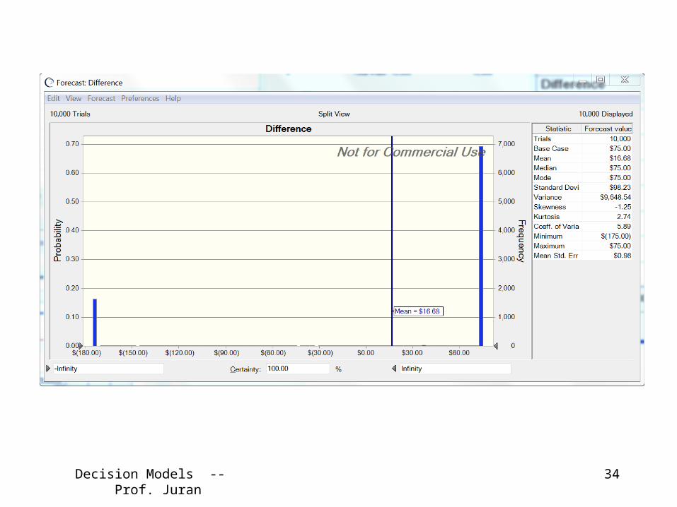
A B C D E F GStatistics $1500 $1750 Difference
Trials 10000 10000 10000Base Case $32,774.95 $32,849.95 $75.00Mean $33,408.09 $33,426.42 $16.68Median $33,447.04 $33,522.04 $75.00Mode $33,950.00 $33,775.00 $75.00Standard Deviation $432.25 $371.37 $98.23Variance $186,836.67 $137,917.72 $9,648.54Skewness -0.5887 -1.02 -1.25Kurtosis 2.78 3.49 2.74Coeff. of Variation 0.0129 0.0111 5.89Minimum $31,506.74 $31,581.74 $(175.00)Maximum $33,950.00 $33,775.00 $75.00Range Width $2,443.26 $2,193.26 $250.00Mean Std. Error $4.32 $3.71 $0.98
Test Stat 16.978056970.00000000.0000000
=D4/D15=1-NORMSDIST(D17)=2*(1-NORMSDIST(D17))
Decision Models -- Prof. Juran
36
Goodness-of-Fit Tests
• Determine whether a set of sample data have been drawn from a hypothetical population
• Same four basic steps as other hypothesis tests we have learned
• An important tool for simulation modeling; used in defining random variable inputs

37
Example: Barkevious Mingo
Financial analyst Barkevious Mingo wants to run a simulation model that includes the assumption that the daily volume of a specific type of futures contract traded at U.S. commodities exchanges (represented by the random variable X) is normally distributed with a mean of 152 million contracts and a standard deviation of 32 million contracts. (This assumption is based on the conclusion of a study conducted in 2013.) Barkevious wants to determine whether this assumption is still valid.
Decision Models -- Prof. Juran

38
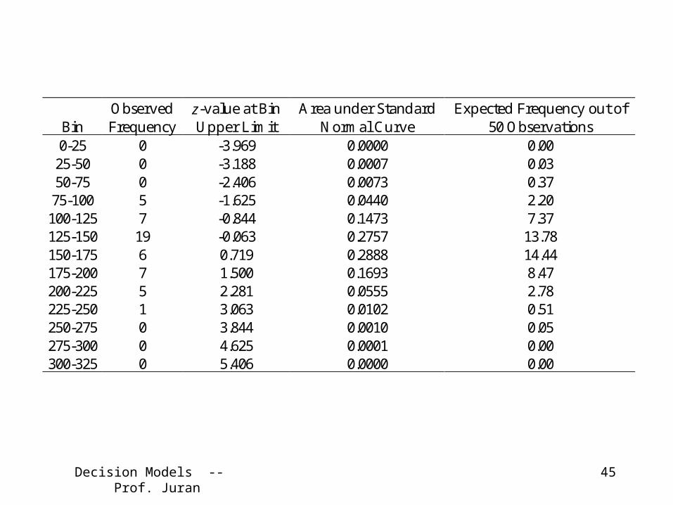
He studies the trading volume of these contracts for 50 days, and observes the following results (in millions of contracts traded):
142.4 207.5 129.9 84.2 149.3 105.8 152.9 141.5 135.6 205.2 111.1 82.1 97.9 133.8 135.2 124.9 141.7 140.2 215.1 100.4 159.8 144.5 92.9 139.1 173.6 103.3 222.2 195.0 179.7 169.2 192.8 187.0 120.7 156.3 139.8 140.4 96.2 149.3 228.0 180.9 190.3 117.2 127.2 140.3 176.2 151.0 128.4 146.0 131.0 213.4
Decision Models -- Prof. Juran

39
Bin Observed Frequency
z-value at Bin Upper Limit
Area under Standard Normal Curve
Expected Frequency out of 50 Observations
0-25 0 -3.969 0.0000 0.00 25-50 0 -3.188 0.0007 0.03 50-75 0 -2.406 0.0073 0.37 75-100 5 -1.625 0.0440 2.20 100-125 7 -0.844 0.1473 7.37 125-150 19 -0.063 0.2757 13.78 150-175 6 0.719 0.2888 14.44 175-200 7 1.500 0.1693 8.47 200-225 5 2.281 0.0555 2.78 225-250 1 3.063 0.0102 0.51 250-275 0 3.844 0.0010 0.05 275-300 0 4.625 0.0001 0.00 300-325 0 5.406 0.0000 0.00
Decision Models -- Prof. Juran

40
Here is a histogram showing the theoretical distribution of 50 observations drawn from a normal distribution with μ = 152 and σ = 32, together with a histogram of Mingo’s sample data:
"Eyeball" Hypothesis Test: Expected Distribution
0
5
10
15
20
0-25 25-50 50-75 75-100 100-125 125-150 150-175 175-200 200-225 225-250 250-275 275-300 300-325
Number of Contracts Traded
Fr
eq
ue
nc
y
"Eyeball" Hypothesis Test: Observed Distribution
0
5
10
15
20
0-25 25-50 50-75 75-100 100-125 125-150 150-175 175-200 200-225 225-250 250-275 275-300 300-325
Number of Contracts Traded
Fr
eq
ue
nc
y
Decision Models -- Prof. Juran

41
2
e
eo
f
ff 2
of = the observed frequency of data in a specific range
ef = the expected frequency of data in a specific range
The Chi-Square Statistic
Decision Models -- Prof. Juran
42
Essentially, this statistic allows us to compare the distribution of a sample with some expected distribution, in standardized terms. It is a measure of how much a sample differs from some proposed distribution.
A large value of chi-square suggests that the two distributions are not very similar; a small value suggests that they “fit” each other quite well.
Decision Models -- Prof. Juran

43
Like Student’s t, the distribution of chi-square depends on degrees of freedom.
In the case of chi-square, the number of degrees of freedom is equal to the number of classes (a.k.a. “bins” into which the data have been grouped) minus one, minus the number of estimated parameters.
Decision Models -- Prof. Juran

44
H ere are grap h s sh ow in g th e ch i -sq u are d istrib u tion for sev eral d iff eren t n u m b ers of d egrees of f reed om :
0 .0 0 0
0 .0 0 5
0 .0 1 0
0 .0 1 5
0 .0 2 0
0 5 1 0 1 5 2 0 2 5 3 0 3 5 4 0 4 5 5 0
C h i - S q u a r e S t a t i s t i c
Proba
bility
0 .0 0 0
0 .0 0 5
0 .0 1 0
0 .0 1 5
0 .0 2 0
0 5 1 0 1 5 2 0 2 5 3 0 3 5 4 0 4 5 5 0
C h i - S q u a r e S t a t i s t i c
Proba
bility
C h i -S q u are D i strib u tion , d.f. = 5 C h i -S q u are D i strib u tion , d.f. = 10
0 .0 0 0
0 .0 0 5
0 .0 1 0
0 .0 1 5
0 .0 2 0
0 5 1 0 1 5 2 0 2 5 3 0 3 5 4 0 4 5 5 0
C h i - S q u a r e S t a t i s t i c
Proba
bility
0 .0 0 0
0 .0 0 5
0 .0 1 0
0 .0 1 5
0 .0 2 0
0 5 1 0 1 5 2 0 2 5 3 0 3 5 4 0 4 5 5 0
C h i - S q u a r e S t a t i s t i c
Proba
bility
C h i -S q u are D i strib u tion , d.f. = 15 C h i -S q u are D i strib u tion , d.f. = 20
Decision Models -- Prof. Juran
45
Bin Observed Frequency
z-value at Bin Upper Limit
Area under Standard Normal Curve
Expected Frequency out of 50 Observations
0-25 0 -3.969 0.0000 0.00 25-50 0 -3.188 0.0007 0.03 50-75 0 -2.406 0.0073 0.37 75-100 5 -1.625 0.0440 2.20 100-125 7 -0.844 0.1473 7.37 125-150 19 -0.063 0.2757 13.78 150-175 6 0.719 0.2888 14.44 175-200 7 1.500 0.1693 8.47 200-225 5 2.281 0.0555 2.78 225-250 1 3.063 0.0102 0.51 250-275 0 3.844 0.0010 0.05 275-300 0 4.625 0.0001 0.00 300-325 0 5.406 0.0000 0.00
Decision Models -- Prof. Juran

46
Note: It is necessary to have a sufficiently large sample so that each class has an expected frequency of at least 5. We need to make sure that the expected frequency in each bin is at least 5, so we “collapse” some of the bins, as shown here.
Bin Observed Frequency
z-value at Bin Upper
Limit
Area under Standard
Normal Curve
Expected Frequency out of 50
Observations 0-125 12 -0.844 0.1994 9.97
125-150 19 -0.063 0.2757 13.78 150-175 6 0.719 0.2888 14.44 175-325 13 5.406 0.2361 11.81
Decision Models -- Prof. Juran
47
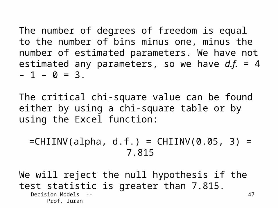
The number of degrees of freedom is equal to the number of bins minus one, minus the number of estimated parameters. We have not estimated any parameters, so we have d.f. = 4 – 1 – 0 = 3.
The critical chi-square value can be found either by using a chi-square table or by using the Excel function:
=CHIINV(alpha, d.f.) = CHIINV(0.05, 3) = 7.815
We will reject the null hypothesis if the test statistic is greater than 7.815.
Decision Models -- Prof. Juran

48
Bin Observed Frequency Expected Frequency out of 50 Observations e
eo
f
ff 2
0-125 12 9.97 0.413 125-150 19 13.78 1.974 150-175 6 14.44 4.932 175-325 13 11.81 0.120 Chi-Square = 7.439
Our test statistic is not greater than the critical value; we cannot reject the null hypothesis at the 0.05 level of significance.
It would appear that Barkevious is justified in using the normal distribution with μ = 152 and σ = 32 to model futures contract trading volume in his simulation.
Decision Models -- Prof. Juran
49
0.000
0.005
0.010
0.015
0.020
0.025
0.030
0 2 4 6 8 10 12 14 16 18 20
Critical Value of Chi-Square = 7.815Test Statistic = 7.439
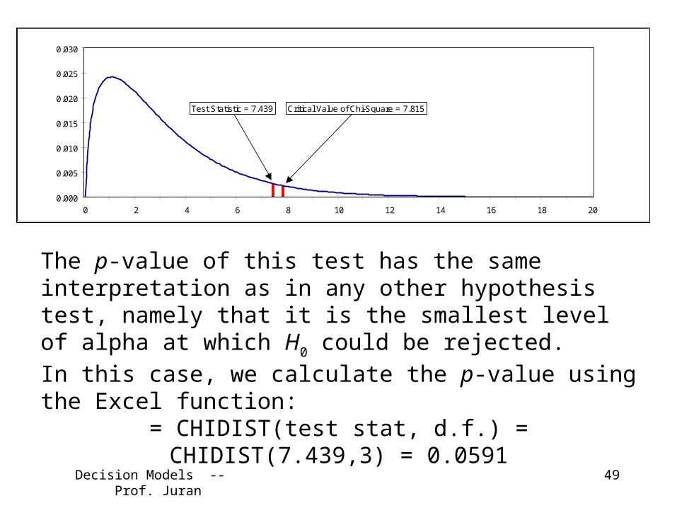
The p-value of this test has the same interpretation as in any other hypothesis test, namely that it is the smallest level of alpha at which H0 could be rejected. In this case, we calculate the p-value using the Excel function:
= CHIDIST(test stat, d.f.) = CHIDIST(7.439,3) = 0.0591
Decision Models -- Prof. Juran

50
Example: Catalog Company
If we want to simulate the queueing system at this company, what distributions should we use for the arrival and service processes?
Decision Models -- Prof. Juran
51
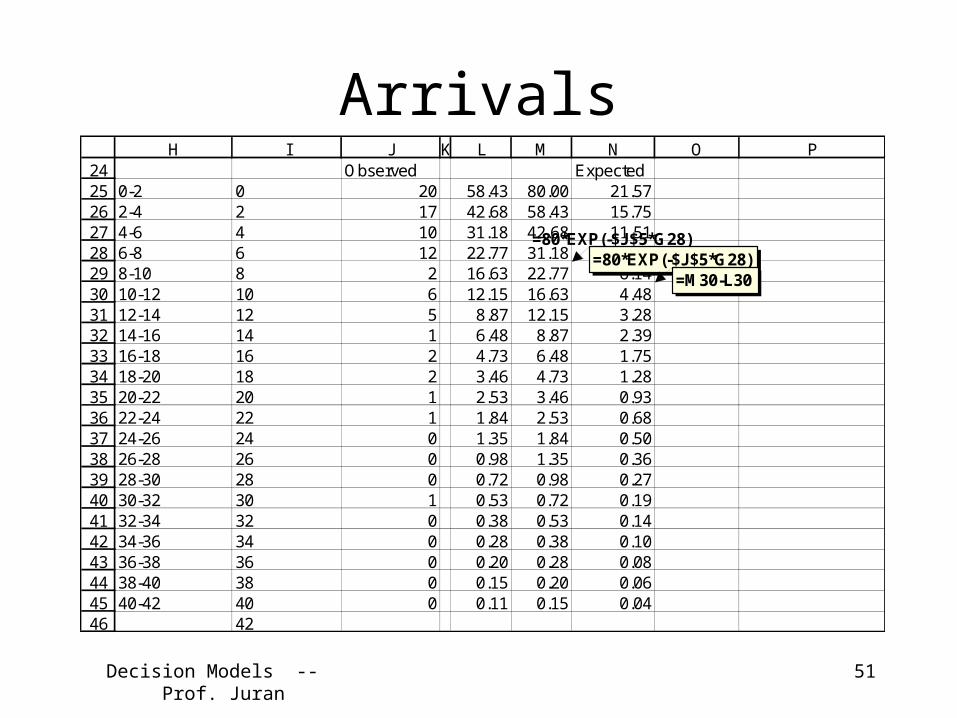
Arrivals2425262728293031323334353637383940414243444546
H I J K L M N O PObserved Expected
0-2 0 20 58.43 80.00 21.572-4 2 17 42.68 58.43 15.754-6 4 10 31.18 42.68 11.516-8 6 12 22.77 31.18 8.408-10 8 2 16.63 22.77 6.1410-12 10 6 12.15 16.63 4.4812-14 12 5 8.87 12.15 3.2814-16 14 1 6.48 8.87 2.3916-18 16 2 4.73 6.48 1.7518-20 18 2 3.46 4.73 1.2820-22 20 1 2.53 3.46 0.9322-24 22 1 1.84 2.53 0.6824-26 24 0 1.35 1.84 0.5026-28 26 0 0.98 1.35 0.3628-30 28 0 0.72 0.98 0.2730-32 30 1 0.53 0.72 0.1932-34 32 0 0.38 0.53 0.1434-36 34 0 0.28 0.38 0.1036-38 36 0 0.20 0.28 0.0838-40 38 0 0.15 0.20 0.0640-42 40 0 0.11 0.15 0.04
42
=80*EXP(-$J$5*G28)=80*EXP(-$J$5*G28)
=M30-L30
Decision Models -- Prof. Juran
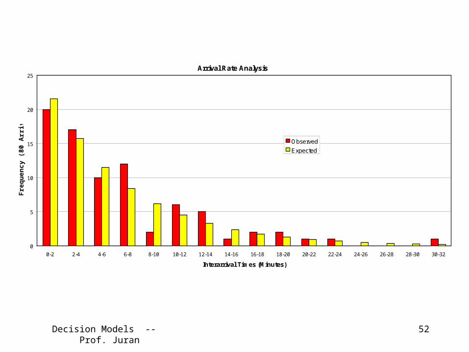
52
Arrival Rate Analysis
0
5
10
15
20
25
0-2 2-4 4-6 6-8 8-10 10-12 12-14 14-16 16-18 18-20 20-22 22-24 24-26 26-28 28-30 30-32
Interarrival Times (Minutes)
Fre
qu
ency
(80
Arr
ival
s)
Observed
Expected
Decision Models -- Prof. Juran

53
25262728293031323334
Q R S T U V W X Y ZObserved Expected
0-2 20 58.43374 80 21.56626 0.1137512-4 17 42.68127 58.43374 15.75247 0.09884-6 10 31.17533 42.68127 11.50594 0.1971046-8 12 22.77113 31.17533 8.404191 1.5384998-10 2 16.63253 22.77113 6.138604 2.79021810-14 11 12.14876 16.63253 7.758812 1.35398314-32 8 6.481557 8.873719 8.76454 0.066692
6.159046
=(R26-V26)^2/V26
=SUM(W26:W32)
Decision Models -- Prof. Juran

54
2526272829303132333435363738
Q R S T U V WObserved Expected
0-2 20 58.43374 80 21.56626 0.1137512-4 17 42.68127 58.43374 15.75247 0.09884-6 10 31.17533 42.68127 11.50594 0.1971046-8 12 22.77113 31.17533 8.404191 1.5384998-10 2 16.63253 22.77113 6.138604 2.79021810-14 11 12.14876 16.63253 7.758812 1.35398314-32 8 6.481557 8.873719 8.76454 0.066692
6.159046d.f. 6alpha 0.05critical value 12.5916test stat 6.1590p-value 0.4056
=CHIINV(S35,S34)=W33=CHIDIST(S37,S34)
Decision Models -- Prof. Juran

55
Goodness of Fit Test for Arrivals
0.0000
0.0020
0.0040
0.0060
0.0080
0.0100
0.0120
0.0140
0.0160
0 2 4 6 8 10 12 14 16 18 20 22 24 26 28 30 32 34 36 38 40 42 44 46 48 50
Chi Square
Pro
bab
ilit
y
Test Statistic = 6.159
Critical Value = 12.59
Area Under the Curve > 6.159 = 0.4056
Decision Models -- Prof. Juran

56
ServicesService Rate Analysis
0
2
4
6
8
10
12
14
16
18
0-2 2-4 4-6 6-8 8-10 10-12 12-14 14-16 16-18 18-20 20-22 22-24 24-26 26-28 28-30 30-32 32-34 34-36 36-38 38-40 40-42
Interarrival Times (Minutes)
Fre
qu
ency
(80
Arr
ival
s)
Observed
Expected
Decision Models -- Prof. Juran

57
Goodness of Fit Test for Services
0.0000
0.0020
0.0040
0.0060
0.0080
0.0100
0.0120
0.0140
0.0160
0 2 4 6 8 10 12 14 16 18 20 22 24 26 28 30 32 34 36 38 40 42 44 46 48 50
Chi Square
Pro
bab
ilit
y
Test Statistic = 47.79
Critical Value = 11.07
Area Under the Curve > 47.79 = 0.0000
Decision Models -- Prof. Juran

142.4 207.5 129.9 84.2 149.3 105.8 152.9 141.5 135.6 205.2
111.1 82.1 97.9 133.8 135.2 124.9 141.7 140.2 215.1 100.4
159.8 144.5 92.9 139.1 173.6 103.3 222.2 195.0 179.7 169.2
192.8 187.0 120.7 156.3 139.8 140.4 96.2 149.3 228.0 180.9
190.3 117.2 127.2 140.3 176.2 151.0 128.4 146.0 131.0 213.4
Decision Models -- Prof. Juran
Decision Models -- Prof. Juran
59

Decision Models -- Prof. Juran
60
Decision Models -- Prof. Juran
61

Decision Models -- Prof. Juran
62
1
2
3
4
5
6
7
8
9
A B C D
142.4
111.1
159.8
192.8
190.3 0
207.5
82.1
144.5
187.0

63
Other uses for the Chi-Square statistic
• Tests of the independence of two qualitative population variables.
• Tests of the equality or inequality of more than two population proportions.
• Inferences about a population variance, including the estimation of a confidence interval for a population variance from sample data.
The chi-square technique can often be employed for purposes of estimation or hypothesis testing when the z or t statistics are not appropriate. In addition to the goodness-of-fit application described above, there are at least three other important uses for chi-square:
Decision Models -- Prof. Juran

Decision Models -- Prof. Juran
64
SummaryHypothesis Testing • Review of the Basics
– Single Parameter– Differences Between Two Parameters
• Independent Samples• Matched Pairs
– Goodness of Fit• Simulation Methods