service capacity decision and incentive compatible cost allocation for reporting usage forecasts

European Journal of Operational Research 157 (2004) 180–195

www.elsevier.com/locate/dsw

Stochastics and Statistics

Service capacity decision and incentive compatiblecost allocation for reporting usage forecasts

Suresh Radhakrishnan a,*, Kashi R. Balachandran b

a School of Management, University of Texas at Dallas, Mail Stop JO43, Richardson, TX 75083, USAb Stern School of Business, New York University, NY 10012, USA

Received 16 May 2002; accepted 18 March 2003

Abstract

We consider anM/G/1 queue with multiple users where service capacity can be improved at a cost by reducing the mean

and variance of service time and each user has private information on his expected usage. The firm�s headquarter requiresinformation on expected usage to determine the optimum service capacity. We develop a simple cost allocation scheme

where a charge is applied to realized usage. This charge is computed by dividing the service capacity costs by the total

reported expected usage weighted by the cost per unit time delay. The difference between the service capacity cost and the

total charge applied to realized usage is credited/charged to the users based on the proportion of reported expected usage

weighted by the cost per unit time delay. This cost allocation scheme (a) induces truthful reports of expected usage, (b)

maximizes the expected net benefit of each user with respect to the service capacity, (c) shares all the service capacity costs,

(d) achieves the same service capacity that the firm�s headquarter would choose in an unconstrained maximization

problem with no private information, and (e) uses only the realized and reported expected usages. We also examine

whether the cost allocation scheme provides incentives for each user to obtain good forecasts on expected usage.

� 2003 Elsevier B.V. All right reserved.

Keywords: Game theory; Mechanism design; Truth-telling; Queues; Delay cost; Congestion

1. Introduction

We examine an incentive problem associated with obtaining information on expected usage from theusers for determining service capacity improvements. The firm�s headquarters faces two important decisions

with respect to the service center. First, the firm�s headquarter needs to regulate the relative usage of the

service center for a given service capacity. For this purpose adequate incentives need to be provided to the

users for inducing the optimum usage. 1 Second, the firm�s headquarter has to decide the service capacity

* Corresponding author. Tel.: +1-972-8834438; fax: +1-972-8836811.

E-mail address: [email protected] (S. Radhakrishnan).1 A number of papers have examined the issue of regulating usage. Balachandran and Schaefer (1979, 1980), Balachandran and

Radhakrishnan (1994), Mendelson and Whang (1990, 1994) and Radhakrishnan and Balachandran (1995) analyze conflicts between

social and private optimum usage, and provide insights into optimal admission policies and pricing schemes.

0377-2217/$ - see front matter � 2003 Elsevier B.V. All right reserved.

doi:10.1016/S0377-2217(03)00246-7

mail to: [email protected]

S. Radhakrishnan, K.R. Balachandran / European Journal of Operational Research 157 (2004) 180–195 181

based on the requirements of the users. For this purpose incentives need to be provided to the users suchthat information on forecasted usage is reported truthfully.

In this paper, we examine the service capacity improvement decision when users have private infor-

mation on expected usage. The service center is shared by various products (departments) with a product

(department) manager in-charge, i.e., user, who is interested in maximizing his profit. We model the service

center as a first-come-first-serve M/G/1 queue. The demands for each user i arise from a Poisson process

with arrival rate ki and the expected benefit per use is gi. The expected waiting time for each use is Wi and

the cost per unit of wait is vi. During the budgeting cycle, each user forecasts his expected usage and reports

it to the headquarter. These demand forecasts are used to determine the level of service capacity im-provements at a cost C. The service capacity improvement is achieved by reducing the mean service time

and/or the variance of service time. Each user is allocated ai proportion of the cost C, and each user�sexpected net benefit is Bi ¼ ki½gi � viWi � � aiC. This model extends the information technology setting

considered in Mendelson and Whang (1990) by introducing the service center capacity decision when users

have private information on expected usage. The forecasts of expected usage are important inputs for

planning medium-run service capacity. Accurate allocation of service capacity cost is important for product

decisions such as the product add/drop decision, the product pricing decision and the outsourcing decision.

This is especially the case for service capacity decisions that result in intangible benefits such as decreasedwaiting costs. The managerial question that we address is what is the appropriate cost driver that should be

used to allocate service improvement costs accurately to products such that the service capacity decision is

not distorted. Furthermore, the cost allocation scheme should also provide an incentive for the product

managers to report their forecasts truthfully.

We develop a simple cost allocation scheme that works as follows. For each realized a charge per use

weighted by the cost per unit time delay is applied. This charge per use is the service capacity cost divided by

the total reported expected usage weighted by the cost per unit time delay (average cost per use), which is

similar to the standard cost per use. Since, the realized use is a random variable, the total charge applied toall users could be either higher or lower than the service capacity cost. This over-/under-charge is credited/

charged to the users in the proportion of the reported expected usage weighted by the cost per unit time

delay.

The cost allocation scheme is simple to implement and has many desirable properties. First, the cost

allocation scheme distributes the capacity cost among all users. Second, the cost allocation scheme maxi-

mizes the expected net benefit of each user with respect to the optimum service capacity, i.e., the scheme is

incentive compatible with respect to service capacity. Third, the cost allocation scheme uses information on

budgeted and actual usage, and does not require information on delay or service time, making it simple toimplement. Fourth, the cost allocation scheme achieves the same service capacity as the firm would choose

in an unconstrained maximization problem with no private information, i.e., the scheme achieves the first-

best efficient capacity. Finally, the cost allocation scheme is similar to the budgeted-cost allocation scheme

described in management accounting texts (see Horngren et al., 2000) with the addition of disposing the

under-/over-charge to the users. Thus, the proposed cost allocation scheme does not impose additional

complexity on the accounting system.

The important managerial insight provided by the analysis is that volume-based cost drivers are suffi-

cient to induce first-best efficient mean/variance of service time improvements and obtain good usageforecasts. This is consistent with the empirical finding of Foster and Gupta (1990) who show that over-

head costs are associated with volume-based drivers alone for an electronic component manufacturer.

In effect, measures of waiting and cycle times are not essential for inducing optimal capacity and usage

decisions. That is, the average capacity cost per use of the facility which is a widely used allocation scheme

in practice is sufficient to proxy for negative externality effects and induce truthful reports in the pres-

ence of hidden-information. Another implication of this result is that the normal or expected usage

(activity) level is an appropriate basis for determining the average costs instead of the theoretical usage

182 S. Radhakrishnan, K.R. Balachandran / European Journal of Operational Research 157 (2004) 180–195

(activity) level. 2 Overall, even though the relationship between service capacity and usage is non-linear,a cost allocation scheme based on average costs per use has desirable properties and induces truthful

reports.

A number of studies have examined dominant strategy mechanisms in a scenario where the capacity of a

common facility needs to be determined (see for example, Ronen and McKinney, 1970; Groves and Loeb,

1979; Holmstrom, 1979; Laffont and Maskin, 1980; Walker, 1980; Groves and Ledyard, 1980; Ronen,

1992). They show that any dominant strategy mechanism that is socially optimal belongs to the Groves–

Vickery–Clarke class of mechanisms. These studies considered situations where the realized usage is not

observable and their cost sharing rules use the reported expected usage alone to induce truthful reports.Consequently, in general, the Groves� class of cost allocation schemes do not share all the capacity (see

Laffont and Maskin, 1980). The scheme developed in this paper, distributes all the cost for any realization

of usage––the full costing feature. This property is extremely important for other decisions such as product

pricing at the departmental level, which could get distorted if the cost allocation is greater than or lesser

than the actual cost that the firm incurs (see Horngren et al., 2000).

Miller and Buckman (1987) consider an M/M/s/s queue and examine the role of cost allocation and

service capacity, i.e., the number of service channels. They show that full cost allocation schemes are op-

timal only when the cost of providing service is linear. We extend this by considering (a) non-linear capacitycosts with both fixed and variable components, and (b) forecasting (budgeting) usage, which requires a cost

allocation scheme to elicit the forecasted usage truthfully. Whang (1989) examines a setting where the

optimum capacity of the common facility is determined based on reported usage, where the users know

their usage perfectly and the capacity costs are linear. In contrast, we examine a setting where each user

knows his usage imperfectly (i.e., a forecast of usage) and allow for non-linear capacity costs.

Radhakrishnan and Balachandran (1996) consider an M/M/1 queue and examine the capacity choice

problem when the cost per unit time delay is not known and show that a noisy measure of the cost is

sufficient to achieve the first-best capacity choice. They do not consider the user�s superior informationrelated to expected usage, and thus, no implications are drawn on volume-based cost allocation schemes

and the budgeting process. We extend this by considering an M/G/1 queue to examine the service capacity

improvement decision based on forecasted usage information from the users, which captures the budgeting

process in an organization. The forecasted usage information is not perfect in the sense that the actual

usage could be different from the forecasted usage. We demonstrate an intuitive role for obtaining budgeted

volume (expected usage) reports from managers. Furthermore, the cost allocation scheme that we develop

is similar to cost allocation schemes advocated in managerial accounting texts using volume (usage) based

measures. We also discuss how incentives for obtaining better forecasts can be provided.The rest of the paper is organized as follows: Section 2 considers the benchmark case where all users and

the facility manager know the forecasted usage perfectly; Section 3 analyzes the case where each user knows

his own forecasted usage and has the potential of misreporting the forecasted usage; Section 4 provides a

numerical example and a discussion on forecast errors; and Section 5 contains concluding remarks.

2. Benchmark settings

In this section, we examine two benchmark cases which will help us derive the cost allocation scheme in

the next section.

2 Barefield et al. (1994) state that ‘‘From a long-run perspective, we believe that the costs generated from use of a theoretical

capacity are more reflective of the company�s true costs.’’


2.1. The first-best solution

Consider a service center with n users (products) where the service center capacity is to be determined.

The demand for service follows a Poisson process where the arrival rate (expected usage) for user (product)

i is given by ki. The demands are serviced on a first-come-first-serve basis. The service time for each demand

has a general distribution, with mean ðs� kÞ and variance r2. We let p ¼ 1=r2 and refer to fp; kg as the

measure of service capacity. 3 The total number of service hours available is denoted by T and is kept fixed.

Our focus is on service capacity improvement efforts that include tangible and intangible activities such asworker training, installing modern technologies, streamlining procedures through re-engineering efforts all

of which can decrease the mean service time and/or decrease the variance in service time. The average delay

(total expected waiting time, W ) experienced by any user is given as (see Cooper, 1981)

3 W

with fcapaci

quality4 Th

where

the wo

and ca

cost eq

time d5 Th

quasic6 Of

W ðk; p; kÞ ¼ ðs½ � kÞ þP

j kj

2p½T �P

j kjðs� kÞ� þP

j kjðs� kÞ2

2½T �P

j kjðs� kÞ�

#; ð1Þ

where k ¼ fki : 8ig. Users incur an average cost of vi per unit time delay. The expected benefit for each use

for user i is denoted gi.4

The cost of service capacity per unit time is given by Cðp; kÞ ¼ F þ cðp; kÞ, where F is a fixed cost that

represents the scale of the service center. We assume that oC=op > 0, o2C=op2 > 0, oC=ok > 0, o2C=ok2 > 0and o2C=opok ¼ 0, i.e., the cost of improving the service capacity increases at an increasing rate. 5 We also

assume that limp!0 Cðp; k ¼ 0Þ ¼ 0, which implies that having a service capacity of zero is costless. Also, we

assume that limp!1 Cðp; kÞ ! 1, limk!s Cðp; kÞ ! 1, limp!1 oC=op½ � ! 1, and limk!s oC=ok½ � ! 1.

These assumptions are sufficient to ensure that the optimum service capacity satisfies 1 > p > 0 and

s > kP 0. The headquarter�s total expected net benefit per unit time is 6

Bðk; p; kÞ ¼Xi

kifgi � viW ðk; p; kÞg � Cðp; kÞ: ð2Þ

The problem for the headquarter is given in Program 0.

Program 0

maxp;k

Bðk; p; kÞ: ð3Þ

Program 0 provides the benchmark optimum service capacity that maximizes the headquarter�s total

expected net benefit. The optimum service capacity satisfies the following first-order conditions:

e can have each user�s mean service time to be different. That is, the mean and variance of service time can be si; r2i for user i,

k; pg denoting the common combined efforts that help to decrease the mean and variance of service time. In this sense, the

ty fk; pg defined here refers to the service quality since these efforts streamline the service process and/or captures the effects of

programs that help decrease the mean and variance of service time for all users.

e M/G/1 queue is also applicable in stochastic production settings. Karmarker et al. (1985a) consider 30 processing centers

not all products use all the processing centers, and show that the first-come-first-serve queue provides a good approximation of

rk-in-process inventory at each processing center. Karmarker et al. (1985a,b) address the relation between lead time, batch size

pacity in a job-shop environment. They find that the holding cost is proportional to the waiting time, i.e., the expected holding

uals the cost of the inputs times the cost of capital times the work-in-process inventory; each user i incurs a cost of vi per unitelay.

e assumption of o2C=opok ¼ 0 is made to keep exposition simple. The cost allocation scheme works if the expected net benefit is

oncave in fp; kg.course, consistent with earlier literature, there is no cost of variance in waiting time.

7 W

Eqs. (

sP k þ


oBðk; p; kÞop

¼ �Xi

kivioWop

� �"þ oC

op

�¼ 0; ð4Þ

oBðk; p; kÞok

¼ �Xi

kivioWok

� �"þ oC

ok

�¼ 0: ð5Þ

The solution to Eqs. (4) and (5) are denoted by fp ; k g and provides the benchmark first-best capacity. 7

The second-order conditions o2B=op2 < 0, o2B=ok2 < 0, ½o2B=op2�½o2B=ok2� � ½o2B=opok�2 > 0 are satisfied,

if either o2C=op2 or o2C=ok2 is sufficiently large.

We next develop the notion of incentive-compatibility with respect to capacity.

2.2. Incentive compatible capacity

We examine the property of cost allocation schemes that maximizes each user�s expected net benefit at

the first-best capacity, fp ; k g. Let the users share the cost Cðp; kÞ in some proportion di. The expected netbenefit per unit time for each user i is

Biðk; p; k; diÞ ¼ ki½gi � viW ðk; p; kÞ� � diCðp; kÞ: ð6Þ
The problem for the headquarter is given in Program 1.
Program 1

maxp;k;di

Bðk; p; kÞ ð7Þ

s:t:oBiðk; p; k; diÞ

ok¼ 0 for each i; ð8Þ

oBiðk; p; k; diÞop

¼ 0 for each i; ð9ÞXi

di ¼ 1: ð10Þ

Eqs. (8) and (9) require the service capacity choice and the cost allocation scheme to maximize the

expected net benefit per unit time of each user, i.e., the incentive compatible capacity condition. Eq. (10)

requires the service capacity cost to be shared completely by all the users. The solution to Program 1 is

characterized in the following proposition.

Proposition 1. The optimum service capacity in Program 1 is equal to the optimum service capacity in Pro-

gram 0, if and only if the cost allocation scheme is

di ¼vikiPi viki

: ð11Þ

Proof. See Appendix A.

e assume that the parameters values are such that an interior solution exists for Program 0. This implies that a solution exists to

4) and (5) such that 1 > p > 0 and s > k P 0. Technically, Program 0 should include the following boundary constraints:

�, kP 0 and pP 0 for � > 0. These constraints will be non-binding due to the assumptions on the cost function.


Proposition 1 shows that the cost allocation scheme given by (11) is the only candidate that satisfies (8)–(10) and implements the first-best capacity. The cost allocation scheme given by (11) is based on average

costs. The necessity of the average cost based allocation scheme for incentive compatible capacity is used to

develop the cost allocation scheme in the next section.

We proceed to analyze the case with private information on expected usage.

3. Users have private information on forecasted usage

3.1. The model

At the beginning of the period each product manager (user) gets a forecast of his true expected usage

(demand), kti . Each user reports his forecast as kr

i based on which the service capacity levels, fpr; krg, and the

service capacity costs, Cðpr; krÞ, are committed to at the beginning of the period. Each user can potentially

misrepresent his expected usage and derive additional benefits. Specifically, user i can obtain a forecast of

the true expected usage kti and report it as kr

i , with kri 6¼ kt

i , if it is beneficial for the user to do so. The realized

use, xi, of the common facility by user i at the end of the time unit is observable. The cost allocation schemeis denoted ai for each user i. Thus, ai can be a function of all the realized usage x ¼ fx1; . . . ; xng and the

reported expected usage kr ¼ fkr1; . . . ; k

rng.

8

We perform the analysis from the perspective of user i, given that all other users report their expected

usage truthfully, i.e., kj ¼ krj ¼ kt

j for j ¼ 1; . . . ; n and j 6¼ i as is traditional in deriving the equilibrium in

such games (see Fudenberg and Tirole, 1998). 9 The expected net benefit of user i who obtains a forecast of

expected usage of kti and reports kr

i , given that all other users report their expected usage truthfully, i.e.,

kj ¼ krj ¼ kt

j for j ¼ 1; . . . ; n and j 6¼ i is

8 As

(1990)9 Th

perspe

Btri ¼ kt

i ½gi � viW tr� � Ex½ai�Cðpr; krÞ; ð12Þ

where

W tr ¼ ðs� krÞ þkti þP

j 6¼i kj

2pr½T � fkti þP

j 6¼i kjgðs� krÞ�þ

fkti þP

j 6¼i kjgðs� krÞ2

2½T � fkti þP

j 6¼i kjgðs� krÞ�

and Ex is the expectation operator over the realized use.

The total expected net benefit for the headquarter based on the reported expected usage is

Brðkr; p; kÞ ¼Xi

kri ½gi � viW � � Cðp; kÞ;

where

W ðkr; p; kÞ ¼ ðs� kÞ þP

j krj

2p½T � fP

j krjgðs� kÞ� þ

fP

j krjgðs� kÞ2

2½T � fP

j krjgðs� kÞ� :

mentioned earlier, this model extends the information technology investment settings considered in Mendelson and Whang

by considering private information on expected usage and optimal service capacity decisions.

e Nash equilibrium concept is used here. The derivation from the perspective of user i can then be used from each user�sctive keeping all other user�s strategy fixed to check that the equilibrium is a valid.


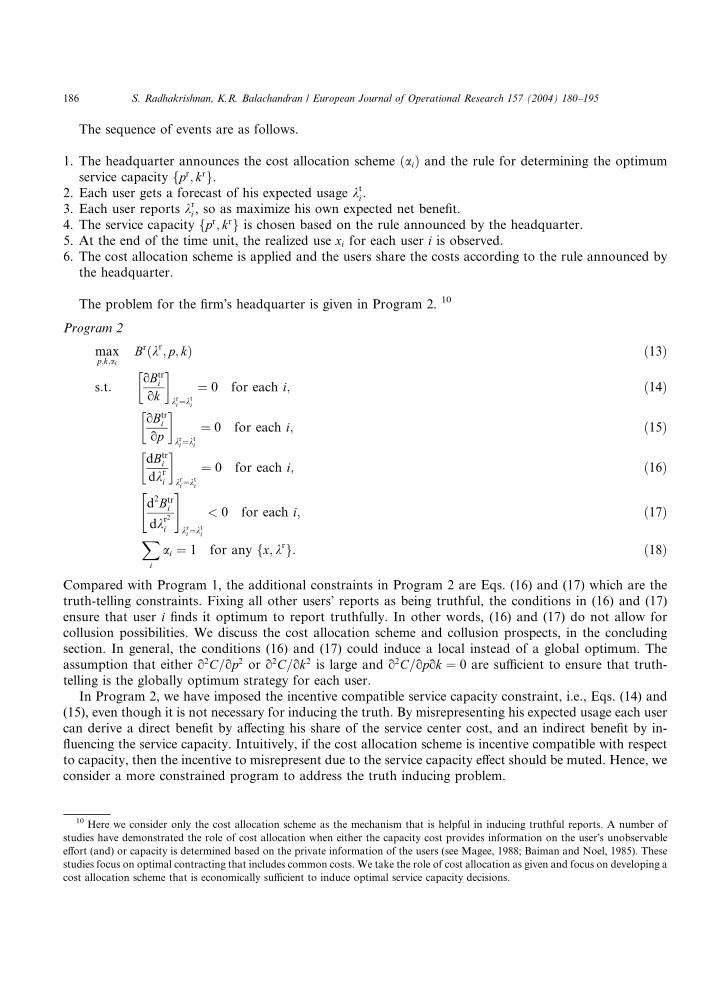
The sequence of events are as follows.

1. The headquarter announces the cost allocation scheme ðaiÞ and the rule for determining the optimum

service capacity fpr; krg.2. Each user gets a forecast of his expected usage kt

i .

3. Each user reports kri , so as maximize his own expected net benefit.

4. The service capacity fpr; krg is chosen based on the rule announced by the headquarter.

5. At the end of the time unit, the realized use xi for each user i is observed.6. The cost allocation scheme is applied and the users share the costs according to the rule announced by

the headquarter.

The problem for the firm�s headquarter is given in Program 2. 10

Program 2

10 H

studies

effort (

studies

cost al

maxp;k;ai

Brðkr; p; kÞ ð13Þ

s:t:oBtr

i

ok

� �kri¼kti

¼ 0 for each i; ð14Þ

oBtri

op

� �kri¼kti


dBtri

dkri

� �kri¼kti


d2Btri

dkr2

i

" #kri¼kti

< 0 for each i; ð17Þ

Xi

ai ¼ 1 for any fx; krg: ð18Þ

Compared with Program 1, the additional constraints in Program 2 are Eqs. (16) and (17) which are the

truth-telling constraints. Fixing all other users� reports as being truthful, the conditions in (16) and (17)

ensure that user i finds it optimum to report truthfully. In other words, (16) and (17) do not allow forcollusion possibilities. We discuss the cost allocation scheme and collusion prospects, in the concluding

section. In general, the conditions (16) and (17) could induce a local instead of a global optimum. The

assumption that either o2C=op2 or o2C=ok2 is large and o2C=opok ¼ 0 are sufficient to ensure that truth-

telling is the globally optimum strategy for each user.

In Program 2, we have imposed the incentive compatible service capacity constraint, i.e., Eqs. (14) and

(15), even though it is not necessary for inducing the truth. By misrepresenting his expected usage each user

can derive a direct benefit by affecting his share of the service center cost, and an indirect benefit by in-

fluencing the service capacity. Intuitively, if the cost allocation scheme is incentive compatible with respectto capacity, then the incentive to misrepresent due to the service capacity effect should be muted. Hence, we

consider a more constrained program to address the truth inducing problem.

ere we consider only the cost allocation scheme as the mechanism that is helpful in inducing truthful reports. A number of

have demonstrated the role of cost allocation when either the capacity cost provides information on the user�s unobservableand) or capacity is determined based on the private information of the users (see Magee, 1988; Baiman and Noel, 1985). These

focus on optimal contracting that includes common costs. We take the role of cost allocation as given and focus on developing a

location scheme that is economically sufficient to induce optimal service capacity decisions.


3.2. Development of the cost allocation scheme

Consider the following cost allocation scheme:

ai ¼vixi

vikri þP

j 6¼i vjkrj

þ vikri

vikri þP

j 6¼i vjkrj

1ð �P

j vjxjvik

ri þP

j 6¼i vjkrj

!: ð19Þ

Note that for any fx; krg,
Xi
ai ¼Xi

vixivik

ri þP

j 6¼i vjkrj

"þ vik

ri

vikri þP

j 6¼i vjkrj

1ð �P

j vjxjvik

ri þP

j 6¼i vjkrj

!#

¼P

i vikriP

j vjkrj

þP

i vixi � P

j vjkrj

� �P

i vikri

� Pj vjxj

� P

j vjkrj

� 2264

375 ¼ 1:

Thus, the constraint (18) is satisfied by the proposed scheme.If the expected cost allocation scheme given in Eq. (19) is based on average costs, then the first-best

capacity choice and truthful reports would also lead to each user�s expected net benefit being maximized

(see Proposition 1). As discussed earlier this should help to mute the indirect benefit of misrepresenting

expected usage by influencing the level of service capacity. The expected allocation to user i, given that all

other users report their expected usage truthfully, i.e., kj ¼ krj ¼ kt

j for j ¼ 1; . . . ; n and j 6¼ i is

Ex½ai� ¼vik

ti

vikri þP

j6¼i vjkjþ vik

ri

vikri þP

j 6¼i vjkj1�

vikti þP

j 6¼i vjkj

vikri þP

j 6¼i vjkj

!

¼ vikti

vikri þP

j6¼i vjkjþ

vikri vik

ri � vik

ti

�vik

ri þP

j 6¼i vjkj

� 2¼

vikti

Pj 6¼i vjkj þ v2i k

r2i

vikri þP

j 6¼i vjkj

� 2 :

ð20Þ

Evaluating Eq. (20) at kri ¼ kt

i we have

½Exfaig�kri¼kti¼ vik

ti

ðvikti þP

j6¼i vjkjÞ¼ di; ð21Þ

where to get the last equality compare (21) with (11). Thus, the expected cost allocation given truth-telling

by each user is based on average costs, and hence, should help to mute the incentives for misrepresentation.

The way the scheme operates is described below. (1) The firm�s headquarter announces the cost allo-

cation scheme as given in Eq. (19). The rule for determining the optimum service capacity fpr; krg is given as

the solution to

oBrðkr; pr; krÞop

¼ 0; ð22Þ

oBrðkr; pr; krÞok

¼ 0: ð23Þ

(2) Each user forecasts his expected usage to be kti and reports kr

i . (3) Based on (22) and (23), fpr; krg are

chosen. The service capacity cost is Cðpr; krÞ ¼ F þ cðpr; krÞ. (4) A charge per realized use for any user is


determined as R ¼ Cðpr; krÞ=½P

i vikri �. (5) In the first-tier, given the number of uses by user i to be xi, he is

charged viRxi.11(6) Let Y ¼ Cðpr; krÞ �

Pi viRxi, i.e., Y denotes the extent to which the service capacity cost

has not been charged to the users. If Y > 0, then the service capacity cost has not been fully recovered from

the users and if Y < 0, the service capacity cost is smaller than the cost recovered from the users. (7) In the

second-tier, each user i bears or is credited an amount ðYvikri Þ=P

i vikri .

The idea behind this cost allocation scheme is developed below. User i can either under-report or over-

report the true expected usage. If user i over-reports, the service capacity is higher and hence, the cost of

providing the service capacity is also higher. By over-reporting expected usage the charge for every realizeduse is reduced and an indirect effect is through the decreased expected delay. User i would not expect all the

service capacity costs to be charged in the first-tier. In the second-tier, the cost allocation scheme disposes

this under-charge to all users in the proportion of the reported usage. Thus, user i will bear a larger

proportion of the under-charge. Note that the other users also benefit from user i�s over-reporting.

However, if the charge in the second-tier is large enough for the user who over-reports, he can be dissuaded

from over-reporting. Similarly, when a user under-reports he decreases the service capacity and increases

the charge-out rate for every realized use. But the user who under-reports would expect that all the users

put together would be over-charged, in the first-tier. Hence, the user who under-reports would expect to geta credit for the over-charge. However, since he has under-reported expected usage, the credit is decreased,

in the second-tier. Thus, the user who under-reports will be charged more in the first-tier but get less credit

in the second-tier. The cost allocation scheme in Eq. (19) exactly balances these two effects and thus induces

each user to report his expected usage truthfully. The balancing of these effects is illustrated in the next

section with a numerical example.

We formally examine the solution to Program 2 and state the result in the following Proposition.

Proposition 2. The optimum service capacity in Program 2 is the same as the optimum service capacity in

Program 0, if the cost allocation scheme is given by Eq. (19).

Proof. See Appendix A.

Whang (1989) examines a model with information asymmetry and shows that a cost allocation based on

average costs induces truth-telling. There are three main assumptions in Whang (1989): (a) the delay costs

are homogenous of degree zero, (b) the capacity cost is linear and (c) the users private information is on

actual usage. Our model relaxes all these assumptions. Allocating costs based on average costs is similar todi. We can show that in the scenario examined here an allocation based on reported average costs alone, i.e.,

di is not sufficient.

3.3. Illustration of the cost allocation scheme

We illustrate the cost allocation scheme by considering an M/M/1 queue with two users so as to keep the

model simple and obtain closed form solutions. The expected usage of user 1 can be either high, medium or

low, i.e., k1ðHÞ > k1ðMÞ > k1ðLÞ. The expected usage of user 2 is k2. Hence, the truth inducing problem isrestricted to user 1�s report alone. The expected service rate is given by l and the service capacity cost is

C ¼ F þ hl. The expected net benefit for user 1 is

11 Even though the cost allocation scheme can be applied in one step after the realized use is observed, we split the description of the

cost allocation scheme into two-tiers to highlight the difference between the general procedure described in the managerial accounting

texts and our scheme.

Table

Numer

kr1

Pan

Whe

2.75

3.00

3.25

Whe

2.75

3.00

3.25

Whe

2.75

3.00

3.25

Pan

Whe

2.75

3.00

3.25

Whe

2.75

3.00

3.25

Whe

2.75

3.00

3.25

Param


Btr1 ¼ kt

1½g1 � v1W tr� � v1kt1v2k2 þ v21k

r2

1

ðv1kr1 þ v2k2Þ2

" #C; ð24Þ

where W tr ¼ 1=ðl � kt1 � k2Þ. The expected net benefit for user 2 is

Btr2 ¼ kt

2½g2 � v2W tr� � 1½ � v1kt1v2k2 þ v21k

r2

1

ðv1kr1 þ v2k2Þ2

#C: ð25Þ

The expected net benefit for the headquarter given any kr1 is

Br ¼ kr1½g1 � v1W r� þ k2½g2 � v2W r� � C: ð26Þ

The headquarter chooses the optimum service capacity by setting oBr=ol ¼ 0. For any reported expected

usage kr1, the optimal service rate is

lr ¼ f½v1kr1 þ v2k2�

12=h

12g þ ðkr

1 þ k2Þ: ð27Þ

1

ical example illustrating the cost allocation scheme

lr Cr W tr Charge/

use

User 1 User 2

E[Tier 1] E[Tier 2] Btr1 E[Tier 1] E[Tier 2] Btr

2

el A: High fixed cost, F¼ 60

n kt1 ¼ 2:75

7.446 74.891 0.590 13.025 35.818 0.000 3.811 39.074 0.000 4.157

7.732 75.464 0.504 12.577 34.588 1.572 3.702 37.732 1.572 4.182

8.018 76.036 0.441 12.166 33.456 3.163 3.412 36.497 2.920 4.260

n kt1 ¼ 3:00

7.446 74.891 0.692 13.025 39.074 �1.557 5.408 39.074 �1.669 5.550

7.732 75.464 0.577 12.577 37.732 0.000 5.536 37.732 0.000 5.536

8.018 76.036 0.496 12.166 36.497 1.582 5.435 36.497 1.460 5.556

n kt1 ¼ 3:25

7.446 74.891 0.836 13.025 42.330 �3.115 6.816 39.074 �3.398 6.815

7.732 75.464 0.675 12.577 40.876 �1.572 7.253 37.732 �1.572 6.816

8.018 76.036 0.566 12.166 39.538 0.000 7.373 36.497 0.000 6.806

el B: Low fixed cost, F¼ 6

n kt1 ¼ 2:75

7.446 20.891 0.590 3.633 9.991 0.000 29.637 10.900 0.000 32.331

7.732 21.464 0.504 3.578 9.838 0.447 29.578 10.732 0.447 32.307

8.018 22.036 0.441 3.526 9.696 0.917 29.425 10.577 0.846 32.254

n kt1 ¼ 3:00

7.446 20.891 0.692 3.633 10.900 �0.434 32.459 10.900 �0.474 32.500

7.732 21.464 0.577 3.578 10.732 0.000 32.536 10.732 0.000 32.536

8.018 22.036 0.496 3.526 10.577 0.458 32.478 10.577 0.423 32.513

n kt1 ¼ 3:25

7.446 20.891 0.836 3.633 11.808 �0.869 35.092 10.900 �0.948 32.539

7.732 21.464 0.675 3.578 11.626 �0.447 35.378 10.732 �0.447 32.691

8.018 22.036 0.566 3.526 11.458 0.000 35.453 10.577 0.000 32.726

eter values: g1 ¼ g2 ¼ 15; v1 ¼ v2 ¼ 1; k2 ¼ 3; h ¼ 2.


Table 1 demonstrates the intuition behind the cost allocation scheme. Here again we split the cost al-location scheme into two-tiers, which makes the intuition behind the scheme transparent. Note that the

scheme can be implemented in one step. We use the following parameter values for the numerical example:

v1 ¼ v2 ¼ 1, g1 ¼ g2 ¼ 15, k2 ¼ 3, k1ðHÞ ¼ 3:25, k1ðMÞ ¼ 3, k1ðLÞ ¼ 2:75, and h ¼ 2. In Panel A of Table 1,

F ¼ 60. Consider the case where the true expected usage is kt1 ¼ 3:00. If user 1 reports kr

1 ¼ 2:75, then the

optimum service rate based on the report is 7:446 (see Eq. (27)), the cost is 74:891 ¼ ½7:446� 2� þ 60, the

charge per use is 13:025 ¼ ½74:891=ð2:75þ 3:00Þ�. In the first-tier user 1 expects to be charged

39:074 ¼ ½13:025� 3:00� and also expects user 2 to be charged 39.074, with an expected total recovery in

the first-tier being 39:074þ 39:074 ¼ 78:148. Comparing this to the total cost of 74.891 the recoveryis higher than the cost by 3:297 ¼ 78:148� 74:891. In the second-tier the overcharge is credited to user 1

in the proportion of expected reported usage. Thus, in the second-tier user 1 expects to be credited

1:557 ¼ ½f2:75=2:75þ 3:00g � 3:297�. The expected waiting time is W tr ¼ 1=ðlr � kt1 � k2Þ ¼ ½1=ð7:446�

3:00� 3:00Þ� ¼ 0:692. The expected net benefit for user 1 is Btr1 ¼ 3:00� ½15� 0:692� � 39:074þ 1:557 ¼

5:407. Note that there are small rounding-off errors. By under-reporting the charge per use is higher, i.e.,

13.025 instead of 12.577 if user 1 reports truthfully. The total credit in the second-tier is 3.226, and user 1�sshare of the credit is only 1.557 leading to an expected net benefit of 5.408 as against 5.536 if he reports

truthfully. On the other hand, when user 1 over-reports (i.e., reports kr1 ¼ 3:25) the charge per realized use is

lower. But in the second-tier user 1 expects to bear a higher portion of the total under-charge. Hence, the

expected net benefit for user 1 is 5.435, instead of 5.536 if he reports truthfully.

The expected net benefit for user 2, who reports truthfully by default, is higher when user 1 misrepre-

sents; user 2�s expected net benefit is 5.550 when user 1 under-reports, 5.556 when user 1 over-reports and

5.536 when user 1 reports truthfully. Hence, it would appear that the cost allocation scheme penalizes the

user who misreports by increasing the expected net benefit of the other users. This leads us to examine the

next interesting question of whether user 2 will assist user 1 in obtaining good forecasts, such that he is not

‘‘hurt.’’

4. Incentives for obtaining good forecasts

In this section, we consider an M/M/1 queue with two users to provide insights into whether the cost

allocation scheme is sufficient to induce users (managers) to obtain good forecasts. The true expected usage

of user 1 is kt1 while the reported expected usage is kr

1 . The expected usage of user 2 is k2 and is common

knowledge. Hence, the truth inducing problem is restricted to user 1 alone. The expected service rate isgiven by l and the service capacity cost is C ¼ F þ hl. Thus, Btr

1 , Btr2 , B

r, and lr are as given by Eqs. (24)–

(27), respectively.

We want to examine if the cost allocation scheme provides incentives for user 2 to assist user 1 in ob-

taining good forecasts. We do this in two steps. First, we determine whether user 1�s truthful reporting

induced by the cost allocation scheme maximize or minimize the expected net benefit for user 2. 12 Second,

if user 1 has to exert effort to obtain the good forecasts, does the cost allocation scheme provide incentives

for user 1 to obtain good forecasts; and, are there any situations when user 2 will assist user 1 to obtain

good forecasts.

12 In the M/M/1 setting examined here it can be shown that Btr2 is globally convex/concave in kr1. For parsimony we focus our

discussion and derivations in the neighborhood of kr1 ¼ kt1.


4.1. Value of truth-telling for the other user

The expected net benefit for user 2 is given by

13 T

B2 ¼ g2k2 �v2k2

lr � kt1 � k2

� ½F þ hlr� 1� v1kt1v2k2 þ v21k

r2

1

ðv1kr1 þ v2k2Þ2

" #; ð28Þ

where lr is given by Eq. (27), and the cost allocation scheme is given by Eq. (19). Differentiating (28) with

respect to kr1, using (27) and evaluating at kr

1 ¼ kt1, we have, ½dB2=dkr

1�kr1¼kt1¼ 0. Thus, the expected net

benefit for user 2 either achieves a maximum or minimum when user 1 reports truthfully. Differentiating

again with respect to kr1 and evaluating at kr

1 ¼ kt1, we have

d2B2

dkr2

1

" #kr1¼kt

1

¼ F2v21v2k2

ðv1k1 þ v2k2Þ3

" #þ 3v21v2k2h

12

2ðv1k1 þ v2k2Þ52

" #� 2v1v2k

22hðv2 � v1Þ

ðv1k1 þ v2k2Þ3

" #� 2v2k2h

32

ðv1k1 þ v2k2Þ32

" #: ð29Þ

For large (small) fixed costs (F ), the expected net benefit of user 2 achieves a minimum (maximum), i.e.,

(29) is positive (negative). This is stated as a corollary.

Corollary 1. In the M/M/1 setting with the cost allocation scheme given by (19), the expected net benefit ofuser 2 achieves a minimum (maximum) if the fixed cost is high (low).

Proof. Direct from the derivation above. �

There are two effects of misrepresentation by user 1 on user 2�s expected net benefit. First, since the

service capacity is sub-optimal user 2 would face sub-optimal delays which would affect his expected net

benefit (i.e., the sub-optimal service capacity effect); and second, the cost allocation scheme penalizes user 1and hence, rewards user 2 for a bad forecast by user 1 (i.e., the cost allocation scheme effect). When the

fixed costs are low the cost allocation scheme effect is lower than the sub-optimal service capacity effect, and

user 2 is hurt by user 1�s misrepresentation; hence, there is value for user 1�s truth-telling to user 2. Table 1,

Panel A illustrates this effect when fixed costs are high and Table 1, Panel B illustrates the effect when fixed

costs are low, F ¼ 6.

4.2. Incentives for obtaining good forecasts

We extend the our model, by letting user 1 exert an unobservable effort to obtain good forecasts at a cost

of R per unit time before he observes the true expected usage. If user 1 exerts effort he observes kt1. User 1

can decide (a) not to exert the forecast effort, and use a randomized strategy to report expected usage; or (b)

to exert the forecast effort and report truthfully. The expected usage of user 1 can be either high, medium or

low, i.e., k1ðHÞ > k1ðMÞ > k1ðLÞ with a probability of /ðjÞ for j ¼ H ;M ; L. Consistent with the earlier

notation, let Bjk1 denote that user 1 has observed kt

1 ¼ k1ðjÞ and has chosen to report kr1 ¼ k1ðkÞ. For

the numerical example, we let /ðjÞ ¼ 1=3, R ¼ 0:12 and all other parameters are the same as in Table 1.

Table 2 provides the expected net benefit of user 1�s strategies for exerting forecast effort and not exert-ing forecast effort. Consider user 1�s strategy of not exerting forecast effort and reporting kr

1 ¼ k1ðkÞwith probability qðkÞ ¼ 1=3 for k ¼ H ;M ; L. 13 The expected net benefit with no forecast effort is

his randomized strategy is reasonable given that the user has no information other than /ðjÞ ¼ 1=3.

Table 2

Incentives for good forecasts

Bjk1 given no forecast effort Bjk

1 given forecast effort

kt1 ¼ 2:75 kt

1 ¼ 3:00 kt1 ¼ 3:25 kt

1 ¼ 2:75 kt1 ¼ 3:00 kt

1 ¼ 3:25

Panel A: High fixed cost, F ¼ 60

kr1 ¼ 2:75 3.811 5.408 6.816 3.811

kr1 ¼ 3:00 3.703 5.536 7.253 5.536

kr1 ¼ 3:25 3.419 5.435 7.373 7.373Pk B

jk1 qðkÞ 3.644 5.460 7.148 3.811 5.536 7.373P

j

Pk B

jk1 qðkÞ/ðjÞ ½ð3:644þ 5:460þ 7:148Þ=3� ¼ 5:471 ½ð3:811þ 5:536þ 7:373Þ=3� ¼ 5:573



kt1 ¼ 2:75 kt

1 ¼ 3:00 kt1 ¼ 3:25 kt

1 ¼ 2:75 kt1 ¼ 3:00 kt

1 ¼ 3:25

kr1 ¼ 2:75 4.157 5.550 6.815 4.157

kr1 ¼ 3:00 4.182 5.536 6.816 5.536

kr1 ¼ 3:25 4.260 5.556 6.806 6.806Pk B

jk2 qðkÞ 4.200 5.547 6.812 4.157 5.536 6.806P

j

Pk B


Panel B: Low fixed cost, F ¼ 6



kt1 ¼ 2:75 kt

1 ¼ 3:00 kt1 ¼ 3:25 kt

1 ¼ 2:75 kt1 ¼ 3:00 kt

1 ¼ 3:25

kr1 ¼ 2:75 29.637 32.459 35.092 29.637

kr1 ¼ 3:00 29.578 32.536 35.378 32.536

kr1 ¼ 3:25 29.425 32.478 35.453 35.453Pk B

jk1 qðkÞ 29.546 32.491 35.308 29.637 32.536 35.453P

j

Pk B




kt1 ¼ 2:75 kt

1 ¼ 3:00 kt1 ¼ 3:25 kt

1 ¼ 2:75 kt1 ¼ 3:00 kt

1 ¼ 3:25

kr1 ¼ 2:75 32.331 32.499 32.539 32.331

kr1 ¼ 3:00 32.307 32.536 32.691 32.536

kr1 ¼ 3:25 32.254 32.513 32.726 32.726Pk B

jk2 qðkÞ 32.297 32.516 32.652 32.331 32.536 32.726P

j

Pk B


Parameter values: g1 ¼ g2 ¼ 15; v1 ¼ v2 ¼ 1; k2 ¼ 3; h ¼ 2; M ¼ 0:12; /ðjÞ ¼ 1=3.

Without forecast effort user 1 reports kr1 ¼ k with probability 1/3, i.e., qðkÞ ¼ 1=3.

With forecast effort user 1 reports kr1 ¼ kt

1 ¼ j truthfully.

192

S.Radhakrish

nan,K.R.Balachandran/EuropeanJournalofOpera

tionalResea

rch157(2004)180–195


Pj

Pk B

jk1 /ðjÞqðkÞ ¼ 5:471. 14 The expected net benefit with forecast effort is

Pj B

jj1 /ðjÞ � R, where we

have used the result of Proposition 2 that truthful reporting is user 1�s best strategy once he has the in-

formation on the true expected usage. In general, user 1 will exert forecast effort if and only ifPj B

jj1 /ðjÞ �

Pj

Pk B

jk1 /ðjÞqðkÞPR. By concavity of B1 in kr

1 we have thatP

j Bjj1 /ðjÞ�P

j

Pk B

jk1 /ðjÞqðkÞ > 0. Also, from Corollary 1, it follows that

Pj B

jj2 /ðjÞ �

Pj

Pk B

jk2 /ðjÞqðkÞ > 0, when

the fixed costs are low, and vice-versa. Thus, when fixed costs are low there exist settings wherePj B

jj1 /ðjÞ �

Pj

Pk B

jk1 /ðjÞqðkÞ < R and

Pj B

jj2 /ðjÞ �

Pj

Pk B

jk2 /ðjÞqðkÞ > 0. We summarize this obser-

vation in the following corollary.

Corollary 2. In the M/M/1 setting with the two-tier cost allocation scheme, there exist cases when user 1 willnot be induced to exert forecast effort and user 2 finds it beneficial to assist user 1 to obtain good forecasts.

Proof. Direct from the derivation above. �

The corollary shows that while the cost allocation scheme on its own does not induce user 1 to exert

forecast effort, user 2 would assist user 1 to obtain good forecasts. This exploratory analysis suggests the

following interesting possibilities for future analysis: (a) Can the cost allocation scheme be modified toaccommodate the incentives for obtaining forecasts, such that the costs of sub-optimal service capacity are

shared in an equitable fashion? (b) Can other users modify their reported expected usage to compensate for

one user�s bad forecasts? (c) Can the problem of inducing good forecasts be decoupled with the reporting

problem?

5. Concluding remarks

In this paper, we examine a M/G/1 queue and develop a cost allocation scheme to allocate service ca-

pacity improvement cost among multiple users. The cost allocation scheme has some desirable properties.

Specifically, the cost allocation scheme (a) maximizes each user�s expected net benefit with respect to service

capacity, (b) induces each user to report expected usage truthfully (c) allocates all the service capacity costs

and (d) achieves the same service capacity as the headquarter would set if there was no private information

on expected usage. The cost allocation scheme is simple, in the sense that it uses only the reported expected

usage (similar to the budgeted or forecasted usage) and the realized usage, i.e., volume-driven cost drivers.

The cost allocation scheme does not depend on measurement of the realized waiting time, realized delaytime, the realized net benefits, etc. This is important because, in a lot of situations a direct measure of the

net benefits might be impossible to obtain without allocating the revenues of the final product. For ex-

ample, if the service is only one among various activities that is required to put together a product that is

sold to customers, then getting an estimate of the benefit of this service alone could be difficult, if not

impossible. We also highlight interesting questions relating to incentives across users.

Among the limitations of the cost allocation scheme that we develop is that it provides muted incentives

for obtaining good forecasts. Also, the cost allocation scheme does not directly address the possibility that a

14 Given that the true expected usage is kt1 ¼ 3:00 the user will report 2.75, 3.00 and 3.25 with equal probability. This gives an

expected benefit conditioned on kt1 ¼ 3:00, as 5.408 when kr1 ¼ 2:75, as 5.536 when kr1 ¼ 3:00, and as 5.435 when kr1 ¼ 3:25. These are

the Btr1 when kt1 ¼ 3:00 and kr1 ¼ 2:75, 3.00 and 3.25 and the derivation is similar to that in Panel A of Table 1. Given that qðkÞ ¼ 1=3,

the expected net benefit conditioned on kt1 ¼ 3:00 isP

k Bjk1 /ðjÞqðkÞ ¼ ½ð5:408þ 5:536þ 5:435Þ=3� ¼ 5:460. Similarly, conditioned on

kt1 ¼ 2:75 isP

k Bjk1 /ðjÞqðkÞ ¼ ½ð3:811þ 3:703þ 3:419Þ=3� ¼ 3:644; and conditioned on kt1 ¼ 3:25 is

Pk B

jk1 /ðjÞqðkÞ ¼ ½ð6:816þ 7:253þ

7:373Þ=3� ¼ 7:148.


group of users could get together and decide to game the allocation scheme to their collective benefit. Thatis, we have not examined the possibility of collusion among classes. Since costs are allocated in its entirety,

collusion is not possible in the case of two classes. With more than two classes, colluding classes can,

theoretically, be combined into one class and the scheme will work. However, the scheme may not work

when collusion prospects are not known to headquarters, thus not enabling combining of classes.

Appendix A. Proof of propositions

A.1. Proof of Proposition 1

Denote the optimum of Program 1 by fp ; k g. The constraints (8) and (9) are

oBiðk; p; k; diÞop

¼ � kivioW ðk; p; kÞ

op

� ��þ di

oCðp; kÞop

�¼ 0; ðA:1Þ

oBiðk; p; k; diÞok

¼ � kivioW ðk; p; kÞ

ok

� ��þ di

oCðp; kÞok

�¼ 0; ðA:2Þ

for each i. Using (4) in (A.1) and (5) in (A.2) it follows that p ¼ p and k ¼ k , if and only if di is chosen

as in (11). The di given by (11) satisfies (10). �

A.2. Proof of Proposition 2

We need to show that with the proposed cost allocation scheme leads to the solution of Program 2 with

kri ¼ kt

i for each i, p ¼ p and k ¼ k , where fp; kg represents the optimum service capacity for Program 2.

We will show that the conjectured solution is feasible, i.e., satisfies the constraints in Program 2.

First, we show that from the perspective of user i, truth-telling is the optimum strategy, given that the

other users report truthfully. Thus, we let kj ¼ krj ¼ kt

j for any j 6¼ i and show that constraints (16) and (17)

are satisfied for any i, with the cost allocation scheme ai given that the other users report truthfully. Theexpected net benefit per unit time for user i is

Btri ¼ kt

i ½gi � viW tr� � GiCðpr; krÞ;
where
Gi ¼ Exfaig:
It follows that
dBtri

dkri

¼ oBtri

oprdpr

dkri

þ oBtri

okrdkr

dkri

þ oBtri

okri

¼ oBtri

oprdpr

dkri

þ oBtri

okrdkr

dkri

� oGi

okri

Cðpr; krÞ½ �;ðA:3Þ

where we have used oBtri =ok

ri ¼ �ðoGi=ok

ri Þ½Cðpr; krÞ�. Noting that ½Gi�kri¼kti

¼ di (see Eq. (21)), using Eqs.

(22) and ( 23) and following the same track as in the proof of Proposition 1, it follows that ½oBtri =op�kri¼kti

¼ 0

and ½oBtri =ok�kri¼kti

¼ 0 that is the constraints (14) and (15) are satisfied.Noting that ½oGi=ok

ri ¼ ð2C

Pj6¼i vjkjviðkt

i � kri ÞÞ=ðvik

ri þP

j 6¼i vjkjÞ3�, using ½oBtri =op�kri¼kti

¼ 0 and ½oBtri =

ok�kri¼kti¼ 0 we get ½dBtr

i =dkri �kri¼kti

¼ 0. Thus, constraint (16) is satisfied.


To verify that constraint (17) is satisfied, we have that

d2Btri

dkr2

i

¼ � vikti

o2W tr

opr2

� ��þ Gi

o2Copr2

� ��dpdkr

i

� �2� oBtr

i

opr

� �d2pr

dkr2

i

" #� vik

ti

o2W tr

okr2

� ��

þ Gio2Cokr2

� ��dkdkr

i

� �2� oBtr

i

okr

� �d2kr

dkr2

i

" #� vik

ti

o2W tr

oprokr

� ��þ Gi

o2Coprokr

� ��dpr

dkri

dkr

dkri

� �

�6CP

j 6¼i vjkjviðkti � kr

i Þðvikr

i þP

j 6¼i vjkjÞ2�

2CP

j 6¼i vjkj

ðvikri þP

j 6¼i vjkjÞ3: ðA:4Þ

We can show that dpr=dkri > 0 and dkr=dkr

i > 0 by using Eqs. (22) and (23) and the second-order conditions

for optimality. Using Eq. (12) we get o2W tr=opr2> 0, o2W tr=okr

2> 0, and o2W tr=oprokr > 0. Using these

relations, the assumption of o2C=opr2 > 0, o2C=okr2 > 0, o2C=oprokr ¼ 0, ½oBtri =op

r�kri¼kti¼ 0 and

½oBtri =ok

r�kri¼kti¼ 0 we get ½d2Btr

i =dkr2

i �kri¼kti< 0. Thus, the cost allocation scheme satisfies constraint (17).

From eq. (19) we haveP

i ai ¼ 1, for any fx; krg and thus constraint (18) is satisfied.

Noting that ½Gi�kri¼kti¼ di (see Eq. (21)) and following the same track as in the proof of Proposition 1, it

follows that the optimum fp; kg is the same as in Program 0. �

References

Baiman, S., Noel, J., 1985. Non-controllable costs and responsibility accounting. Journal of Accounting Research 23, 230–245.

Balachandran, K.R., Radhakrishnan, S., 1994. Extensions to class dominance characteristics. Management Science 40, 1353–1360.

Balachandran, K.R., Schaefer, M.E., 1979. Class dominance characteristics at a service facility. Econometrica 47, 515–519.

Balachandran, K.R., Schaefer, M.E., 1980. Public and private optimization at a service facility with approximate information on

congestion. European Journal of Operations Research 4, 195–202.

Barefield, J., Raiborn, C., Kinney, M., 1994. Cost Accounting: Traditions and Innovations, second ed. West Publishing, St. Paul

Minnesota.

Cooper, R.B., 1981. Introduction to Queuing Theory. Elsevier, New York.

Foster, G., Gupta, M., 1990. Manufacturing overhead cost driver analysis. Journal of Accounting and Economics 12, 309–337.

Fudenberg, D., Tirole, J., 1998. Game Theory. The MIT Press, Cambridge, MA.

Groves, T., Ledyard, J., 1980. The existence of efficient and incentive compatible equilibria with public good. Econometrica 48, 1487–1506.

Groves, T., Loeb, M., 1979. Incentives in a divisionalized firm. Management Science 24, 221–230.

Holmstrom, B., 1979. Groves� schemes on restricted domains. Econometrica 47, 1137–1144.

Horngren, C.T., Foster, G., Datar, S.M., 2000. Cost Accounting: A Managerial Emphasis, 10th ed. Prentice Hall, Upper Saddle River,

NJ.

Karmarker, U.S., Kekre, S., Kekre, S., 1985a. Lot sizing in multi-machine job shops. IIE Transactions 17, 290–298.

Karmarker, U.S., Kekre, S., Kekre, S., Freeman, S., 1985b. Lot sizing and lead time performance in a manufacturing cell. Interfaces

15, 1–9.

Laffont, J., Maskin, E., 1980. A differential approach to dominant strategy mechanisms. Econometrica 48, 1507–1520.

Magee, P., 1988. Variable cost allocation in a principal–agent setting. The Accounting Review 63, 42–53.

Mendelson, H., Whang, S., 1990. Optimal incentive compatible priority pricing for the M/M/1 queue. Operations Research 38, 870–883.

Mendelson, H., Whang, S., 1994. Pricing for communications network service. Working paper, Graduate School of Business, Stanford

University, CA.

Miller, B.L., Buckman, A.G., 1987. Cost allocation and opportunity costs. Management Science 33, 626–639.

Radhakrishnan, S., Balachandran, K.R., 1995. Delay costs and incentive schemes for multiple users. Management Science 41, 646–652.

Radhakrishnan, S., Balachandran, K.R., 1996. Cost of congestion, operational efficiency and management accounting. European

Journal of Operations Research 89, 237–245.

Ronen, J., 1992. Transfer pricing reconsidered. Journal of Public Economics 47, 125–136.

Ronen, J., McKinney III, G., 1970. Transfer pricing for divisional autonomy. Journal of Accounting Research 18, 99–112.

Walker, M., 1980. On the non existence of a dominant strategy mechanism for making optimal public decisions. Econometrica 48,

1521–1540.

Whang, S., 1989. Cost allocation revisited: An optimality result. Management Science 35 (10), 1264–1273.

service capacity decision and incentive compatible cost allocation for reporting usage forecasts

Documents