seroprevalence with uncertainty - dash home

Estimating SARS-CoV-2 seroprevalenceand epidemiological parameters withuncertainty from serological surveys

The Harvard community has made thisarticle openly available. Please share howthis access benefits you. Your story matters

Citation Larremore, Daniel B., Bailey K. Fosdick, Kate M. Bubar, Sam Zhang,Stephen M. Kissler, et al. Estimating SARS-CoV-2 seroprevalenceand epidemiological parameters with uncertainty from serologicalsurveys (2020).

Citable link http://nrs.harvard.edu/urn-3:HUL.InstRepos:42659939

Terms of Use This article was downloaded from Harvard University’s DASHrepository, and is made available under the terms and conditionsapplicable to Other Posted Material, as set forth at http://nrs.harvard.edu/urn-3:HUL.InstRepos:dash.current.terms-of-use#LAA

http://osc.hul.harvard.edu/dash/open-access-feedback?handle=&title=Estimating%20SARS-CoV-2%20seroprevalence%20and%20epidemiological%20parameters%20with%20uncertainty%20from%20serological%20surveys&community=1/4454687&collection=1/4454688&owningCollection1/4454688&harvardAuthors=d520ed0d49c307c6d0b1c81c0aeeb14f&department

http://nrs.harvard.edu/urn-3:HUL.InstRepos:42659939

http://nrs.harvard.edu/urn-3:HUL.InstRepos:dash.current.terms-of-use#LAA



Estimating SARS-CoV-2 seroprevalence andepidemiological parameters with uncertainty from

serological surveys

Daniel B. Larremore,1,2∗ Bailey K. Fosdick,3 Kate M. Bubar4,5,Sam Zhang4, Stephen M. Kissler6, C. Jessica E. Metcalf,7

Caroline O. Buckee8,9, Yonatan H. Grad6∗

1Department of Computer Science, University of Colorado Boulder, Boulder, CO, 80309, USA2BioFrontiers Institute, University of Colorado Boulder, Boulder, CO, 80303, USA3Department of Statistics, Colorado State University, Fort Collins, CO, 80523, USA

4Department of Applied Mathematics, University of Colorado Boulder, Boulder, CO, 80303, USA5IQ Biology Program, University of Colorado Boulder, Boulder, CO, 80309, USA

6Department of Immunology and Infectious Diseases,

Harvard T.H. Chan School of Public Health, Boston, MA, 02115, USA7Department of Ecology and Evolutionary Biology and the Woodrow Wilson School,

Princeton University, Princeton, NJ, 08540, USA8Department of Epidemiology,

Harvard T.H. Chan School of Public Health, Boston, MA, 02115, USA9Center for Communicable Disease Dynamics,

Harvard T.H. Chan School of Public Health, Boston, MA, 02115, USA

∗To whom correspondence should be addressed;E-mail: [email protected] and [email protected].

Establishing how many people have already been infected by SARS-CoV-2 is

an urgent priority for controlling the COVID-19 pandemic. Patchy virolog-

ical testing has hampered interpretation of confirmed case counts, and un-

known rates of asymptomatic and mild infections make it challenging to de-

1

velop evidence-based public health policies. Serological tests that identify past

infection can be used to estimate cumulative incidence, but the relative accu-

racy and robustness of various sampling strategies has been unclear. Here,

we used a flexible framework that integrates uncertainty from test charac-

teristics, sample size, and heterogeneity in seroprevalence across tested sub-

populations to compare estimates from sampling schemes. Using the same

framework and making the assumption that serological positivity indicates

immune protection, we propagated these estimates and uncertainty through

dynamical models to assess the uncertainty in the epidemiological parameters

needed to evaluate public health interventions. We examined the relative accu-

racy of convenience samples versus structured surveys to estimate population

seroprevalence, and found that sampling schemes informed by demograph-

ics and contact networks outperform uniform sampling. The framework can

be adapted to optimize the design of serological surveys given particular test

characteristics and capacity, population demography, sampling strategy, and

modeling approach, and can be tailored to support decision-making around

introducing or removing interventions.

2

Introduction

Serological testing is a critical component of the response to COVID-19 as well as to future

epidemics. Assessment of population seropositivity, a measure of the prevalence of individuals

who have been infected in the past and developed antibodies to the virus, can address gaps in

knowledge of the cumulative disease incidence. This is particularly important given inadequate

viral diagnostic testing and incomplete understanding of the rates of mild and asymptomatic

infections (1). In this context, serological surveillance has the potential to provide information

about the true number of infections, allowing for robust estimates of case and infection fatality

rates and for the parameterization of epidemiological models to evaluate the possible impacts

of specific interventions and thus guide public health decision-making.

The proportion of the population that has been infected by, and recovered from, the coro-

navirus causing COVID-19 will be a critical measure to inform policies on a population level,

including when and how social distancing interventions can be relaxed. Individual serological

testing may allow low-risk individuals to return to work, school, or college, contingent on the

immune protection afforded by a measurable antibody response. At a population level, however,

methods are urgently needed to design and interpret serological data based on testing of sub-

populations, including convenience samples that are likely to be tested first, to reliably estimate

population seroprevalence.

Three sources of uncertainty complicate efforts to learn population seroprevalence from sub-

sampling. First, tests may have imperfect sensitivity and specificity; estimates for COVID-19

tests on the market as of April 2020 reported specificity between 95% and 100% and sensitivity

between 62% and 97% (Supplementary Table S1). Second, the population sampled will likely

not be a representative random sample, particularly in the first rounds of testing, when there is

urgency to test using convenience samples and potentially limited serological testing capacity.

3

Third, there is uncertainty inherent to any model-based forecast which uses the empirical esti-

mation of seroprevalence, regardless of the quality of the test, in part because of the uncertain

relationship between seropositivity and immunity (2).

A clear evidence-based guide to aid the design of serological studies is critical to policy

makers and public health officials both for estimation of seroprevalence and for forward-looking

modeling efforts, particularly if serological positivity reflects immune protection. To address

this need, we developed a framework that can be used to design and interpret serological studies,

with applicability to SARS-CoV-2. Starting with results from a serological survey of a given

size and age stratification, the framework incorporates the test’s sensitivity and specificity and

enables estimates of population seroprevalence that include uncertainty. These estimates can

then be used in models of disease spread to calculate the effective reproductive number Reff, the

transmission potential of SARS-CoV-2 under partial immunity, to forecast disease dynamics,

and to assess the impact of candidate public health and clinical interventions. Similarly, starting

with a pre-specified tolerance for uncertainty in seroprevalence estimates, the framework can

be used to define the sample size needed. This framework can be used in conjunction with any

model, including ODE models (3, 4), agent-based simulations (5), or network simulations (6),

and can be used to estimate Reff or to simulate transmission dynamics.

Results

The overall framework is described in Fig. 1, showing that the workflow can be used in two

directions. In the forward direction, starting from serological data, one can estimate seropreva-

lence. While valuable on its own, seroprevalence can also be used as the input to an appropriate

model to update forecasts or estimate the impacts of interventions. In the reverse direction, sam-

ple sizes can be calculated to yield estimates with a desired level of uncertainty and efficient

sampling strategies can be developed based on prospective modeling tasks.

4

Test sensitivity/specificity, sampling bias, and true seroprevalence influence the accuracy

and robustness of estimates. To integrate uncertainty arising from test sensitivity and speci-

ficity, we produced a Bayesian posterior distribution of seroprevalence that accommodates un-

certainty associated with a finite sample size (Fig. 1; green annotations). We denote the posterior

probability that the true population serology is equal to θ, given test outcome data X and test

sensitivity and specificity characteristics, as Pr(θ | X). Because sample size and outcomes are

included in X , and because test sensitivity and specificity are included in the calculations, this

posterior distribution over θ appropriately handles uncertainty (see Methods).

To illustrate the use of these calculations in practice, we first simulated serological data from

populations with seroprevalence rates ranging from 1% to 50% using the reported sensitivity

(93%) and specificity (97.5%) of a test approved for sale in the EU (Supplementary Table S1),

and with the number of samples ranging from 100 to 5000. Next, we constructed Bayesian pos-

terior estimates of seroprevalence (see Methods), finding that, when seroprevalence is 10% or

lower, around 1000 samples are necessary to estimate seroprevalence to within two percentage

points (Fig. 2). Tests with other characteristics required around 1000 tests (93.8% sensitivity,

97.5% specificity; Supplementary Fig. S1A) and 750 tests (97.2% sensitivity and 100% speci-

ficity; Supplementary Fig. S1B) to achieve the same uncertainty levels, relative to the minimum

of around 650 tests for a theoretical test with perfect sensitivity and specificity (Supplementary

Fig. S1C).

Sampling frameworks for seropositivity estimates are likely to be non-random and con-

strained to subpopulations. Therefore, although general estimates were most uncertain when

true seropositivity was near 50%, the number of samples was low, and/or test sensitivity/specificity

were low (Fig. 2 and Supplementary Fig. S1), another source of statistical uncertainty comes

from the potentially uneven distribution of samples across a population with variation in true

positivity. To extrapolate seropositivity from a sample of a particular subpopulation, we speci-

5

fied a Bayesian hierarchical model by introducing a common prior distribution on subpopulation-

specific seropositivities θi (see Methods). In effect, this allowed seropositivity estimates from

individual subpopulations to inform each other while still taking into account subpopulation-

specific testing outcomes.

Convenience sampling (testing blood samples that were obtained for another purpose and

are readily available) will often be the easiest and quickest data collection method (7). Two

examples of such convenience samples are newborn heel stick dried blood spots, which contain

maternal antibodies and thus reflect maternal exposure, and serum from blood donors. Sam-

pling may also be designed to represent a broader range of the population, such as random

uniform sampling across age groups, sampling informed by population demographics, or sam-

pling in relation to expectations about contribution to transmission, for example based on an

age-structured contact matrix (8–10). We termed this latter sampling scheme ‘model and de-

mographics informed’ sampling.

We tested the ability of the Bayesian hierarchical model described above to infer both pop-

ulation and subpopulation seroprevalence, even when only a convenience sample was available.

The credible interval in the resulting overall seroprevalence estimates were influenced by the

age demographics sampled, with the most uncertainty in the newborn dried blood spots sample

set, due to the narrow age range for the mothers (Fig. 3). For such sampling strategies, which

draw from only a subset of the population, our mathematical approach assumes that seropreva-

lence in each subpopulation does not dramatically vary and thus infers that seroprevalence in the

unsampled bins is similar to that in the sampled bins but with increased uncertainty (Methods;

Supplementary Text). Uncertainty was also influenced by the overall seroprevalence, such that

the width of the 90% credible interval increased with higher seroprevalence for a given sample

size. While test sensitivity and specificity also impacted uncertainty, central estimates of overall

seropositivity were robust for sampling strategies that spanned the entire population.

6

Seroprevalence estimates inform uncertainty in epidemic peak and timing. As a natu-

ral extension to use of serological data to estimate core epidemiological quantities (11–13) or

to map out patterns of outbreak risk (14), the posterior distribution of seroprevalence can be

used as an input to any epidemiological model, including a typical SEIR model (3), where the

proportion seropositive may correspond to the recovered/immune compartment, or a more com-

plex framework such as an age-structured SEIR model incorporating interventions like closing

schools and social distancing (10,15) (Fig. 1; blue annotations). We integrated uncertainty in the

posterior estimates of seroprevalence and uncertainty in model dynamics or parameters using

Monte Carlo sampling to produce a posterior distribution of trajectories or key epidemiological

parameter estimates (Fig. 1; black annotations).

Figure 4 illustrates how estimates of the height and timing of peak infections varied under

two serological sampling scenarios and two hypothetical social distancing policies for a ba-

sic SEIR framework parameterized using seroprevalence data. Uncertainty in seroprevalence

estimates propagated through SEIR model outputs in stages: larger sample sizes at a given

seroprevalence resulted in a smaller credible interval for the seroprevalence estimate, which

improved the precision of estimates of both the height and timing of the epidemic peak. In

this case, we assumed the same serological test sensitivity and specificity as before (93% and

97.5%, respectively), but test characteristics also impacted model estimates, with more specific

and sensitive tests leading to more precise estimates (Supplementary Fig. S3). Even estima-

tions from a perfect test carried uncertainty, which corresponds to the size of the sample set

(Supplementary Fig. S3).

For convenience samples from particular age groups or age-stratified serological surveys,

the Bayesian hierarchical model extrapolates seroprevalence in sampled subpopulations to the

overall population, with uncertainty propagated from these estimates to model-inferred epi-

demiological parameters of interest, such as Reff. Estimates from 1000 neonatal heel sticks or

7

blood donations achieved more uncertain, but still reasonable, estimates of overall seropreva-

lence and Reff as compared to uniform or demographically informed sample sets (Fig. 5). Here,

convenience samples produced higher confidence estimates in the tested subpopulations, but

high uncertainty estimates in unsampled populations through our Bayesian modeling frame-

work. In all scenarios, our framework propagated uncertainty appropriately from serological

inputs to estimates of overall seroprevalence or Reff. Improved test sensitivity and specificity

correspondingly improved estimation and reduced the number of samples that would be re-

quired to achieve the same credible interval for a given seroprevalence, and would similarly

reduce the sampling needed to equivalent estimation of Reff (Supplementary Figs. S5 and S7).

If the subpopulation in the convenience sample has a systematically different seroprevalence

from the general population, increasing the sample size may bias estimates (Supplementary

Figs. S4 and S7). This can be avoided using data from other sources or by updating the Bayesian

prior distributions with known or hypothesized relationships between seroprevalence of the

sampled and unsampled populations.

Strategic sample allocation improves estimates. The flexible framework described in Fig. 1

enables the calculation of sample sizes for different serological survey designs. To calculate

the number of tests required to achieve a seroprevalence estimate with a specified tolerance for

uncertainty, and to allocate tests according to a specific subpopulation or in the context of a

particular intervention, we treated the eventual estimate uncertainty as a framework output and

then sought to minimize it by improving the allocation of samples (Fig. 1, dashed arrow).

Uniform allocation of samples across subpopulations is not always optimal; it can be im-

proved upon by i) increasing sampling in subpopulations with higher seroprevalence, and ii)

increasing sampling in subpopulations with higher relative influence on the quantity to be es-

timated. This approach, which we termed model and demographics informed (MDI), allocates

8

samples to subpopulations in proportion to how much sampling them would decrease the pos-

terior variance of estimates, i.e, ni ∝ xi√θ∗i (1− θ∗i ), where θ∗i = 1− sp + θi(se + sp + 1) is the

probability of a positive test in subpopulation i given test sensitivity (se), test specificity (sp),

and subpopulation seroprevalence θi, and xi is the the relative importance of subpopulation i to

the quantity to be estimated. When that quantity is overall seroprevalence, xi is the fraction of

the population in subpopulation i; when that quantity is total infections orReff, xi can be derived

from the structure of the model itself (see Methods). If subpopulation prevalence estimates θi

are unknown, sample allocation based solely on xi is recommended.

To demonstrate the effects of MDI sample allocation, we used it to design a strategy to

optimize estimates of Reff and then tested the performance of its sample allocations against

those of blood donations, neonatal heel sticks, and uniform sampling. MDI produced higher

confidence posterior estimates (Fig. 5J, Supplementary Fig. S7). Importantly, because the rela-

tive importance of subpopulations in a model may vary based on the hypothetical interventions

being modeled (e.g., the re-opening of workplaces would place higher importance on the sero-

logical status of working-age adults), MDI sample allocation recommendations may have to be

derived for multiple hypothetical interventions and then averaged to design a study from which

the largest variety of high-confidence results can be derived. To see how such recommenda-

tions would work in practice, we computed MDI recommendations to optimize three scenarios

for the contact patterns and demography of the U.S. and India, deriving a balanced sampling

recommendation (Fig. 6).

Discussion

There is a critical need for serological surveillance of SARS-CoV-2 to estimate cumulative inci-

dence. Here, we presented a formal framework for doing so to aid in the design and interpreta-

tion of serological studies. We considered that sampling may be done in varying ways, including

9

broad initial efforts to approximate seroprevalence using convenience samples, as well as more

complex and resource-intensive structured sampling schemes, and that these efforts may use

one of any number of serological tests with distinct test characteristics. We further incorpo-

rated into this framework an approach to propagating the estimates and associated uncertainty

through mathematical models of disease transmission (focusing on scenarios where seropreva-

lence maps to immunity) to provide decision-makers with tools to evaluate the potential impact

of interventions and thus guide policy development and implementation.

Our results suggest approaches to serological surveillance that can be adapted as needed

based on pre-existing knowledge of disease prevalence and trajectory, availability of conve-

nience samples, and the extent of resources that can be put towards structured survey design

and implementation.

In the absence of baseline estimates of seroprevalence, an initial survey will provide a pre-

liminary estimate of population prevalence (Fig. 2). Our framework updates the ‘rule of 3’

approach (16) by incorporating uncertainty in test characteristics and can further address un-

certainty from biased sampling schemes (see Supplementary Text). As a result, convenience

samples, such as newborn heel stick dried blood spots or samples from blood donors, can be

used to estimate population seroprevalence. However, it is important to note that in the ab-

sence of reliable assessment of correlations in seroprevalence across age groups, extrapolations

from these convenience samples may be misleading as sample size increases (Supplementary

Figs. S4 and S6). Uniform or model and demographic informed samples, while more challeng-

ing logistically to implement, give the most reliable estimates. The results of a one-time study

could be used to update the priors of our Bayesian hierarchical model and improve the infer-

ences from convenience samples. In this context, we note that our mathematical framework

naturally allows the integration of samples from multiple test kits and protocols, provided that

their sensitivities and specificities can be estimated, which will become useful as serological

10

assays improve in their specifications.

The results from serological surveys will be invaluable in projecting epidemic trajectories

and understanding the impact of introducing or stopping interventions. We have shown how

the estimates from these serological surveys can be propagated into transmission models, in-

corporating model uncertainty as well. Conversely, to aid in rigorous assessment of particular

interventions that meet accuracy and precision specifications, this framework can be used to de-

termine the needed number and distribution of population samples via model and demographic

informed sampling.

There are a number of limitations to this approach that reflect uncertainties in the under-

lying assumptions of serological responses and the changes in mobility and interactions that

have arisen in response to public health mitigation efforts, such as ‘social distancing.’ Serology

reflects past infection, and the delay between infection and detectable immune response means

that serological tests reflect a historical cumulative incidence (the date of sampling minus the

delay between infection and detectable response). The possibility of heterogeneous immune

responses to infection and unknown dynamics and duration of immune response mean that in-

terpretation of serological survey results may not accurately capture cumulative incidence. For

COVID-19, we do not yet understand the serological correlates of protection from infection,

and as such projecting seroprevalence into models that assume seropositivity indicates immu-

nity to reinfection may be an overestimate; models would need to be updated to include partial

protection or return to susceptibility.

Use of model and demographic-informed sampling schemes are valuable for projections that

evaluate interventions, but are dependent on accurate parameterization. While in our examples

we used POLYMOD and other contact matrices, these represent the status quo ante, and should

be updated to the extent possible using other data, such as those obtainable from surveys (8, 9)

and mobility data from online platforms and mobile phones (17–19). Moreover, the framework

11

could be extended to geographic heterogeneity as well as longitudinal sampling, if, for example,

one wanted to compare whether the estimated quantities of interest (e.g., seroprevalence, Reff)

differ across locations or time (14).

Overall, the framework here can be adapted to communities of varying size and resources

seeking to monitor and respond to the SARS-CoV-2 pandemic. Further, while the analyses

and discussion focused on addressing urgent needs, this is a generalizable framework that with

appropriate modifications can be applicable to other infectious disease epidemics.

Acknowledgments

The authors wish to thanks Nicholas Davies, Laurent Hebert-Dufresne, Johan Ugander, Arjun

Seshadri, and the BioFrontiers Institute IT HPC group. The work was supported in part by the

Morris-Singer Fund for the Center for Communicable Disease Dynamics at the Harvard T.H.

Chan School of Public Health.

Materials and Methods

Bayesian estimation of seroprevalence in a single population. For a test with sensitivity

1− v and specificity 1−u, and given n+ seropositive and n− seronegative results, the posterior

distribution over seropositivity θ, using a uniform prior over θ, is proportional to the probability

of the observed data under the binomial distribution, i.e.,

Pr(θ | n+, n−, u, v) ∝ [u+ θ(1− u− v)]n+ [1− u− θ(1− u− v)]n− , θ ∈ (0, 1) (1)

from which we drew samples using an accept-reject algorithm (Supplementary Materials).

Bayesian estimation of seroprevalence across subpopulations. For a test with sensitivity

1− v and specificity 1− u, and given ni+ seropositive and ni− seronegative results for subpop-

12

ulation i—set equal to zero for unsampled subpopulations—the posterior distribution over the

vector of subpopulation seropositivities θ = {θi} is given by

Pr(θ | n+,n−, u, v) =

∫∫θ,γ

Pr(θ, θ, γ | n+,n−, u, v

)dθ dγ (2)

where we have included a hierarchy of priors. Specifically, the prior for each subpopulation

seroprevalence was θi ∼ Beta[θγ, (1− θ)γ], which has expectation θ and variance θ(1− θ)/(γ+

1). The hyperprior for the overall mean θ was uniform, allowing it to be dictated by the observed

data. The hyperprior for the variance parameter was γ ∼ Gamma(ν, scale = γ0/ν), which has

expected value E[γ] = γ0 and V ar[γ] = γ20/ν. In all inferences of this study γ0 = 150 and

ν = 1. Sampling from the joint posterior distribution was done using Markov chain Monte

Carlo (see Supplementary Materials; (20)).

Single-population simulations and inference. For simulated sampling and inference (Fig. 2),

n serological samples were drawn from a population with seroprevalence θ, including false pos-

itive and negative results as dictated by the test being modeled (see Supplementary Table S1).

Given test outcomes, a posterior distribution was inferred using 1, 000 or more samples from the

posterior distribution Eq. (1) using an accept-reject algorithm, and the 90% equal-tailed credible

interval was recorded. Average posterior 90% CI widths were calculated using 250 technical

replicates per pixel/point (Fig. 2).

For simulated SEIR model-based projections using serology, we considered a single set of

n = 100 serological samples of which 16 were positive, corresponding to the expected results

from a seroprevalence of θ = 0.15 and sensitivity/specificity values from the SensingSelf test kit

(Supplementary Table S1). The posterior distribution Eq. (1) was then sampled 100 times using

an accept-reject algorithm, and each sampled θ was used in the initial conditions of an SEIR

simulation, described below. To isolate the effect of sample size alone, the outcomes of the

n = 100 tests were scaled up tenfold to a total of n = 1000 tests and the above procedure was

13

repeated. To compare differences between test kits, samples were generated as above, such that

each kit produced the expected number of true/false positive/negative outcomes (Supplementary

Table S1, Fig. 4, and Supplementary Fig. S3).

Age-structured simulations and inference. For simulated sampling and inference (Fig. 3),

n = {ni} serological samples were allocated to subpopulations with heterogeneous seropreva-

lence values θ (Supplementary Table S2), shifted upward or downward to achieve the targeted

overall seroprevalence. Simulated test outcomes included false positive and negative results as

dictated by the test being modeled (see Supplementary Table S1). Test allocations {ni} were

done in proportion to age demographics of blood donations, delivering mothers, uniformly

across subpopulations, or according to a variance reduction strategy, MDI; see below. Given

per-subpopulation test outcomes, 1, 000 or more samples were drawn from the posterior distri-

bution Eq. (2) using MCMC (Supplementary Materials). Posterior distributions of overall sero-

prevalence were produced by a demographically weighted average of age-specific seropreva-

lence samples. Posterior distributions of Reff were produced by using samples of age-specific

seroprevalences in the age-structured model, described below. For both overall seroprevalence

and Reff, 90% equal-tailed credible intervals were recorded. Average posterior 90% CI widths

were calculated using 250 technical replicates per pixel/point (Fig. 3, Supplementary Figs. S2,

S4, S5, S6, S7). A single technical replicate was used to produce Fig. 5.

SEIR model with social distancing. A simple SEIR model with social distancing was used

with transmission rate β = 1.75, exposure-to-infected rate α = 0.2, and recovery rate γ = 0.5,

with no births or deaths, in a finite population of size N = 10, 000. Social distancing was

implemented as a coefficient ρ = {0.5, 0.75}, corresponding to 50% and 25% social distanc-

ing, multiplying the contact rate between infected and susceptible populations. Integration was

performed for 150 days with a timestep of 0.1 days. Initial conditions for (S,E, I, R) were

14

(N − 20 − θN, 10, 10, θN), to simulate a fraction θ of recovered individuals, assumed to be

immune. For each sampled value of θ, peak infection height and timing were extracted from

forward-integrated timeseries. The model is described fully in Supplementary Materials.

Age-structured model. A model with 16-age-bins (0−4, 5−9, . . . 75−79) was parameterized

using country-specific age-contact patterns (8,9) and COVID-19 parameter estimates (10). The

model, due to S13, included age-specific clinical fractions and varying durations of preclinical,

clinical, and subclinical infectiousness, as well as a decreased infectiousness for subclinical

cases. Reff for age-specific seropositivity estimates θ was calculated as the principal eigenvalue

of the serology-adjusted next-generation-matrix, N(θ) = D1−θDuCDay+b, where Dx repre-

sents a diagonal matrix with entries Dii = xi, and the constants are defined a = µP +µC−fµS

and b = µS . Definitions and values for model parameters are reported in Supplementary Ta-

ble S2.

Model and demographics informed (MDI) sampling. MDI sampling attempts to decrease

posterior uncertainty by intelligently allocating finite samples to subpopulations and is fully

described in Supplementary Materials. In summary, to allocate samples to minimize poste-

rior uncertainty of overall seroprevalence, MDI recommends ni ∝ di√θ∗i (1− θ∗i ) where di is

the fraction of the total population in subpopulation i, with ni ∝ di in the absence of prior

information about θi. To allocate samples to minimize posterior uncertainty associated with

compartmental models with subpopulations, inclusive of any modeled interventions, MDI rec-

ommends ni ∝ xi√θ∗i (1− θ∗i ) where xi is the ith entry of the principal eigenvector of the

model’s next generation matrix, including modeled interventions, with ni ∝ xi in the absence

of prior information about θi.

15

Demographic and contact data. Demographic data for the U.S. and India were downloaded

from the 2019 United Nations World Populations Prospects report (21). Age distribution of U.S.

blood donors was drawn from a study of Atlanta donors (22). Age distribution of U.S. mothers

were drawn from the 2016 CDC Vital Statistics Report, using Massachusetts as a reference

state (23). Daily age-structured contact data were drawn from Prem. et al (9). All data were

represented using 5-year age bins, i.e. (0 − 4, 5 − 9,...,74 − 79). For datasets with bins wider

than 5 years, counts were distributed evenly into the five-year bins.

Serological test sensitivity and specificity values. Serological test characteristics were col-

lected from the websites of manufacturers and summarized in Supplementary Table S1. No

attempt was made to test or validate manufacturer claims.

Software. All calculations were done in Python 3.7.4 and R 3.6.2. Reproduction code is open

source and provided by the authors (20).

References

1. Desmond Sutton, Karin Fuchs, Mary D’Alton, and Dena Goffman. Universal screening

for sars-cov-2 in women admitted for delivery. The New England Journal of Medicine,

10.1056/NEJMc2009316, 2020.

2. Wenting Tan, Yanqiu Lu, Juan Zhang, Jing Wang, Yunjie Dan, Zhaoxia Tan, Xiaoqing He,

Chunfang Qian, Qiangzhong Sun, Qingli Hu, et al. Viral kinetics and antibody responses

in patients with COVID-19. medRxiv, 2020.

3. Stephen M Kissler, Christine Tedijanto, Edward Goldstein, Yonatan H Grad, and Marc

Lipsitch. Projecting the transmission dynamics of SARS-CoV-2 through the post-pandemic

period. Science, 2020.

16

4. Joshua S Weitz, Stephen J Beckett, Ashley R Coenen, David Demory, Marian Dominguez-

Mirazo, Jonathan Dushoff, Chung-Yin Leung, Guanlin Li, Andreea Magalie, Sang Woo

Park, et al. Intervention serology and interaction substitution: Modeling the role of ‘Shield

Immunity’ in reducing COVID-19 epidemic spread. medRxiv, 2020.

5. Neil M Ferguson, Daniel Laydon, Gemma Nedjati-Gilani, Natsuko Imai, Kylie Ainslie,

Marc Baguelin, Sangeeta Bhatia, Adhiratha Boonyasiri, Zulma Cucunuba, Gina Cuomo-

Dannenburg, et al. Impact of non-pharmaceutical interventions (NPIs) to reduce COVID-19

mortality and healthcare demand. London: Imperial College COVID-19 Response Team,

March, 16, 2020.

6. Guillaume St-Onge, Jean-Gabriel Young, Laurent Hebert-Dufresne, and Louis J Dube. Ef-

ficient sampling of spreading processes on complex networks using a composition and

rejection algorithm. Computer Physics Communications, 240:30–37, 2019.

7. Amy K Winter, Amy P Wesolowski, Keitly J Mensah, Miora Bruna Ramamonji-

harisoa, Andrianmasina Herivelo Randriamanantena, Richter Razafindratsimandresy, Si-

mon Cauchemez, Justin Lessler, Matt J Ferrari, C Jessica E Metcalf, et al. Revealing

measles outbreak risk with a nested immunoglobulin g serosurvey in madagascar. Ameri-

can Journal of Epidemiology, 187(10):2219–2226, 2018.

8. Joel Mossong, Niel Hens, Mark Jit, Philippe Beutels, Kari Auranen, Rafael Mikolajczyk,

Marco Massari, Stefania Salmaso, Gianpaolo Scalia Tomba, Jacco Wallinga, Janneke Hei-

jne, Malgorzata Sadkowska-Todys, Magdalena Rosinka, and W. John Edmunds. Social

contacts and mixing patterns relevant to the spread of infectious diseases. PLOS Medicine,

5(3):e74, 3 2008.

17

9. Kiesha Prem, Alex R Cook, and Mark Jit. Projecting social contact matrices in 152 coun-

tries using contact surveys and demographic data. PLOS Computational Biology, 13(9):1–

21, 09 2017.

10. Nicholas G Davies, Petra Klepac, Yang Liu, Kiesha Prem, Mark Jit, CMMID COVID-

19 working group, and Rosalind M Eggo. Age-dependent effects in the transmission and

control of COVID-19 epidemics. medRxiv, 2020.

11. CP Farrington and HJ Whitaker. Estimation of effective reproduction numbers for infec-

tious diseases using serological survey data. Biostatistics, 4(4):621–632, 2003.

12. C Paddy Farrington, Mona N Kanaan, and Nigel J Gay. Estimation of the basic reproduction

number for infectious diseases from age-stratified serological survey data. Journal of the

Royal Statistical Society: Series C (Applied Statistics), 50(3):251–292, 2001.

13. Niel Hens, Ziv Shkedy, Marc Aerts, Christel Faes, Pierre Van Damme, and Philippe Beu-

tels. Modeling infectious disease parameters based on serological and social contact data:

A modern statistical perspective, volume 63. Springer Science & Business Media, 2012.

14. Steven Abrams, Philippe Beutels, and Niel Hens. Assessing mumps outbreak risk in highly

vaccinated populations using spatial seroprevalence data. American Journal of Epidemiol-

ogy, 179(8):1006–1017, 2014.

15. James A Hay, David J Haw, William Hanage, C Jessica E Metcalf, and Michael Mina.

Implications of the age profile of the novel coronavirus. 2020.

16. James A Hanley and Abby Lippman-Hand. If nothing goes wrong, is everything all right?

Interpreting zero numerators. JAMA, 249(13):1743–1745, 1983.

18

17. Caroline O. Buckee, Satchit Balsari, Jennifer Chan, Merce Crosas, Francesca Dominici,

Urs Gasser, Yonatan H. Grad, Bryan Grenfell, M. Elizabeth Halloran, Moritz U. G. Krae-

mer, Marc Lipsitch, C. Jessica E. Metcalf, Lauren Ancel Meyers, T. Alex Perkins, Mauricio

Santillana, Samuel V. Scarpino, Cecile Viboud, Amy Wesolowski, and Andrew Schroeder.

Aggregated mobility data could help fight COVID-19. Science, 368(6487):145–146, 2020.

18. K Ainslie, C Walters, H Fu, S Bhatia, H Wang, M Baguelin, S Bhatt, A Boonyasiri, O Boyd,

L Cattarino, et al. Report 11: Evidence of initial success for China exiting COVID-19 social

distancing policy after achieving containment. 2020.

19. Moritz UG Kraemer, Chia-Hung Yang, Bernardo Gutierrez, Chieh-Hsi Wu, Brennan Klein,

David M Pigott, Louis du Plessis, Nuno R Faria, Ruoran Li, William P Hanage, et al.

The effect of human mobility and control measures on the COVID-19 epidemic in China.

Science, 2020.

20. Open-source code repository and reproducible notebooks for this manuscript, April, 2020.

https://github.com/LarremoreLab/covid_serological_sampling.

21. United Nations, Department of Economic and Social Affairs, Population Division. World

Population Prospects 2019. ST/ESA/SER.A/423., 2019.

22. Beth H Shaz, Adelbert B James, Krista L Hillyer, George B Schreiber, and Christopher D

Hillyer. Demographic patterns of blood donors and donations in a large metropolitan area.

Journal of the National Medical Association, 103(4):351–357, 2011.

23. Joyce A. Martin, Brady E. Hamilton, Michelle J.K. Osterman, Anne K. Driscoll, and

Patrick Drake. Births: Final data for 2016. National Vital Statistics Reports, 67(1):48,

1 2018.

19

24. Peter J Diggle. Estimating prevalence using an imperfect test. Epidemiology Research

International, 2011, 2011.

25. Mark Newman. Networks. Oxford university press, 2018.

26. Jantien Backer, Don Klinkenberg, and Jacco Wallinga. Incubation period of 2019 novel

coronavirus (2019-nCov) infections among travellers from Wuhan, China. Euro Surveil-

lance, 2020.

27. Adam J Kucharski, Timothy W Russell, Charlie Diamond, Yang Liu, John Edmunds, Se-

bastian Funk, and Rosalind Eggo. Early dynamics of transmission and control of COVID-

19: a mathematical modelling study. The Lancet Infectious Diseases, 2020.

20

Figures

Figure 1: Framework for estimating seroprevalence and epidemiological parameters andthe associated uncertainty, and for designing seroprevalence studies.

21

1% 10% 20% 30% 40% 50%seroprevalence (%)

100250500750

10002000300040005000

sam

ples

(n)

100 1000 2000 3000 4000 5000samples (n)

±0%

±2%

±4%

±6%

±8%

aver

age

90%

CI w

idth seroprevalence

30%20%10%1%

±0%

±2%

±4%

±6%

±8%

aver

age

90%

CI w

idth

B

A

Figure 2: Uncertainty of population seroprevalence estimates as a function of number ofsamples and true population rate. Uncertainty, represented by the width of 90% credibleintervals, is presented as ± seroprevalence percentage points in (A) a heatmap and (B) forselected seroprevalence values, based on a serological test with 93% sensitivity and 97.5%specificity (Supplementary Fig. S1 depicts results for other sensitivity and specificity values).5000 samples are sufficient to estimate any seroprevalence to within a worst-case tolerance of±1.3 percentage points, even with the imperfect test studied. Each point or pixel is averagedover 250 stochastic draws from the specified seroprevalence with the indicated sensitivity andspecificity.

22

10% 20% 30% 40% 50%

1K2K3K4K5K

10K15K

n sa

mpl

es

Newbornblood spots

10% 20% 30% 40% 50%

1K2K3K4K5K

10K15K

U.S. blood donors

10% 20% 30% 40% 50%seroprevalence

1K2K3K4K5K

10K15K

n sa

mpl

esModel & Demog.

Informed


1K2K3K4K5K

10K15K

Uniform

5000 10000 15000n samples

±0.0%

±0.5%

±1.0%

±1.5%

±2.0%

±2.5%

±3.0%

±3.5%

aver

age

90%

CI w

idth

93.0% sensitivity97.5% specificity

at 15% overall seroprevalenceNewbornblood spotsU.S. blood donorsModel & Demog.InformedUniform

±0.5%

±1.0%

±1.5%

±2.0%

±2.5%

±3.0%

±3.5%

±4.0%

aver

age

90%

CI w

idth

A B

Figure 3: Uncertainty of overall seroprevalence estimates from convenience and formalsampling strategies. Uncertainty, represented by the width of 90% credible intervals, is pre-sented as ± seroprevalence percentage points, based on a serological test with 93% sensitivityand 97.5% specificity (Supplementary Fig. S2 depicts results for other sensitivity and specificityvalues). (A) Curves show the decrease in average CI widths for 15% seroprevalence, illustratingthe advantages of using uniform and MDI samples over convenience samples. (B) Heatmapsshow average CI widths for various total sample counts and overall seroprevalence. Conve-nience samples derived from newborn blood spots or U.S. blood donors improve with additionalsampling but retain baseline uncertainty due to demographics not covered by the conveniencesample. For the estimation of overall seroprevalence, uniform sampling is marginally superiorto this example of the model and demographic informed (MDI) sampling strategy, which wasdesigned to optimize estimation of Reff. Each point or pixel is averaged over 250 stochasticdraws from the specified seroprevalence with the indicated sensitivity and specificity.

23

n=1000

250

500

750

1000

test

out

com

es 93% sens.97.5% spec.

16 +84 –

0% 10% 20% 30%seroprevalence

prob

abilit

y de

nsity

0 25 50 75 100 125 150days

0.00

0.02

0.04

0.06

pop.

frac

tion

infe

cted 25% soc. dist.

50% soc. dist.

25% SD 50% SD

0.02

0.04

heig

ht o

f pea

k

n=10000

250

500

750

1000

test

out

com

es 93% sens.97.5% spec.

160 +840 –

0% 10% 20% 30%seroprevalence

prob

abilit

y de

nsity

0 25 50 75 100 125 150days

0.00

0.02

0.04

0.06

pop.

frac

tion

infe

cted 25% soc. dist.

50% soc. dist.

25% SD 50% SD

40

60

80

day

of p

eak

B

A

D

C

F

E

H

G

Figure 4: Uncertainty in serological data produces uncertainty in estimates of epidemicpeak height and timing. Serological test outcomes for n = 100 tests (A; red) and n = 1000tests (B; blue) produce (C,D) posterior seroprevalence estimates with quantified uncertainty.(E,F) Samples from the seroprevalence posterior produce a distribution of epidemic curves forscenarios of 25% and 50% social distancing (see Methods), leading to uncertainty in (G) epi-demic peak and (H) timing which is mitigated in the n = 1000 sample scenario. Boxplotwhiskers span 1.5×IQR, boxes span central quartile, lines indicate medians, and outliers weresuppressed.

24

0 10 20 30 40 50 60 70 80age

0

200

New

born

bloo

d sp

ots

0 10 20 30 40 50 60 70 80age

0.0%

10.0%

20.0%

sero

prev

alan

ce

0 10 20 30 40 50 60 70 80age

0

100

200

U.S

. blo

od d

onor

s

0 10 20 30 40 50 60 70 80age

0.0%

10.0%

20.0%

sero

prev

alan

ce

0 10 20 30 40 50 60 70 80age

0

100

200

Mod

el &

Dem

og.

Info

rmed

0 10 20 30 40 50 60 70 80age

0.0%

10.0%

20.0%

sero

prev

alan

ce

0 10 20 30 40 50 60 70 80age

0

100

200

Uni

form

0 10 20 30 40 50 60 70 80age

0.0%

10.0%

20.0%

sero

prev

alan

ce

6% 8% 10% 12% 14% 16%overall seroprevalence

prob

abilit

y

estimatetrue seroprevalence90% CI

3.9 4.0 4.1 4.2 4.3 4.4Reff

prob

abilit

yR0=4.68R0=4.68R0=4.68R0=4.68

estimatetrue Reff

90% CI

D

C

B

A

H

G

F

E I

J

Figure 5: Convenience and formal samples provide serological and epidemiological pa-rameter estimates. (A-D) For four sampling strategies, n = 1000 tests were allocated to agegroups with negative tests (grey) and positive tests (colors) as shown, for a test with 93% sen-sitivity and 97.5% specificity. The MDI strategy shown was designed to optimize estimationof Reff. (E-H) Age-group seroprevalence estimates θi are shown as boxplots (boxes 90% CIs,whiskers 95% CIs); dots indicate the true values from which data were sampled. Note the de-crease uncertainty for boxes with higher sampling rates. (I) Age-group seroprevalences wereweighted by population demographics to produce overall seroprevalence estimates, shown asprobability densities with 90% credible intervals shaded and highlighted with dashed lines. (J)Age-group seroprevalences were used to estimate Reff under status quo ante contact patterns,shown as probability densities with 90% credible intervals shaded and highlighted with dashedlines. Dashed lines indicate true values from which the data were sampled. Each distributiondepicts inference outcomes from a single sent of stochastically sampled data; no averaging isdone. Note that although uniform sample allocation produces a more confident estimate ofoverall seroprevalence, MDI produces a more confident estimate of Reff since it allocates moresamples to age groups most relevant to model dynamics.

25

0 10 20 30 40 50 60 70 80age

0

50

100

150

MD

I sam

ple

allo

catio

n

seroprevalenceU.S.A.

0 10 20 30 40 50 60 70 80age

0

50

100

150 status quo anteU.S.A.

0 10 20 30 40 50 60 70 80age

0

50

100

150 75% return to workschools remain closedU.S.A.

0 10 20 30 40 50 60 70 80age

0

50

100

150 balance of objectivesU.S.A.

0 10 20 30 40 50 60 70 80age

0

50

100

150

MD

I sam

ple

allo

catio

n

seroprevalenceIndia

0 10 20 30 40 50 60 70 80age

0

50

100

150 status quo anteIndia

0 10 20 30 40 50 60 70 80age

0

50

100

150 75% return to workschools remain closedIndia

0 10 20 30 40 50 60 70 80age

0

50

100

150 balance of objectivesIndia

A B C D

E F G H

Figure 6: MDI sample allocations vary by demographics and modeling needs. Bar chartsdepict recommended sample allocation for three objectives, reducing posterior uncertainty for(A,E) estimates of overall seroprevalence, (B,F) predictions from an age-structured model withstatus quo ante contact patterns, (C,G) predictions from an age-structured model with modifiedcontacts representing, relative to pre-crisis levels: a 20% increase in home contact rates, closedschools, a 25% decrease in work contacts and a 50% decrease of other contacts (8, 9), and(D,H) averaging the other three MDI recommendations to balance competing objectives. Datafor both the U.S. (blue; A-D) and India (orange; E-H) illustrate the impact of demography andcontact structure on strategic sample allocation. These sample allocation strategies assume noprior knowledge of subpopulation seroprevalences {θi}.

26

Supplementary Materials For:

Estimating SARS-CoV-2 seroprevalence and epidemiologicalparameters with uncertainty from serological surveys

Daniel B. Larremore,1,2∗ Bailey K. Fosdick,3 Kate M. Bubar4,5,

Sam Zhang4, Stephen M. Kissler6, C. Jessica E. Metcalf,7

Caroline O. Buckee8,9, Yonatan H. Grad6∗

1Department of Computer Science, University of Colorado Boulder, Boulder, CO, 80309, USA2BioFrontiers Institute, University of Colorado Boulder, Boulder, CO, 80303, USA3Department of Statistics, Colorado State University, Fort Collins, CO, 80523, USA

4Department of Applied Mathematics, University of Colorado Boulder, Boulder, CO, 80303, USA5IQ Biology Program, University of Colorado Boulder, Boulder, CO, 80309, USA

6Department of Immunology and Infectious Diseases,Harvard T.H. Chan School of Public Health, Boston, MA, 02115, USA

7Department of Ecology and Evolutionary Biology and the Woodrow Wilson School,Princeton University, Princeton, NJ, 08540, USA

8Department of Epidemiology,Harvard T.H. Chan School of Public Health, Boston, MA, 02115, USA

9Center for Communicable Disease Dynamics,Harvard T.H. Chan School of Public Health, Boston, MA, 02115, USA

∗To whom correspondence should be addressed;

E-mail: [email protected] and [email protected].

S1 Bayesian inference methods

S1.1 Inference of seroprevalance in a sample using an imperfect test

If a serological test had perfect sensitivity and specificity, the probability of observing n+

seropositive and n− seronegative results from n tests, given a true population seroprevalence

θ, is given by the binomial distribution:

Pr(n+, n− | θ) =

(n

n+

)θn+(1− θ)n− . (S1)

S1

However, imperfect specificity and sensitivity require that we modify this formula. For conve-

nience, in the remainder of this supplemental text, we will use:

u ≡ Pr(test is positive | seronegative) = 1− specificity

v ≡ Pr(test is negative | seropositive) = 1− sensitivity

Using this notation, the probability that a single test returns a positive result, given u, v, and the

true seroprevalence θ, is

Pr(test is positive | θ, u, v) = θ(1− v) + (1− θ)u . (S2)

Substituting this per-sample probability into Eq. (S1) yields

Pr(n+, n− | θ, u, v) =

(n

n+

)[u+ θ(1− u− v)]n+ [1− u− θ(1− u− v)]n− . (S3)

Finally, using Bayes’ Rule, we can write the posterior distribution over seropositivity θ, given

the data, the test’s parameters (24), and an uninformative (uniform) prior on θ, yielding

Pr(θ | n+, n−, u, v) =[u+ θ(1− u− v)]n+ [1− u− θ(1− u− v)]n−[

B(1−v,1+n+,1+n−)−B(u,1+n+,1+n−)1−u−v

] , (S4)

where B is an incomplete beta function without normalization. In practice, to sample from this

distribution, one can use an accept-reject algorithm and consider only the numerator of Eq. (S4).

S1.2 Sampling from the Bayesian hierarchical model for subpopulationseroprevalences using MCMC

We sample from the joint posterior distribution inside the integral in Eq. (2) using a Markov

chain Monte Carlo (MCMC) algorithm, with univariate Metropolis-Hastings updates. We ini-

tialize the age-specific seroprevelance parameters at θi = (n+ + 1)/(ni + 2), set θ equal to the

sample mean of the {θi} and set γ = γ0. For each simulation, the MCMC algorithm was run

for a total of 50, 100 iterations. The first 100 iterations were discarded and every 50th sample

was saved to obtain 1, 000 samples from the joint posterior distribution.

S2

S2 Model and demographic informed (MDI) sampling

The calculations that follow rely on facts from optimization theory. We briefly review these

here before applying these results in what follows.

Let n = (n1, ..., nK). Suppose we want to minimize a function of the form

f(n) =∑i

cini, (S5)

subject to the constraint that∑

i ni = n. Using the method of Lagrange multipliers, it can

be shown that f(n) is minimized when ni ∝√ci. We apply this result below with various

expressions for ci to determine the optimal allocation of n tests across subpopulations in order

to minimize the uncertainty of quantities of interest.

S2.1 Minimizing posterior uncertainty for seroprevalence

Given age-specific seroprevalence estimates θ, the estimate for overall seroprevalence is de-

fined as θpop =∑

i diθi, where di is the proportion of the population in group i. The uncertainty

of this estimator depends on the uncertainties of the age-specific seroprevalences, which inher-

ently depend on the number of tests ni allotted to each subpopulation. Although the posterior

uncertainties of the subpopulation seroprevalences are not available in closed form, we can nev-

ertheless approximate them using the uncertainties in the corresponding maximum likelihood

estimators. Here we consider the maximum likelihood estimators based on a separate binomial

model for each subpopulation, i.e models of the form Eq. (S3) where θ is replaced by θi. Note

that this model assumes independence among the subpopulation seroprevalences.

The maximum likelihood estimate of θi, given ni,+ positive tests out of ni tests administered,

is

θi =ni,+/ni − u1− u− v

,

S3

but this is only valid when both the numerator and denominator are positive, corresponding to

a value of θi in the interval (0, 1). If the above estimator is computed and found to be negative,

which happens when the fraction of tests that are positive is below the false positive rate, then

the maximum likelihood lies at the endpoint, θi = 0. Similarly, if the estimator is found to be

greater than one, θi = 1. These estimators are undefined if no tests are allocated to group i, i.e.

when ni = 0.

Using the maximum likelihood estimators as proxies for the subpopulation posterior distri-

butions, we can approximate the posterior variance of θpop as

Var[θpop] ≈∑i

d2iVar[θi] (S6)

=∑i

d2i

[u+ θi(1− u− v)][1− u− θi(1− u− v)]

ni(1− u− v)2,

where θi is the true seroprevalence of group i. This variance equation has the form of Eq. (S5)

and thus the optimal allocation of samples is given by

ni ∝ di√

[u+ θi(1− u− v)][1− u− θi(1− u− v)]. (S7)

In the absence of knowledge about the true subpopulation seroprevalences θ, we recommend

simply allocating samples with respect to the demographic information: ni ∝ di.

S2.2 Minimizing posterior uncertainty for modeling

When the primary quantity of interest is the output from a model, improved test allocation

strategies can be developed by leveraging the model structure. For example, suppose the goal is

accurate estimation of the total number of infected individuals at some future time point t. To

avoid confusion with the identity matrix I or the subpopulation index i, let Let ht = (ht1, ht2, ...)

denote the vector containing the number of infected individuals within each subpopulation and

let the total number of infected individuals be H t =∑

i hti. Using the next generation matrix

S4

defined in Eq. (S11) and modification as in Eq. (S12), the next generation matrix updates the

vector of infected individuals per subpopulation as

ht+1 = (I −Dθ)Nht

≈ (I −Dθ)kλx (S8)

where x represents the eigenvector of N corresponding to the largest eigenvalue λ, and k is a

constant k = xTh. 1 There are two helpful interpretations of this equation. First, the vector x is

the principal “direction” of the next generation matrix, and repeated iterations of the dynamics

in a large population will result in infected fractions that are proportional to x. In the above,

we approximate the effect of N on h as kλx, an approximation which is better when λ is well

separated from the second eigenvalue λ2.

A second interpretation of this result appeals to the notion of the next generation matrixN as

a network in which the nodes are infected subpopulations and the directed links Nij explain the

effects of an infection at node j on future infections at node i. In this network dynamical system,

by calculating x we have computed the eigenvector centralities of the network’s nodes (25),

which are a measure of the importance of each subpopulation in the network.

With these preliminary calculations in mind, we turn to the estimation ofH t. BecauseH t =∑i h

ti, and because the values hti are all functions of a random variable θ, H t is also a random

variable. Our goal is to minimize its variance by strategically allocating finite samples in order

to minimize the important posterior variances among the elements of θ. In plain language, some

of the subpopulations are more important in shaping future disease dynamics than others, so

MDI will preferentially allocate more samples to those subpopulations in a principled manner,1The next generation matrix N is non-negative and satisfies the conditions of the Perron-Frobenius theorem

which means that it has a largest eigenvalue λ—for a next generation matrix, R0 = λ—which is greater than orequal to all other eigenvalues, with a corresponding eigenvector x of non-negative components. This means thatrepeated applications of N to any initial vector that is not orthogonal to x will become increasingly parallel to xat a rate of λ/|λ2| per iteration, where λ2 is the second largest eigenvalue of N . This is the basis of the so-calledPower Method which repeatedly applies the matrix to find the largest eigenvalue and its corresponding eigenvector.

S5

which we now derive.

As in Eq. (S6), we approximate the posterior variance of θ by the posterior variance of the

corresponding maximum likelihood estimator θ. This results in the following approximation of

the variance of the total number infected:

Var[H t] ≈ Var

[∑i

(1− θi)α1λ1xi

]

= (α1λ1xi)2 [u+ θi(1− u− v)][1− u− θi(1− u− v)]

ni(1− u− v)2.

where xi is the ith element of the principal eigenvector x. The first expression is obtained by

using the approximation in Eq. (S8). The resulting variance expression has the form of Eq. (S5)

and thus, ignoring constants, the optimal allocation of samples is given by

ni ∝ xi√

[u+ θi(1− u− v)][1− u− θi(1− u− v)]. (S9)

In the absence of knowledge about the true subpopulation seroprevalences θ, we recommend

simply allocating samples with respect to the entries of the principal eigenvector: ni ∝ xi.

S3 Including protective seropositivity into models

S3.1 Canonical SEIR with social distancing

Let S, E, I , and R be the number of susceptible, exposed, infected, and recovered people in a

population of size N , S + E + I +R = N . We model dynamics by

S = −βρSI

E = βρSI − αE

I = αE − γI

R = γI (S10)

S6

where β, α, and γ represent the rates of infection, symptom onset, and recovery, respectively, as

in a typical SEIR model. To model social distancing we include the contact parameter ρ ∈ [0, 1]

which modulates the fraction of social contacts between S and I populations that remain. Thus,

ρ = 1 represents no social distancing while while ρ = 0.5 would represent a 50% reduction in

contacts. In the simulations of this paper, only ρ = 0.5, 0.75 were considered as examples of

dynamics.

To parameterize this model using seroprevalence, we made the modeling assumption that

seropositive individuals are immune. Noting that this is only an assumption which at present re-

quires in-depth research, we therefore placed seropositive individuals into the recovered group.

In other words, for a seropositive fraction θ, with 10 individuals in the E and I compartments

each, initial conditions would be,

(S0, E0, I0, R0) = (N − θN − 20, 10, 10, θN).

Parameter values used in this study can be found in Supplementary Table S2.

S3.2 Age-structured (POLYMOD)

The model introduced and estimated by Davies et al (10) considers an SEIR model with sixteen

5-year age groups (0 − 4, 5 − 9, ... ,75 − 80), age contacts parameterized by POLYMOD-

type estimates (8, 9). In its dynamics, it includes both clinical and subclinical infections, with

corresponding preclinical, clinical, and subclinical infectiousness parameters durations, and

lower infectiousness among subclinical infections. To compute R0, Davies et al define the next

generation matrix N as having entries

Nij = uiCij [yj(µP + µC) + (1− yj)fµS] , (S11)

where ui is the susceptibility of age group i; Cij is the number of age-j individuals contacted

by an age-i individual per day; yi is the probability that an infection is clinical for an age-i

S7

individual; µP , µC , and µS are mean durations of preclinical, clinical, and subclinical infec-

tiousness, respectively; and f is the relative infectiousness of subclinical cases (10). Values for

all parameters are reported in Supplementary Table S2.

Protective seropositivity can be included in the model by multiplying Nij as defined above

by 1 − θi, where θi is the seropositivity rate of age-group i. With this included term, we can

modify Eq. (S11) as

N(θ) = (I −Dθ)N = (I −Dθ)DuCDay+b , (S12)

where Dx represents a diagonal matrix with entries Dii = xi, and the constants are defined

a = µP + µC − fµS and b = µS . The effective reproductive number is then the spectral radius

ρ (i.e. the largest eigenvalue λ) of the next generation matrix:

Reff(θ) = ρ[N(θ)

]. (S13)

As written, Eq. (S13) represents a model component shown in Fig. 1 (blue annotations) as it

maps parameters θ to a point estimate of Reff. As with the canonical SEIR model, uncertainty

in the model parameters themselves can also be incorporated into overall uncertainty in Reff via

Monte Carlo.

S4 Impact of sensitivity and specificity on the “Rule of 3”

Suppose we have a perfect test (u = v = 0) and when we perform n tests, zero are positive. The

maximum likelihood estimate of the seroprevalence would be 0. (16) proposed a simple upper

95% confidence bound on true seroprevalence equal to 3/n.

The derivation of this rule is motivated by the following question: “What is the maximum

seroprevalence under which the probability of observing zero positives in n tests is less than

or equal to 5%?”. Briefly, the probability of a negative test is θ and thus the probability of

S8

observing n negative tests is (1 − θ)n. Setting this equal to 0.05 and solving for θ, we find

θ = 1− .051/n ≈ 3/n, where the approximation is based on the power series representation of

the exponential function.

Now, let’s consider what happens if sensitivity and specificity are not equal to one and again

zero positive tests are observed. The probability of a negative test is then 1− u− θ(1− u− v).

An upper 95% confidence bound on the true seroprevalence is then

θ =1− u− .051/n

1− u− v≈ 3/n− u

1− u− v, (S14)

where the approximation is derived in a similar manner. Notice if u > 3/n, this upper bound

is less than zero. This occurs when there is inconsistency between the specified false positive

rate u and the observed data; namely, this occurs when n is large enough that we would have

expected at least one false positive.

Even if seroprevalence is zero, we expect to observe some number positive tests simply due

to imperfect test specificity. Suppose we observe n+ positive tests from a sample of n. An

approximate upper 95% confidence bound on the true seroprevalence:(n+

n− u)

+ 1.64√

n+(1−n+)n3

1− u− v(S15)

S9

Supplementary Figures

1% 10% 20% 30% 40% 50%seroprevalence (%)

100250500750

10002000300040005000

sam

ples

(n)

100 1000 2000 3000 4000 5000samples (n)

±0%

±2%

±4%

±6%

±8%

aver

age

90%

CI w

idth seroprevalence

30%20%10%1%

±0%

±2%

±4%

±6%

±8%

aver

age

90%

CI w

idth

D

A

1% 10% 20% 30% 40% 50%seroprevalence (%)

100250500750

10002000300040005000

sam

ples

(n)

100 1000 2000 3000 4000 5000samples (n)

±0%

±2%

±4%

±6%

±8%

aver

age

90%

CI w

idth seroprevalence

30%20%10%1%

±0%

±2%

±4%

±6%

±8%

aver

age

90%

CI w

idth

E

B

1% 10% 20% 30% 40% 50%seroprevalence (%)

100250500750

10002000300040005000

sam

ples

(n)

100 1000 2000 3000 4000 5000samples (n)

±0%

±2%

±4%

±6%

±8%

aver

age

90%

CI w

idth seroprevalence

30%20%10%1%

±0%

±2%

±4%

±6%

±8%

aver

age

90%

CI w

idth

F

C

Figure S1: Uncertainty of population seroprevalence estimates as a function of numberof samples and true population rate. Uncertainty, represented by the width of 90% credi-ble intervals, is presented as ± seroprevalence percentage points in heatmaps and for selectedseroprevalence values, based on a serological tests with (A,D) 93.8% sensitivity and 95.6%specificity, matching the claims of a Cellex test, (B,E) 97.2% sensitivity and 100% specificity,matching the claims of an Aytu IgG test, (C,F) 100% sensitivity and specificity, representingan ideal test. complementing the results for a test with 93% sensitivity and 97.5% specificityshown in the main text (Fig. 2). See Supplementary Table S1 for details on serological test kits.

S10

10% 20% 30% 40% 50%

1K2K3K4K5K

10K15K

n sa

mpl

es

Newbornblood spots

10% 20% 30% 40% 50%

1K2K3K4K5K

10K15K

U.S. blood donors


1K2K3K4K5K

10K15K

n sa

mpl

es

Model & Demog.Informed


1K2K3K4K5K

10K15K

Uniform

5000 10000 15000n samples

±0.0%

±0.5%

±1.0%

±1.5%

±2.0%

±2.5%

±3.0%

±3.5%

aver

age

90%

CI w

idth



±0.5%

±1.0%

±1.5%

±2.0%

±2.5%

±3.0%

±3.5%

±4.0%

aver

age

90%

CI w

idth

A B

10% 20% 30% 40% 50%

1K2K3K4K5K

10K15K

n sa

mpl

es

Newbornblood spots

10% 20% 30% 40% 50%

1K2K3K4K5K

10K15K

U.S. blood donors


1K2K3K4K5K

10K15K

n sa

mpl

es



1K2K3K4K5K

10K15K

Uniform

5000 10000 15000n samples

±0.0%

±0.5%

±1.0%

±1.5%

±2.0%

±2.5%

±3.0%

±3.5%

aver

age

90%

CI w

idth

97.2% sensitivity100% specificity


±0.5%

±1.0%

±1.5%

±2.0%

±2.5%

±3.0%

±3.5%

±4.0%

aver

age

90%

CI w

idth

C D

10% 20% 30% 40% 50%

1K2K3K4K5K

10K15K

n sa

mpl

es

Newbornblood spots

10% 20% 30% 40% 50%

1K2K3K4K5K

10K15K

U.S. blood donors


1K2K3K4K5K

10K15K

n sa

mpl

es



1K2K3K4K5K

10K15K

Uniform

5000 10000 15000n samples

±0.0%

±0.5%

±1.0%

±1.5%

±2.0%

±2.5%

±3.0%

±3.5%

aver

age

90%

CI w

idth

100% sensitivity100% specificity


±0.5%

±1.0%

±1.5%

±2.0%

±2.5%

±3.0%

±3.5%

±4.0%

aver

age

90%

CI w

idth

E F

Figure S2: Uncertainty of overall seroprevalence estimates from convenience and formalsampling strategies. Uncertainty, represented by the width of 90% credible intervals, is pre-sented as ± seroprevalence percentage points, based on a serological tests with (A,B) 93.8%sensitivity and 95.6% specificity, matching the claims of a Cellex test, (C,D) 97.2% sensitiv-ity and 100% specificity, matching the claims of an Aytu IgG test, (E,F) 100% sensitivity andspecificity, representing an ideal test. complementing the results for a test with 93% sensitivityand 97.5% specificity shown in the main text (Fig. 3). (A,C,E) Curves show the decrease in av-erage CI widths for 15% seroprevalence, illustrating the advantages of using uniform and MDIsamples over convenience samples. (B,D,F) Heatmaps show average CI widths for various totalsample counts and overall seroprevalence. Convenience samples derived from newborn bloodspots or U.S. blood donors improve with additional sampling but retain baseline uncertaintydue to demographics not covered by the convenience sample. For the estimation of overallseroprevalence, uniform sampling is marginally superior to this example of the model and de-mographic informed (MDI) sampling strategy, which was designed to optimize estimation ofReff. Each point or pixel is averaged over 250 stochastic draws from the specified seroprevalencewith the indicated sensitivity and specificity.

S11

Sens

ingS

elf

Cel

lex

Aytu

Perfe

ct

0

500

1000

test

out

com

es

93.097.5

93.895.6

97.2100

100100

se.:sp.:

0% 5% 10% 15% 20% 25% 30%seroprevalence

prob

abilit

y de

nsity

Sens

ingS

elf

Cel

lex

Aytu

Perfe

ct

Sens

ingS

elf

Cel

lex

Aytu

Perfe

ct

0.03

0.04

0.05

0.06

heig

ht o

f pea

k

Sens

ingS

elf

Cel

lex

Aytu

Perfe

ct

0

500

1000

test

out

com

es

0% 5% 10% 15% 20% 25% 30%seroprevalence

prob

abilit

y de

nsity

Sens

ingS

elf

Cel

lex

Aytu

Perfe

ct

Sens

ingS

elf

Cel

lex

Aytu

Perfe

ct

37.5

40.0

42.5

45.0

day

of p

eak

n=100 n=1000

n=100 n=1000

A

B

C

D

E

F

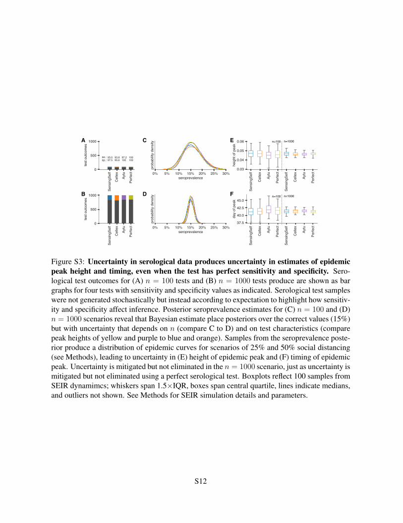
Figure S3: Uncertainty in serological data produces uncertainty in estimates of epidemicpeak height and timing, even when the test has perfect sensitivity and specificity. Sero-logical test outcomes for (A) n = 100 tests and (B) n = 1000 tests produce are shown as bargraphs for four tests with sensitivity and specificity values as indicated. Serological test sampleswere not generated stochastically but instead according to expectation to highlight how sensitiv-ity and specificity affect inference. Posterior seroprevalence estimates for (C) n = 100 and (D)n = 1000 scenarios reveal that Bayesian estimate place posteriors over the correct values (15%)but with uncertainty that depends on n (compare C to D) and on test characteristics (comparepeak heights of yellow and purple to blue and orange). Samples from the seroprevalence poste-rior produce a distribution of epidemic curves for scenarios of 25% and 50% social distancing(see Methods), leading to uncertainty in (E) height of epidemic peak and (F) timing of epidemicpeak. Uncertainty is mitigated but not eliminated in the n = 1000 scenario, just as uncertainty ismitigated but not eliminated using a perfect serological test. Boxplots reflect 100 samples fromSEIR dynamimcs; whiskers span 1.5×IQR, boxes span central quartile, lines indicate medians,and outliers not shown. See Methods for SEIR simulation details and parameters.

S12

0 5000 10000 150000.5

0.6

0.7

0.8

0.9

1.0

90\%

CI c

over

age

(ove

rall

sero

prev

.)

5%

10%

15%20%25%

30%

Newborn blood spots93.0% sensitivity97.5% specificity

0 5000 10000 150000.5

0.6

0.7

0.8

0.9

1.0

5%10%15%

20%

25%30%

U.S. blood donors93.0% sensitivity97.5% specificity

0 5000 10000 150000.5

0.6

0.7

0.8

0.9

1.0

5%10%15%20%25%30%

Model & Demog. Informed93.0% sensitivity97.5% specificity

0 5000 10000 150000.5

0.6

0.7

0.8

0.9

1.0

5%10%

15%

20%

25%30%

Uniform93.0% sensitivity97.5% specificity

0 5000 10000 150000.5

0.6

0.7

0.8

0.9

1.0

90\%

CI c

over

age

(ove

rall

sero

prev

.)

5%

10%15%

20%25%30%


0 5000 10000 150000.5

0.6

0.7

0.8

0.9

1.0

5%

10%15%

20%

25%30%


0 5000 10000 150000.5

0.6

0.7

0.8

0.9

1.0

5%10%

15%20%25%

30%


0 5000 10000 150000.5

0.6

0.7

0.8

0.9

1.0

5%

10%15%20%25%

30%


0 5000 10000 150000.5

0.6

0.7

0.8

0.9

1.0

90\%

CI c

over

age

(ove

rall

sero

prev

.)

5%

10%

15%

20%25%30%

Newborn blood spots97.2% sensitivity100% specificity

0 5000 10000 150000.5

0.6

0.7

0.8

0.9

1.0

5%

10%15%20%

25%

30%

U.S. blood donors97.2% sensitivity100% specificity

0 5000 10000 150000.5

0.6

0.7

0.8

0.9

1.0

5%10%15%

20%25%30%

Model & Demog. Informed97.2% sensitivity100% specificity

0 5000 10000 150000.5

0.6

0.7

0.8

0.9

1.0

5%

10%15%20%

25%

30%

Uniform97.2% sensitivity100% specificity

0 5000 10000 15000samples (n)

0.5

0.6

0.7

0.8

0.9

1.0

90\%

CI c

over

age

(ove

rall

sero

prev

.)

5%

10%

15%20%25%

30%

Newborn blood spots100% sensitivity100% specificity

0 5000 10000 15000samples (n)

0.5

0.6

0.7

0.8

0.9

1.0

5%10%

15%20%25%

30%

U.S. blood donors100% sensitivity100% specificity

0 5000 10000 15000samples (n)

0.5

0.6

0.7

0.8

0.9

1.0

5%10%15%20%25%30%

Model & Demog. Informed100% sensitivity100% specificity

0 5000 10000 15000samples (n)

0.5

0.6

0.7

0.8

0.9

1.0

5%10%15%20%

25%30%

Uniform100% sensitivity100% specificity

Overall seroprevalence estimation

Figure S4: Credible interval coverage for overall seroprevalence estimates using four sam-pling strategies and four serological test kits. Credible interval coverage, defined as the frac-tion of posterior credible intervals that covered the true parameter used to generate the data, areshown for four sampling strategies (columns, colors) and four test kits (rows), with sensitivityand specificity values as indicated; see legends. Each point represents the fraction of credibleintervals which covered the planted value for the indicated overall seroprevalence value (seeannotations on plots) at the specified number of serological samples n, out of a total of 250independent trials. The estimated coverage from a perfectly calibrated posterior will have cov-erage fractions within 0.9 ± 0.37 (grey bands) 95% of the time. Some seroprevalence valuesare plotted in black simply to guide the eye. The MDI strategy shown was designed to optimizeestimation of Reff.

S13

0 5000 10000 15000

0.01

0.02

0.03

0.04

0.05

0.06

0.07

0.0890

\% C

I wid

th (o

vera

ll se

ropr

eval

ence

)

5%

10%

15%

20%25%30%


0 5000 10000 15000

0.01

0.02

0.03

0.04

0.05

0.06

0.07

0.08

5%

10%

15%20%25%30%


0 5000 10000 15000

0.01

0.02

0.03

0.04

0.05

0.06

0.07

0.08

5%

10%

15%20%25%30%


0 5000 10000 15000

0.01

0.02

0.03

0.04

0.05

0.06

0.07

0.08

5%

10%

15%20%25%30%


0 5000 10000 15000

0.01

0.02

0.03

0.04

0.05

0.06

0.07

0.08

90\%

CI w

idth

(ove

rall

sero

prev

alen

ce)

5%

10%

15%20%25%30%


0 5000 10000 15000

0.01

0.02

0.03

0.04

0.05

0.06

0.07

0.08

5%

10%15%20%25%30%


0 5000 10000 15000

0.01

0.02

0.03

0.04

0.05

0.06

0.07

0.08

5%

10%15%20%25%30%


0 5000 10000 15000

0.01

0.02

0.03

0.04

0.05

0.06

0.07

0.08

5%

10%15%20%25%30%


0 5000 10000 15000

0.01

0.02

0.03

0.04

0.05

0.06

0.07

0.08

90\%

CI w

idth

(ove

rall

sero

prev

alen

ce)

5%

10%

15%

20%25%30%


0 5000 10000 15000

0.01

0.02

0.03

0.04

0.05

0.06

0.07

0.08

5%

10%

15%20%25%30%


0 5000 10000 15000

0.01

0.02

0.03

0.04

0.05

0.06

0.07

0.08

5%

10%

15%20%25%30%


0 5000 10000 15000

0.01

0.02

0.03

0.04

0.05

0.06

0.07

0.08

5%

10%

15%20%25%30%


0 5000 10000 15000samples (n)

0.01

0.02

0.03

0.04

0.05

0.06

0.07

0.08

90\%

CI w

idth

(ove

rall

sero

prev

alen

ce)

5%

10%

15%

20%25%30%


0 5000 10000 15000samples (n)

0.01

0.02

0.03

0.04

0.05

0.06

0.07

0.08

5%

10%

15%20%25%30%


0 5000 10000 15000samples (n)

0.01

0.02

0.03

0.04

0.05

0.06

0.07

0.08

5%

10%

15%20%25%30%


0 5000 10000 15000samples (n)

0.01

0.02

0.03

0.04

0.05

0.06

0.07

0.08

5%

10%

15%20%25%30%


Figure S5: Average credible interval width for overall seroprevalence estimates using foursampling strategies and four serological test kits. Credible intervals were calculated for datagenerated according to four sampling strategies (columns, colors) and four test kits (rows), withsensitivity and specificity values as indicated; see legends. Each point represents the averagewidth of the intervals for the indicated overall seroprevalence value (see annotations on plots)at the specified number of serological samples n, out of a total of 250 independent trials. Someseroprevalence values are plotted in black simply to guide the eye. The MDI strategy shown wasdesigned to optimize estimation of Reff. Sampling strategies that resulted in posterior credibleintervals with inaccurate coverage (see Supplementary Fig. S4) are crossed out.

S14

0 5000 10000 150000.5

0.6

0.7

0.8

0.9

1.0

90\%

CI c

over

age

(Reff)

5%

10%15%20%25%

30%


0 5000 10000 150000.5

0.6

0.7

0.8

0.9

1.0

5%10%15%20%25%30%


0 5000 10000 150000.5

0.6

0.7

0.8

0.9

1.0

5%

10%15%

20%25%

30%


0 5000 10000 150000.5

0.6

0.7

0.8

0.9

1.0

5%

10%

15%20%25%30%


0 5000 10000 150000.5

0.6

0.7

0.8

0.9

1.0

90\%

CI c

over

age

(Reff) 5%

10%15%

20%

25%30%


0 5000 10000 150000.5

0.6

0.7

0.8

0.9

1.0

5%10%15%20%25%

30%


0 5000 10000 150000.5

0.6

0.7

0.8

0.9

1.0

5%10%15%

20%25%30%


0 5000 10000 150000.5

0.6

0.7

0.8

0.9

1.0

5%

10%15%20%25%30%


0 5000 10000 150000.5

0.6

0.7

0.8

0.9

1.0

90\%

CI c

over

age

(Reff)

5%

10%15%

20%

25%30%


0 5000 10000 150000.5

0.6

0.7

0.8

0.9

1.0

5%10%15%20%25%30%


0 5000 10000 150000.5

0.6

0.7

0.8

0.9

1.0

5%10%

15%20%

25%

30%


0 5000 10000 150000.5

0.6

0.7

0.8

0.9

1.0

5%10%

15%20%25%

30%


0 5000 10000 15000samples (n)

0.5

0.6

0.7

0.8

0.9

1.0

90\%

CI c

over

age

(Reff)

5%

10%15%20%

25%30%


0 5000 10000 15000samples (n)

0.5

0.6

0.7

0.8

0.9

1.0

5%

10%15%20%

25%

30%


0 5000 10000 15000samples (n)

0.5

0.6

0.7

0.8

0.9

1.0

5%10%

15%

20%25%30%


0 5000 10000 15000samples (n)

0.5

0.6

0.7

0.8

0.9

1.0

5%

10%

15%20%25%30%


Reff estimation

Figure S6: Credible interval coverage for Reff estimates using four sampling strategiesand four serological test kits. Credible interval coverage, defined as the fraction of posteriorcredible intervals that covered the true parameter used to generate the data, are shown for foursampling strategies (columns, colors) and four test kits (rows), with sensitivity and specificityvalues as indicated; see legends. Each point represents the fraction of credible intervals whichcovered the planted value for the indicated overall seroprevalence value (see annotations onplots) at the specified number of serological samples n, out of a total of 250 independent trials.The estimated coverage from a perfectly calibrated posterior will have coverage fractions within0.9±0.37 (grey bands) 95% of the time. Some seroprevalence values are plotted in black simplyto guide the eye. The MDI strategy shown was designed to optimize estimation of Reff.

S15

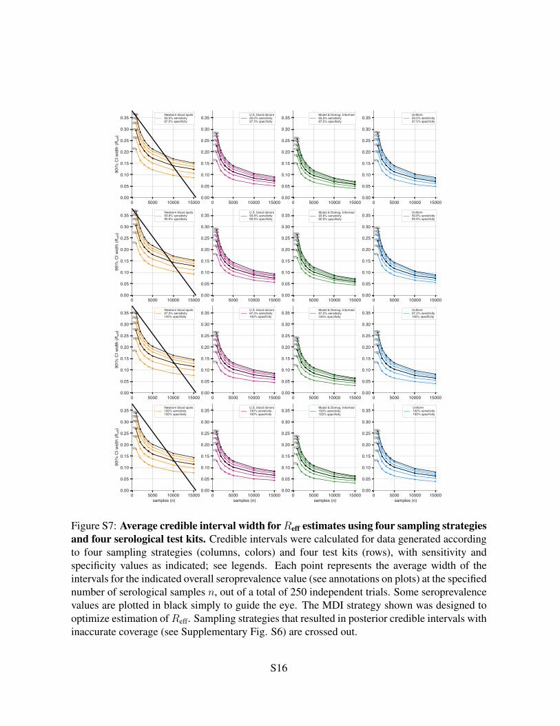
0 5000 10000 150000.00

0.05

0.10

0.15

0.20

0.25

0.30

0.3590

\% C

I wid

th (R

eff)

5%

10%

15%

20%25%30% Newborn blood spots


0 5000 10000 150000.00

0.05

0.10

0.15

0.20

0.25

0.30

0.35

5%

10%

15%20%25%30%


0 5000 10000 150000.00

0.05

0.10

0.15

0.20

0.25

0.30

0.35

5%

10%

15%20%25%30%


0 5000 10000 150000.00

0.05

0.10

0.15

0.20

0.25

0.30

0.35

5%

10%

15%

20%25%30%


0 5000 10000 150000.00

0.05

0.10

0.15

0.20

0.25

0.30

0.35

90\%

CI w

idth

(Ref

f)

5%

10%

15%

20%25%30% Newborn blood spots


0 5000 10000 150000.00

0.05

0.10

0.15

0.20

0.25

0.30

0.35

5%

10%

15%20%25%30%


0 5000 10000 150000.00

0.05

0.10

0.15

0.20

0.25

0.30

0.35

5%

10%

15%20%25%30%


0 5000 10000 150000.00

0.05

0.10

0.15

0.20

0.25

0.30

0.35

5%

10%

15%20%25%30%


0 5000 10000 150000.00

0.05

0.10

0.15

0.20

0.25

0.30

0.35

90\%

CI w

idth

(Ref

f)

5%

10%

15%

20%25%30%


0 5000 10000 150000.00

0.05

0.10

0.15

0.20

0.25

0.30

0.35

5%

10%

15%20%25%30%


0 5000 10000 150000.00

0.05

0.10

0.15

0.20

0.25

0.30

0.35

5%

10%

15%20%25%30%


0 5000 10000 150000.00

0.05

0.10

0.15

0.20

0.25

0.30

0.35

5%

10%

15%20%25%30%


0 5000 10000 15000samples (n)

0.00

0.05

0.10

0.15

0.20

0.25

0.30

0.35

90\%

CI w

idth

(Ref

f)

5%

10%

15%

20%25%30%


0 5000 10000 15000samples (n)

0.00

0.05

0.10

0.15

0.20

0.25

0.30

0.35

5%

10%

15%20%25%30%


0 5000 10000 15000samples (n)

0.00

0.05

0.10

0.15

0.20

0.25

0.30

0.35

5%

10%

15%20%25%30%


0 5000 10000 15000samples (n)

0.00

0.05

0.10

0.15

0.20

0.25

0.30

0.35

5%

10%

15%20%25%30%


Figure S7: Average credible interval width forReff estimates using four sampling strategiesand four serological test kits. Credible intervals were calculated for data generated accordingto four sampling strategies (columns, colors) and four test kits (rows), with sensitivity andspecificity values as indicated; see legends. Each point represents the average width of theintervals for the indicated overall seroprevalence value (see annotations on plots) at the specifiednumber of serological samples n, out of a total of 250 independent trials. Some seroprevalencevalues are plotted in black simply to guide the eye. The MDI strategy shown was designed tooptimize estimation ofReff. Sampling strategies that resulted in posterior credible intervals withinaccurate coverage (see Supplementary Fig. S6) are crossed out.

S16

Supplementary Tables

Manufacturer Type of Test Sens. Spec. Sales Approval∗Sensing Self IgG 93 97.5 CESensing Self IgM 82 96 CE†Cellex Inc. IgM & IgG 93.8 95.6 FDA, CE†Aytu Biosciences/Orient Gene Biotech IgG 97.2 100 CE, ChinaAytu Biosciences/Orient Gene Biotech IgM 87.9 100 CE, ChinaScanWell Health/INNOVITA IgM & IgG 87.3 100 ChinaSD Biosensor IgM & IgG 82 97 KoreaLiming Bio IgG 82 100 CE, IVDLiming Bio IgM 62 100 CE, IVDShenzhen Yhlo Biotech Company IgG 90 95 CE, IVDShenzhen Yhlo Biotech Company IgM 95 95 CE, IVD∗ included only in main text modeling, calculations, and figures.† included in Supplementary modeling, calculations, and figures.1 http://www.centerforhealthsecurity.org/resources/COVID-19/serology/Serology-based-tests-for-COVID-19.html

Table S1: Serological tests used in this study. Sensitivity and specificity values were takenfrom manufacturer’s claims as of April 9, 2020, compiled by the Johns Hopkins Center forHealth Security1.

S17

Parameter Meaning Value Referenceα transition rate E → I 0.2β infectiousness 1.75γ recovery rate 0.5ρ social distancing effects 0.5, 0.75θ seropositive fraction various see Methodsui Susceptibility of age group i 0.078 (10)

yiProbability that an infection is clinical

for an age-i individual

[0.056, 0.056, 0.056, 0.064,0.100, 0.162, 0.240, 0.322,0.398, 0.455, 0.486, 0.535,

0.723, 0.740 , 0.740 , 0.740]

(10)(see caption)

CijNumber of age-j individuals contacted by

an age-i individual per dayvarious

(8)(see caption)

µp Mean duration of preclinical infectiousness 2.4 days (10, 26)µc Mean duration of clinical infectiousness 3.2 days (10, 27)µs Mean duration of subclinical infectiousness 7 days (10)f Relative infectiousness of subclinical cases 50% (10)

θi Seropositivity of age-i subpopulation

θ + [-0.014, -0.012, -0.004, 0.002,0.008, 0.015, 0.018, 0.020,0.006, 0.005, 0.003, -0.003,

-0.009, -0.010, -0.012, -0.012],with various θ, representingthe average seroprevalence

Table S2: Parameter values used in models. This table is divided into two sections. The topsection corresponds to the parameters of the single-population SEIR model. The bottom sectioncorresponds to the parameters used in the age-structured SEIR model. Contact matrices Cijused in this manuscript were, in particular, those corresponding to the United States of Americaand India. Values for yi, the probability that an infection is clinical for an age-i individual,were generated by using three control points for young, middle and old age, then interpolatingbetween them with a cosine-smoothing function, as described in (10). Equations for modelscan be found in Supplementary Text. Test kit sensitivity and specificity values are provided inSupplementary Table S1.

S18

seroprevalence with uncertainty - dash home

Documents