7 DA~ 4 R FESTSCHRIFT'OF TECHNICL PPERS PRESENTED TO WILHELM i/iRD-R4l 48 SERICKSEN ON THE..(U) AIR FORCE INST OF TECH

NRIGHT-PATTERSON AF8 OH B W4 WOODRUFF JAN 84NC4SFE FTEN-TM-84-i F/G 5/2 N

Ir .t,,.. ,., ,,,.,. . ., ,_- .- . -. . . . . .. , . -. . . . .. .. .. , -C .-.- ,,t. -,. - . ,,. . .. -. -.,. -, . ,

/ 'f

u.,.s.U.0

w..L3.

MICROCOPY RESOLUTION TEST CHART

M Y

mil

"'Si

lbS is*41 .:':.;-7,--;',. ;-': :" -:-;- ."". --. . .', - .. .- -.. . . .":

' i -' o . ,," 'I F ? v ' ..'..")"-, ,' ..% .' : w ','w,-.%.-'-:,'.',.;,'-,.. :-,.% -.;..".' -'.,'.,-. %.," ,_.,. ,,. ,p

'f I l i l I | ,~ 128 ,,, ". . r. , " . ,

-. 17

A FESTSCHRIFT OF TECHNICAL PAPERSPRESENTED TO WILHELM S. ERICKSEN

ON THE OCCASION OF HIS JOINING

THE EMERITUS FACULTY OF THE

AIR FORCE INSTITUTE OF TECHNOLOGY

AFIT-EN-TM-84-1 Brian W. Woodruff

Captain USAFEditor

.4 $ MY24/

4%*A

0A

I.'.

%.°,. .

KUproved foT public meleaNt lAW AFR 190-]17.

LYNN E. WOLAVER Dean for Research and ProfesIonal DevlopmentAir Force Institute of EchNOLOg A).

A.Wright.Pattson Br.i .4Wod

84 05 23 025

SE . ' - , WOA W ..-

Foreword

Wilhelm Schelstadt Ericksen earned the Bachelor of Arts inMathematics at St. Olaf College in 1936. He earned the Master ofArts in Mathematics dt the University of Wisconsin in 1938. He was

dissertation on, "Asyrmptotic Forris o the Solutiots of theDifferential Equation for the Associated Mathieu Functions."

He began his college teaching career in 1942 at St. Olaf-. College, and he taught at Minot State Teachers' College for the

academic year 1943-44. He was a Fellow in Mechanics at BrownUniversity in 1944-45.

Dr. Ericksen worked as an aerodynamicist for Bell Aircraftin14.and in that year he also began a six-year association with

the United States Forest Products Laboratory in Madison, Wiscon-sin. He joined the faculty of the United States Air Force Instituteof Technology in 1953.series Professor Ericksen's long list of publications began with a

4. series of Forest Products Laboratory reports on the behavior of,:' sandwich panels under loads, and continues with recent articles in

the Society for Industrial and Applied Mathematics' Journal on Nu-merical Analysis. on inverse pairs of matrices with integer ele-ments.

Wilhelm Ericksen's teaching is characterized by scholar-ship of the highest degree, coupled with a caring and gentle con-

" cern for his students as human beings. These splendid qualitieshave endeared him to thirty academic generations of AFIT studentsand to his colleagues, who present these papers to him as tokens oftheir affection and esteem on the occasion of his joining the emer-itus faculty.

,

K

'pp

' -"D. A. Lee -...... .. _ ___ __

-"*December 1982 3 -rlxt~AVailabIlity lodes

lAvati ai/or

SI' Sp'oc tu.

'Pt

TABLE OF CONTENTS,

The PCT Control System Design for Sampled-Data Control

Systems . . . .................... C. H. Houpis 1

' Asymptotic Non-Null Distribution of a Test of Equality of

Exponential Populations ..... R. W. Kulp and B. N. Nagarsenker . . . 17

-- Irrotational and Solenoidal Waves in General

Coordinates ........... .................... . D. A. Lee . . . 24

Some Problems of Estimation When Some Prior Information is

Available ......... ...................... . A. H. Moore . . . 29

Non-Null Distributions of the Likelihood Ratio Criterion for

the Spectral Matrix of a Gaussian Multivariate Time

Series ... ........................ .B. N. Nagarsenker . . . 41

Probability of Destruction of a Point Target in

Space .................... J. S. Przemieniecki . . . 53

A New Variational Principle for Elastodynamic Problems

p. with Mixed Boundary Conditions 19 t' C) . ...... ... P. J. Torvik . . . 59

' - The Validity of Linear Velocity Calculations of Low Pressure Gas

Flows in a Flow Tube . . . P. J. Wolf, E. A. Dorko and S. J. Davis . . . 70

iii

THE PCT CONTROL SYSTEM DESIGN FOR SAMPLED-DATA CONTROL SYSTEMS

*" -by

C. H. Houpis*

October 4, 1982

ABSTRACT

The pseudo-continuous-time (PCT) control system approximation of a sampled-

I. data system permits the use of tried and proven continuous-time domain methods

for designing cascade and/or feedback controllers. When the rules governing

the use of the Pade approximation and the Tustin transformation are satisfied,

the PCT design approach is a valuable technique for the design of sampled-data

control systems.

*Professor of Electrical Engineering, School of Engineering,Air Force Institute of Technology, Wriqht-Patterson AFB, Ohio 45433

4

* v, W @ . . . ..~ ~ ~ ... . - * '%'*'V*- " W ** *' * .'' ' -*' , L -- . ..

,,77.

I. Introduction

The analysis and design of sampled-data control systems may be done entirely

in the z-plane, which is referred to as the direct digital control design (DIR)

[21technique or entirely in the s-plane. The latter is referred to as the

digitization (DIG) technique which requires the development of the pseudo-

,-ontinuous-time (PCT) system model. This model requires the use of the Pade

and Tustin transformation approximations. A controllerD (z) designed by the DIG

technique provides a good base for exhibiting the effects of the sample time

]arameter of the digitized controller on the performance of the system. The

reason for this is that the continuous controller corresponds to the limiting

case where the sampling time of Dc (z) is zero. A disadvantage of this method

is that D (z) may not have all the properties of 0 (s). However, this problemC c

is minimized by the selection of a s to z (to w) transformation algorithm which

maintains the specified properties required of the controller. This paper

develops the PCT control system model and the criteria for achieving a good

correlation between the s- and z-plane mapping. If the degree of correlation

is not satisfactory, then the DIG technique may permit the desired system

performance characteristics to be achieved by mere gain adjustment in the

?-domain.

It. Approximations

ustin -- The Tustin s to z or z to s transformation is defined as'-.

S z (1)T T)l

or

Z +sT/2 (2)

and the exact z-transformation is defined as

Z -sT (3)

2

,5 By substituting s = Jsp into (21 and s - J sp into (3), where wsp

equivalent s-plane frequency, then equating the two expressiors results in

"' tan(, sp T/2) -- sp T/2 (4)

When W sp T/2 < 0.3057 rad 017o) then

"W' "sp W sp (5)P

In a similar manner, substituting the exponentional series for z = and

S s a sp into (2) results in

; sp T)2

I + ; sp T + P 2 +. + [YspT/(1-a so T/2)] (6)

If,' 1l >> 1 spT2 andlI >> I a pT2, then

(;pl=l~l<< 2/T (7)

~With (5) and (7) satisfied, the shaded area in Fig. I represents the allowable

" location of the poles and zeros in the s-plane for a good Tustin transformation.

wQ.,-Pade -- Using the first-order Pade approximation, the transfer function of

the zero-order-hold (Z-O-H) device is approximated~when the value of T is small

'44

,:' enough 4 , as follows:

. -Ts.Gzo(S s 1 T =+_ G pa(s ) (8)

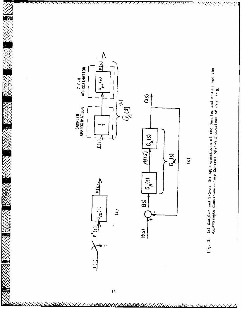
), 111. Pseudo Continuous-Time Control System (PCTaThe DIG method of designing a saled-data system, in the complex frequency

s-plane, requires a satisfactory PCT model of the sampled-data system. In other

words, for the sampled-data system of Fig. 2, the sampler and the Z-O-H units

are approximated by a linear continuous-time unit, GA(s), as shown in Fig. 3(c).

The DIG method requires that the dominant poles and zeros of the PCT model

% must lie in the shaded area of Fig or a high level of correlation with

1,- -; .',,; T- -.. 1 " -,,-. T( . (6)-....... ...

sp. .. .. sp ' ,., -', - , .: -.:T'" .:,-',': ,..." ? ,

the sampled-data system. To determine GA(S) first note that the frequency

component of E*(jw), representing the continuous-time signal E(jw) and all of

its side-bands, is multiplied by lI/T [1,2. Because of the low-pass filtering

characteristics of a sampled-data system, only the primary component needs to

be considered in the analysis of the system. Therefore, the PCT approximation

of the sampler and the Z-O-H of Fig. 3(a) is shown in Fig. 3(b) where the Pade

approximation, Gpa(s), is used to replace Gzo(s). Therefore, the sampler and

Z-O-H units of a sampled-data system are approximated in the PCT system of Fig.

3(c) by the transfer function

GA )~G (s 2 --A(S) T paS = + + (9)

Since Lir [GA(s)] = 1, (9) is an accurate PCT representation of the sampler and

Z-Q-H units, satisfying the requirement that as T - 0 the output of GA(S) must

equal its input. Further note that in the frequency domain, as ws 4 + (T - 0),

,r. the primary strip in the s-plane becomes the entire frequency spectrum domain

which is the representation for the continuous-time system.

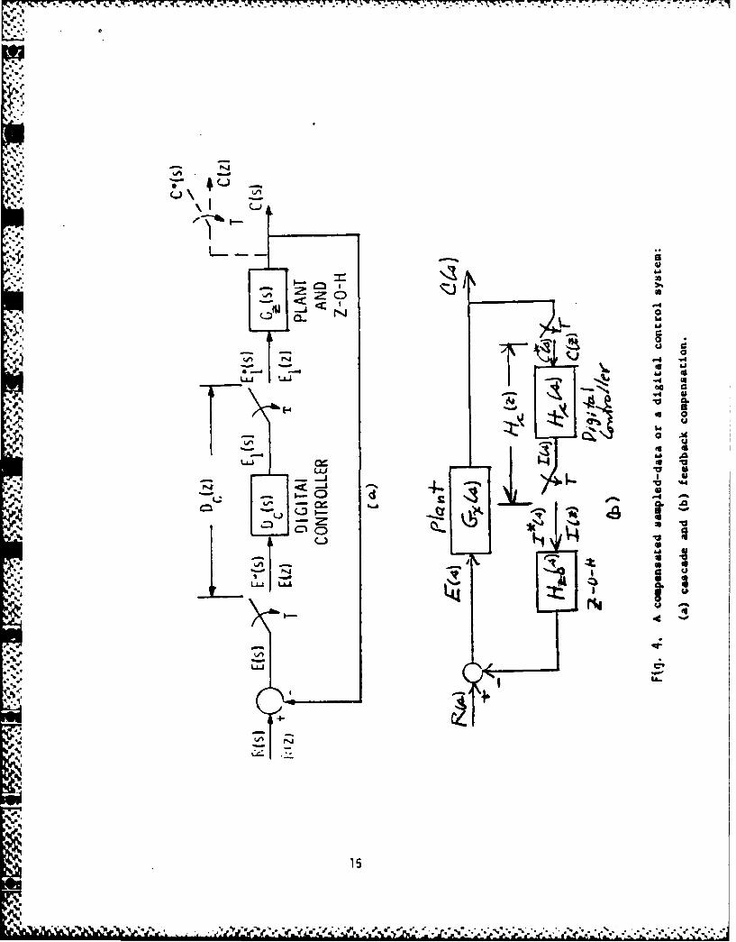
Note that in obtaining PCT systems for the sampled-data systems of Fig. 4,

the factor I/T replaces only the sampler that is sampling the continuous-time

ignal. The sampler on the output of the digital controller is replaced by a

factor of one. To illustrate the effect of the value of T on the validity of

the results obtained by the DIG method, consider the sampled-data closed-loop

control system of Fig. 2 where

G(S) 4.2x S S+l)(S+5)

The closed-loop system performance for three values of T and c 0.45 are

determined in both the s- and z- domains, i.e., the DIG and DIR methods,

respectively. Table I presents the required value of K and time response

characteristics for each value of T. Note that for T _ 0.1 there is a hiqh

,.

--- "wP* ~~ * ~

correlation between the DIG and DIR models. For T < 1 there is still a re-

latively good correlation. (The designer needs to specify, for a given

application, what is considered to be "good correlation.") The figures of

merit of the corresponding continuous-time control system

G(s)(10)A7 I'+Gx (s }

for a unit-step forcing function are: Mp 1.202, tp = 4.12 sec and ts = 9.48 sec.

Table I Performance Characteristics of a Sampled-data Control

System using the DIR and DIG Methods

Method T, sec K x M e t s sec

DIR 04.147 1.202 4.16 9.53,. ,DI R0.01

DIG 4.215 1.206 4.11 9.478

DIR 3.892 1.202 4.25 9.8k.'. 0.1

DIG 3.906 1.203 4.33" 9.90

DIR 2.4393 1.2 6 13+

DIG 2.496 1.200 6.18 13.76

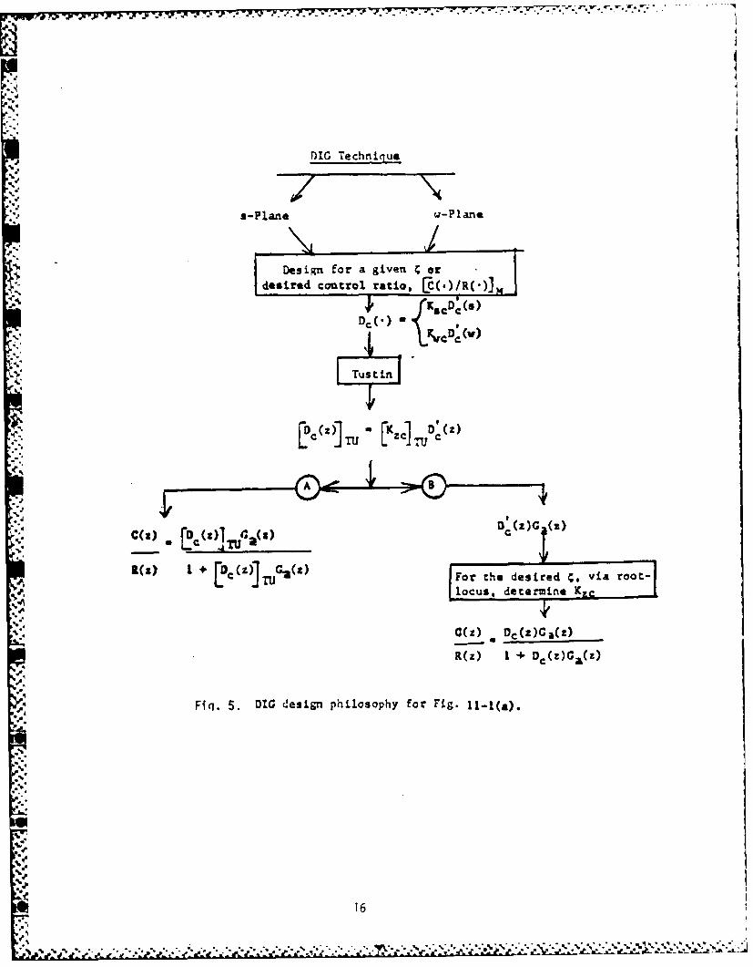
IV. DIG Technique

Figure 5 represents the trial and error design philosophy in applying the

DIG technique. If path A does not result in the specifications being met by

the sampled-data control system of Fig. 4, then path B is used to try to

determine a satisfactory value of Kzc. A similar chart may be drawn for the

design of the feedback controller of Fig. 4(b). The design philosophy involves

the following considerations:

(a) Follow path A if the dominant poles and zeros of C(.)/R(.) lie in the

shaded area of Fig. 1 (Tustin approximation is good).

(b) Follow path A when the degree of warping is deemed not to negatively

affect the achievement of the desired design results. If the desired results

are not achieved try path B.

5

(c) Follovw path B when severe warping exists. The DIG design procedure

is as follows:

Step 1 Convert the basic sampled-data control system to a PCT control

system or transform the basic system Into the w-plane (use both for design

ourposes).

Step 2 By means of a root-locus analysis or by use of the Guilleman-

Truxal method determine Dc -s- KscDcCS) or Dc (w) = KwsDc(W).

Step 3 Obtain the control ratio of the compensated system and the corre-

sponding time response for the desired forcing function. (This step is not

necessary if the exact Guillemin-Truxal compensator is used.) If the desired

performance results are not achieved, repeat Step 2 by selecting a different

value of c, as wd' etc. or a different desired control ratio.

Step 4 When an acceptable D Csy or Dc w) has been achieved, transform

the compensator, via the Tusttn transformation, into the z-domain.

Step 5 Obtain the z-domatn control ratio of the compensated system and

the corresponding time response for the desired forcing function. If the

desired performance results for the sampled-data control system are

achieved via path A or path B, then the design of the compensator is complete.

If not, return to Step 2 and repeat the steps with a new compensator design

or proceed to the DIR technique.

V. DIR Technique

The simple lead (a < 1) and lag (a > 1) compensators in the s-domain have

the form

K sc-(s z S)c((s) s s 1ps)

where ps Zs/'I. The s-plane zero and pole are transformed into the z-domain

as follows:

4 6'4,C..

"'-'4 ""€ .2 '' , :2 ,. " " .. ,:'.' : Y, -:. ,..,:'-' "" '" . ' . . ."" .. . .

.4...- -. -

sT z sT

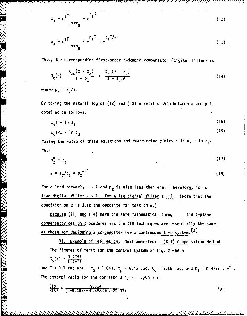
zz -- T (12)s=zs

sT - pT~ z T/a (3

Iz= S=P s 13

Thus, the corresponding first-order z-domain compensator (digital filter) is

D (Z) = K zc - zZ) KzcZ - zz)z Pz z - Z (14)

C Z -p z/

where pz = z/S.

By taking the natural log of (12) and (13) a relationship between a and s is

obtained as follows:

ZsT = In (15)

zsT/a = In P(16)

Taking the ratio of these equations and rearranging yields a In nz = In zZ '

Thus

P z(17)z z

a = Zz/P z = pz.-l (18)

For a lead network, a < 1 and pz is also less than one. Therefore, for a

lead digital filter a > 1. For a lag digital filter s < 1. (Note that the4.

condition on 8 is just the opposite for that on a.)

Because (11) and (14) have the same mathematical form, the z-plane

compensator design procedures via the DIR techniques are essentially the same

as those for designing a compensator for a continuous-time system. [ 3]

V[. Example of DIG Design: Guillaman-Truxal (G-T) Compensation Method

The figures of merit for the control system of Fig. 2 where

G(S) =0.4767x s(s+l)

and T = 0.1 sec are: MP = 1.043, tp = 6.45 sec, ts = 8.65 sec, and KI 0.4765 sec-

The control ratio for the corresponding PCT system is

C~)9.534

= (s+O. 4875+jO. 4883)(s'20.0J) (19)

7

*% ."-

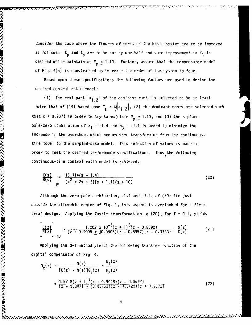
Consider the case where the figures of merit of the basic system are to be improved

as follows: tp and ts are to be cut by one-half and some improvement in K1 is

ppdesired while maintaining Mp< 1.10. Further, assume that the compensator model

of Fiq. 4(a) is constrained to increase the order of the.system to four.

Based upon these specifications the following factors are used to derive the

desired control ratio model:

(1) The real part Icl,2 1 of the dominant roots is selected to be at least

twice that of (lQ) based upon Ts 2 4/1 1 , 2 1 , (2) the dominant roots are selected such •

that c = 0.7071 in order to try to maintain M < 1.10, and (3) the s-plane Np

pole-zero combination of z1 = -1.4 and P3 = -1.1 is added to minimize the

increase in the overshoot which occurs when transforming from the continuous-

time model to the sampled-data model. This selection of values is made in

order to meet the desired performance specifications. Thus the following

continuous-time control ratio model Is achieved.

= 15.714(s + 1.4) (20)

M (s + 2s + 2)(s + 1.1)(s + 10)

Although the zero-pole combination, -1.4 and -1.1, of (20) lie just

outside the allowable region of Fig. 1, this aspect is overlooked for a first

trial design. Applying the Tustin transformation to (20), for T = 0.1, yields

C~z 7.202 x (03(z + 1) oK (1IN KkZ) (z - 0.9005 + J0.0905)(z - 0.8957)(z - 0.3333) D(z (21)J- -U

Applying the G-T method yields the following transfer function of the

digital compensator of Fig. 4.

cZ _D~ - N(z) ( El(z)

DE 2(z)[D(z) - N(z)]G z(z) E2 (z)

0.5218(z + 1) 3(z - 0.9048)(z - 0.3692)(z - 0.8471 + jO.03753)(z -").342 )(z - 0.9672)

9.?

.

" Note, that as a consequence of the use of the G-T method and the Tustin approximation,

the order of the numerator of Dc (z) is greater than the order of the denominator

by one.

A practical approach to achieving a physically realizable Dc(z) is to

replace one of the (z + 1) factors which appear as a result of the Tustin

transformation, by its d-c gain factor [2] of (z + l)lz~ = 2 in the numerator

of 0 c(z) to yield

D K zc (Z + l)2 (z - 0.9048)(z - 0.86921)

c(z) : (z - 0.8471 + jO.03753)(z - 0.3420)(z + 0.9672) (23)

where Kzc 2(0.5218) = 1.0436. With this controller, the control system'sS-l

figures of merit are: Mp = 1.031, tp Z 3.55 sec, ts = 4.25 sec, and KI = 0.77193 sec

The specific value of t < 6.45/2 can be met by increasing the value of Kzcp z

to 1.14918.

As illustrated by this example a physically unrealizable controller may result

when applying the Guillemin-Truxal inethod to [C(z)/R(z)]TU. In order to maintain

the d-c gain and achieve a physically realizable controller, one approach, asapplied to this example, is to replace one or more (z + 1) numerator factors

of 0 c(z) by the d-c gain factor of 2.

VII. Conclusions

By the use of the Pade approximation and the Tustin transformation, a

sampled-data control system may be transformed into a PCT control system. As

the examples illustrate, when the rules governing this transformation are

satisfied the analysis and design of a PCT system model is a practical approach

for the analysis and design of a sampled-data control system. The standard

first-order z-plane compensator, K ZC(z-zz)/(Z-z /3), corresponds to the standard

first-order s-plane compensator, K SC(s-zs)/(S-zs/) where for a lead compensator

9

° - o o ° . .

LIt

3 < I and : > 1. A consequence of applying the Tustin transformation to

C(s)/R(s) of the PCT system and then applying the fl-T method to [C(z)/R(z)]TU

is that an unrealizable cascade digital comnensator Dc(Z) results. This paper

illustrates a method by which this Dc(z) may be made realizable by replacing

one or more (z+l) factor in the numerator, due to the Tustin transformation,

by its d-c qain factor of two.

-'.

,. .

". 1.1 Oppenheim, A. V. and R. W. Schafer "Digital Signal Processing," Prentice-

Hall, Englewood Cliffs, NJ, 19

2. Houpis, C. H. and G. B. Lamont "Digital Control System (Theory, Hardware,

Software)," McGraw-Hill Book Co., NY, NY, Fall, 1983.

3. D'Azzo, J. J. and C. H. Houpis "Linear Control Systems Analysis and Design:

Conventional and Modern," McGraw-Hill Book Co., NY, NY, 2nd Ed, 1981.

4. Wall, H. S. "Analytic Theory of Continued Fractions," D. Van Nostrand

Company, Inc., 1948.4.,

.d'. .'-

....

.o.

-

.:- ....

6'%'

" 2 .3.14

s-PLAINE

*4 I

•j .6 114/

--.-. 3.1t4

Z.' T'Fig. I Ulowable location (shaded area) of lominint poles

.. ' and zeros in :i-pla.ae for a Aucd rustin approximation.

12

, °

t ,3..4

";'p-, . :,','.:..'. :.r "; ', .' .," .. t: ' " "> 7.< z,,¢ :Y *: :.' "z,., ., .- .,_...,,, -, v " ---. .".."> -"."."""-,. ,

--.- n

p'...

'S,. I 4

-z- ,p y' w'w~~ -~ -y-~. - - - . -.

~-- 4

L~-4

*4* ,.

4,

4.

P

N

04

.4 .4 --- 4

4~4 4 LLJ~ -4210

-p.-. I (/2 4

U, IJi

4'.'. 0

.4.' C., 0/2

Id' 4J(/24.~ - 2

.4 4,. XL.

*4 - WI

C.,

- '04-

'I,.1 U, - ~.

C.,NJ~.l' in

-. 4 t*404~

C'

-A U-

4~pIq4

4 4. ..- 14-. ~

h.P 4

r *(~40

wi ~a VLAJ V

Lu LLA -

.9, ,-,~('%.J

'~ O..I*-

* 9 +

15~

DIG Technique

s-Plane tg-?lane

D~oinfor a given 4o[desredcontrol ratio, C()R-]

Dc() K D'(e)

C(S) !()d'C-2.(x)

I~) I + Dc ( zJ. ,jG-a(z) For the desired ~.via root

locus. determine Kzc

C(Z) DC(Z)Gb(z)

R(z) I + Dc(z)GaCz)

Fiq. 5. DIG design philosophy for Fig. 11-1(&).

.16

'-IN

ASYMPTOTIC NON-NULL DISTRIBUTION OF A TEST

OF EQUALITY OF EXPONENTIAL POPULATIONS

R. W. Kulp and B. N. Nagarsenker

Air Force Institute of Technology

*Wright-Patterson Air Force Base, Ohio

Key Words and Phrases: exponential populations; likelihood ratio criterion;

asymptotic non-null distribution; Chi-square distributions.

Abstract

In this paper asymptotic expansions of the non-null distribution of the

likelihood ratio criterion for testing the equality of several one parameter

exponential distributions are obtained under local alternatives. These expan-

sions are in terms of Chi-square distributions.

1. Introduction

Suppose that p samples are available and that the ith sample contains n

observations x j with mean xi (i = 1,2,... ,p; j = 1,2,...,n) and has been drawn

from an exponential distribution with probability density given by4.i

f(x) = a 1 exp (-x/o ) x > 0, a i > 0

a 0 otherwise (i=l,2,...,p)

A test of hypothesis H0 that the p samples have been randomly drawn from the

same population is equivalent to testing that the p exponential distributions

in (1.1) are identical. In other words, it is desired to test the hypothesis

HO 0 2 p

17

.44.Ih

3gainst the general alternatives. The likelihood ratio criterion for testing

H0 is given by

n p nL " = [- (x /x) (1.2)

where x is the mean of the combined sample. The null distribution of L has been

considered by Jain, Rathie and Shah (1975), Nagarsenker (1980), Nagarsenker

et al. (1982) while the non-null distribution has been discussed by Mathai (1979).

For further references see Johnson and Kotz (1970).

In this paper, we first obtain the non-null moments in terms of zonal

.,-.%, polynomials and then use these to obtain the asymptotic expansion of the dis-

tribution of -2(n-u) In L where u = (p+l)/6p (see Nagarsenker (1980)), under the

sequence of local alternatives (see Khatri and Srivastava (1974))

(i) I - qE- = P/m and (ii) I - q 1 = Q/m (1.3)

where E - diag (Cli2o... , p), m = n - u, 0 < q < o while P and Q are fixed

matrices as m tends to infinity.

2. Preliminaries. .%q

We need the following lemmas in the sequel.

Lemma 1. The non-null hth moment of X defined in (1.2) is given by

.. n .nhn)(nh+n) F(pn+k)"..h) nh 7(nh+n)P qlinI

E(:qn7 C (M1) (2.1)f(n) I K k!F(pnh+pn+k) K) 2~k=0 K

where M I q- , 0 <q < and E = diag (io 2 ,. .. , )

4' Proof. To obtain the hth moment of X, we shall essentially use the method

give. in Wilks (1946) and the fact that xi are independently distributed as

I-

gammas with parameters n and j /n, i - 1,2,...,p. For this consider the.

function 0(9) where

t'()- E [E IT If e 'ti-l

It can be easily shown that -J

.4

P(nh+n) 1/nnh] -Ol1-(nh+n)NO JZnI1e~ (2.2)

-Jwhere 81 = 8/np. Using the following identity (see Khatri and Srivastava (1971)),

o (nh+n) C (M)II-e lli- (n+nh) (1-6 ,)-p(nh+n)lql-(nh+n) I I k

-~k-O K (l-81 q) k!.1*,

where 0 < q < o and can be chosen such that the expansion in the series form is

valid, i.e., 1 and q are such that

l lq(ch maxE)_lI < (1-qal) 1

4h d r (9)E(A ) is then obtained by evaluating dr at 9 - 0 and then putting r - -nh

(see Wilks (1946) for the validity of such operation). This gives (2.1).

Remark. Taking q - a2, we get the null moments of X given in Nagarsenker (1980).

Lemma 2. Let C CZ) be a zonal polynomial corresponding to the partition

( kltk 2 ".. kp} with k1 + k2 + ... + k andk >k .k k _ 0. Let

1 2p 2 p

al(K) = ki(ki-i), a2(K) ki(4k 2 -6ik +32)

il i= i

and 0 - tr(Zr). Then the following equalities hold:r -

19

.4

a19 .

,.4,

-- -%4 - iv *.'+"i ' + 'r " " " ,. ," •

"+ - - " *- """ '" .' .'*. .- ,- - - .,' -- -_ -,,-

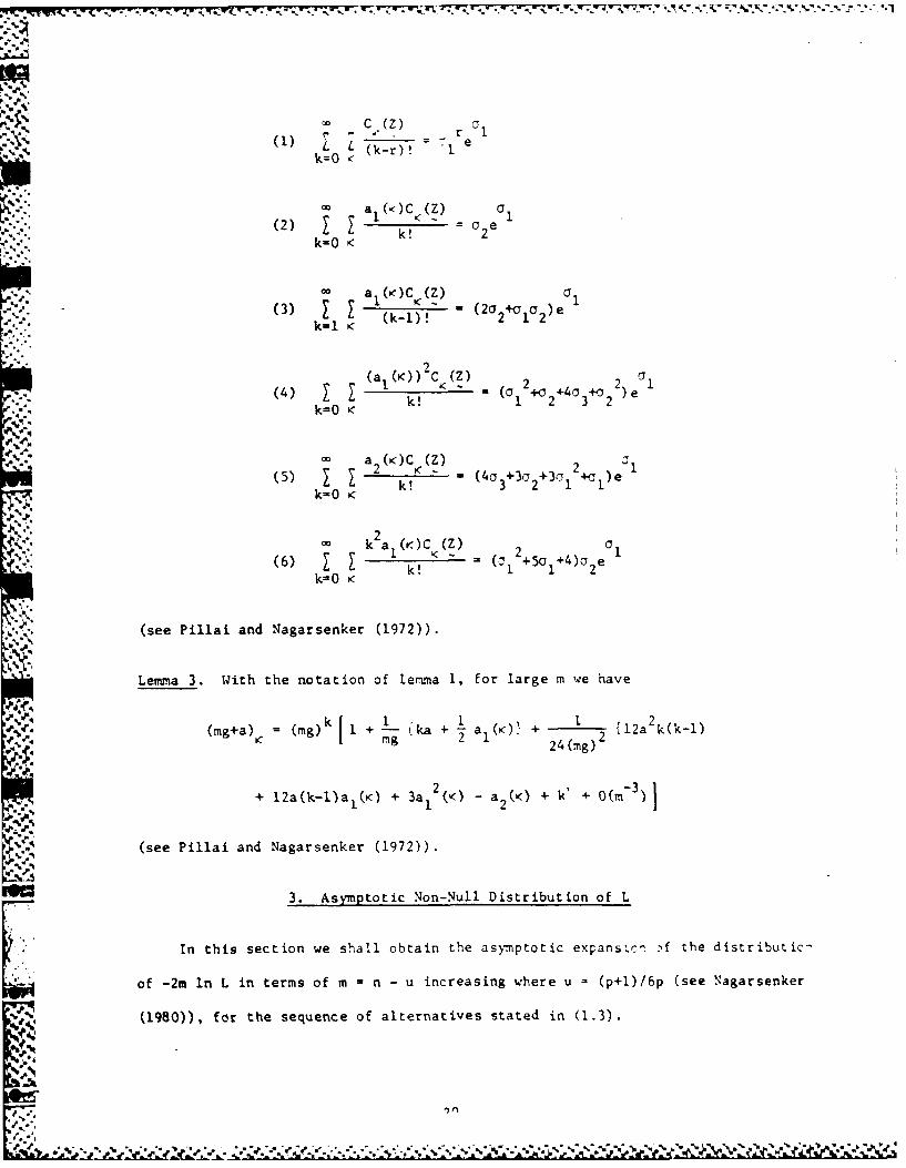
%-: 00 c Q) CT

7~- .- -, r

(L (k-r)' I

a (a)C ( )

(2) k 1 k! = ek=O K

(a (K))2C (Z) 2(4) 1 (a 2+0 +4"+0 2 e I

II k! 1 2 3 2

v,,.',k=l i

00 a 2 ( K)C (Z) 2 1(5) ~ 1 ,--- (4a +3(3+30 C

k3 2 1 1k=O K

k a (K)C (Z) 20

(6) k 1 +50 1+4) ek=0 K

(see Pillai and Nagarsenker (1972)).

Lemma 3. With the notation of lemma 1, for large m we have

k I kk-ll

(mg+a): = (mg) k I + -g + a+(K) +a, I12a 2 k(k-l)Mg 2 24(mg)2

+ 12a(k-I)aI (K) + 3 a 1 2 (<) - a2(K) + k' + O(m- 3

. ~ (see Pillai and Nagarsenker (1972)).

3. Asymptotic Non-Null Distribution of L

In this section we shall obtain the asymptotic expansi.n f the distributic-

of -2m in L in terms of m - n - u increasing where u = (p+l)/6p (see Nagarsenker

(1980)), for the sequence of alternatives stated in (1.3).

-'?A

Case 1. (1-q- ) = P/m.

Let U = -2m in L. Then from (2.1) the characteristic function "$(t) of U under

this sequence of alternatives is given by

{-2mit r(mg+u) P = T(<)C (P/r)(t) r(m+u) k! (3.1)

~ ~ k=O ic

(mg+u) r"(pm+pu+k) k=

where g = (1-2it) and T(K) = < -(pm+pu+k)

Now using the expansion

u1-P/nm - / - 3/m 2 /2m - 3/3m 3 + O(m-4 )

where a, = tr(P ), we have

(u) -°l C1 C2 3

Ij-P/mI ( r + u ) e 1i+ -+- _ + O(m-) (3.2)nu m

02 ( 3 uY2

where C 2 - ua 1 and C2 = - ) + C12/2.

Again using Stirling's as.ymptotic formula for the logarithm of a gamma function

and then using lemmas 1-3 and (3.2) in (3.1), we have up to 0(m 3 ),

b _ 2

g I 2pm g + (2pm)2 i=0 g (m-3) (33)

where v P 2i b, a a12 b2 a 13_ 2

2 4 2

-o 2 3 b2 + 2upb1 + (P+l) (p-i)/36

B " "b2 -43b -2b 1 -4

1 b o bI upb

and 5 2 0 +E 1)

0.-.

21

Inverting the characteristic function _(t) in (3.3), we have the following

theorem.

Theorem 3.1. Under the sequence of alternatives I-q = P/m, the non-null-w

distribution of -2m in L where L is given in (1.2) can be expanded asymptotically

for large m - n - u, u - (p+l)/ 6 p as follows:

b" P(-2m In L S x) = PX x) + [P(X 2 < x) P(X2 x)]

f 2pm f f+2 x

22(2pm) io " +i[ Px (x~J+f~

', -..

Swhere f - 2v p - 1, is the chi-square variable with f degrees of freedom

*-- and the coefficients bit 80, S and 3 are given in (3.3).1 2

Case 2. (I-q Z) Q/m.

We have l-q - -Q(l-Q/m)- i/m. So proceeding as in the case 1 by replacing

by -Q(I-Q/m) and retaining terms of the order of m - we have the following

theorem.

Theorem 3.2. Under the sequence of alternatives I - q- = Q/m, the non-null

"J. distribution of -2m in L can be expanded asymptotically for large m as follows:

2 a1 2

.~~~~~~ P(-2 inLf ) PX )+ (~ .x ( f+2 . )

2 2 LP( (

'.'"-""~ ~ + - . tP2f+21 x) +O - )

, . .(2pm)2 1

".2- - p(tr Q) 2

where a ( Q - p tr Q

3 2 3a2 (tr Q) p tr Q

A 22

.*

a,.l a

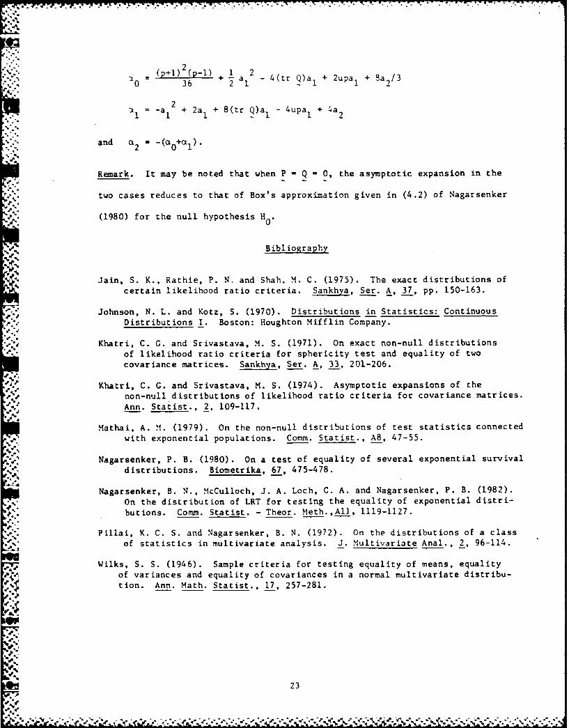
(+l)2()1 2 2..w. "(_P1 (l)(p-1) + a 2 (t Q~ + 2upa I + 8a2/3

20E, = -a12 + 2a + 8(:r Q)a 4upa2 + a2

and CL2 (O+l )2, 0

Remark. It may be noted that when P - Q 0 0, the asymptotic expansion in the

two cases reduces to that of Box's approximation given in (4.2) of Nagarsenker

(1980) for the null hypothesis H* 0*

%- Bibliography

Jain, S. K., Rathie, P. N. and Shah, M. C. (1975). The exact distributions ofcertain likelihood ratio criteria. Sankhya, Ser. A, 37, pp. 150-163.

Johnson, N. L. and Kotz, S. (1970). Distributions in Statistics: ContinuousDistributions I. Boston: Houghton Mifflin Company.

Khatri, C. G. and Srivastava, M. S. (1971). On exact non-null distributionsof likelihood ratio criteria for sphericity test and equality of two

covariance matrices. Sankhya, Ser. A, 33, 201-206.

Khatri, C. G. and Srivastava, M. S. (1974). Asymptotic expansions of the

non-null distributions of likelihood ratio criteria for covariance matrices.Ann. Statist., 2, 109-117.

Mathai, A. M. (1979). On the non-null distributions of test statistics connectedwith exponential populations. Comm. Statist., A8, 47-55.

Nagarsenker, P. B. (1980). On a test of equality of several exponential survivaldistributions. Biometrika, 67, 475-478.

Nagarsenker, B. N., McCulloch, J. A. Loch, C. A. and Nagarsenker, P. B. (1982).On the distribution of LRT for testing the equality of exponential distri-

$2: butions. Comm. Statist. - Theor. Meth.,All, 1119-1127.

Pillai, K. C. S. and Nagarsenker, B. N. (1972). On the distributions of a classof statistics in multivariate analysis. J. Multivariate Anal., 2, 96-114.

Wilks, S. S. (1946). Sample criteria for testing equality of means, equalityof variances and equality of covariances in a normal multivariate distribu-tion. Ann. Math. Statist., 17, 257-281.

23

Irrotational and Solenoidal Waves

in General Coordinates

by

D. A. LeeAir Force Institute of Technology

Abstract

Tensor analysis and some identities are applied to make tolerably convenient*L forms of equations for irrotational and solenoidal components of elastodynamic

displacement fields, valid in arbitrary admissible curvilinear coordinates.

Ilttroduc tion

Displacement fields of elastodynamic waves. i.e. suitably smooth vectorfunctions u(z,t) which are solutions of the Navier-Cauchy equations

a2V(V.U)-b 2 VxVXU= a

(2)

t 2

can always be written as sums of irrotational and solenoidal vector functions, inthe form

",=Vo(y,zt)+VxA (2)

P. where the vector function A(z.t) is solenoidal. i.e.

V.A-O (3)

(Reference [1]). The scalar jo satisfies the scalar wave equation

a.-0.= a-t"2(4)

and the vector A satisfies the vector wave equation

b2V2A= 2 A (5)

in (5).VA=-V(V A)-VxX

=-VAVxVxA

.. in view of (3) (Reference [2]).

P

.24

I$.1"t

4 ' , , , . . ... .. . . . . .. . .... . . . . . . . -i"t. . .. , . .. . : .. _ ,:!,",: " % " -,' ., , . -_ . " - -" " ' -> "" .. \ - .. ' '

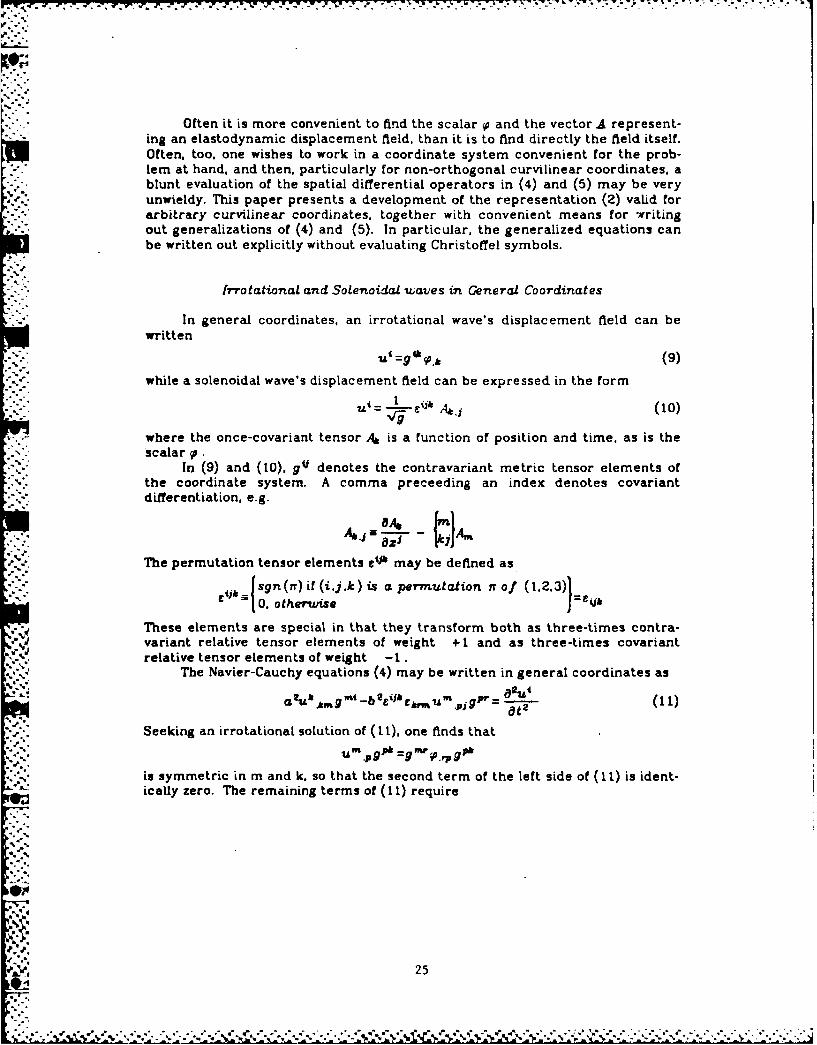
Often it is more convenient to find the scalar 0 and the vector A represent-ing an elastodynamic displacement field, than it is to find directly the field itself.Often, too, one wishes to work in a coordinate system convenient for the prob-lem at hand, and then, particularly for non-orthogonal curvilinear coordinates, ablunt evaluation of the spatial differential operators in (4) and (5) may be veryunwieldy. This paper presents a development of the representation (2) valid forarbitrary curvilinear coordinates, together with convenient means for writingout generalizations of (4) and (5). In particular, the generalized equations canbe written out explicitly without evaluating Christoffel symbols.

_rrotational and Solenoidal waves in General Coordinates

-:' In general coordinates, an irrotational wave's displacement field can be

written

- 9 90.t (9)

while a solenoidal wave's displacement field can be expressed in the form

u _- (10)

where the once-covariant tensor A* is a function of position and time, as is the'scalar 9.

In (9) and (10), gO denotes the contravariant metric tensor elements ofthe coordinate system. A comma preceeding an index denotes covariantdifferentiation, e.g.

• - . .. -A,.j a 8Zj A ,

A': The permutation tensor elements 06J may be defined as

sn (r)o. tif (i..k ) is a permutation rr of (1.2.3)}

These elements are special in that they transform both as three-times contra-, variant relative tensor elements of weight +1 and as three-times covariant

.-. relative tensor elements of weight -..,.: The Navier-Cauchy equations (4) may be written in general coordinates as

'a. 2Uh .. 9 ' -b t11h ,,u" Pjgp - of 211

Seeking an irrotationaL solution of (11), one finds that

, um.,gP =gf?.,gph

is symmetric in m and k. so that the second term of the left side of (11) is ident-ically zero. The remaining terms of (11) require

25

I °.................'- - - -

% la

- .-- --

..].' . . . . .. . . . . . . . . . . . . . . . . .

which will surely be met if

.g j. j (12)

One may take (12) as the defining equation for irrotational waves.Turning to solenoidal waves with displacement fields of the form (10). one

sees that

i .7. ;7"U "". Ml =i~ - . "/ At.jn =- 0

by the symmetry of At.jm with respect to j and m, so that now the first term onthe left side of (II) is identically zero. The remaining terms lead, after some

. ma,-ipulation, to

% %a2A L'k b2L..Em gpnA =0 (3

for which it is sufficient that the quantity in square brackets is identically zero.

But that condition leads, after use of the identity

~rto

But the defining tensor At of the solenoidal waves is itself solenoidal. so that

S. iA9,p z0 (14)

Then the defining equations for a solenoidal wave may be written as (14),together with

One could, of course, have written (12), (14) and (15) as tensorially con-sistent generalizations of (4).(3). and (5), respectively. It is well, however, tocarry through a complete treatment, starting with explicit definitions (9) and(10), to be certain the work is self-cons istent.

Moreover, while the forms of tensor equations (12) and (15) are succinctand easy to remember, these forms aren't usually the most convenient ones touse for writing out the detailed statements which those equations imply in agiven coordinate system. Direct evaluation of (15), for example, usually

. ~requires evaluation of ChristotTel symbols and derivatives of Christoffel symbols.Explicit "unfolding" of (12) for a specific coordinate system is made easier

a -.

.. "

26

,k AN.

by the well-known identity

ax. i (16)

by virtue of which (12) is equivalent to"| 9= f _ IO (17)

*/* Explicit writing-out of (15) is probably simplified in most cases by the fol-

lowing considerations: The elements T4, defined by

are once-contravariant (oriented) tensor coordinates. Also, they may beevaluated explicitly without evaluating Christoffel symbols, since

1 k8)

and the last term in (18) is identically zero by virtue of the symmetry of the

Christoffel symbol in its lower indices j and k, and the anti-symmetry of e4k in

those indices. Thus the St.

iai7- = g*- r, a

are once covariant, oriented tensor coordinates. Repeating the previous argu-

ments of this paragraph then shows that the R 1 ,

gi"n 8R .C

8 -- Ygm=- L, i -r -

are once covariant tensor coordinates, which can be written out without evaluat-

ing Christoffel symbols. In rectangular Cartesian coordinates.024.

Now. the quantity

V E . m " A..r,

appearing in (13) is also a set of once covariant tensor coordinates. In rectangu-

lar cartesian coordinates.

VI = m aA* 2 n R

27

" - % % *. - o° . . -. ° - .. - % o - . °° % % ° • ". . , °° = - ,% - % * •- •- . °- . ..-.. .

j . _ + +:, : , + +.+ .+ + +. + . +. : + . . . . . . . . . . . . .. . . .. . ..+ + . . .. . . . . . . .. - ' " -

But then R=Vk, . since coordinates of a given tensor character which are equalin one coordinate system are equal in all coordinate systems.

Thus a set of equations equivalent to (14), (15) is (14) and

Z fg 84 _2A. 19-mnp '* ,_ - (19)

, ,+.. Equation (19) is likely to be more convenient for writing out than equation (15).since no Christoffel symbols appear in (19). Moreover, the operations on the leftside of (19) can all be accomplished by fairly straightforward matrix multiplica-tions and differentiations.

References

1. Sternberg. E., Arch. Rat. Mech. Anal. 6 , 34 (1960)

2. Achenbach. J. D.. Wave Propagation in Elastic Solids Section 3.4, pages 85'S. ~ f. American Elsevier, New York. 1973

3. Sokolnikoff, 1. S. , Tensor Analysis. page 59. Wiley. New York, 1964

'2

'p

'S

"F.

! 4

SOME PROBLEMS OF ESTIATION WHEN SOME

PRIOR INFORMATION IS AVAILABLE

Albert H. M.oore

Air Force Institute of TechnologyWright-Patterson Air Force Base

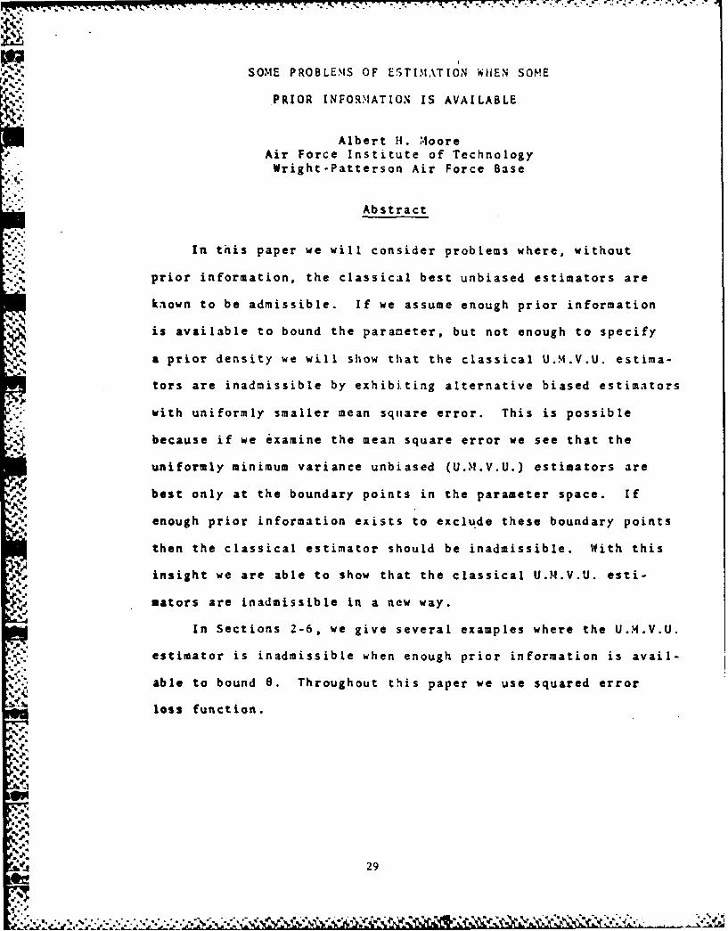
Abstract

In this paper we will consider problems where, without

prior information, the classical best unbiased estimators are

known to be admissible. If we assume enough prior information

is available to bound the paraneter, but not enough to specify

a prior density we will show that the classical U.M.V.U. estima-

tors are inadmissible by exhibiting alternative biased estimators

with uniformly smaller mean square error. This is possible

because if we examine the mean square error we see that the

uniformly minimum variance unbiased (U.M.V.U.) estimators are

best only at the boundary points in the parameter space. [f

enough prior information exists to exclude these boundary points

then the classical estimator should be inadmissible. With this

insight we are able to show that the classical U.?t.V.U. esti-

mators are inadmissible in a new way.

In Sections 2-6, we give several examples where the U..4.V.U.

estimator is inadmissible when enough prior information is avail-

able to bound e. Throughout this paper we use squared error

loss function.

29a,.,, .v. .,v..... .. : . r . :: : .. .

-.1 T 3 7 27p 7 -

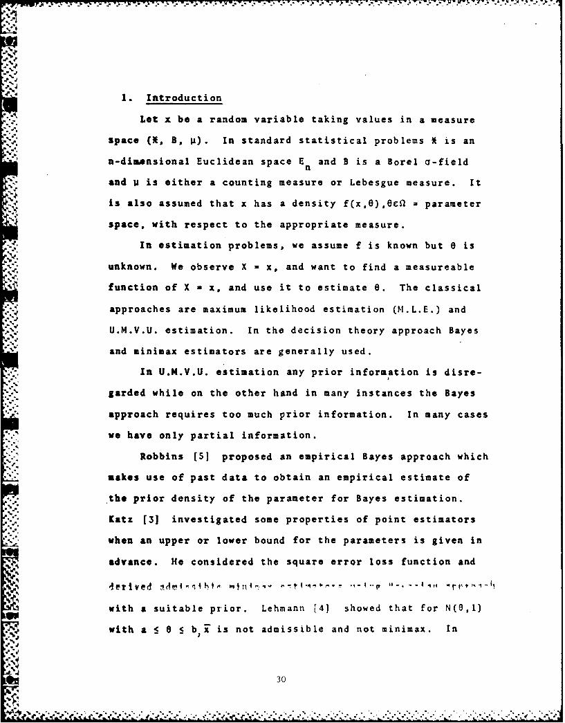
1. Introduction

Let x be a random variable taking values in a measure

space (M, B, P). In standard statistical problems X is an

n-dimensional Euclidean space E and B is a Borel a-field

and p is either a counting measure or Lebesgue measure. It

is also assumed that x has a density f(x,O),Oca =' parameter

space, with respect to the appropriate measure.

In estimation problems, we assume f is known but 0 is

unknown. We observe X = x, and want to find a measureable

function of X a x, and use it to estimate e. The classical

approaches are maximum likelihood estimation (M.L.E.) and

U.N.V.U. estimation. In the decision theory approach Bayes

and minimax estimators are generally used.

In U.N.V.U. estimation any prior information is disre-

garded while on the other hand in many instances the Bayes

approach requires too much prior information. In many cases

we have only partial information.

Robbins [5] proposed an empirical Bayes approach which

makes use of past data to obtain an empirical estimate of

*the prior density of the parameter for Bayes estimation."os

Katz [3] investigated some properties of point estimators

when an upper or lower bound for the parameters is given in

advance. He considered the square error loss function and

iertved II... d - I4 -,- 4 -1 - . "r - "- "- - 4 -oil rr t, -

with a suitable prior. Lehmann [41 showed that for N(O,1)

with a 5.8 S b ! is not admissible and not minimax. In

30

* .- ~ .... ~ - ..

addition he showed that if 0 > a, then x is minimax but not

admissible. Skibinsky and Cote [61 showed that with certain

prior information about the distribution of 0 for the

binomial x is inadmissible, and in a similar fashion he

showed that x is an inadmissible estimator for the mean of

the normal density. Kale [21 showed that for truncated

parameter spaces the M.L.E. is inadmissible by showing it

is not a proper Bayes estimator for the exponential family

S..; of densities with continuous parameter space. Blum and

Rosenblatt [1] discussed Bayes estimation where it was

assumed that the family of distributions which the prior

came from is known.,"

2. The Binomial Distribution. Let X be an observa-

tion from a binomial distribution with density b(x,n,e) *

eX(1-8) n 'x , 0 1 8 S 1. The statistic X is a completeXsufficient statistic for 0. The best unbiased estimator 01

of 0 is x/n. The risk of e1 is given by

R- (8) -- (1)01

Consider an estimator e of the form 0 * k" The2 2 V

!5 value of k which minimizes the mean square error is easily

seen to be

ka .2k -2 0

0(10 * &! 1I -o • 2-'-- + e --n TI

31

.. Pq

A7

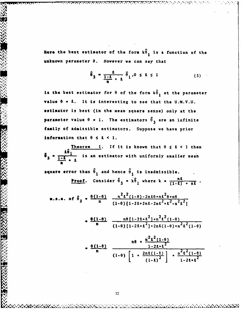
Here the best estimator of the form ke is a function of the

3 0 t L 1 (3)

is the best estimator for e of the form k61 at the parameter

value 6 - L. It is interesting to see that the U.M.V.U.

estimator is best (in the mean square sense) only at the

parameter value e a 1. The estimators 93 are an infinite

family of admissible estimators. Suppose we have prior

information that e S I < 1.

Theorem 1. If it is known that 9 1 t < 1 then

63 -.- is an estimator with uniformly smaller mean

square error than a8 and hence e is inadmissible.

Proof. Consider a = k8 where k a---- 3 1 (1-A) nA

2 2

" B.S.*. of 6$(ln oe)[l21+2nt.2nt2+L2_.n 2]

n (1-6) n 1-1 n2t2 O'e)

1 ((-)1-121-2+t

32

.- ..... .,-.-... ... . . . . . . . .. ... . . . . . .. , . . . . . • . ;

.. ,, , ,,. .. ,,,.,,.... .'.'...0.-,'-',), ., - 2.'L., ., . : . ',.'

n8n 2 t 2 11-2)/l-2t -2

n 2n+(1-O) (2 n22 2(lL)"1(l-0)/1-2L t;: (l-L)

Since e S t the fraction 2n,(1-) > n6. Therefore

R- (e) < eo-e) R^ (8)3 n1

and hence e is inadmissible.1

3. The Poisson Distribution. Consider the Poisson

density

•- x

f(x,x) eAA' x a 0, 1, 2, .(4)

Let x1, ..., xn be a random sample from a Poissonn

distribution. Let I a xi/n. A is a U.N.VU. estimator

of A with risk R- (A) a A/n. Consider the estimator A2 of

the form A2 - kA 1. The value of k which minimizes the mean

square error is easily seen to be

km A2k (S)A2 , /n

Therefore an estimator of the form

u A l > 0 (6)

is the best (in the mean square senst) estimator of A which

%! 33

.% .%

S%,

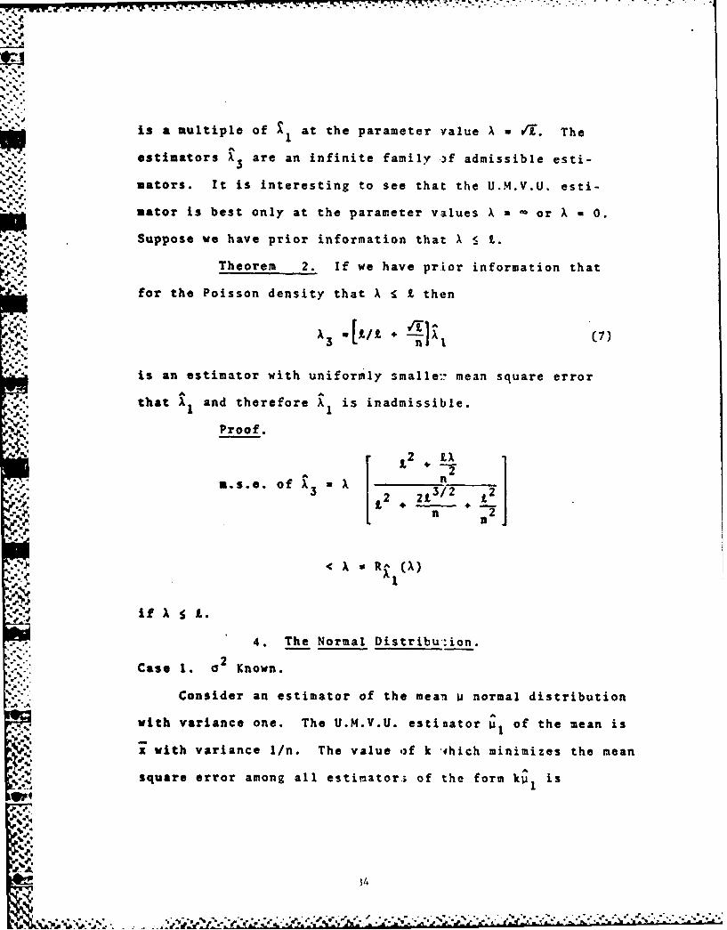
is a multiple of at the parameter value A /I'-. The

estimators X are an infinite family .f admissible esti-

mators. It is interesting to see that the U.M.V.U. esti-

.ator is best only at the parameter values X u - or A . 0.

-.P. Suppose we have prior information that X 5 L.

Theorem 2. If we have prLor information that

for the Poisson density that A I L then

A3 i x ~.A (7)n

is an estimator with uniformly smalle:7 mean square errorKIWIA

that A and therefore A is inadmissible.

Proof.

,,,.. £2 EXL/2

2,) 1K 2 2

if XS Z.

4. The Normal Distribu:ion.

02Case 1. aKnown.

Consider an estimator of the mean U normal distribution

with variance one. The U.M.V.U. estinator P, of the mean is

x with variance 1/n. The value ) k ihich minimizes the mean

square error among all estimator:; of the form k 1 is

..A

314

K. Q7(

l/n + U

Therefore an estimator of the form

2 1rn + L x where L _ 0 (9)

is the best estimator which is a multiple of p at the

parameter values i2 L. It is interesting to note that the

U.M.V.U. estimator is best only at the parameter value m.

Every one of the above estimators is admissible.

Suppose we have information that the mean is bounded,* that is p 2 < 1.

Theorem 3. If we have prior information that

U2 < I then 2 is an estimator with uniformly smaller mean

square error than u, and therefore 11 is inadmissible.

". .Proof.

1 J2/n + P 2 /n 2

M.s.e. of 2 = 2 /n l /n

I + 2/n + /n 2

a un L2 +

S~/n..(L + 21in + l2..

22

Case 2. a Unknown.

With the variance unknown, x = l is the U.M.V.U. esti-

mator of u with variance a2/n. The value of k which

.3

.4% 35

- . - * . . - - - - - - . - - . - , ,.-.-, _ , , . L - - : - - ' :" . . : ' ' " .' ' " .+' ' -• ' '- - - .' ' :, - " - :

minimizes the mean square error among all estimators of the

form kul is

k2 I where S2 (2k 2/n +2 _1 2

ns

Consider an estimator of U

.2 W i(n) + I)

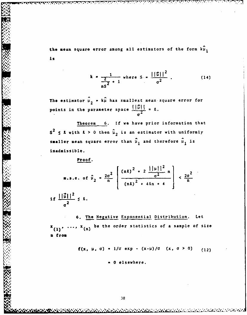
The estimator U is best among estimators of the form k2 2

along the lines La2 , 2 in the parameter space.

Theorem 4. Suppose we have prioir information

that < then U" is an estimator with uniformly smaller2

aAmean square error than U I and hence is inadmissible.

Proof.L

-*. -, I- L2 a 22 + 1 21/n a 2 0--

,.se. of ii~ + * /n a, _ . . .+ _-

n2i. . n/n n 2Jn

22

..... I. The Bivariate Normal Distribution.

Case 1. Covariance Matrix I.

.% Consider a bivariate normal with variance-covariance

matrix I and mean vector unknown. The U..V.U. estimator

36

of A = ( Iy) is l * (P y)" It has been shown to be

admissible. The value of k which minimizes the mean square

among all estimators of the form kp1 is

4-2

kI L. (12)(2/nZ) •I

The estimator

i - A _ _

Ln2 = _(21n) + . Il (13)

is best in the mean square sense among estimators of the form

k1It for points on the sphere Ux2 y y I in the parameter

space, Again the U.M.V.U. estimator appears best only at

the points in the neighborhood of the point at infinity.

Theorem S. If I lIl I St, L > othen 2 is an

estimator with uniformly smaller mean square error than p,

and hence P1I is inadmissible.

Proof. 1 124...L2 + 2

u.s.O. of <2 2 *R2 n " 2 2 4-- 4 n

2 2Case 2. Covariance matrix I a a Unknown.

The U.M.V.U. estimator for the mean is again

V1.(Y,Y) with variance 2o2/n. The value of k which minimizes

-p 37

the mean square error among all estimators of the form kv 1

k-' 2 where S. I I(I12-2 (14)

nS

The estimator V 2 x kU has smallest mean square error for

points in the parameter space 11241 =

a2

Theorem 6. If we have prior information that

S2 L L with L > 0 then j2 is an estimator with uniformly

smaller mean square error than Al and therefore A is

inadmissible.

Proof.

2222 2M. . .of P<

of-a.A.T (n1) 2 + 4Xn 4

. .

if < ,.o2

6. The Negative Exponential Distribution. Let

1x(J ' *.n. be the order statistics of a sample of size

n from

f(x, a, a) = 1/a exp - (x-j.)/F (x, a 0) (12)

= 0 elsewhere.

38

* i * l- [ V [ i - ' i .* . i " " * ~ . . .

Lot Z alx and Y l/n ( - ) The distri-i=2 (1)

bution of Z - np is rl,o) and the distribution of Y is

(n-l. o). The admissible U.M.V.U. estimator Pi for P is

Z/n - Y/n(n-1). The estimator P12 which has the smallest mean

square error among estimators of the form k I is the one with

IJ~2 1

k 1 =1wherea2 ,2 1 1

,. 2 (n) (n-i)

'.

S2 u252 *- Y (13)

Consider an estimator

13 + 1J, where 0 < . (14)

The estimator is best in the mean square sense among esti-

mators which are a multiple of a1 along the lines to2 2

in the parameter space.

Theorem 7. Suppose we have prior information2

that -< L then P is an estimator with uniformly smaller

mean square error than and hence is inadmissible.

Proof.

A ~ , 2 2 2 22m.S.e. of P u+ 2/n(n-l)I r2(n-) . ) 2L2* n(n-l)2 /a

r1 (n-) it + 2n(n-l)t + 1

<uR^ if P 2 / 2 .t.

39

S- -.-

REFERENCES

[1) B1um, J. R. and J. Rosenblatt. "On Partial a prioriInformation in Statistical Infe::ence", Annals ofMathematical Statistics, 38, 1967, pp. 1671-1678.

[21 Kale, B. K., "Inadmissibility oF the Maximum Likelihood

Estimator in the Presence of Prior Information",Canadian Mathematical Bulletin, 13, 1970, pp. 391-393.

131 Katz, Morris W. "Admissible and Minimax Estimates ofParameters in Truncated Spaces", Annals of MathematicalL Statistics, 32, 1961, pp. 136-142.

[4] Lehmann, E. L. Notes on the Theory of Estimation,- mimeographed notes recorded by Colin Blyth, University

of California, Berkeley, 1950,

(S] Robbins, H. "An Empirical Bayes Approach to Statistics",Proceedings of the Fourth Berkel.ey Symposium, Vol. I,Berkeley and Los Angeles, University of California Press,1956, pp. 157-163.

(6] Skibinsky, Mark Cote L. "On the Inadmissibility of Some

Standard Estimates in the Presence of Prior Information",Annals of Mathematical Statistics, 33, 1962, 539,548.

V..:

440

NAI9-.. " """' "'" """ . ",p" " "" ": """"""" " "" " " ' "" 1"

- -. . . . . . . . .

-a.--

NON-NULL DISTRIBUTIONS OF THE LIKELIHOOD RATIOCRITERION FOR THE SPFVCTRAL MATRIX OF A

GAUSSIAN MULTIVARIATE TIME SERIES

B. N. N"agarsenker

U. S. Air Force Institute of Technology

ABSTRACT

Let E(w) be the spectral matrix of a p-dimensional zero-mean stationary

Gausstan time series X'(t) - (X1 (t), X (2), ..., X (t)). In this paper, we

consider the test for the null hypothesis Ho: E(w) - (w). where ko(w) is a

known matrix for all wi against the alternative Hi E(w) c' Eo(w) and obtain

* the nu.1 and non-null distributions of the likelihood ratio criterion as

mixtures of incomplete beta or gamma functions. These representations are

well-suited for programing on a computer to find the exact power of the

test.

1. INTRODUCTION

Let X'(t) - (Z (t). .... I (t))be a p-dimensional stationary Gaussian

multivariate time series with zero mean vector. Let E(w) denote the

spectral matrix of X(t) so that

4(- o ((47 ()), (.k - i.2.....p)jk

jmmwhere a jk(W) r. itjk (8)0- denotes the cross spectral density2w $-~

function between X (t) and Y() and

tjk(s) - E(Xj(e).Xk(tts) ]

denotes the correspondtng cross covariance function. We assume that for each

pW the hermitian matrix E(w) is positive definite. Let

J~k-l.... .I", T t TIo

where e - - , * O, . .... T

dL. 41

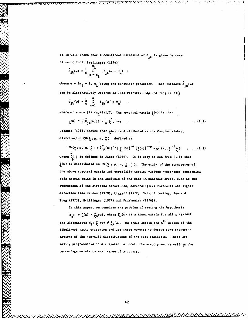
It is well known that a consistent estimatoi' of ak is given by (see

Parzen (1966). BrLllinger (1974)

.- -r I (W + )* M-n 1 jkEUer nzt -.Zat +:1.: n being the bandwidth parameter. This estimate M

a(19

ojk~ch) ([.1

where w' - w- (2 (n1L+I)]/T. The spectral matrix S(O) is hen

' s - (( )) - say

Goodman (1963) showed that A(w) is distributed as the Complex Wishart

Sdistribution CW( ; p. n. defined by

.. ) ;(7;p(n))_L Z (')- n IA(w)jn-p exp (-tr -LA) .el %, p, %

whare (.) t defined in James (1964). It is easy to see from (1.1) that

S(aa) to distributed as CW(S , p. a. E ). The study of the structures of

P 'd the above spectral matrix and especially testing various hypotheses concerning

this matrix arise in the analysis of the data in ougerous areas, such as the

vibrationis of the airframe structures, meteorological forecasts and signal

detection (see Haana (1970). Liggecc (1972, 1973). Priestley, Rao and

Tong (1973), Brillinger (1974) and KrishnaLah (1976)).

0eIn this paper, we consider the problem of testing the hypothesis

1 S , ~ ,(w) *,E (). where ko(w) is a known matrix for all w against

the alternative H M ( 7 (w). We shall obtain the hth moment of the

likelihood ratio criterion and use these moments to derive some represen-

tations of the non-null distributions of the test statistic. These are

easily programmable on a computer to obtain the exact power as well as the

percentage point. to any degree of accuracy.

42

.~~~~~~ 17 7. 777 7. 7 2 ~ * *-*.- -Z 7

2. SOa£ PRELIMINARI S

The following results and definitions are needed ir the subsequent

sections. The Mellin integral fransform of a function f(x) of a real

variable x, defined only for x > 0 is

M{(f(x)l,} - E(xs ') - xs-f(x)dx .0

where 9 is any complex variate. Under suitable restrictions (Titchmarsh (1948))

satisfied by all density functions considered in this paper, there is an inverse

formula or inverse Mellin transform

(1) - (21t)- f x-(Mf(x)lslds .(2.Z)_

....

c-i-

velid almost everywhere. A path of integration is any line parallel to the

imaginary axis and lying within the strip of analycity of M(f(x)Is).

Lamea 1. Lot

x(t) - p(x)dz

be the moment function of a random variable x with the distribution law

p(s). te

4 (t) - o( "k) .. .(2.3)

wItb reel part of t tending to * then $(t)' can be expanded as a factorial

series of the form

0(t) - 1-o An r(t+e)/r(t4.kn,). ... (2.4)

a being any arbitrary non-negative constant (see Nair (1940)

Lem 2. Let the asymptotic series Z Q xj

converge to the function g(x)J-I i

in the neighborhood of a - 0 (or be its asymptotic expansion when a - 0).

We then have

, *a(l ) +-I Bxi .(2.5)* i-Ii

where the coefficients Oj satisfy the recurrence relation

*i m k 0 J-k" so I ... (2.6)

(see Kalinin and Shalevskti (L971).

43

I. 1

..

Consider now the test for the null hypothemis H E(W) -E,(W)* where0 % %.

EO at a known matrix against the alternative N: E(W) w0 E 0 Proceeding

1o.-%

as in Anderson (1958. p. 264). it can be shown that the likelihood ratio

criterion is

(*/)p n - ) .. .

where. for convenience, we have suppressed w and written A for A(w). etc.

Alternatively A may be expressed as

A..e AIn etr (-A). ... (2.S)

w ,here A .CW (A. p. n. E' - o-... ,0

Lemma 3. Let z : pxp be a complex symmetric matrix whose real part is

positive definite and S: pxp be a hermitian matrix. Then

sf eexp(-tr z s) s a-p ds

"-. - rp (n) II

1.-in ... (2.9)

(see 0. 94 of JUm (1964)).

Lm 4. The h moment of the statisctc A defined in (2.8) is given by

3(A) Thez(-" ( .- " ," pe(2.10)"'" Zl~h) =('/n I t~h + h U+h' %.(.O

"Ot: Z(A ' ) - f CW(A. p. n. El 1. . d AA " A 0A

(/n)Pnh Irl-a I "h-p

% A A 0 JA t((El l

Using Leina 3. the result fc-'I owsa44

..

_ 44

%...

4 .'

4.:

Lemma 5. The following identity ts true:

"+ h r -(h+n)

( + h-p(h+n) -(hn) E -1

e, Pj + -p(h+n) t -(hn) (h4")(h () )E:-O EK KK(211h k...(.ll)

(I + ) k1

where M - I - and C (. ) is the zonal polynomial as defined in James (1964).

ethis is valid since h can be chosen so thatlIl - ch max nfI(1

1/- Lemma 6. The following expansion for the gamma function holds:

lo8 r ( h) - log (zw)h + (x+h-1l2)lo$ x - x

E (-1)' 3 (h) R (z).-"r(r+ll z +

where t x) ti the remainder such that I(x) . being a constantI'al

ladependent of x and a (h) is the Bernoulli polynomial of degree r and order

•q one.

3. NON-NULL DISTRIBUTION OF A, AS A MIXTURE OFINCOMPLETE BETA FUNCTIONS

In this section, we shall derive the non-null distribution of L - Xn

where A is given in (2.8). Using (2.10), the ht h oument of L under the

alternative hypokhsls Ls

9(L h E(z~th . n(h)

. (/n)Ph 11 (h) + hh Ii r..-(h,) . )

e-(a)

whore r . Using the inverse .ellin transform (see (2.2)), the density

a. f-inction of L is stiven by

'45

:4+.

* .-C a'• , ... ' , " € " .'_: . , ,' , :: ,' . . .:, , . ' ../ " '," . .: . - .' . , - -" , . ",", ' .:", - . ."", - ."" \ " -

,... ... . . . .

4

f (L) (rp (n)) (21ri)

-..--

c+t -h-I ph '%I (n+h) hI h hC ,rn r +dh.. (.2

Jc+- p

" We now use the identity (2.11) of Lenma S and write t - r+h to obtain

f(L) - K(p.n. r. L)

E-'" .o x V C(M) p(L) ...(3.3)

where

p(L) " (21)-1 Ic+ i. "L-t 0(t) dt ...(3.4)

C-i-

4() (lt) Pt Ck nP (t + k k+-. 5

and

K(p. a. L.) - I- l-" 1 (/n)-p" Ln-l

., Dy Lem 6. log O(t) may be expanded as

.;' 4.' P/2 + o -v + Elog #(t) log (21!) / log t L o(q ite.)

where the constants qr are given by

qV a (-)r'I ( EP 5 r1 (k(1 -a) / r(r+t)) ..(3.6)

and V a p /T Thus we have

.(e) * " v(2 )P/2 (1 + E,( /J)}

wheire the coefficients tr can be recursively computed using the relations

(2.6) and (3.6). In other words, the coefficients Ersatisfy the recurrence

relat~on

t E., k q I o " .. 8.(.S)r r k-IL k r-k,

, .

7 146

.4.

Now from (3.7) and (3.4) we get

p(L) - (211 (2w)912

fc + i L - t -v(L+ . Itr) dt ...(3.9)c-i- + r

The integral on the right hand side of (3.9) can be easily computed if v is

an integer and its value, by Cauchy's theorem of residues is 2xi times the

sum of the residues of L-t t'v (1 + fr/tr) at t - 0. This is easily seen to be

(21) (2w) p 1

2 E o0 k-log L)' -t/r(v+r)),

and thus from (3.9)

p(L) - (2n)p /2

E .O((-log L)v4' -I r I(v+r)) ...(3.10)

Then from (3.3). the probability that L is less than any value I 0 is" L k L L0

.(P n. El) E:k*O K1 2 CK p(L) dL, ... (3.11)

where

i r (e.~~~n 0. ) . ,P (r(n.1-u)) "1 I~t-n ,)-.K, (p. .,E1

S.,1

For computational purposes we let tpn-I andL

I vft-I.U (o0 ) - f0 LU -lot L) /r(v+) dL. ... (.)

lntelgrttng (.12) by parts, it can be easil.y shown that the following

recurrence relation holds:

%, ) - Ul

I (Lo) - (LU i (-log Lo)V+r-lI r(v+r) I Y.2,u(Lol/(U~l) *,.(3.13)

With this notation, (3.11) becomesk

PAL L K ., l " !-Ck q

Er-O Ir I v+r-1, u(Mo0 ... (3.14)

It is to be noted that (3.14) holds only if v /2 ii an integer and this

representation is computationally efficient in this case. However, if v is

not an integer. ve can appeal to Lemm 2 since in this case $(t) satisfies

(21)-p12 2(t) - O(t- v ) ... (3.15)

-4

47

-o ,*% S%

• .k. -

, ". . ..

Wd7

Then from Lemma i. we can expand (2'R)-p /2

0(t) in the factorial series as

(2w)-P 1 2

4(t) - 'v(I + E-0 (tr /t))

- 0 r(ta)/r(t+v+a+t) , ..(3.16)

where a is any arbitrary positive constant and can be chosen to govern the

rate of convergence of the resulting series. The coefficients R can be

explicitly determined as is done below.

Applying Lema 6 to each of the gamma functions in (3.16) we get

log (r(t4.a)/r(t+a4v+i)) --(v~i) log t + E7.1 (A /ts)ij

where

A iA - (-l) J-11B+ 1 (a) - B J+(v+a+i)l /J(J+l) ... (3.17)

Thus we have r(=.,)/r~t ,.. l) -(v41) . ci tlr(t+a) r(t+ i) - (1 + E (C ))...(3.18)

where by Lemm 2 and (3.17). Ct, can be recursively computed. Using (3.18) on

the right hand side of (3.16) we get

. I Equating the coefficients of like powers of t on both sides of (3.19). it is

easy to check the following explicit relations to determine RI:

rI iCi_ - t1 (L-1,2,3...) ...(3.20)

where 1 and CO 1.

Now using (3.16) in (3.9) and noting that term by term integration is

04 valid since a factorial series is uniformly convergent in a half-plane

(see Doetch (1971)). we have

p(L) - (2w)p/2 E ft ( 2

i -f Ci Lt {r(t+s)/r(t a..-.j)} dt , . .. (3.21)

We now use the well-known Integral (Titchmarch. 1948)

48

4%?'

(2"i)R t ci- x" (r(s+a)/r(s+a+v+j)) ds x a (l-x) v+Jl,

c-i-r(v+j)

and obtain

p(L) - (2w) p/2 --0 R L(la-L)+J-1/r(v+j).

Then from (3.3), we have the following exact noncentral c.d.f of L as a

%. A mixture of incomplete beta functions:k

P(L' <. O) - K.(p, n. EZ) Ek-O £ C (M)

..

"r""- 1-0 D t 1 L 0 (n ~a , v+i)/r(v+t) , ... (3.22)

5:! whereD, = (n+a, v+i) RI

'p. and

3 1 (p.q) " (I(p'q)}l fx X p-1 (-x)q'-l dx0

is the Incomplete beta function.

As a particular case, putting Z0 - I.e.. K" 0 * we get from (3.22) the

null diatribution of L as the following mixture of incomplete bets functions:

--. < Lo) - h ( p" n. I ) E-0 =1 a (na. .i, ... (3.23)

-. *.-"where 0; is the coefficient D with ki - 0.

4. NON-NULL DISTRIBUTON OF A AS A IXTUIE OFINCO#ULETE GA?*(A FUNCTIONS

Let Ll - -2q log A, where A is as in eq (2.8) and q is am adjustable

constant which can be chosen to govern the rate of convergence of the resulting

series and 0 < q < a. If C(t) is the characteristic function of L1 then

fro (2.10) we have

c(t) - (n/e) tIt r' (n(l-Zqit)) [?(n))p p

i -nqit -n(l-2qit)%-, I 1 I 'u ' 11 ,. .(,.1)

449

mqk!

k--.,

where,,°4 asdfndi oatn 16)

_o 1(,) npi k-lg ' nki' n 2p 1it/e

o(t) p n(-qtt). K 0 (1-2r')

- ...(4.3)

vhere

..,"- rp (&,K) - "K ? p(a)

, , as defined In Constantine (1966).

%'" Using Lemm& 6. we obtain after some simplification

log H(t) P logl 2r * k iog n pn loqtn/e)

- log (n()-2qit)) + (l-2qic) r .... (4.4)

jl r-l r 7

w here v p p2/2 and

so thatR(t) - (2w)p

12 nk (,,,)

P" (n(l-Zqit)}

-v (1 - E* . A (1-Zqt)-r) ... (4.6)

where the coefficienta Ar can be recursively computed using (4.5) and Lemmr 2.

Noting that (1 - Oit)" is the characteristic function of the game density.

* (.,x) - r(-XS i > 0, d 0 0 . 80

S.. we have from (4.2) and (4.6) the density of L- -2qlog)

f(L~~ ~ ~ K (.H)E)

k1

A (2q. L), A0 I ... (4.7)CrO r 1 r'v 1) A0

where

K2(p, n. - (2,)P12 (rile) pn / i in nP,- (r(n4.+l-))- I ... (4.8)

and the noncentral c.d.f of L is then the following mixture of incomplete

gamme functions

50

P(L) x) t-K2 (p, n. Z) r.O K M kC (M)ki

V.0 r r-v

where

c (e.x) a (s~r( ))- ! g (0,y) dy

Remark.

(1) Taking Z0 . or -0 in (4.9), the c.d.f of L , -Zq logA in

the central case is the following mixture of incomplete gaam functions

F(L ! x) - K2 (p. a, 1) Z A; -v G, (Zq. x). ...(4.10)

where A' is the coefficient A with k *0

r r r" (2) Taking q-l. we obtain the representation of the c.d.f of LI in the

central case as a mixture of chi-square distributions..1'

The representation* of the c.d.f's of the likelihood ratio criterion

A obtained n this paper enable one to compute the exact power of the tests

using only the tables of zonal polynoials and tables of either the incomplete

beta or am functions and are in s form which can be easily prograesed.

Further, the introduction of the adjustable constants to Sovern the rate

of conergemce and the recurrence relations (3.8), (3.13) and (3.20) are*

well-suited to computations of power as well as percentage points for test*

,I of significance.

3. REZINCES

1. ANDERSON, T.V. (1958) Introduction to Rultiveriate Statistical AnalysisVley. Niew York.

2. BRILLINCER, D.R. (1974) Time Series: Data Analysis and Theory. Holt,Rinehart and Winston, New York.

3. CONSTANTINE. A.C. (1963). Some non-central distribution problems Inoultivarlate analysis. Ann. Kath. Statist. 34, 1270-1284.

4. DOETSCN, G. (1971) Guide to Applications of ths Laplace and Z-transformations..3Van Noitrand - Reinhold, Ncw York.

3. .

-° 3

3...

- '..-

r S. GOODMM, N.R. (1963). St.atistical Analysts bascd on a certain multi-variate complex Caussian distribution, (An Introduction). Ann.

% ,Math. Statist., 34. 152-177.

6. HANNAM, E.J. (1970). Multiple Tim* Series, Wiley, New York.

7. JAMES, A.T. (1964) Distribution of matrix variates and latent rootsderived from normal samples. Ann. Math. STat.. 34, 4175-501.

S. KALINI, V.M. and SHALAEVSKII. O.V. (L971) tnvestigations in ClassicalProblems of Probability Theory and Mathematical Statistics:Part I.. Consultants Bureau, New York.

9. KRISHIAHAJ, P.R. (1976) Some recent davleopments on complex multivariatedistributions. 1. Multivariate Analysts, 6. 1-30.

10. LIGGET, JR, W.S. (1972) Passive sonar: fitting models to multipletime series in Proceedings of the NATO Advanced Study TIstituteon Signal Processing. Academic Press, New York.

-, 11. LICGETT, JR., W.S. (1973) Determination of Smoothing for Spectral .4atrixEstimation. Technical Report,. Raytheon Company, Portsmouth,Rhode Island.

12. NAIl U.S. (1940) Application of FaCtorial Series in the Study ofDistribution Laws in Statistics. Sankhya, 5, p. 175.

13. XIESTLET. H.S., SUBBARAO, T. and TONG, H. (1973) Identification of thestructure of multivariabe Stochastic Systems. In MultivariatAnalysts III (P. R. Krishnaiah, Ed.) Academic Press, New York.

14. TZTCIRS, E.C. (1948) Introduction to the Theory of rourier Integrals.

Oxford University Press, London.

N'.

*52

Probability of Destruction of a Point Target in Space

1. S. Przemieniecki

Air Force Institute of TechnologyjVrfight-Pdtterson Air Force Base, Ohio

Abstract

This paper presents an analytical method for the calculation of the proba-Zp bility of destruction of a point target in three-dimensional space for a given

aiming offset and a spherically symmetric Gaussian distribution of the pro-bability density function. The resulting probability is presented in terms oftwo non-dimensional parameters expressed in terms of the aiming offset rO.the lethal radius &. and the variance A,~ The resulting spherical error prob-able is compared with the corresponding two- and three-dimensional cases.i.e. the circular and linear error probables. The limiting case of zero aim-ing offset is also discussed.

Introduction

When the dimensions of a target are small compared with the effectiveradius of the weapon within which the target can be destroyed. the targetitself can be represented by a point in the mathematical model of theattack. For example, such a model may represent the case of an anti-ballistic missile (ABM) with a nuclear warhead used to destroy an incomingreentry vehicle. Here the size of the target itself is minute in relation tothe lethal radius of the ABMI warhead and consequently the target can betreated as a point target. Due to systematic errors which occur in anyweapon system the actual aiming point (mean point of detonation) will notcoincide with the target and the usual randomness characteristics of the

* .. weapon will produce the typical scatter around the mean point of detona-tion. The systematic error can be accounted for by specifying the aimingoffset distance from the target while the randomness error can bedescribed by the usual standard deviation in the three-dimensional proba-bility density function.This paper presents the analytical method for the calculation of the proba-

bility of destruction of such a point target in space for a given aiming offsetand specified lethal radius. The probability density function (PDF) describ-

% ing the weapon scatter in space is assumed here to be given by a three-dimensional Gaussian distribution with equal variances. The probability oftarget destruction is shown to depend on two non-dimensional parametersexpressed in terms of the aiming offset ro . the weapon lethal radius R. andthe standard deviation a . Furthermore, the paper defines the sphericalerror probable (SEP) as a relationship between the lethal radius parameterR/ a and the aiming offset parameter ro/ cr and then compares it with thecircular error probable (CEP) and the linear error probable (LEP) . Theanalysis includes also a discussion of the limiting case of zero aiming offset.

q 45

: Abstr53

Evaluation of the Probability

The analysis of the probability of destruction of a point target for two-dimensional cases has been treated extensively in the past by variousauthors and tabulated results are available - . This paper provides anatural extension of this analysis to three-dimensional cases which may beof importance in determining the effectiveness of an ABM system. It will beassumed that the aiming offset point (i.e. the mean point of detonation) isat a distance ro from the target placed at the origin of coordinate axes as

-- shown in Figure 1.

z

Mean point ofdetonation /

r V

Targe d9

" .",Fgur 1agt , . Tardet in space

.'.'. -" [

" -"the z-axis so that the three-dimensional probability density function based

-~ ~ n equal variances a can be expressed as

_y2

-.... P(=.Y.-)= e--p

Figureo) 1.o Tage isa ce

_' ._r2_ _ rr 0 cos (

where the relations r 2 =z 2 +y24-z2 and z =rcosp were used.The probability of destruction of the target is calculated from the integral

P=fffp(X.Y.Z )rsinjdrdjt~d.€.; ~~~ * 2n r f se,. I_} fcos v

ex" 1 2p - o r sinpdrdjpdO;.," ." V Oa-J 0 0 a 2a2j t

.. L:...-r)2

-( =r) ex .- rexcp r-rI ro 2

54

.a - t 6.g -

Subsequent integration is possible with the substitution of the followingvariables:

. .. ,.p--r/ [,ral (3)

e, ¢* ( The symbol p denotes the quantity RI [v/7] when used as an integrallimit or as a parameter.)

-:::,: oo~ro / 4, (4)

.. 'p -P (5)

-Y V" =p +Po (6)

Substitution of the above variables into Eq.(2) leads to

P= f (upo)exp(-,u)du- f t v-.f" " " ' PC

which can now be integrated. This results in an expression in terms ofexponential and error functions, given by

P =P(R/ u.ro/ u) (8)

= 9-epfpp)J exp[-(p-po)2

+VITPa[II (P+p0)+erf (P-Po)J)

Equation (8) is plotted in Figure 2 for a series of values of the offset param-eter r0/ a . When to/ r=O (i.e. when p0=O) then Equation (8) reduces to aspecial case of zero offset. Since P0 appears in the denominator of Equation(8). L'Hopital's rule can be applied to obtain the limiting value when ?o=0.This leads to

P(R 0.)=-2PIR/,0) e- p (-p,) + erf' (p) (9)

* .5%q55

~~.8

.6

.. 4

0 1~- l2 3 4 6 6

R/a-o ___ - -.

IRI

Figure 2

Probability of destruction of a point target inspace for a given aiming offset ro a and thelethal radius RI a

Spherical Error Probable

For the case of zero aiming offset r0=0 the Spherical Error Probable (SEP)* is defined as the radius R for which 5O7.of all detonation points in space will fall

within the radius and the remaining 5O7.will fall outside this radius. Thus if R-~ represents also the lethal radius any detonations within the radius R wilt destroy

the target. This concept can also be extended to non-zero values of ro This is

obtained simply by equating P in Equation (5) to 1/2. so that

+%"rpor(p+poerf (p-po]]1 (

Equation (10) gives a relationship between RI a and T 0 / a for the Spherical Error

.¢..4

Proabl. Tis elaioshi isplotediFigure 3,wihsosclal2o h

lethal hal radius R / nrasdwtanicesinheoftprmtr a

t o r achiee 0.5(ie. 50,7 )zeroii oft = tare dercion. Fror Probable R(SEP)

56

.5'dfnda h aisR o hc 0o ~ eoaio onsi pc ilfl

withn te raiusandthe emaning50 illfalloutide hisradus. husif

-...... *.71

i.e. the lethal radius is approximately equal to the aiming offset.

4 ~~'

3

R

(r 2

.55P

0 12 3 4

'p.,/1T

Figure 3

Variation of linear, circular, and sphericalerror probable with the aiming offset rg/ a andthe lethal radius RI a .

For completeness. it is interesting to compare similar relationships for the

circular and linear errors probable. Thus using results from Reference [1) it can

be shown that

g~h..=1/ 2(11)

represents the required relationship for the Circular Error Probable (CEP),

where

g 1 1'-erp(-p) (12)

= =2 2(n - ) 2)+Fg* g, - l -x( _) (13)

557

h, 0("-exp(p')(14)

with p and Po deflned by Equations (3) and (4). except that R and r 0 refer now tothe radii in the two-dimensional impact plane containing the target.

It can be demonstrated that the corresponding relationship for the LinearError Probable (LEP) for a point target in one-dimensional space (range) is givenby

Lf [R-r ((R+r 0 ) 11/ (15)

where R refers to the lethal range and r 0 is the linear aiming offset. Both rela-tionships for the circular and linear cases are also plotted in Figure 3.

AcknowledgementThe author wishes to thank Dr. David A. Lee for his assistance in program-

ming different computer solutions presented in this paper.

References

1. Brennan. L. E. and Reed. I. S.. A Recursive Method of Computing the Q-Function, IEEE Transactions on Information Theory. Vol. 11. pp. 312-313, 1965

2. Burington. R. S. and May, D. C., Handbook of Probability and Statistics withTables. Sandusky, Ohio. Handbook Publishers, 1953

". 3. Groves. A. D. and Smith, E. S., Salvo Hit Probabilities for Offset Circular Tar-gets. Operations Research. Vol. 5. pp. 222-228. 1957

4. Marcum, J. I.. Table of Q-Functions. Rand Report RM-339. The Rand Corpora-

tion, Santa Monica, California, 1950

5. Rice, S. 0. ., Mathematical Analysis of Random Noise. Bell System Technical

Journal, Vol. 24, pp. 46-156, 1945

S. Solomon, H., Distribution of the Means of a Random Two- Dimensional Set,Ann. Math. Stat.. Vol 24. pp. 650-656. 1953

'°

5

/ 58

V7:.], ., e ' ,,',.- -. , .*,.1.....',"."."v .. ''''"•,

*k .1.-7777r.W

A NEW VARIATIONAL PRINCIPLE FOR ELASTODYNAMIC

PROBLEMS WITH MIXED BOUNDARY CONDITIONS

by

Peter J. Torvik

Professor and Head

Department of Aeronautics and Astronautics

Air Force Institute of Technology

Wright-Patterson Air Force Base, Ohio 45433

4Abstract

A new variational principle is presented which enables the use of a direct

approach to obtaining solutions to problems in elastodynamics with mixed boundary

V conditions. The principle may be viewed as a modification of Hamilton's prin-

ciple, in which the requirement that virtual displacements do not satisfy the

displacement boundary principle to general elastodynamics. A procedure is given

for using the method to determine the natural modes and frequencies of membrances

and plates having mixed boundary conditions.

59

*~~~~~~~~~ % * = ~ * . * ... . . ' .x

1. % .o-q

.

,%

I. The Variational Principle

%, In the application of Hamilton's principle, it is necessary to seek an

extremal value of the Lagrangian function over a class of admissible virtual

displacements which vanish, for all time, over the portion of the boundary

Iwhere the displacements are to be prescribed . For many problems, finding such

functions is not readily done; therefore it is of interest to investigate the

possibility of extending the class of admissible functions to include functions

which do not satisfy tfhe boundary conditions on those segments of the boundary

where tractions are prescribed, nor on those portions where displacements are

prescribed.

e. This relaxation of requirements on the trial functions is precisely that

% .. 2permitted in the use of Reissner's principle , which is applicable to both the

static response the the simple harmonic motion3'4 of elastic systems. It is

of interest to begin as with Hamilton's principle and to derive a somewhat

%more general result.

We begin by writing a Lagrangian function

: .~ *L U U-K + A()

where the strain energy, U, of an elastic material is written as a func-

tion of strains,

U W(ei )dV (2)

V

the potential energy of conservative external forces is written as

Aei- Ti ud - I Fiu dV (3)

S V

60

.1' ~~ - ~' - s

and the kinetic energy is expressed as

K = I Pu adV (4)

V

The volume of interest, V, is enclosed by the surface S = S + , where

Su is the portion of the boundary on which displacements are to be pro-

scribed, and S is the portion on which tractions, Ti , are given. The

body force, Fi, is presumed to be prescribed. The customary requirement

that the displacements satisfy a boundary condition

u U on S (4)

Jd *

is replaced by a constraint,

Cl "C J r1 (uI - uI )ds (5)

S

where the r are Lagrange multipliers. We assume, as in the further

generalization of Reissner's principle due to Washizu 9 that the atrains

and displacements may be varied independently. Thus, the requirement of.= I

satisfaction of the strain displacement equations is replaced by a con-

straint

C C2 = lj[ij - '1 (uij uj,i

V

where the cona denotes partial differentiation. The strains are assumed

to be symmetric; thus the A j are also.

The new functional is

J*

L U - K+ A- C - C 2 7

.P and may be recognized as a time dependent version of the functional used

V in Washizu'e generalization. We now seek to determine conditions under which

the time integral of the modified Lagrangian function assumes a stationary

value, or

61

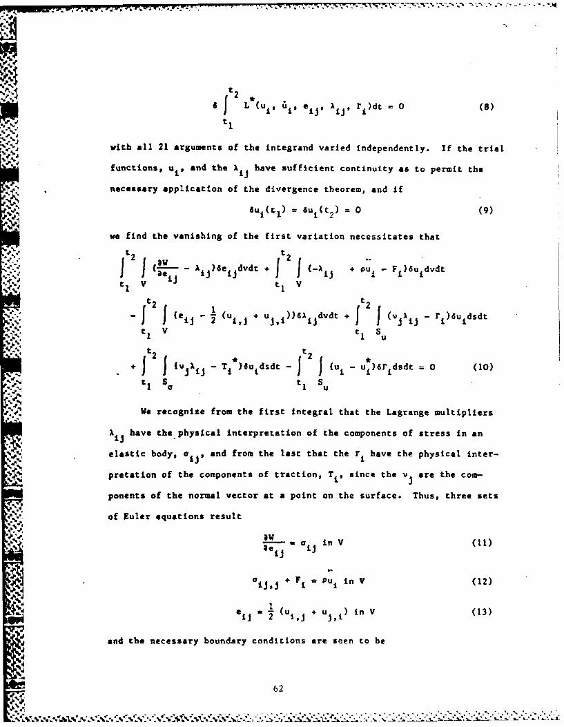
:':) ,t2a J L*(u,, u, ej' ij' r)dt 0 (8)

t

- Jwith all 21 arguments of the integrand varied independently. If the trial

functions, u,, and the XIJ have sufficient continuity as to permit the

. necessary application of the divergence theorem, and ifu (t au( 0 (9)

Iui(t =I) ui(t2 )

we find the vanishing of the first variation necessitates that

t 2 t"J - lI )6e dvdt + {- J + Pui- F )6u dvdt

-, ti Vst2 t2t'" (ei1 - 1 (u,,j + uJ, )J6X1Jdvdt + t I (V XiJ - r,)6u dsdt

t 1 V tI S

*"-" 2 J( I - )uds t 2

+, 2 I IV A - T *,)afo dsdt - t j ,. - u,}6r dsdt = 0 (10)t t I S t I S

We recognize from the first integral that the Lagrange multipliers

IiJ have the. physical interpretation of the components of stress in an

elastic body, oj, and from the last that the r have the physical inter-

pretation of the components of traction, T,, since the v are the com-

ponents of the normal vector at a point on the surface. Thus, three sets

of Euler equations result

3e a Oi in V (11)

+ F +IM Pu i in V (12)

e (u + u )in V (13)ij 2 ijJ ji

and the necessary boundary conditions are seen to be

.6~62

T 1 .v oi on S Su 4- S+a (14)

T - T on S (15)

S.-u * on S (16)

Since these are the field equations and boundary conditions of

elastodynamics, we conclude that the proposed extension is appropriate,

whether it be viewed as a relaxation of the class of functions to be used

with Hamilton's principle, or as an extension of Reissner'a principle to

other than simple harmonic motions. Equation 10, it should be noted,

is included in the further generalization due to Yu6 . This dynamic

variational principle differs from that of Dean and Plass 7 in that

Su need not vanish on S

4U.

463

,-

i:i.0d'|

a.

3I. An Approximate Method

Our interest here, of course, is not in deriving once again the

equations of elastodynamics, but rather in developing a procedure whereby

approximate solutions can be obtained for otherwise intractable problems.

To do this, we return to equation 10 and make use of the identification

that the Lagrange multipliers are, in fact, stresses and tractions.

We are interested in the class of problems for which a number of

solutions to the field equations are readily obtained, but for which dif-

ficulties in obtaining solutions arise because of mixed boundary conditions

in the form of Equations 15 and 16. We assume that a large number, N, of

systems of stresses, oij , and displacements u n, can be found, and that

each system satisfies Equation 12, and further, that these stresses sat-

isfy an elastic constitutive relationship, Equation 11, together with

strains e which are derived, through Equation 13, from the displacements,uln

U * We then take as trial functions the superpositions of such solutions,II

orN

a j(x,t) = I an aijn(x,t) (17)n=l

andN

ui(x,t) I a nu In(Xt) (18)n=l

It follows that every such trial function will also satisfy the system

field equations, 11-13. Tractions, Ti, may be constructed from these

stresses so as to satisfy Equation 14 on each point of S.

For such trial functions, all but the last two integrals of Equation

10 are zero identically. The variational principle has thus led to the

requirement that

64

t t2

4n -

I)TT a dd u )6T dsdt 0 (19)

SO t1 Su

From condition, we propose to construct an algorithm for determining

the set of coefficients an which, for any N selected, leads to the best

approximate solutions in the form of equations 17 and 18. The most general

arbitrary variation within the space spanned by these N solutions may also

be written as an expansion of these same N solutions, or

N,o I da a mo (x,t) (20)

4/) m=l mu

dul =I 6amuim(xt) (21)M=l

Substituting these and Equations 17 and 18 into equation 19 leads to a

single equation. Since the variation must be arbitrary, however, any con-

venient choice of coefficients, 6am may be made. It Is particularly con-

venient to make the selection:

Ga 0 for m p, m = ,N (22)

Ba = I for m= p, p = lN (23)

so as to obtain a system of N equations for the N coefficients an or

*N t 2

n= 1 wi~ud J i I I1~ o * 1d

1 0u (24)

t2

T-uId u, vjaj pds)dt'• 1 ( Ti u1 ds - u 1 i~

t Sa SU

For any given boundary conditions, T a I nd ui , and for any selected set

of solutions to the field equations, the an may be found and the approximate

solution determined. It has been previously found 8 that static problems

with mixed boundary conditions may be successfully treated in a similar

65

%JVO~

*'&* ~ ~ . . *'.% 4-.. V '..'~.v;-v -. - '~ V ~ ' C . ~ -

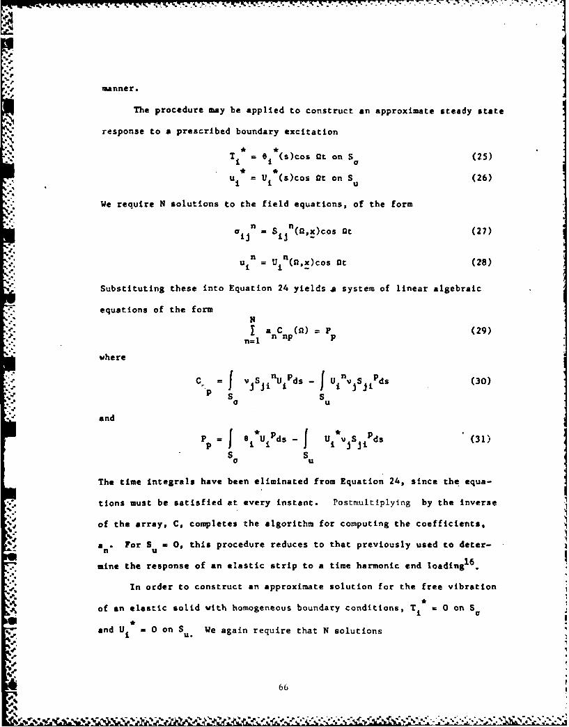
manner.

The procedure may be applied to construct an approximate steady state

response to a prescribed boundary excitation

T1 = 1 (s)cos At on S (25)

ui = U (s)cos at on S (26)

We require N solutions to the field equations, of the form

aij = Sijn(Qix)cos at (27)

n

U = Utn(n,x)cos At (28)-a. i

Substituting these into Equation 24 yields . system of linear algebraic

equations of the formNI a C (a) =P (29)

n=l p

where

C.p =1 S IjisUiPds- J uinVjs i p ds (30)

S o Sa U

-S and

P= f * UjPds-f * vS Pds (31)

S0 Sff U

The time integrals have been eliminated from Equation 24, since the equa-

tions must be satisfied at every instant. Postmultiplylng by the inverse

% of the array, C, completes the algorithm for computing the coefficients,

a . For S = , this procedure reduces to that previously used to deter-n U

mine the response of an elastic strip to a time harmonic end loading16.

In order to construct an approximate solution for the free vibration

of an elastic solid with homogeneous boundary conditions, Ti 0 on S

and U on S. We again require that N solutions

4U

66

n n

i %ii

.' S. n ij w,x)cos

Ui~n un(,U. ( ,X)cos Wt (33)

be available. Here, the natural frequency, w, is to be determined. Equa-

tion 24 now reduces to a set of homogeneous algebraic equations

NC (W)-=O0 (34)

-.- : n=1 i

with Cnp given by Equation 30. Estimates of natural frequencies, w, arise

from setting

det(C)= 0 (35)np

and the corresponding mode shapes may be determined by returning the re-

suiting value of w to Equation 34 and computing ratios of coefficients.

We have now completed the development of a procedure whereby approx-

imations to the forced response of elastic solids to time harmonic boundary

excitations may be obtained. Approximations to the natural frequencies

and the corresponding mode shapes may also be developed, even for objects

of complex geometry. If the available set of solutions can be shown to

be complete, convergence to an exact answer is to be expected in both cases.

If the available set of solutions is merely "large", only an approximazAon

can be anticipated.

467

".-4 . -.. . -. -. .. -, , .

1ll. Summary

A new variational principle has been developed and used to develop a

general approach to the problem of determining the frequencies and mode shapes

of freely vibrating elastic systems. Specific results from an application to

9,10the vibration of membranes have been given elsewhere .These results may,

of course, be immediately transferred to other physical systems having the same

differential equation and boundary conditions, such as the waveguide. More

recently, the method has been applied to the determination of the mode shapes

and natural frequencies of vibrating plates. Specifically, the problem con-

sidered was the circular plate, clamped on a portion of the edge and free on

the remainder Even though the solution algorithm requires finding, by

iteration, the values of a parameter which zero the determinant of a large

matrix, the computation time required was found to be substantially less than

that required to obtain similar results by using the method of finite elements.

68

References

1. Fund, Y. C., Foundations of Solid Mechanics, Prentice Hall, 1965, p 399.

2. Reissner, E.,"On a Variational Theorem in Elasticity", Journal of Math. andPhys., Vol XXIX 1950, pp 90-95.

3. Reissner, E.,"On Variational Principles in Elasticity", Calculus ofVariations and Its Applications, Proc. Sym. on Calculus of Variations,Vol VIII, American Math Soc, McGraw-Hill, 1958, pp 1-6.

4. Plass, H. J., Jr., J. H. Gaines, and C. D. Newsom, "Application of Reissner'sVariational Principle to Contilever Plate Deflection and Vibration Problems",Journal of Applied Mechanics, Vol 29, March 1962, pp 127-135.

5. Washizu, K., Variational Methods in Elasticity and Plasticity, PergamonPress, Oxford, 1968, pp 31-34.

6. Yu, Y. Y.,"Generalized Hamilton's Principle and Variational Equation of

Motion in Nonlinear Elasticity with Application to Plate Theory", J. ofAcoustical Society of America, Vol 36, No. 1, January 1964.

7. Dean, T. S. and Plass, H. J., "A Dynamic Variational Principle for ElasticBodies and Its Application to Approximation in Vibration Problems",

Development in Mechanics, Vol 3, No. 2, Proc. 19th Midwest Mechanics Conf,1965, pp 107-118.

9. Van Sickel, J. R., Jr., Vibrations of Membranes and Plates with MixedBoundary Conditions, M.S. Thesis, Air Force Institute of Technology,Wright-Patterson AFB OH, December 1978.

10. Torvik, P. J. and Van Sickel, "Natural Frequencies of Membranes HavingMixed Boundary Conditions" presented at the 95th Meeting of the AcousticalSociety of America, Providence RI, May 1978.

11. Torvik, P. J., "A Variational Approach to the Dynamics of Structures HavingMixed or Discontinuous Boundary Conditions", Manuscript in preparation.

69

9'f , ,V , ' ., ' ,. ., ; ' ' '; ' .. 4 . ,. .: -. ' . ', '. .: ., .'. - " " -1 . - o "-'-" ." " - " '

-V . u . .. 77. . . .. .

THE VALIDITY OF LINEAR VELOCITY CALCULATIONS

OF LOW PRESSURE GAS FLOWS IN A FLOW TUBE

P. J. Wolf and E. A. Dorkoij

Department of PhysicsAir Force Institute of Technology

* Wright-Patterson Air Force Base, Ohio 45433

and

S. J. Davis

Air Force Weapons LaboratoryKirtland Air Force Base, New Mexico 87117

ABSTRACT

The linear velocity and velocity profile of argon flowing

in a flow tube were determined experimentally by use of a

luminosity time-of-flight technique. The experiment can serve

V. as a simple introduction to flow tubes and to velocity profile

determinations in a physics or fluid mechanics laboratory. The

experiment allowed the observation of a laminar flow and a com-

parison of linear velocity calculated from plug flow considera-

tions with the linear, centerline velocity determined experimn-

tally. It ws found that the linear velocity was 1.62 times the

plug flow (average) velocity at a flow rate of 4576.0 standard

cc/min and 1.77 times the plug flow velocity at 5262.4 standard

cc/min. The velocity results were compared with those predicted

by the Poiseuille flow formula which governs ideal, fully developed

internal flows.

INTRODUCTION

Flow tubes are relatively simple devices which can be used

to determine the rates of fast reactions, to generate excited

chemical species, and to study the rates of decay of the emissions

from excited species. These studies can be accomplished because

in the flowing gas, little mixing occurs between reactants enter-

ing anr' products leaving the tube. The determinations of the

mechanism and kinetics of a large number of fast reactions at

70

temp~eratures below 1000 K have been done in this manner [In2

addition, with improvements in flow tube systems, high temperature

reactions occurring in such systems as FeO (31 and Al /0 (4] have2 2been studiied. Other applications of flow tubes have been report-e d [ 5 , 8 ]

In or~der to perform meaningful experiments, the linear velo-

cities of the flowing gases mujst be determined accurately. Linearvelocities have been reported in many of the published studies [,8These velocities were needed to calculate reaction rates andi to

provide a basis for a correlation between various physical para-

meters. In general, the velocities were calculated using the plug

flow assumption [8-101. Plug flow is defined as an idealized state

of flow such that, over any cross-section perpendicular to the

fluid motion, the mass flow rate and the fluid properties, P, T,and p,, remain constant. Extensive information is lacking concern-

ing the validity of the plug flow assumiption in flow tube applica-

tions where the pressure is low (4 - 10 Torr), buxt where-the flow

is still in the viscous flow regim. Swearengen [1)and Armstrong

and Davis l2 have reported limited results on this problem,

although it was not a main concern of their studies. The current, .~.work was conducted to develop a simple experimental method to de-

tail the validity of the plug flow assu~mption in the calculation

of the linear velocity of a low pressure gas in a flow tube. The

linear velocity was determined experimentally and compared to cal-

culations based on the plug flow assumption. En addition, the

velocity profile was studlied to determine possible deviations fromn

plug flow. The experimental apparatus which was utilized and the

technique for measuring the velocity profile are simple enough so

v that they could be used as a laboratory experiment in a physicsor fluid flow laboratory. The experiment could introduce the stu-

dents to the use of flow tubes and also could serve as a simple

method of obtaining the velocity profile for a gas in laminar

flow. The equipment is inexpensive and simple to operate, yet theN results give a good approximation of the theoretical parabolic

71

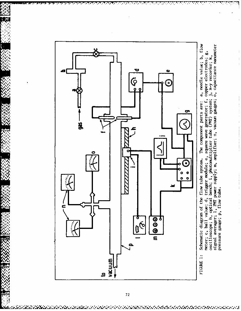
-. Frlr7 p 17- W Y 1. !.b, 4

> uO 0

( -A J - 4

a) I)s.

0.

U) W (n

) 4 .aAJ-44-

4-1C

tro

-4-

00

000

04

00 C

C-4

72

velocity profile to be expected under the experimental conditions.

While standard techniques, such as pitot tubes and hotwire

anemometers[13, 14] have been used in the past for velocity pro-

file measurements, the present experiment utilized a luminosity

time-of-flight technique.A stream of argon gas was excited in a high voltage discharge

in the flow tube, near the entrance. The time-of-flight of the

luminous argon was determined at a series of stations downstream

of the discharge by detection of the visible emission of the

excited argon. The linear velocity of the flowing gas was calcu-

lated from these data. The advantage of this technique for a

laboratory envirorment is the simplicity of the approach. Once

"" 'the apparatus is assembled, simple movement of the detector along

an optical bench is the only adjustment which needs to be made.

By traversing the detector perpendicular to the direction of gas

flow at various stations downstream at the flow tube, the develop-

ment of the profile can be observed.

EXPERIMErAL SECTION

The flow tube arrangement utilized in this experiment was

based on the system described by Swearengen, Davis and

Niemczyk 7, 1. It is shown schematically in Figure 1. The flow

tube was composed of sections of thick-alled pyrex glass tubing

5.1 cm I.D. joined together to form a system 162 cm in length.

The tube consisted of a gas injection region, a discharge region

and a test region. It was supported on an aluminum stand.

A gas flow system furnished the flow tube with a continuous

supply of high purity argon (99.98%). Since the volumetric flow

rate was required in order to calculate the theoretical linear

velocity of the gas, this flow rate was measured using a Hastings

Model All-I1K Linear Mass Flowmeter. The flow rate was controlled

by a Jamesbury ball valve placed downstream from the flowmeter.

The gas entered the tube in the injection region. This 31 an

'4 length of the flow tube, located directly upstream of the discharge

.73

region, was provided in order to obtain a reattached flow of gas

prior to entry into the discharge region. Provision for the gas

flow to become reattached in the flow tube becomes important when

the gas feed line diameter is different from the flow tube dia-

meter. That is, when gas is sudenly expanded as it enters a tube,

a jet stream develops. Therefore, it is necessary to find a dis-

tance downstream from the inlet hole where the flow becomes re-

attached. In the present study, the flow tube diameter was 5.1 cm

and the inlet hole diameter was 1.3 cm. For this configuration,

the recirculation zone length was found to be 15 cm[ 1 5 ] A section

of tube approximately twice this length was used to serve as the

injection region.

Once reattached flow was achieved, the gas entered the dis-

charge region. A portion of the argon flowing between copperelectrodes was ionized and excited into metastable electronic

states. These states continued to emit detectable visible radia-

tion for a considerable distance downstream, and this emission

(or afterglow) served as the basis for the velocity determinations.

The discharge region was constructed with a pyrex glasscross, 20 cm in length. The cross was located directly downstreamof the gas injection region. Copper electrodes, 0.32 cm in dia-

meter, were inserted in the cross arms through 1.3 cm thich plexi-

glass plates. The electrodes were adjusted to provide a 1.0 cmgap perpendicular to the flow tube centerline. A high voltage arc

was produced between the electrodes with an EGSG Model TH-II 30 kv

trigger module. A repetitive, pulsed discharge was achieved with

a 2 Hz, 20 v peak-to-peak square wave from a Wavetek Model IVA5pvoltage controlled generator.

V. The observation section of the test region of the flow tube,

61 an in length, was placed directly downstream of the discharge

region. An optical bench was positioned alongside this portion of

the tube. The bench contained a scale graduated in cm to measuredistances from the electrode to the observation point. A IP21

photmiltiplier tube (PMT), used to detect the radiation from the

74

argon afterglow, was moumted on the optical bench. A variable

slit, adjusted to a width of 0.2 cm, was placed in front of the

PMr. An iris, adjusted to give a diameter of 1 an, was placed in

front of the slit. The iris allowed the photomultiplier tube to

sample the radiation at different heights in the flow.

The output of the PMr was fed into a Keithly Model 427 cur-

rent amplifier. The signal was then sent into a Princeton Applied

Research Model TDH-9 Waveform Eductor (signal averager). Approxi-

mately 100 signals were averaged. The signal averager was trig-

gered by the signal from the square wave generator.. Therefore,

the signal averager accepted signals only when the discharge was

triggered. The averaged signal was then sent into a Hewlett-

Packard Model 7045a X-Y Recorder. The recorder produced a curve

of relative intensity vs time.

A 20 an long pyrex glass tee was used in the test section

following the observation area. This tee housed the pressure

and vacuum gauges. Hastings DV-4D and DV-6 vactum gauges were

used to measure vacuun. Pressure during gas flow measured witha capacitance manometer device (MKS Baratron Type 77 Pressure

Meter).

Two Welsh 17.7 CFM mechanical vactum pumps were used to re-

duce the pressure in the flow tube. A pressure of 50 microns was

achieved with no gas flow. A ball valve, used to retard the gas

flow to provide a higher gas pressure with no change in flow rate,

was placed in the line betwen the pumps and the flow tube.

RESULTS

A. Linear Velocity

The linear velocity of the flowing argon gas was experimen-

tally determined at various gas pressures and flow rates by de-

tecting the afterglow from the excited argon with the PM. For

these measurements, the PMr was positioned at various stations

downstream of the electrodes. The height of the PMr system was

adjusted such that a signal was detected from the flow tube center-

75

line. The pressures, flow rates and downstream station distances

for which linear velocities were calculated are listed in Table 1.

The centerline signal from the flow tube was determined by travers-

ing the PMT and the iris vertically at each station until the fast-

est time-of-flight of the glowing gas was obtained.

Data gathered during this operation included the distance (X)

of the PMT station downstream of the electrodes and the time (t)

at which the PMT detected the leading edge of the emission of the

argon afterglow. An adjustment was made in the value of X in order

to correct for the self-diffusion of the glowin argon. The square

root of the mean square distance diffused, TX23, was calculated

using Eq (1)[16, 17]

TX2 -7

% = /2Dt (1)

where D is the diffusion coefficient of argon and t is the time-

of-flight of the gas to each station. The correction amounted to

less than 4% of the total distance traversed.

The linear velocity of argon was calculated by performing a

linear regression analysis on the data. A linear least squares

fit was ccmputed by regressing t on X. Plots of t vs X were con-

structed along with the lines representing the results of the

least squares analyses. This information is shown in Figure 2.

The linear velocities of the gas flows were determined by invert-ing the slopes of the lines. The results are shown in Table II,

along with the plug flow velocity calculations.

. Pf = 1.43Q P(ATM)/60 P(GAS) A cm/sec (2)

where Q is the volumetric flow rate in standard cc/min of air, 1.43

is the conversion factor for the Hastings Mass Flowmeter to convert

Q into the volumetric flow rate of argon, P(ATM) is the atomspheric

pressure in torr, P(GAS) is the flowing gas pressure in torr, A is

76

.- ,

f,...

TABLE I

EIMHE2JTAL PARAMERS FOR LINEAR VELOCIIY DUrERMINATIONS

x (cm) , p (torr) v (std cc/min)

16.9 4.2 4576.06.0 4576.0

26.9 4.2 4576.0

5.0 5262.4

6.0 4576.0

[0.1 5262.4

31.9 5.0 5262.4

10.1 5262.4

33.9 10.1 5262.437.1 4.2 4576.0

5.0 5262.4

6.0 4576.0

42.1 5.0 5262.4

47.0 4.2 4576.0

5.0 5262.4

6.0 4576.0

.,\ .52.0 5.0 5262.4

56.9 5.0 5262.4

" 57.4 4.2 4576.0

6.0 4576.0

77

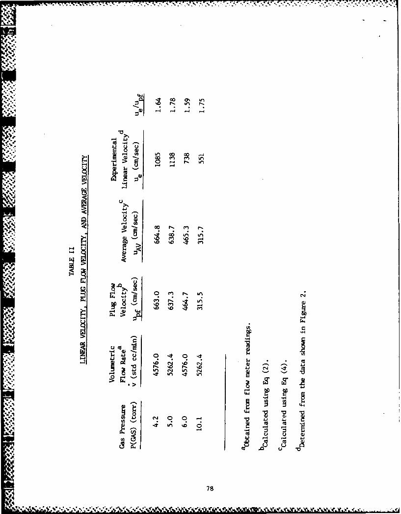
%v

% .11

-4 c

-4 -4

-4 ~ -4-

4,1

>

0 4J...

Cu V

aLeao-S4

*%'. •

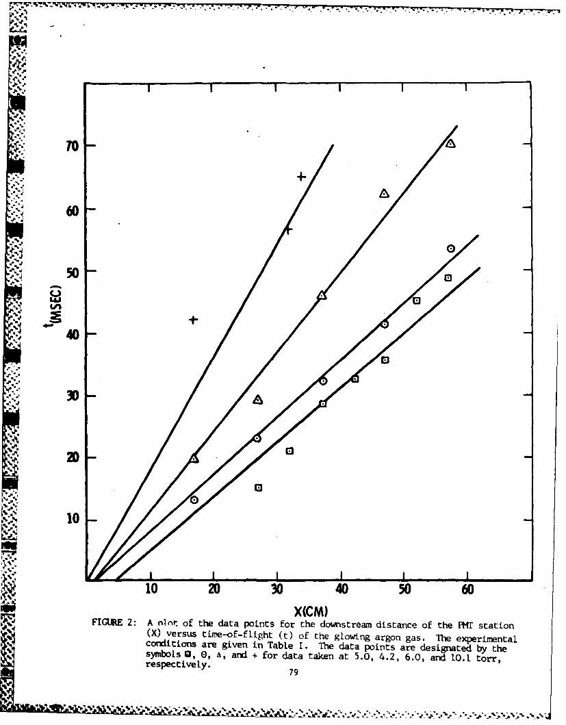
-.-. ~ *4. -,- 4 . -

70

60

50 0

, '...

V..V

*440

30

10

10 20 30 40 (0 0

~X(CM),_ FIGURE 2: A nlnt of the data points for the downstream distance of the PMr station

(X) versus time-of-flight (t) of the glowing argon gas. The experimentalConditions are given in Table I. The data points are designated by thesymbols 0, 0, A, and + for data taken at 5.0, 4.2, 6.0, and 10.1 tort,respectively.

7

790

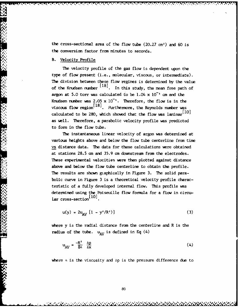
. 7

the cross-sectional area of the flow tube (20.27 cm2) and 60 is

the conversion factor from minutes to seconds.

B. Velocity Profile

The velocity profile of the gas flow is dependent upon the

type of flow present (i.e., molecular, viscous, or intermediate).

The division between these flow regimes is determined by the valueof the Knudsen number [l8]. In this study, the mean free path of

argon at 5.0 torr was calculated to be 1.04 x 10' cm and the

Knudsen number was 2.05 x 107'. Therefore, the flow is in the

viscous flow region[ 8 . Furthermore, the Reynolds number was[10]calculated to be 280, which showed that the flow was laminar

as well. Therefore, a parabolic velocity profile was predicted

to form in the flow tube.

The instantaneous linear velocity of argon was determined at

various heights above and below the flow tube centerline from time

vs distance data. The data for these calculations were obtained

at stations 28.5 cm and 35.9 an downstream from the electrodes.

These experimental velocities were then plotted against distance

above and below the flow tube centerline to obtain the profile.The results are shown giaphically in Figure 3. The solid para-

bolic curve in Figure 3 is a theoretical velocity profile charac-

teristic of a fully developed internal flow. This profile was

determined using the Poiseuille flow formula for a flow in circu-

lar cross-section[ 10O].

u(y) = 2uAV [1 - y2 /R')] (3)

where y is the radial distance from the centerline and R is the

radius of the tube. uAV is defined in Eq (4)

-I p( 4 )uAV = 8n Ax

where n is the viscosity and Ap is the pressure difference due to

80

202

-10+

-20

FICLRE 3: Experimental andi theoretical velocity profiles at 5.0 torr. Thie parabolic

profile was calculated using the Poiseuille flow formula. The experimentaldata were taken at Pr~f stations 28.5 cm ()andi 35.9 cn (0) dow'nstream ofthe electrodes.

I 4N

81

-. ,..~ - ~ .. .r .-. . ° -- °.o o o- .4

k. .. , . . . . . . .. .. - . - . .. . .

viscous forces over a length of tube Ax. If the pressure at one

end of the tube is known, then the pressure at the other end can

be calculated from Eq (5)[2]

- P 2 = 16F' Ln RoT/nR4 (5)

where F' is the flow rate in moles/sec, L is the length of the

tube, Ro is the universal gas constant, and T is the absolute

temperature. For example, using for the viscosity of argon223.7 x 1076 poise at 296 K, a P1 of 10.1 torr and a flow rate

of 3.62 x 1O-0 mole/sec, the pressure difference due to viscousforces was calculated to be 1.09 x lO-' torr.

The experimental velocity profiles in Figure 3 revealed an

approximately parabolic configuration at both stations. While

the profile obtained at 35.9 cm downstream slightly more closely

resembled the theoretical curve than the profile at 28.5 cm, the

difference in the profiles is within experimental scatter. There-

fore, the flow was considered fully developed at both downstream

stations. The characteristic length for an internal flow to be-

came fully developed was calculated using Eq (6)[9]

X=03(R)D (6)

where XL is the characteristic length, Re is the Reynolds number

and D is the tube diameter. The laminar development length was

calculated as 42.7 cm from the point where the flow became reat-

tached at the inlet region. Thus, the flow was fully developed

at 16.7 an downstream from the electrodes. This simple calcula-

tion was strongly supported by a numerical calculation for the

same system which was performed by Rapagnani and Davis[191

DISCUSSION

The velocity profiles of the flowing argon gas at various low

pressures were parabolic. Thi s result indicates that a fully

82

developed laminar flow was present throughout the experiment.

Based on this conclusion, a comnparison can be made between theexperimentally determined values for plug flow (Eq (2)) and the

average velocities calculated by the use of Eqs (4) and (5).These values are reported in Table II. The correspondence betweenvalues shows that the plug flow velocity can be used as the average

velocity in calculations for flow tubes when low pressure laminarflow is occurring.

The results of the linear velocity calculation along theflow tube centerline should be twice the average or plug flow

velocity in the ideal case. This is evident when y is set equal

to 0 in Eq (3). A canparison between the experimental linear

velocity results at y = 0, (ue), and the plug flow values showsthat the factor of 2 is being approached, but experimentally the

linear velocity is somnewhat slower than predicted by theory. The

discrepancy can be the result of a number of factors. Plug flow

calculations do not take into account frictional effects, since

this calculation is based on an ideal flow. In this study, the-. .,*flow experienced frictional effects due to shearing stresses and

pressure losses which caused the deviation from plug flow. Also,

in the present case the frictional effects were increased when the

gas flowed past the electrodes.Based on these studlies, it is concluded that a calculation of

centerline velocity based on a laminar velocity profile gives a

much better value than a calculation based on plug flow. If

perturbations to the flow are slight, as in the present case, a

correction factor of 1.6 - 1.7 applied to the plug flow value will

give a good estimate of the centerline flow velocity.

di 83

-REFRNES

1. G. Porter, Ed., Progress in Reaction Kinetics, Vol 1, Pergamon

v: Pres, New York, 1961.

2. B. A. Thrush, Science, 154, 477 (1967).

3. A. Fontjin and S. C. Kurzius, Chem. Phys. Letters, 13, 507(1972).

4. A. Fontjin, W. Felder, and J. J. Houghton, Chem. Phys. Letters,27, 365 (1974).

5. R. L. Brown, J. of Res., NBS, 83 1 (1978).

6. G. Dixon-Lewis, W. E. Wilson, and A. A. Westenberg, J. Chem.Phys., 44, 2877 (1966).

7. P. M. Swearengen, S. J. Davis, and T. M. Niemczyk, Chem. Phys.Letters, 55, 274 (1978).

8. S. M. Walas, Reaction Kinetics for Chemical Reactions, McGraw-Hill Book Company, Inc., New York, 1959.

9. J. M. Coulson and J. F. Richardson, Chemical Engineering, Vol 3,Pergamon Press, New York, 1971.

10. K. Denbigh, Chemical Reactor TheoryX An Introduction, CambridgeUniversity Press, New York, 1965.

11. P. M. Swearengen, "Kinetic Studies of Silicon and GermaniumOxide Reactions", PhD Dissertation, Department of Chemistry,The University of New Mexico, December 1977.

12. R. A. Davis and S. J. Armstrong, Chem. Phys. Letters, 57, 446(1978).

13. C. F. Shoop, and G. L. Tuve, Mechanical Engineering Practice,5th Edition, McGraw-Hill Book Company, Inc., New York, 1956.

14. J. E. A. John, and W. Haberman, Introduction to Fluid Mechanics,Prentice-Hall, Inc., Englewood Cliffs, N. J., 1971.

15. M. A. Penrucci, '"arametric Evaluation of Total Pressure Lossand Recirculation - Zone Length in a Sudden Expansion Ccmbustor",M.S. Thesis, School of Engineering, Air Force Institute ofTechnology, Wright-Patterson Air Force Base CH 45433, 1974.

16. W. J. Moore, Physical Chemistry, 4th Edition, Prentice-Hall,Inc., Englewood Cliffs, N. J., 1972, pp 162-163.

84

J. U.,. **.*S.

V. - .1.-*i

N;.,

17. Shyh Wang, Solid State Electronics, McGraw-Hill Book Company,Inc., New York 1966, pp 282-290.

18. A. Roth, Vacuum Technolog, North-Holland Publishing Co.,New York, 176.

19. N. L. Rapagnani and S. J. Davis, Chemical Laser Branch, AirForce Weapons Laboratory, Albuquerque NM, private conruication.

oo,8

-'I.

UnclassifiedSECURITY CLASSIFICATION OF THIS PAGE

REPORT DOCUMENTATION PAGE1. REPORT SECURITY CLASSIFICATION lb. RESTRICTIVE MARKINGS

Unclassified2a. SECURITY CLASSIFICATION AUTHORITY 3. DISTRI BUTION/AVAI LABILITY OF REPORT

Approved for public release; distribution2b. DECLASSIFICATION/DOWNGRADING SCHEDULE unlimited.

4. PERFORMING ORGANIZATION REPORT NUMBER(S) 5. MONITORING ORGANIZATION REPORT NUMBER(S)

AFIT-EN-TM-84-1. NAME OF PERFORMING ORGANIZATION b. OFFICE SYMBOL 7a. NAME OF MONITORING ORGANIZATION

Air Force Institute of Techno l gfappicble)

School of Engineering AFIT/EN6c. ADDRESS (City, State and ZIP Code) 7b. ADDRESS (City, State and ZIP Code)

Wright-Patterson AFB OH 45433

Ba. NAME OF FUNDING/SPONSORING Sb. OFFICE SYMBOL 9. PROCUREMENT INSTRUMENT IDENTIFICATION NUMBERORGANIZATION (If applicabie)

Sc. ADDRESS (City. State and ZIP Code) 10. SOURCE OF FUNDING NOS.

PROGRAM PROJECT TASK WORK UNITELEMENT NO. NO. NO. NO.

11. TITLE (Include Security Classification) A Festschrift ofTechnical Papers Presented to W. S. Ericksen U)

12. PERSONAL AUTHOR(S)

Brian W. Woodruff, Ca t, USAF: editor - see item 19 for authors of papers13. TYPE OF REPORT 13b. TIME COVERED 14. DATE OF REPORT (Yr., Mo., Day) 15. PAGE COUNT

Technical Memorandum FROM TO 1984 January 8716. SUPPLEMENTARY NOTATION Ap roved lor ptic releaze: IAW AFE 190.17.

Dean lot Resarch and Protesstonn! ^

17. COSATI CODES 18. SUBJECT TERMS (Continue on reverse if neceeefrp [tfeA QUW& (ATC)FIELD GROUP SUB. GR. all It 4,43

I Key words - see reverse.

19. ABSTRACT (Continue on reverse if necessary and identify by block number)This volume contains eight technical papers written by colleagues of Wilhelm Ericksen inhonor of his 30 years of service on the faculty of the Air Force Institute of Technology.The following is a list of titles and authors of the papers in the volume: "The PCTControl System Design for Sampled-Data Control Systems", by C. H. Houpis; "Asymptotic Non-Null Distribution of a Test of Equality of Exponential Populations", by R. W. Kulp andB. N. Nagarsenker; "Irrotational and Solenoidal Waves in General Coordinates", by D. A. Lee;"Some Problems of Estimation When Some Prior Information is Available", by A. H. Moore;"Non-Null Distributions of the Likelihood Ratio Criterion for the SpectralMatrix of aGaussian Multivariate Time Series", by B. N. Nagarsenker; "Probability of Destruction ofa Point Target in Space", by J. S. Przemieniecki; "A New Variational Principle for Elasto-dynamic Problems with Mixed Boundary Conditions", by P. J. Torvik; "The Validity of LinearVelocity Calculations of Low Pressure Gas Flows in a Flow Tube", by P. J. Wolf, E. A.Dorko and S. J. Davis.

20. DISTRISUTION/AVAILABILITY OF ABSTRACT 21. ABSTRACT SECURITY CLASSIFICATION

UNCLASSIFIEDIUNLIMITED CM SAME AS RPT. 99 DTIC USERS 0 Unclassified

22s. NAME OF RESPONSIBLE INDIVIDUAL 22b. TELEPHONE NUMBER 22c. OFFICE SYMBOL(Include Apro Code)

Brian W. Woodruff 513-255-2915 AFIT/ENC

00 FORM 1473, 83 APR EDITION OF 1 JAN 73 IS OBSOLETE. UnclassifiedA SECURITY CLASSIFICATION OF THIS PAGE

".. ........................................................,.. r,... ........,. .................. .............-.. ,-..... ....-.. ... . -..-

S. . . . . . . . . .

linr 'n ~cfi Pd

SECURIT Y CLASSIFICATION OF THIS PAGE

.tei- A continued:

pseudo-continuous-time control systemsamples-data systemexponential populationslikelihood ratio criterionasymptotic non-null distributionChi-3quare distributionselastodynamic displacement fieldsirrotational wavessolenoidal wavesprior informationad-.-* 3ble estimators

inada.issible estimatorsspectral matrixmultivariate time seriestarget destruction probabilityspherical error probablecircular error probablelinear error probablevariational principleelastodynamic problemsboundary conditionsflow tubesplug flowPoiseuille flow formula

,

Unclassified

SECURITY CLASSIIeATION re% TWIR PAnPa

.. ~ - ~ -- r.- ~ - - ru

'0 "-'4 .' . p

-fit(41. 4

-Wa.

t

* . -~;;p~Pt [>' c [~ 7t 'i~!*~ *r -

-4 2 .~ ~ 'rat

* > a ~ ft'>'b A. fit

Ac ~vr%'% C ~1 ?~t#4t$~

4 r~ *t

,%P -a9, a, &

ft

4'

Cx' ?L}V - ~

f *'1~ A -

9~Ir.4, 0' .9

* - ' &t

[in'; '"~~~: A

3t1 / at.

j~ ! -a

6' ak -r 6~

.y 4a.a -. - a,-ra4ar.aa

''' 0?~?

-. 4. *tj 4tN

2rtt~#fflf9LA a a, $4 ~

t t'j4 ~

- - M.A -. I-Sbz9wa?~-DtkJAtM ~ tat' . *- ~ ~-

trw ~ -~vV -'

* 4$-~9qtt~ - a KfS f~L9.S5-... ~,ada. --

'-4' 'a-

a? a'42 ~ sit

c$.

S

lAy L-~t~.-

ada ,-, ~k#:<~ ~C

1~A: t:1,Ya * a . a 4

S...'?. *~L.. ~ s at. t,.,A~P - a-