sequential monte carlo - snu · nando de freitas & arnaud doucet ubc ( ) sequential monte carlo...
TRANSCRIPT

Sequential Monte Carlo
Nando de Freitas & Arnaud Doucet
University of British Columbia
December 2009

Tutorial overview• Introduction Nando – 10min
• Part I Arnaud – 50min
– Monte Carlo
– Sequential Monte Carlo
– Theoretical convergence
– Improved particle filters
– Online Bayesian parameter estimation
– Particle MCMC
– Smoothing
– Gradient based online parameter estimation
• Break 15min
• Part II NdF – 45 min
– Beyond state space models
– Eigenvalue problems
– Diffusion, protein folding & stochastic control
– Time-varying Pitman-Yor Processes
– SMC for static distributions
– Boltzmann distributions & ABC
20th century

SMC in this community
• Michael Isard and Andrew Blake popularized the method with their
Condensation algorithm for image tracking.
• Soon after, Daphne Koller, Stuart Russell, Kevin Murphy, Sebastian Thrun,
Dieter Fox and Frank Dellaert and their colleagues demonstrated the method
in AI and robotics.
• Tom Griffiths and colleagues have studied SMC methods in cognitive
psychology.
Many researchers in the NIPS community have contributed to the
field of Sequential Monte Carlo over the last decade.

The 20th century - Tracking
[Michael Isard & Andrew Blake (1996)]

The 20th century - Tracking
[Boosted particle filter of Kenji Okuma, Jim Little & David Lowe]

The 20th century – State estimation
http://www.cs.washington.edu/ai/Mobile_Robotics/mcl/[Dieter Fox]

http://www.cs.washington.edu/ai/Mobile_Robotics/mcl/[Dieter Fox]
The 20th century – State estimation

The 20th century – State estimation

The 20th century – The birth
[Metropolis and Ulam, 1949]

Tutorial overview• Introduction Nando – 10min
• Part I Arnaud – 50min
– Monte Carlo
– Sequential Monte Carlo
– Theoretical convergence
– Improved particle filters
– Online Bayesian parameter estimation
– Particle MCMC
– Smoothing
– Gradient based online parameter estimation
• Break 15min
• Part II NdF – 45 min
– Beyond state space models
– Eigenvalue problems
– Diffusion, protein folding & stochastic control
– Time-varying Pitman-Yor Processes
– SMC for static distributions
– Boltzmann distributions & ABC

Arnaud’s slides will go here

Sequential Monte Carlo Methods
Nando De Freitas & Arnaud DoucetUBC
Nando De Freitas & Arnaud Doucet UBC ( ) Sequential Monte Carlo Methods 1 / 39

State-Space Models
fXkgk�1 hidden X -valued Markov process with
X1 � µ (x1) and Xk j (Xk�1 = xk�1) � f (xk j xk�1) .
fYkgk�1 observed Y-valued process with observations conditionallyindependent given fXkgk�1 with
Yk j (Xk = xk ) � g (yk j xk ) .
Main Objective: Estimate fXkgk�1 given fYkgk�1 online/o ine.
Nando De Freitas & Arnaud Doucet UBC ( ) Sequential Monte Carlo Methods 2 / 39

Inference in State-Space Models
Given observations y1:n := (y1, y2, . . . , yn), inference aboutX1:n := (X1, ...,Xn) relies on the posterior
p (x1:n j y1:n) =p (x1:n, y1:n)
p (y1:n)
where
p (x1:n, y1:n) = µ (x1)n
∏k=2
f (xk j xk�1)| {z }p(x1:n)
n
∏k=1
g (yk j xk )| {z }p( y1:n jx1:n)
,
p (y1:n) =Z� � �
Zp (x1:n, y1:n) dx1:n
We want to compute p (x1:n j y1:n) and p (y1:n) sequentially in time n.
For non-linear non-Gaussian models, numerical approximations arerequired.
Nando De Freitas & Arnaud Doucet UBC ( ) Sequential Monte Carlo Methods 3 / 39

Monte Carlo Methods
Assume you can generate X (i )1:n � p (x1:n j y1:n) where i = 1, ...,N thenMC approximation is
bp (x1:n j y1:n) =1N
N
∑i=1
δX (i )1:n(x1:n)
Integration is straightforwardZϕn (x1:n) bp (x1:n j y1:n) dx1:n =
1N
N
∑i=1
ϕn�X (i )1:n
�.
Marginalisation is straightforward
bp (xk j y1:n) =Z bp (xk j y1:n) dx1:k�1dxk+1:n =
1N
N
∑i=1
δX (i )k(xk )
Problem: Sampling from p (x1:n j y1:n) is impossible in general cases.
Nando De Freitas & Arnaud Doucet UBC ( ) Sequential Monte Carlo Methods 4 / 39

Basics of Sequential Monte Carlo Methods
Divide and conquer strategy: Break the problem of sampling fromp (x1:n j y1:n) into a collection of simpler subproblems. Firstapproximate p (x1j y1) at time 1, then p (x1:2j y1:2) at time 2 and soon.
Each target distribution is approximated by a cloud of randomsamples termed particles evolving according to importance samplingand resampling steps.
Nando De Freitas & Arnaud Doucet UBC ( ) Sequential Monte Carlo Methods 5 / 39

Importance Sampling
Assume you have at time n� 1
bp (x1:n�1j y1:n�1) =1N
N
∑i=1
δX (i )1:n�1
(x1:n�1) .
By sampling eX (i )n � f�xn jX (i )n�1
�and setting eX (i )1:n =
�X (i )1:n�1, eX (i )n �
then bp (x1:n j y1:n�1) =1N
N
∑i=1
δeX (i )1:n(x1:n) .
Our target at time n is
p (x1:n j y1:n) =g (yn j xn) p (x1:n j y1:n�1)Rg (yn j xn) p (x1:n j y1:n�1) dxn
so by substituting bp (x1:n j y1:n�1) to p (x1:n j y1:n�1) we obtain
ep (x1:n j y1:n) =N
∑i=1W (i )n δeX (i )1:n
(x1:n) , W(i )n ∝ g
�yn j eX (i )1:n
�.
Nando De Freitas & Arnaud Doucet UBC ( ) Sequential Monte Carlo Methods 6 / 39

Resampling
We have a �weighted�approximation ep (x1:n j y1:n) of p (x1:n j y1:n)
ep (x1:n j y1:n) =N
∑i=1W (i )n δeX (i )1:n
(x1:n) .
To obtain N samples X (i )1:n approximately distributed according top (x1:n j y1:n), we just resample
X (i )1:n � ep (x1:n j y1:n)
to obtain bp (x1:n j y1:n) =1N
N
∑i=1
δX (i )1:n(x1:n) .
Particles with high weights are copied multiples times, particles withlow weights die.
Nando De Freitas & Arnaud Doucet UBC ( ) Sequential Monte Carlo Methods 7 / 39

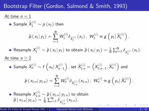
Bootstrap Filter (Gordon, Salmond & Smith, 1993)
At time n = 1
Sample eX (i )1 � µ (x1) then
ep (x1j y1) = N
∑i=1W (i )1 δeX (i )1 (x1) , W (i )
1 ∝ g�y1j eX (i )1 � .
Resample X (i )1 � ep (x1j y1) to obtain bp (x1j y1) = 1N ∑N
i=1 δX (i )1(x1).
At time n � 2
Sample eX (i )n � f�xn jX (i )n�1
�, set eX (i )1:n =
�X (i )1:n�1, eX (i )n � and
ep (x1:n j y1:n) =N
∑i=1W (i )n δeX (i )1:n
(x1:n) , W(i )n ∝ g
�yn j eX (i )n � .
Resample X (i )1:n � ep (x1:n j y1:n) to obtainbp (x1:n j y1:n) =1N ∑N
i=1 δX (i )1:n(x1:n).
Nando De Freitas & Arnaud Doucet UBC ( ) Sequential Monte Carlo Methods 8 / 39

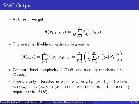
SMC Output
At time n, we get
bp (x1:n j y1:n) =1N
N
∑i=1
δX (i )1:n(x1:n) .
The marginal likelihood estimate is given by
bp (y1:n) =n
∏k=1
bp (yk j y1:k�1) =n
∏k=1
1N
N
∑i=1g�yk j eX (i )k �
!.
Computational complexity is O (N) and memory requirementsO (nN) .If we are only interested in p (xn j y1:n) or p ( sn (x1:n)j y1:n) wheresn (x1:n) = Ψn (xn, sn�1 (x1:n�1)) is �xed-dimensional then memoryrequirements O (N) .
Nando De Freitas & Arnaud Doucet UBC ( ) Sequential Monte Carlo Methods 9 / 39

SMC Output
At time n, we get
bp (x1:n j y1:n) =1N
N
∑i=1
δX (i )1:n(x1:n) .
The marginal likelihood estimate is given by
bp (y1:n) =n
∏k=1
bp (yk j y1:k�1) =n
∏k=1
1N
N
∑i=1g�yk j eX (i )k �
!.
Computational complexity is O (N) and memory requirementsO (nN) .
If we are only interested in p (xn j y1:n) or p ( sn (x1:n)j y1:n) wheresn (x1:n) = Ψn (xn, sn�1 (x1:n�1)) is �xed-dimensional then memoryrequirements O (N) .
Nando De Freitas & Arnaud Doucet UBC ( ) Sequential Monte Carlo Methods 9 / 39
SMC Output
At time n, we get
bp (x1:n j y1:n) =1N
N
∑i=1
δX (i )1:n(x1:n) .
The marginal likelihood estimate is given by
bp (y1:n) =n
∏k=1
bp (yk j y1:k�1) =n
∏k=1
1N
N
∑i=1g�yk j eX (i )k �
!.
Computational complexity is O (N) and memory requirementsO (nN) .If we are only interested in p (xn j y1:n) or p ( sn (x1:n)j y1:n) wheresn (x1:n) = Ψn (xn, sn�1 (x1:n�1)) is �xed-dimensional then memoryrequirements O (N) .
Nando De Freitas & Arnaud Doucet UBC ( ) Sequential Monte Carlo Methods 9 / 39

SMC on Path-Space - �gures by Olivier Capp·e
5 10 15 20 250.4
0.6
0.8
1
1.2
1.4
1.6
time index
stat
e
5 10 15 20 250.4
0.6
0.8
1
1.2
1.4
1.6
time index
stat
e
Figure: p (x1 j y1) and bE [X1 j y1 ] (top) and particle approximation of p (x1 j y1)(bottom)Nando De Freitas & Arnaud Doucet UBC ( ) Sequential Monte Carlo Methods 10 / 39

5 10 15 20 250.4
0.6
0.8
1
1.2
1.4
1.6
time index
stat
e
5 10 15 20 250.4
0.6
0.8
1
1.2
1.4
1.6
time index
stat
e
Figure: p (x1 j y1) , p (x2 j y1:2)and bE [X1 j y1 ] , bE [X2 j y1:2 ] (top) and particleapproximation of p (x1:2 j y1:2) (bottom)
Nando De Freitas & Arnaud Doucet UBC ( ) Sequential Monte Carlo Methods 11 / 39

5 10 15 20 250.4
0.6
0.8
1
1.2
1.4
1.6
time index
stat
e
5 10 15 20 250.4
0.6
0.8
1
1.2
1.4
1.6
time index
stat
e
Figure: p (xk j y1:k ) and bE [Xk j y1:k ] for k = 1, 2, 3 (top) and particleapproximation of p (x1:3 j y1:3) (bottom)
Nando De Freitas & Arnaud Doucet UBC ( ) Sequential Monte Carlo Methods 12 / 39

5 10 15 20 250.4
0.6
0.8
1
1.2
1.4
1.6
time index
stat
e
5 10 15 20 250.4
0.6
0.8
1
1.2
1.4
1.6
time index
stat
e
Figure: p (xk j y1:k ) and bE [Xk j y1:k ] for k = 1, ..., 10 (top) and particleapproximation of p (x1:10 j y1:10) (bottom)
Nando De Freitas & Arnaud Doucet UBC ( ) Sequential Monte Carlo Methods 13 / 39

5 10 15 20 250.4
0.6
0.8
1
1.2
1.4
1.6
time index
stat
e
5 10 15 20 250.4
0.6
0.8
1
1.2
1.4
1.6
time index
stat
e
Figure: p (xk j y1:k ) and bE [Xk j y1:k ] for k = 1, ..., 24 (top) and particleapproximation of p (x1:24 j y1:24) (bottom)
Nando De Freitas & Arnaud Doucet UBC ( ) Sequential Monte Carlo Methods 14 / 39

Illustration of the Degeneracy Problem
Degeneracy problem. For any N and any k, there exists n (k,N)such that for any n � n (k,N)bp (x1:k j y1:n) = δX �1:k
(x1:k ) .bp (x1:n j y1:n) is an unreliable approximation of p (x1:n j y1:n) as n%.
0 500 1000 1500 2000 2500 3000 3500 4000 4500 50000
0.1
0.2
0.3
0.4
0.5
0.6
0.7
Figure: Exact calculation of 1nE [∑nk=1 Xk j y1:n ] via Kalman (blue) vs SMCestimate (red) for N = 1000. As n increases, the SMC estimate deteriorates.
Nando De Freitas & Arnaud Doucet UBC ( ) Sequential Monte Carlo Methods 15 / 39

Convergence Results
Numerous precise convergence results are available for SMC methods(Del Moral, 2004).
Let ϕn : X n ! R and consider
ϕn =Z
ϕn (x1:n) p (x1:n j y1:n) dx1:n,
bϕn = Zϕn (x1:n) bp (x1:n j y1:n) dx1:n =
1N
N
∑i=1
ϕn�X (i )1:n
�.
Under very weak assumptions, we have for any p > 0
E [jbϕn � ϕn jp ]1/p � Cnp
N
andlimN!∞
pN (bϕn � ϕn)) N
�0, σ2
n
�.
Very weak results: Cn and σ2n can increase with n and will for apath-dependent ϕn (x1:n) as the degeneracy problem suggests!
Nando De Freitas & Arnaud Doucet UBC ( ) Sequential Monte Carlo Methods 16 / 39

Convergence Results
Numerous precise convergence results are available for SMC methods(Del Moral, 2004).Let ϕn : X n ! R and consider
ϕn =Z
ϕn (x1:n) p (x1:n j y1:n) dx1:n,
bϕn = Zϕn (x1:n) bp (x1:n j y1:n) dx1:n =
1N
N
∑i=1
ϕn�X (i )1:n
�.
Under very weak assumptions, we have for any p > 0
E [jbϕn � ϕn jp ]1/p � Cnp
N
andlimN!∞
pN (bϕn � ϕn)) N
�0, σ2
n
�.
Very weak results: Cn and σ2n can increase with n and will for apath-dependent ϕn (x1:n) as the degeneracy problem suggests!
Nando De Freitas & Arnaud Doucet UBC ( ) Sequential Monte Carlo Methods 16 / 39

Stronger Convergence Results
Exponentially stability assumption. For any x1, x 0112
Z ��p (xn j y2:n,X1 = x1)� p�xn j y2:n,X1 = x 01
��� dxn � αn for jαj < 1.
Marginal distribution. For ϕn (x1:n) = ϕ (xn),
E [jbϕn � ϕn jp ]1/p � Cp
N,
limN!∞
pN (bϕn � ϕn)) N
�0, σ2n
�where σ2n � D,
where C and D typically exponential in dim(Xn) .Marginal likelihood.
limN!∞
pN (log bp (y1:n)� log p (y1:n))) N
�0, σ2n
�with σ2n � A n.
Resampling is necessary. Without resampling, we have
log bp (y1:n) = log 1N ∑N
i=1
n
∏k=1
g�yk j eX (i )k � which has a variance
increasing exponentially with n even for trivial examples.
Nando De Freitas & Arnaud Doucet UBC ( ) Sequential Monte Carlo Methods 17 / 39

Stronger Convergence Results
Exponentially stability assumption. For any x1, x 0112
Z ��p (xn j y2:n,X1 = x1)� p�xn j y2:n,X1 = x 01
��� dxn � αn for jαj < 1.
Marginal distribution. For ϕn (x1:n) = ϕ (xn),
E [jbϕn � ϕn jp ]1/p � Cp
N,
limN!∞
pN (bϕn � ϕn)) N
�0, σ2n
�where σ2n � D,
where C and D typically exponential in dim(Xn) .
Marginal likelihood.
limN!∞
pN (log bp (y1:n)� log p (y1:n))) N
�0, σ2n
�with σ2n � A n.
Resampling is necessary. Without resampling, we have
log bp (y1:n) = log 1N ∑N
i=1
n
∏k=1
g�yk j eX (i )k � which has a variance
increasing exponentially with n even for trivial examples.
Nando De Freitas & Arnaud Doucet UBC ( ) Sequential Monte Carlo Methods 17 / 39

Stronger Convergence Results
Exponentially stability assumption. For any x1, x 0112
Z ��p (xn j y2:n,X1 = x1)� p�xn j y2:n,X1 = x 01
��� dxn � αn for jαj < 1.
Marginal distribution. For ϕn (x1:n) = ϕ (xn),
E [jbϕn � ϕn jp ]1/p � Cp
N,
limN!∞
pN (bϕn � ϕn)) N
�0, σ2n
�where σ2n � D,
where C and D typically exponential in dim(Xn) .Marginal likelihood.
limN!∞
pN (log bp (y1:n)� log p (y1:n))) N
�0, σ2n
�with σ2n � A n.
Resampling is necessary. Without resampling, we have
log bp (y1:n) = log 1N ∑N
i=1
n
∏k=1
g�yk j eX (i )k � which has a variance
increasing exponentially with n even for trivial examples.
Nando De Freitas & Arnaud Doucet UBC ( ) Sequential Monte Carlo Methods 17 / 39

Stronger Convergence Results
Exponentially stability assumption. For any x1, x 0112
Z ��p (xn j y2:n,X1 = x1)� p�xn j y2:n,X1 = x 01
��� dxn � αn for jαj < 1.
Marginal distribution. For ϕn (x1:n) = ϕ (xn),
E [jbϕn � ϕn jp ]1/p � Cp
N,
limN!∞
pN (bϕn � ϕn)) N
�0, σ2n
�where σ2n � D,
where C and D typically exponential in dim(Xn) .Marginal likelihood.
limN!∞
pN (log bp (y1:n)� log p (y1:n))) N
�0, σ2n
�with σ2n � A n.
Resampling is necessary. Without resampling, we have
log bp (y1:n) = log 1N ∑N
i=1
n
∏k=1
g�yk j eX (i )k � which has a variance
increasing exponentially with n even for trivial examples.Nando De Freitas & Arnaud Doucet UBC ( ) Sequential Monte Carlo Methods 17 / 39

Improving the Sampling Step
Boostrap �lter. Very ine¢ cient for vague prior/peaky likelihood; e.g.p (xn�1j y1:n�1) = N
�xn�1;m, σ2
�, f (xn j xn�1) = N
�xn; xn�1, σ2v
�and g (yn j xn) = N
�yn; xn, σ2w
�.
Optimal proposal/Perfect adaptation. ResampleWn ∝ p (yn j xn�1), sample p (xn j yn, xn�1) ∝ g (yn j xn) f (xn j xn�1).
6 4 2 0 2 4 6 8 100
0.1
0.2
0.3
0.4
0.5
0.6
0.7
Figure: p (xn j y1:n�1) =Rf (xn j xn�1) p (xn�1 j y1:n�1) dxn�1 (blue),R
p (xn j yn , xn�1) p (xn�1 j y1:n�1) dxn�1 (green), g (yn j xn) (red)
Nando De Freitas & Arnaud Doucet UBC ( ) Sequential Monte Carlo Methods 18 / 39

Various standard improvements
Approximate optimal proposal. Design analytical approximation viaEKF, UKF bp (xn j yn, xn�1) of p (xn j yn, xn�1). Samplebp (xn j yn, xn�1) and set
Wn ∝g (yn j xn) f (xn j xn�1)bp (xn j yn, xn�1) ;
see also Auxiliary Particle Filters (Pitt & Shephard, 1999)
Resample Move (Gilks & Berzuini, 1999). After the resamplingstep, you have X (i )1:n = X
(j)1:n for i 6= j . To add diversity among
particles, use an MCMC kernel X 0(i )1:n � Kn�x1:n jX (i )1:n
�where
p�x 01:n�� y1:n
�=Zp (x1:n j y1:n)Kn
�x 01:n�� x1:n
�dx1:n
Here Kn does not have to be ergodic.
Nando De Freitas & Arnaud Doucet UBC ( ) Sequential Monte Carlo Methods 19 / 39

Improving the Resampling Step
Resample N times X (i )1:n � ep (x1:n j y1:n) = ∑Ni=1W
(i )n δeX (i )1:n
(x1:n) to
obtain bp (x1:n j y1:n) is called multinomial resampling as
bp (x1:n j y1:n) =1N
N
∑i=1
δX (i )1:n(x1:n) =
N
∑i=1
N (i )nN
δeX (i )1:n(x1:n)
wherenN (i )n
ofollow a multinomial with E
hN (i )n
i= NW (i )
n ,
VhN (1)n
i= NW (i )
n
�1�W (i )
n
�.
Better resampling steps can be designed with EhN (i )n
i= NW (i )
n but
smaller VhN (i )n
i; e.g. strati�ed resampling (Kitagawa, 1996).
Nando De Freitas & Arnaud Doucet UBC ( ) Sequential Monte Carlo Methods 20 / 39

Online Bayesian Parameter Estimation
Assume we have
Xn j (Xn�1 = xn�1) � fθ (xn j xn�1) ,Yn j (Xn = xn) � gθ (yn j xn) ,
where θ is an unknown static parameter with prior p (θ).
Given data y1:n, inference relies on
p ( θ, x1:n j y1:n) = p ( θj y1:n) pθ (x1:n j y1:n)
wherep (θj y1:n) ∝ pθ (y1:n) p (θ) .
SMC methods apply as it is a standard model with extended stateZn = (Xn, θn) where
f (zn j zn�1) = δθn�1 (θn)| {z }practical problems
fθn (xn j xn�1) , g (yn j zn) = gθ (yn j xn) .
Nando De Freitas & Arnaud Doucet UBC ( ) Sequential Monte Carlo Methods 21 / 39

Online Bayesian Parameter Estimation
Assume we have
Xn j (Xn�1 = xn�1) � fθ (xn j xn�1) ,Yn j (Xn = xn) � gθ (yn j xn) ,
where θ is an unknown static parameter with prior p (θ).Given data y1:n, inference relies on
p ( θ, x1:n j y1:n) = p ( θj y1:n) pθ (x1:n j y1:n)
wherep ( θj y1:n) ∝ pθ (y1:n) p (θ) .
SMC methods apply as it is a standard model with extended stateZn = (Xn, θn) where
f (zn j zn�1) = δθn�1 (θn)| {z }practical problems
fθn (xn j xn�1) , g (yn j zn) = gθ (yn j xn) .
Nando De Freitas & Arnaud Doucet UBC ( ) Sequential Monte Carlo Methods 21 / 39

Cautionary Warning
For �xed θ, V [log bpθ (y1:n)] is in Cn/N. In a Bayesian context, theproblem is even more severe as p ( θj y1:n) ∝ pθ (y1:n) p (θ).Exponential stability assumption cannot hold as θn = θ1.
To mitigate but NOT solve the problem, introduce MCMC steps onθ; e.g. (Andrieu, D.&D.,1999; Fearnhead, 1998, 2002; Gilks &Berzuini 1999,2001,2003; Storvik, 2002; Polson & Johannes, 2007;Vercauteren et al., 2005).
When p ( θj y1:n, x1:n) = p ( θj sn (x1:n, y1:n)) where sn (x1:n, y1:n) is�xed-dimensional, this is an elegant algorithm but still relies onbp (x1:n j y1:n) so degeneracy will creep in.
As dim (Zn) = dim (Xn) + dim (θ), such methods are notrecommended for high-dimensional θ, especially with vague priors.
Nando De Freitas & Arnaud Doucet UBC ( ) Sequential Monte Carlo Methods 22 / 39

Example of SMC with MCMC for Parameter Estimation
Given at time n� 1, the approximation at time n
bp ( θ, x1:n�1j y1:n�1) =1N
N
∑i=1
δ�θ(i )n�1,X
(i )1:n�1
� (θ, x1:n�1) .
Sample eX (i )n � fθ(i )n�1
�xn jX (i )n�1
�, set eX (i )1:n =
�X (i )1:n�1, eX (i )n � and
ep ( θ, x1:n j y1:n) =N
∑i=1W (i )n δ�
θ(i )n�1,eX (i )1:n
� (x1:n) , W(i )n ∝ g
θ(i )n�1
�yn j eX (i )n � .
Resample X (i )1:n � ep (x1:n j y1:n) then sample θ(i )n � p
�θj y1:n,X
(i )1:n
�to
obtain bp ( θ, x1:n j y1:n) =1N ∑N
i=1 δ�θ(i )n ,X
(i )1:n
� (θ, x1:n).
Nando De Freitas & Arnaud Doucet UBC ( ) Sequential Monte Carlo Methods 23 / 39

Illustration of the Degeneracy Problem
0 500 1000 1500 2000 2500 3000 3500 4000 4500 50000
0.1
0.2
0.3
0.4
0.5
0.6
0.7
SMC estimate of E [ θj y1:n ], as n increases the degeneracy creeps in.Nando De Freitas & Arnaud Doucet UBC ( ) Sequential Monte Carlo Methods 24 / 39
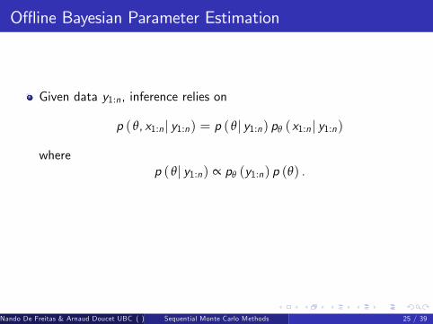
O ine Bayesian Parameter Estimation
Given data y1:n, inference relies on
p ( θ, x1:n j y1:n) = p ( θj y1:n) pθ (x1:n j y1:n)
wherep ( θj y1:n) ∝ pθ (y1:n) p (θ) .
For a given θ, SMC can estimate both pθ (x1:n j y1:n) and pθ (y1:n).
Is it possible to use SMC within MCMC to sample fromp ( θ, x1:n j y1:n)?
Nando De Freitas & Arnaud Doucet UBC ( ) Sequential Monte Carlo Methods 25 / 39

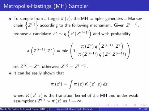
Metropolis-Hastings (MH) Sampler
To sample from a target π (z), the MH sampler generates a Markov
chainnZ (i )
oaccording to the following mechanism. Given Z (i�1),
propose a candidate Z � � q�z�jZ (i�1)
�and with probability
α�Z (i�1),Z �
�= min
0@1, π (Z �) q�Z (i�1)
���Z ��π�Z (i�1)
�q�Z �jZ (i�1)
�1A
set Z (i ) = Z �, otherwise Z (i ) = Z (i�1).
It can be easily shown that
π�z 0�=Z
π (z)K�z 0�� z� dz
where K (z 0j z) is the transition kernel of the MH and under weakassumptions Z (i ) � π (z) as i ! ∞.
Nando De Freitas & Arnaud Doucet UBC ( ) Sequential Monte Carlo Methods 26 / 39

Marginal Metropolis-Hastings Sampler
Consider the following so-called marginal MH algorithm which target
p ( θ, x1:n j y1:n) = p ( θj y1:n) pθ (x1:n j y1:n)
using the proposal
q ( (x�1:n, θ�)j (x1:n, θ)) = q ( θ�j θ) pθ� (x
�1:n j y1:n) .
The MH acceptance probability is
min�1,p ( θ�, x�1:n j y1:n)
p ( θ, x1:n j y1:n)
q ( (x1:n, θ)j (x�1:n, θ�))
q ( (x�1:n, θ�)j (x1:n, θ))
�= min
�1,pθ� (y1:n) p (θ�)pθ (y1:n) p (θ)
q ( θj θ�)q ( θ�j θ)
�Problem: We do not know pθ (y1:n) analytically and cannot samplefrom pθ (x1:n j y1:n) so this algorithm cannot be implemented.�Idea�: Use SMC approximations of pθ (x1:n j y1:n) and pθ (y1:n).
Nando De Freitas & Arnaud Doucet UBC ( ) Sequential Monte Carlo Methods 27 / 39

Marginal Metropolis-Hastings Sampler
Consider the following so-called marginal MH algorithm which target
p ( θ, x1:n j y1:n) = p ( θj y1:n) pθ (x1:n j y1:n)
using the proposal
q ( (x�1:n, θ�)j (x1:n, θ)) = q ( θ�j θ) pθ� (x
�1:n j y1:n) .
The MH acceptance probability is
min�1,p ( θ�, x�1:n j y1:n)
p ( θ, x1:n j y1:n)
q ( (x1:n, θ)j (x�1:n, θ�))
q ( (x�1:n, θ�)j (x1:n, θ))
�= min
�1,pθ� (y1:n) p (θ�)pθ (y1:n) p (θ)
q ( θj θ�)q ( θ�j θ)
�
Problem: We do not know pθ (y1:n) analytically and cannot samplefrom pθ (x1:n j y1:n) so this algorithm cannot be implemented.�Idea�: Use SMC approximations of pθ (x1:n j y1:n) and pθ (y1:n).
Nando De Freitas & Arnaud Doucet UBC ( ) Sequential Monte Carlo Methods 27 / 39

Marginal Metropolis-Hastings Sampler
Consider the following so-called marginal MH algorithm which target
p ( θ, x1:n j y1:n) = p ( θj y1:n) pθ (x1:n j y1:n)
using the proposal
q ( (x�1:n, θ�)j (x1:n, θ)) = q ( θ�j θ) pθ� (x
�1:n j y1:n) .
The MH acceptance probability is
min�1,p ( θ�, x�1:n j y1:n)
p ( θ, x1:n j y1:n)
q ( (x1:n, θ)j (x�1:n, θ�))
q ( (x�1:n, θ�)j (x1:n, θ))
�= min
�1,pθ� (y1:n) p (θ�)pθ (y1:n) p (θ)
q ( θj θ�)q ( θ�j θ)
�Problem: We do not know pθ (y1:n) analytically and cannot samplefrom pθ (x1:n j y1:n) so this algorithm cannot be implemented.
�Idea�: Use SMC approximations of pθ (x1:n j y1:n) and pθ (y1:n).
Nando De Freitas & Arnaud Doucet UBC ( ) Sequential Monte Carlo Methods 27 / 39

Marginal Metropolis-Hastings Sampler
Consider the following so-called marginal MH algorithm which target
p ( θ, x1:n j y1:n) = p ( θj y1:n) pθ (x1:n j y1:n)
using the proposal
q ( (x�1:n, θ�)j (x1:n, θ)) = q ( θ�j θ) pθ� (x
�1:n j y1:n) .
The MH acceptance probability is
min�1,p ( θ�, x�1:n j y1:n)
p ( θ, x1:n j y1:n)
q ( (x1:n, θ)j (x�1:n, θ�))
q ( (x�1:n, θ�)j (x1:n, θ))
�= min
�1,pθ� (y1:n) p (θ�)pθ (y1:n) p (θ)
q ( θj θ�)q ( θ�j θ)
�Problem: We do not know pθ (y1:n) analytically and cannot samplefrom pθ (x1:n j y1:n) so this algorithm cannot be implemented.�Idea�: Use SMC approximations of pθ (x1:n j y1:n) and pθ (y1:n).
Nando De Freitas & Arnaud Doucet UBC ( ) Sequential Monte Carlo Methods 27 / 39

Particle Marginal MH Sampler
At iteration i , given fθ (i � 1) ,X1:n (i � 1) ,bpθ(i�1) (y1:n)g thensample θ� � q ( θj θ (i � 1)), run an SMC algorithm to obtainbpθ� (x1:n j y1:n) and bpθ� (y1:n).
Sample X �1:n � bpθ� (x1:n j y1:n) .
With probability
min
1,
bpθ� (y1:n) p (θ�)bpθ(i�1) (y1:n) p (θ (i � 1))q ( θ (i � 1)j θ�)q ( θ�j θ (i � 1))
!
set fθ (i) ,X1:n (i) ,bpθ(i ) (y1:n)g = fθ�,X �1:n,bpθ� (y1:n)g otherwise setfθ (i) ,X1:n (i) ,bpθ(i ) (y1:n)g = fθ (i � 1) ,X1:n (i � 1) ,bpθ(i�1) (y1:n)g.
Nando De Freitas & Arnaud Doucet UBC ( ) Sequential Monte Carlo Methods 28 / 39

Validity of the Particle Marginal MH Sampler
This algorithm (without sampling X1:n) was proposed as anapproximate MCMC algorithm to sample from p ( θj y1:n) in(Fernandez-Villaverde & Rubio-Ramirez, 2007).
Whatever being N � 1, this algorithm admits exactly p ( θ, x1:n j y1:n)as invariant distribution (Andrieu, D. & Holenstein, 2010). A particleversion of the Gibbs sampler also exists.
The higher N, the better the performance of the algorithm: N scalesroughly linearly with n.
Particularly useful in scenarios where Xn moderate dimensional & θhigh dimensional. Admits the plug and play property (Ionides et al.,2006).
Nando De Freitas & Arnaud Doucet UBC ( ) Sequential Monte Carlo Methods 29 / 39

Inference for Stochastic Kinetic Models
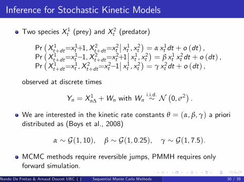
Two species X 1t (prey) and X2t (predator)
Pr�X 1t+dt=x
1t+1,X
2t+dt=x
2t
�� x1t , x2t � = α x1t dt + o (dt) ,Pr�X 1t+dt=x
1t�1,X 2t+dt=x2t+1
�� x1t , x2t � = β x1t x2t dt + o (dt) ,
Pr�X 1t+dt=x
1t ,X
2t+dt=x
2t�1
�� x1t , x2t � = γ x2t dt + o (dt) ,
observed at discrete times
Yn = X 1n∆ +Wn with Wni.i.d.� N
�0, σ2
�.
We are interested in the kinetic rate constants θ = (α, β,γ) a prioridistributed as (Boys et al., 2008)
α � G(1, 10), β � G(1, 0.25), γ � G(1, 7.5).
MCMC methods require reversible jumps, PMMH requires onlyforward simulation.
Nando De Freitas & Arnaud Doucet UBC ( ) Sequential Monte Carlo Methods 30 / 39

Inference for Stochastic Kinetic Models
Two species X 1t (prey) and X2t (predator)
Pr�X 1t+dt=x
1t+1,X
2t+dt=x
2t
�� x1t , x2t � = α x1t dt + o (dt) ,Pr�X 1t+dt=x
1t�1,X 2t+dt=x2t+1
�� x1t , x2t � = β x1t x2t dt + o (dt) ,
Pr�X 1t+dt=x
1t ,X
2t+dt=x
2t�1
�� x1t , x2t � = γ x2t dt + o (dt) ,
observed at discrete times
Yn = X 1n∆ +Wn with Wni.i.d.� N
�0, σ2
�.
We are interested in the kinetic rate constants θ = (α, β,γ) a prioridistributed as (Boys et al., 2008)
α � G(1, 10), β � G(1, 0.25), γ � G(1, 7.5).
MCMC methods require reversible jumps, PMMH requires onlyforward simulation.
Nando De Freitas & Arnaud Doucet UBC ( ) Sequential Monte Carlo Methods 30 / 39

Experimental Results
20
0
20
40
60
80
100
120
140
0 1 2 3 4 5 6 7 8 9 10
p r eyp r edator
Simulated data
1. 5 2 2. 5 3 3. 5 4 4. 51 . 5 2 2. 5 3 3. 5 4 4. 5 0. 06 0. 12 0. 180. 06 0. 12 0. 18 1 2 3 4 5 6 7 81 2 3 4 5 6 7 8
α
β
γ
Posterior distributions
Nando De Freitas & Arnaud Doucet UBC ( ) Sequential Monte Carlo Methods 31 / 39

SMC Fixed-Lag Smoothing Approximation
Direct SMC approximations of p (x1:n j y1:n) and its marginalsp (xk j y1:n) gets poorer as n %.
The �xed-lag smoothing approximation (Kitagawa & Sato, 2001)relies on
p (x1:k j y1:n) � p (x1:k j y1:k+∆) for ∆ large enough.
Algorithmically: stop resamplingnX (i )k
obeyond time k + ∆.
Computational cost is O (Nn) but non-vanishing bias as N ! ∞(Olsson & al., 2006).
Picking ∆ is di¢ cult. ∆ too small results in p (x1:k j y1:k+∆) being apoor approximation of p (x1:k j y1:n). ∆ too large improves theapproximation but particle degeneracy creeps in.
Nando De Freitas & Arnaud Doucet UBC ( ) Sequential Monte Carlo Methods 32 / 39
SMC Fixed-Lag Smoothing Approximation
Direct SMC approximations of p (x1:n j y1:n) and its marginalsp (xk j y1:n) gets poorer as n %.The �xed-lag smoothing approximation (Kitagawa & Sato, 2001)relies on
p (x1:k j y1:n) � p (x1:k j y1:k+∆) for ∆ large enough.
Algorithmically: stop resamplingnX (i )k
obeyond time k + ∆.
Computational cost is O (Nn) but non-vanishing bias as N ! ∞(Olsson & al., 2006).
Picking ∆ is di¢ cult. ∆ too small results in p (x1:k j y1:k+∆) being apoor approximation of p (x1:k j y1:n). ∆ too large improves theapproximation but particle degeneracy creeps in.
Nando De Freitas & Arnaud Doucet UBC ( ) Sequential Monte Carlo Methods 32 / 39

SMC Forward Filtering Backward Smoothing
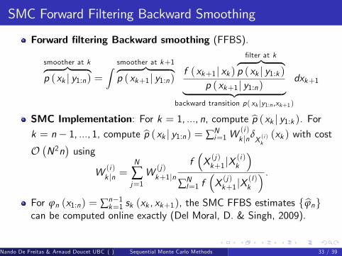
Forward �ltering Backward smoothing (FFBS).
smoother at kz }| {p (xk j y1:n) =
Z smoother at k+1z }| {p (xk+1j y1:n)
f (xk+1j xk )�lter at kz }| {
p (xk j y1:k )
p (xk+1j y1:n)| {z }backward transition p( xk jy1:n ,xk+1)
dxk+1
SMC Implementation: For k = 1, ..., n, compute bp (xk j y1:k ). For
k = n� 1, ..., 1, compute bp (xk j y1:n) = ∑Ni=1W
(i )k jnδ
X (i )k(xk ) with cost
O�N2n
�using
W (i )k jn =
N
∑j=1W (j)k+1jn
f�X (j)k+1jX
(i )k
�∑Nl=1 f
�X (j)k+1jX
(l)k
� .For ϕn (x1:n) = ∑n�1
k=1 sk (xk , xk+1), the SMC FFBS estimates fbϕngcan be computed online exactly (Del Moral, D. & Singh, 2009).Sampling from bp (x1:n j y1:n) costs O(Nn) (Godsill, D. & West, 2004)but O(n) through rejection sampling (Douc et al., 2009).
Nando De Freitas & Arnaud Doucet UBC ( ) Sequential Monte Carlo Methods 33 / 39

SMC Forward Filtering Backward Smoothing
Forward �ltering Backward smoothing (FFBS).
smoother at kz }| {p (xk j y1:n) =
Z smoother at k+1z }| {p (xk+1j y1:n)
f (xk+1j xk )�lter at kz }| {
p (xk j y1:k )
p (xk+1j y1:n)| {z }backward transition p( xk jy1:n ,xk+1)
dxk+1
SMC Implementation: For k = 1, ..., n, compute bp (xk j y1:k ). For
k = n� 1, ..., 1, compute bp (xk j y1:n) = ∑Ni=1W
(i )k jnδ
X (i )k(xk ) with cost
O�N2n
�using
W (i )k jn =
N
∑j=1W (j)k+1jn
f�X (j)k+1jX
(i )k
�∑Nl=1 f
�X (j)k+1jX
(l)k
� .
For ϕn (x1:n) = ∑n�1k=1 sk (xk , xk+1), the SMC FFBS estimates fbϕng
can be computed online exactly (Del Moral, D. & Singh, 2009).Sampling from bp (x1:n j y1:n) costs O(Nn) (Godsill, D. & West, 2004)but O(n) through rejection sampling (Douc et al., 2009).
Nando De Freitas & Arnaud Doucet UBC ( ) Sequential Monte Carlo Methods 33 / 39
SMC Forward Filtering Backward Smoothing
Forward �ltering Backward smoothing (FFBS).
smoother at kz }| {p (xk j y1:n) =
Z smoother at k+1z }| {p (xk+1j y1:n)
f (xk+1j xk )�lter at kz }| {
p (xk j y1:k )
p (xk+1j y1:n)| {z }backward transition p( xk jy1:n ,xk+1)
dxk+1
SMC Implementation: For k = 1, ..., n, compute bp (xk j y1:k ). For
k = n� 1, ..., 1, compute bp (xk j y1:n) = ∑Ni=1W
(i )k jnδ
X (i )k(xk ) with cost
O�N2n
�using
W (i )k jn =
N
∑j=1W (j)k+1jn
f�X (j)k+1jX
(i )k
�∑Nl=1 f
�X (j)k+1jX
(l)k
� .For ϕn (x1:n) = ∑n�1
k=1 sk (xk , xk+1), the SMC FFBS estimates fbϕngcan be computed online exactly (Del Moral, D. & Singh, 2009).
Sampling from bp (x1:n j y1:n) costs O(Nn) (Godsill, D. & West, 2004)but O(n) through rejection sampling (Douc et al., 2009).
Nando De Freitas & Arnaud Doucet UBC ( ) Sequential Monte Carlo Methods 33 / 39

SMC Forward Filtering Backward Smoothing
Forward �ltering Backward smoothing (FFBS).
smoother at kz }| {p (xk j y1:n) =
Z smoother at k+1z }| {p (xk+1j y1:n)
f (xk+1j xk )�lter at kz }| {
p (xk j y1:k )
p (xk+1j y1:n)| {z }backward transition p( xk jy1:n ,xk+1)
dxk+1
SMC Implementation: For k = 1, ..., n, compute bp (xk j y1:k ). For
k = n� 1, ..., 1, compute bp (xk j y1:n) = ∑Ni=1W
(i )k jnδ
X (i )k(xk ) with cost
O�N2n
�using
W (i )k jn =
N
∑j=1W (j)k+1jn
f�X (j)k+1jX
(i )k
�∑Nl=1 f
�X (j)k+1jX
(l)k
� .For ϕn (x1:n) = ∑n�1
k=1 sk (xk , xk+1), the SMC FFBS estimates fbϕngcan be computed online exactly (Del Moral, D. & Singh, 2009).Sampling from bp (x1:n j y1:n) costs O(Nn) (Godsill, D. & West, 2004)but O(n) through rejection sampling (Douc et al., 2009).
Nando De Freitas & Arnaud Doucet UBC ( ) Sequential Monte Carlo Methods 33 / 39
SMC Generalized Two-Filter Smoothing
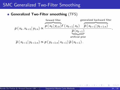
Generalized Two-Filter smoothing (TFS)
p (xk , xk+1j y1:n) ∝
forward �lterz }| {p (xk j y1:k )f (xk+1j xk )
generalized backward �lterz }| {p (xk+1j yk+1:n)
p (xk+1)| {z }arti�cial prior
,
p (xk+1j yk+1:n) ∝ p (yk+1:n j xk+1) p (xk+1) .
SMC Implementation: For k = 1, ..., n, compute bp (xk j y1:k ). Fork = n, ..., 1, compute bp (xk+1j yk+1:n). Combine the forward andbackward �lters to obtain
bp (xk , xk+1j y1:n) ∝ bp (xk j y1:k )f (xk+1j xk )p (xk+1)
bp (xk+1j yk+1:n)
Cost O�N2n
�but O (Nn) through rejection sampling (Briers, D. &
Maskell, 2008) and importance sampling (Fearnhead, Wyncoll &Tawn, 2008; Briers, D. & Singh, 2005).
Nando De Freitas & Arnaud Doucet UBC ( ) Sequential Monte Carlo Methods 34 / 39

SMC Generalized Two-Filter Smoothing
Generalized Two-Filter smoothing (TFS)
p (xk , xk+1j y1:n) ∝
forward �lterz }| {p (xk j y1:k )f (xk+1j xk )
generalized backward �lterz }| {p (xk+1j yk+1:n)
p (xk+1)| {z }arti�cial prior
,
p (xk+1j yk+1:n) ∝ p (yk+1:n j xk+1) p (xk+1) .SMC Implementation: For k = 1, ..., n, compute bp (xk j y1:k ). Fork = n, ..., 1, compute bp (xk+1j yk+1:n). Combine the forward andbackward �lters to obtain
bp (xk , xk+1j y1:n) ∝ bp (xk j y1:k )f (xk+1j xk )p (xk+1)
bp (xk+1j yk+1:n)
Cost O�N2n
�but O (Nn) through rejection sampling (Briers, D. &
Maskell, 2008) and importance sampling (Fearnhead, Wyncoll &Tawn, 2008; Briers, D. & Singh, 2005).
Nando De Freitas & Arnaud Doucet UBC ( ) Sequential Monte Carlo Methods 34 / 39

Convergence Results
Exponentially stability assumption. For any x1, x 01
12
Z ��p (xn j y2:n,X1 = x1)� p�xn j y2:n,X1 = x 01
��� dxn � αn for jαj < 1.
Additive functionals. If ϕn (x1:n) = ∑nk=1 ϕ (xk ) , we have for the
standard path-based SMC estimate (Poyiadjis, D. & Singh, 2009)
limN!∞
pN (bϕn � ϕn)) N
�0, σ2n
�where An2 � σ2n � An2.
For the FFBS and TFS estimates (Douc et al., 2009; Del Moral, D. &Singh, 2009), we have
limN!∞
pN (bϕn � ϕn)) N
�0, σ2n
�where σ2n � Cn
Tradeo¤ between computational and statistical e¢ ciency.
Nando De Freitas & Arnaud Doucet UBC ( ) Sequential Monte Carlo Methods 35 / 39

Experimental Results
Consider a linear Gaussian model
X1 � N�0,
σ2
1� φ2
�and Xk = φXk�1 + σVVk , Vk
i.i.d.� N (0, 1)
Yk = cXk + σWWk , Wki.i.d.� N (0, 1) .
We simulate 10,000 observations forθ = (φ, σV , c , σW ) = (0.8, 0.5, 1.0, 1.0).
We compute the score vector using Fisher�s identity
r log pθ (y1:n) =Zr log pθ (x1:n, y1:n) pθ (x1:n j y1:n) dx1:n
at the true value of θ and compare to its true value.
Nando De Freitas & Arnaud Doucet UBC ( ) Sequential Monte Carlo Methods 36 / 39

Empirical Variance for Standard vs FFBS Approximations
0 2 5 0 0 5 0 0 0 7 5 0 0 1 0 0 0 00
2
4
6
x 1 04
V arianc e of s core es t im at e w . r. t .σv
Var
ianc
e
0 2 5 0 0 5 0 0 0 7 5 0 0 1 0 0 0 00
2 0 0 0
4 0 0 0
6 0 0 0
8 0 0 0
1 0 0 0 0
V arianc e of s core es t im at e w . r. t .φ
0 2 5 0 0 5 0 0 0 7 5 0 0 1 0 0 0 00
1 0 0 0
2 0 0 0
3 0 0 0
4 0 0 0
V arianc e of s core es t im at e w . r. t .σw
T im e s te p s
Var
ianc
e
0 2 5 0 0 5 0 0 0 7 5 0 0 1 0 0 0 00
1 0 0 0
2 0 0 0
3 0 0 0
4 0 0 0
5 0 0 0
V arianc e of s core es t im at e w . r. t . c
T im e s te p s
0 2 5 0 0 5 0 0 0 7 5 0 0 1 0 0 0 00
2 0
4 0
6 0
8 0
1 0 0
1 2 0
V arianc e of s core es t im at e w . r. t .σv
Var
ianc
e
0 2 5 0 0 5 0 0 0 7 5 0 0 1 0 0 0 00
2 0
4 0
6 0
V arianc e of s c ore es t im at e w . r . t .φ
0 2 5 0 0 5 0 0 0 7 5 0 0 1 0 0 0 00
5
1 0
1 5
2 0
V arianc e of s core es t im at e w . r. t .σw
T im e s te p s
Var
ianc
e
0 2 5 0 0 5 0 0 0 7 5 0 0 1 0 0 0 00
1 0
2 0
3 0
4 0
V arianc e of s core es t im at e w . r. t . c
T im e s te p s
Standard path-based (left) vs FFBS (right); the vertical scale is di¤erent
Nando De Freitas & Arnaud Doucet UBC ( ) Sequential Monte Carlo Methods 37 / 39

Parameter Estimation using Gradient Ascent/EM
Gradient ascent: To maximise pθ(y1:n) w.r.t θ, use at iteration k + 1
θk+1 = θk + r log pθ (y1:n)jθ=θk
where r log pθ (y1:n)jθ=θkis computed using Fisher�s identity or IPA
(Coquelin, Deguest & Munos, 2009) and any SMC smoothingalgorithm.
EM algorithm: To maximise pθ(y1:n) w.r.t θ, the EM uses at iterationk + 1
θk+1 = argmax Q(θk , θ).
where
Q(θk , θ) =Zlog pθ(x1:n, y1:n) pθk (x1:n jy1:n)dx1:n
can be computed using any SMC smoothing algorithm.
Nando De Freitas & Arnaud Doucet UBC ( ) Sequential Monte Carlo Methods 38 / 39

Online Parameter Estimation using Gradient Ascent/EM
In the online implementation (Le Gland & Mevel, 1997), update theparameter at time n+ 1 using
θn+1 = θn + γn+1r log pθ1:n (yn jy1:n�1)
where ∑n γn = ∞, ∑n γ2n < ∞ and
r log pθ1:n (yn jy1:n�1) = r log pθ1:n (y1:n)�r log pθ1:n�1(y1:n�1).
An estimate of r log pθ1:n (yn jy1:n�1) with a time-uniform boundedvariance can be computed using online SMC FFBS estimate (DelMoral, D. & Singh, 2009).A numerically stable SMC implementation of online EM (e.g. Cappé,2009; Elliott, Ford & Moore, 2002) can also be implemented usingonline SMC FFBS estimate.These non-Bayesian procedures do not su¤er from the degeneracyproblem but require long data sets for convergence.
Nando De Freitas & Arnaud Doucet UBC ( ) Sequential Monte Carlo Methods 39 / 39

Online Parameter Estimation using Gradient Ascent/EM
In the online implementation (Le Gland & Mevel, 1997), update theparameter at time n+ 1 using
θn+1 = θn + γn+1r log pθ1:n (yn jy1:n�1)
where ∑n γn = ∞, ∑n γ2n < ∞ and
r log pθ1:n (yn jy1:n�1) = r log pθ1:n (y1:n)�r log pθ1:n�1(y1:n�1).
An estimate of r log pθ1:n (yn jy1:n�1) with a time-uniform boundedvariance can be computed using online SMC FFBS estimate (DelMoral, D. & Singh, 2009).
A numerically stable SMC implementation of online EM (e.g. Cappé,2009; Elliott, Ford & Moore, 2002) can also be implemented usingonline SMC FFBS estimate.These non-Bayesian procedures do not su¤er from the degeneracyproblem but require long data sets for convergence.
Nando De Freitas & Arnaud Doucet UBC ( ) Sequential Monte Carlo Methods 39 / 39

Online Parameter Estimation using Gradient Ascent/EM
In the online implementation (Le Gland & Mevel, 1997), update theparameter at time n+ 1 using
θn+1 = θn + γn+1r log pθ1:n (yn jy1:n�1)
where ∑n γn = ∞, ∑n γ2n < ∞ and
r log pθ1:n (yn jy1:n�1) = r log pθ1:n (y1:n)�r log pθ1:n�1(y1:n�1).
An estimate of r log pθ1:n (yn jy1:n�1) with a time-uniform boundedvariance can be computed using online SMC FFBS estimate (DelMoral, D. & Singh, 2009).A numerically stable SMC implementation of online EM (e.g. Cappé,2009; Elliott, Ford & Moore, 2002) can also be implemented usingonline SMC FFBS estimate.
These non-Bayesian procedures do not su¤er from the degeneracyproblem but require long data sets for convergence.
Nando De Freitas & Arnaud Doucet UBC ( ) Sequential Monte Carlo Methods 39 / 39

Online Parameter Estimation using Gradient Ascent/EM
In the online implementation (Le Gland & Mevel, 1997), update theparameter at time n+ 1 using
θn+1 = θn + γn+1r log pθ1:n (yn jy1:n�1)
where ∑n γn = ∞, ∑n γ2n < ∞ and
r log pθ1:n (yn jy1:n�1) = r log pθ1:n (y1:n)�r log pθ1:n�1(y1:n�1).
An estimate of r log pθ1:n (yn jy1:n�1) with a time-uniform boundedvariance can be computed using online SMC FFBS estimate (DelMoral, D. & Singh, 2009).A numerically stable SMC implementation of online EM (e.g. Cappé,2009; Elliott, Ford & Moore, 2002) can also be implemented usingonline SMC FFBS estimate.These non-Bayesian procedures do not su¤er from the degeneracyproblem but require long data sets for convergence.
Nando De Freitas & Arnaud Doucet UBC ( ) Sequential Monte Carlo Methods 39 / 39

Tutorial overview• Introduction Nando – 10min
• Part I Arnaud – 50min
– Monte Carlo
– Sequential Monte Carlo
– Theoretical convergence
– Improved particle filters
– Online Bayesian parameter estimation
– Particle MCMC
– Smoothing
– Gradient based online parameter estimation
• Break 15min
• Part II NdF – 45 min
– Beyond state space models
– Eigenvalue problems
– Diffusion, protein folding & stochastic control
– Time-varying Pitman-Yor Processes
– SMC for static distributions
– Boltzmann distributions & ABC

y1
Sequential Monte Carlo (recap)
X0 X1X3X2
Y1 Y2 Y3
P(X 0) P(X2jX1)P(Y2jX2)P(X1jX0)P(Y1jX1) P(X3jX 2)P(Y3jX3) / P(X0:3jY1:3)

Sequences of distributions
² SMC methods can be used to sample approximately from any sequence of
growing dist ribut ions f ¼n gn ¸ 1
¼n (x1:n ) =f n (x1:n )
Zn
where
{ f n : X n ! R+ is known point -wise.
{ Zn =R
f n (x1:n )dx1:n
² We int roduce a proposal dist ribut ion qn (x1:n ) to approzimate Zn :
Zn =
Zf n (x1:n )
qn (x1:n )qn (x1:n )dx1:n =
Z
Wn (x1:n ) qn (x1:n )dx1:n

Importance weights² Let us const ruct the proposal sequent ially: Int roduce qn ( xn j x1:n ¡ 1) to
sample component X n given X 1:n ¡ 1 = x1:n ¡ 1:
² Then the importance weight becomes:
Wn = Wn ¡ 1
f n (x1:n )
f n ¡ 1 (x1:n ¡ 1)qn ( xn j x1:n ¡ 1)

SMC algorithm1. Initialize at time n = 1
2. At time n ¸ 2
² Sample X( i )
n » qn
³xn j X
( i )1:n ¡ 1
´and augment X
( i )
1:n =³
X( i )1:n ¡ 1; X
( i )
n
´
² Resample X( i )1:n » e¼n (x1:n ) to obtain b¼n (x1:n ) = 1
N
P Ni = 1 ±
X( i )1 :n
(x1:n ).
² Compute the sequential weight
W ( i )n /
f n
³X
( i )
1:n
´
f n ¡ 1
³X
( i )
1:n ¡ 1
´qn
³X
( i )
n
¯¯¯X
( i )
1:n ¡ 1
´ :
Then the target approximation is:
e¼n (x1:n ) =
NX
i = 1
W ( i )n ±
X( i )
1 :n
(x1:n )

Example 1: Bayesian filteringf n (x1:n ) = p(x1:n ; y1:n ); ¼n (x1:n ) = p( x1:n j y1:n ) ; Zn = p(y1:n );
qn ( xn j x1:n ¡ 1) = f ( xn j x1:n ¡ 1):

Example 2: Eigen-particles
Computing eigen-pairs of exponentially large matrices and operators is
an important problem in science. I will give two motivating examples:
i. Diffusion equation & Schrodinger’s equation in quantum physics
ii. Transfer matrices for estimating the partition function of
Boltzmann machines
Both problems are of enormous importance in physics and learning.

Quantum Monte Carlo
We can map this mult ivariable di®erent ial equat ion to an eigenvalue problem:
Z
Ã(r )K (sjr )dr = ¸ Ã(s)
In the discrete case, this is the largest eigenpair of the M £ M matrix A:
Ax = ¸ x ´
MX
i = 1
x(r )a(r; s) = ¸ x(s) ; s = 1; 2; : : : ; M
where a(r; s) is the ent ry of A at row r and column s.
[JB Anderson, 1975, I Kosztin et al, 1997]

Transfer matrices of Boltzmann Machines
Z =X
f ¹ g
nY
j = 1
exp
Ã
º
mX
i = 1
¹ i ;j ¹ i + 1;j + º
mX
i = 1
¹ i ;j ¹ i ;j + 1
!
=X
f ¾1 ;:::;¾n g
nY
j = 1
A(¾j ; ¾j + 1) =
2m
X
k= 1
¸ nk ¾j = (¹ 1;j ; : : : ; ¹ m ;j )
[see e.g. Onsager, Nimalan Mahendran]
¹ i ;j¹ i ;j 2 f ¡ 1; 1g

Power methodLet A have M linearly independent eigenvectors, then any vector v may be
represented as a linear combinat ion of the eigenvectors of A: v =P
i ci x i ,
where c is a constant . Consequent ly, for su± cient ly large n,
An v ¼ c1¸ n1 x1

Particle power methodSuccesive matrix-vector mult iplicat ion maps to Kernel-funct ion mult iplicat ion
(a path integral) in the cont inuous case:
Z
¢¢¢
Z
v(x1)
nY
k= 2
K (xk jxk ¡ 1)dx1:n ¡ 1 ¼ c1¸ n1 Ã(xn )
The part icle method is obtained by de ning
f (x1:n ) = v(x1)
nY
k= 2
K (x k jx k ¡ 1)
Consequent ly c¸ n1 ¡ ! Zn and Ã(xn ) ¡ ! ¼(xn ). The largest eigenvalue ¸ 1 of
K is given by the rat io of successive part it ion funct ions:
¸ 1 =Zn
Zn ¡ 1The importance weights are
Wn = Wn ¡ 1
v(x1)Q n
k= 2 K (xk jxk ¡ 1)
Q(xn jx1:n )v(x1)Q n ¡ 1
k= 2 K (xk jxk ¡ 1)= Wn ¡ 1
K (xn jxn ¡ 1)
Q(xn jx1:n )

Example 3: Particle diffusion
² A part icle f X n gn ¸ 1 evolves in a random medium
X 1 » ¹ (¢) , X n + 1j X n = x » p( ¢j x) :
² At t imen, theprobability of it being killed is1¡ g(X n ) with 0 · g(x) · 1.
² One wants to approximate Pr (T > n).
?

Example 3: Particle diffusion² Again, we obtain our familiar path integral:
Pr (T > n) = E¹ [Probability of not being killed at n given X 1:n ]
=
Z
¢¢¢
Z
¹ (x1)
nY
k = 2
p( xk j xk ¡ 1)
nY
k = 1
g(xk )
| {z }Probabi l i t y t o surv ive at n
dx1:n
² Consider
f n (x1:n ) = ¹ (x1)
nY
k = 2
p( xk j xk ¡ 1)
nY
k= 1
g(xk )
¼n (x1:n ) =f n (x1:n )
Zn
where Zn = Pr (T > n)
² SMC is then used to compute Zn , the probability of not being killed at
t ime n, and to approximate the dist ribut ion of the paths having survived
at t ime n.
[Del Moral & AD, 2004]

Example 4: SAWs
SAWs on lattices are often used to study polymers and protein folding.
[See e.g. Peter Grassberger (PERM) & Alena Shmygelska; Rosenbluth Method]
Goal: Compute the volume Zn of a self-avoiding random walk, with uniform
dist ribut ion on a lat t ice:
¼n (x1:n ) = Zn¡ 11D n
(x1:n )
where
Dn = f x1:n 2 En such that xk » xk+ 1 and xk 6= x i for k 6= ig;
Zn = cardinality of Dn :

Example 5: Stochastic control
[AD & Vladislav Tadic, 2005]
² Consider a Fredholm equat ion of the 2nd kind (e.g. Bellman backup):
v(x0) = r (x0) +
Z
K (x0; x1)v(x1)dx1
² This expression can be easily t ransformed into a path integral (Von Neu-
mann series representat ion):
v(x0) = r (x0) +
1X
n = 1
Z
r (xn )
nY
k= 1
K (xk ¡ 1; xk )dx1:n
² The SMC sampler again follows by choosing
f 0 (x0) = r (x0)
f n (x0:n ) = r (xn )
nY
k = 1
K (xk ¡ 1; xk )
² In this case we have a t rans-dimensional dist ribut ion, so we do a lit t le bit
more work when implement ing the method.

Particle smoothing can be used in the E
step of the EM algorithm for MDPs
x1
a1
x2
a2
x3
a3
r
Marginal likelihood
Likelihood PriorMDP posterior
[See e.g. Matt Hoffman et al, 2007]

Example 6: Dynamic Dirichlet processes
[Francois Caron, Manuel Davy & AD, 2007]

SMC for static models
X 2
X 3
X 1
X 4 X 5
X 2
X 3
X 1
X 4 X 5
X 2
X 3
X 1
X 4 X 5
² Let f ¼n gn ¸ 1 be a sequence of probability dist ribut ions de ned on X such
that each ¼n (x) is known up to a normalizing constant , i.e.
¼n (x) = Zn¡ 1
| {z }unknown
f n (x)| {z }known
² We want to sample approximately from ¼n (x) and compute Zn sequen-
t ially.
² This di®ers from the standard SMC, where ¼n (x1:n ) is de ned on X n .
¼n (x) = Z ¡ 1eP
i
Pj x i w i j x j
X 2
X 3
X 1
X 4 X 5 …
¼3(x)¼2(x)¼1(x)
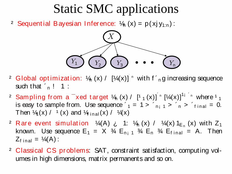
Static SMC applications² Sequent ial Bayesian Inference: ¼n (x) = p( xj y1:n ) :
X
Y1 Y2 Yn
² Global opt imizat ion: ¼n (x) / [¼(x)]´ n with f ´ n g increasing sequence
such that ´ n ! 1 :
Y3…
² Sampling fr om a ¯xed t ar get ¼n (x) / [¹ 1 (x)]´ n [¼(x)]
1¡ ´ n where ¹ 1
is easy to sample from. Use sequence ´ 1 = 1 > ´ n ¡ 1 > ´ n > ´ f i n al = 0.
Then ¼1(x) / ¹ (x) and ¼f i n al (x) / ¼(x)
² Rare event simulat ion ¼(A) ¿ 1: ¼n (x) / ¼(x) 1E n(x) with Z1
known. Use sequence E1 = X ¾ En ¡ 1 ¾ En ¾ Ef i nal = A. Then
Zf i nal = ¼(A) :
² Classical CS problems: SAT, constraint sat isfact ion, computing vol-
umes in high dimensions, matrix permanents and so on.

Static SMC derivation² Const ruct an art i¯cial dist ribut ion that is the product of the target dis-
t ribut ion that we want to sample from and a backward kernel L :
e¼n (x1:n ) = Zn¡ 1f n (x1:n ), where f n (x1:n ) = f n (xn )
| {z }t arget
n ¡ 1Y
k= 1
L k ( xk j xk+ 1)
| {z }ar t i¯cial backward t ransi t ions
such that ¼n (xn ) =R
e¼n (x1:n ) dx1:n .
[Pierre Del Moral, AD, Ajay Jasra, 2006]
² The importance weights become:
Wn =f n (x1:n )
K n (x1:n )= Wn ¡ 1
K n ¡ 1(x1:n ¡ 1)
f n ¡ 1(x1:n ¡ 1)
f n (x1:n )
K n (x1:n )
= Wn ¡ 1
f n (xn )L n ¡ 1(xn ¡ 1jxn )
f n ¡ 1 (xn ¡ 1)K n (xn jxn ¡ 1)
² For the proposal K (:), we can use any MCMC kernel.
² We only care about ¼n (xn ) = Z ¡ 1f n (xn ) so no degeneracy problem.

Static SMC algorithm
1. Init ialize at time n = 1
2. At time n ¸ 2
(a) SampleX( i )
n » K n
³xn j X
( i )n ¡ 1
´and augment X
( i )
n ¡ 1:n =³
X( i )n ¡ 1; X
( i )
n
´
(b) Compute the importance weights
W ( i )n = W
( i )n ¡ 1
f n
³X
( i )
n
´L n ¡ 1
³X
( i )
n ¡ 1
¯¯¯X
( i )
n
´
f n ¡ 1
³X
( i )
n ¡ 1
´K n
³X
( i )
n
¯¯¯X
( i )
n ¡ 1
´ :
Then the weighted approximation is
e¼n (xn ) =
NX
i = 1
W ( i )n ±
X( i )
n
(xn )
(c) Resample X( i )n » e¼n (xn ) to obtain b¼n (xn ) = 1
N
P Ni = 1 ±
X( i )n
(xn ).

Static SMC: Choice of L
² A default (easiest ) choice consists of using a ¼n -invariant MCMC kernel
K n and the corresponding reversed kernel L n ¡ 1:
L n ¡ 1 ( xn ¡ 1j xn ) =¼n (xn ¡ 1) K n ( xn j xn ¡ 1)
¼n (xn )
² In this case, the weights simplify to:
W ( i )n = W
( i )n ¡ 1
f n
³X
( i )n ¡ 1
´
f n ¡ 1
³X
( i )n ¡ 1
´
² This part icular choice appeared independent ly in physics and stat ist ics
(Jarzynski, 1997; Crooks, 1998; Gilks & Berzuini, 2001; Neal, 2001): In
machine learning, it 's often referred to as annealed importance sampling.
² Smarter choices of L can be somet imes implemented in pract ice.

Example 1: Deep Boltzmann machines
X 2
X 3
[Firas Hamze, Hot coupling, 2005] [Peter Carbonetto, 2007, 2009]
X 1
X 4 X 5
X 2
X 3
X 1
X 4 X 5
X 2
X 3
X 1
X 4 X 5
¼n (x) = Z ¡ 1Y
i ;j
Á(x i ; x j )
W( i )2 / Á(X
( i )2;3; X
( i )2;2)
X 2
X 3
X 1
X 4 X 5 …
W( i )3 / Á(X
( i )3;1; X
( i )3;5)
¼3(x)¼2(x)¼1(x)

Some results for undirected graphs

Example 2: ABC
² Consider a Bayesian model with prior p(µ) and likelihood L ( yj µ) for data
y. The likelihood is assumed to be intractable but we can sample from it .
² A B C algor i t hm:
1. Sample µ( i ) » p(µ)
2. Hallucinate data Z ( i ) » L¡
zj µ( i )¢
3. Accept samples if hallucinat ions look likethedata | if d¡y; Z ( i )
¢· " ,
where d : Y £ Y ! R+ is a metric.
² The samples are approximately dist ributed according to:
¼" ( µ; xj y) / p(µ) L ( xj µ) 1d(y;z) · "
The hope is that ¼" ( µj y) ¼ ¼( µj y) for very small " .
² Ine± cient for " small !
[Beaumont, 2002]

SMC samplers for ABC
² De ne a sequence of art i¯cial targets f ¼" n( µj y)gn = 1;:::;P where
"1 = 1 ¸ "2 ¸ ¢¢¢¸ "P = ":
² Wecan useSMC to sample from f ¼" n( µj y)gn = 1;:::;P by adopt ing a Metropolis-
Hast ingsproposal kernel K n ( (µn ; zn )j (µn ¡ 1; zn ¡ 1)), with importanceweights
W ( i )n = W
( i )n ¡ 1
1d
³y;Z
( i )
n ¡ 1
´· " n
1d
³y;Z
( i )
n ¡ 1
´· " n ¡ 1
² Smarter algorithms have been proposed, which for example, compute the
parameters "n and of K n adapt ively.
[Pierre Del Moral, AD, Ajay Jasra, 2009]

Final remarks
Thank you!
Nando de Freitas & Arnaud Doucet
• SMC is a general, easy and flexible strategy for sampling from any
arbitrary sequence of targets and for computing their normalizing
constants.
• SMC is benefiting from the advent of GPUs.
• SMC remains limited to moderately high-dimensional problems.

Naïve SMC for static models² At t ime n ¡ 1, you have part icles X
( i )n ¡ 1 » ¼n ¡ 1 (xn ¡ 1).
² Move the part icles according to a t ransit ion kernel
X ( i )n » K n
³xn j X
( i )n ¡ 1
´
hence marginally
X ( i )n » ¹ n (xn ) where ¹ n (xn ) =
Z
¼n ¡ 1 (xn ¡ 1) K n ( xn j xn ¡ 1) dxn ¡ 1:
² Our target is ¼n (xn ) so the importance weight is
W ( i )n /
¼n
³X
( i )n
´
¹ n
³X
( i )n
´ :
² Pr oblem: ¹ n (xn ) does not admit an analyt ical expression in general
cases.