HAL Id: tel-03153285https://tel.archives-ouvertes.fr/tel-03153285

Submitted on 26 Feb 2021

HAL is a multi-disciplinary open accessarchive for the deposit and dissemination of sci-entific research documents, whether they are pub-lished or not. The documents may come fromteaching and research institutions in France orabroad, or from public or private research centers.

L’archive ouverte pluridisciplinaire HAL, estdestinée au dépôt et à la diffusion de documentsscientifiques de niveau recherche, publiés ou non,émanant des établissements d’enseignement et derecherche français ou étrangers, des laboratoirespublics ou privés.

Sequential learning and stochastic optimization ofconvex functions

Xavier Fontaine

To cite this version:Xavier Fontaine. Sequential learning and stochastic optimization of convex functions. General Math-ematics [math.GM]. Université Paris-Saclay, 2020. English. NNT : 2020UPASM024. tel-03153285

Thès

e de

doc

tora

tNNT:2020UPA

SM024

Sequential learning andstochastic optimization of

convex functions

Thèse de doctorat de l’Université Paris-Saclay

École Doctorale de Mathématiques Hadamard (EDMH) n 574Spécialité de doctorat : Mathématiques appliquées

Unité de recherche : Centre Borelli (ENS Paris-Saclay), UMR 9010 CNRS91190 Gif-sur-Yvette, France

Référent : École Normale Supérieure de Paris-Saclay

Thèse présentée et soutenue en visioconférence,le 11 décembre 2020, par

Xavier FONTAINE

Au vu des rapports de :

Antoine Chambaz RapporteurProfesseur, Université de ParisPanayotis Mertikopoulos RapporteurChargé de recherche, CNRS

Composition du jury :

Olivier Cappé ExaminateurDirecteur de recherche, CNRSAntoine Chambaz RapporteurProfesseur, Université de ParisGersende Fort ExaminateurDirecteur de recherche, CNRSPanayotis Mertikopoulos RapporteurChargé de recherche, CNRSVianney Perchet DirecteurProfesseur, ENSAEGilles Stoltz PrésidentDirecteur de recherche, CNRS

1

À mes grands-pères

3

4

Remerciements

Mes premiers remerciements vont à Vianney qui a encadré ma thèse et qui, tout enme laissant une grande liberté dans le choix des problèmes que j’ai explorés, m’a partagéses connaissances, ses idées, ainsi que sa manière d’aborder les problèmes d’apprentissageséquentiel. Je garderai en mémoire les nombreuses séances passées devant le tableau blanc,puis le tableau numérique, à écrire des équations en oubliant volontairement toutes lesconstantes.

Je tiens également à remercier l’ensemble des membres de mon jury de thèse. Pouvoirvous présenter mes travaux a été une joie et un honneur. Merci en particulier à Gillesqui a animé avec brio et bonne humeur ma soutenance. Antoine et Panayotis, merci toutspécialement d’avoir relu mon manuscrit. Merci pour l’intérêt que vous y avez porté etpour vos nombreuses remarques qui ont permis d’en améliorer la qualité.

Cette thèse n’aurait bien évidemment jamais pu voir le jour sans un goût prononcépour les mathématiques que j’ai développé au fil des années. Pour cela, je tiens à remercierl’ensemble de mes professeurs de mathématiques qui ont su me transmettre leur passion, eten particulier mes professeurs de prépa à Ginette, Monsieur Nougayrède pour sa pédagogieet Monsieur de Pazzis pour sa rigueur.

Merci également à l’ensemble du personnel du CMLA qui s’est occupé à merveille detoutes les démarches administratives qu’un doctorant souhaite éviter : merci à Véronique,Virginie et Alina. Merci également d’avoir contribué au bon déroulement des séminaireset autres groupes de travail en assurant la partie essentielle : commander les sandwiches.

J’en profite pour remercier tous mes camarades de thèse qui ont animé le célèbrebureau des doctorants de Cachan. On pourra se vanter d’être la dernière promotion dethésards à avoir connu la cave, ses infiltrations de bourdons et ses conserves de civet !En particulier merci à Valentin pour le puits de connaissances que tu étais et pour labibliothèque parallèle que tu avais constituée, ainsi qu’à Pierre pour les centaines dequestions et d’idées que tu as présentées sur la vitre de la fenêtre qui faisait office detableau derrière mon bureau. Un grand merci aussi à Tina pour tes questions existentielleset les nombreux gâteaux dont tu nous as gâtés avant la triste arrivée de ton chien qui abouleversé l’ordre de tes priorités ! Je garderai aussi en mémoire la ponctualité de Jérémyqui nous a permis de profiter quotidiennement à 11h45, avant le flux de lycéens, durestaurant l’Arlequin (à ne pas tester).

Merci également à tous ceux qui ont su me détacher des mathématiques ces troisannées. Vous m’avez apporté l’équilibre indispensable pour tenir sur le long terme. Mercinotamment à Jean-Nicolas, à Côme et à Gabriel. Merci aux groupes Even et Bâtisseursqui m’ont accompagné tout au long de cette thèse et en particulier au Père Masquelier.Merci pour tous ces topos, apéros, week-ends et pélés qui m’ont tant apporté.

Mes deux premières années de thèse sont indissociables d’une aventure dans la junglemeudonnaise. Merci aux 32 louveteaux dont j’ai eu la charge au cours de ces deux années

5

comme Akela. Mieux que quiconque vous avez su me changer les idées et me faire oublierla moindre équation. Merci pour vos sourires que je n’oublierai jamais. Merci égalementà Kaa, Bagheera et Baloo d’avoir formé la meilleure maîtrise que j’aurais pu imaginer.Merci aussi au Père Roberge pour tout ce que vous m’avez apporté aux louveteaux etaujourd’hui encore.

Merci finalement à ma famille. Pendant ces trois années mes frères n’ont pas manquéune occasion de me demander comment avançait la thèse, maintenant ainsi une pressionconstante sur mes épaules. Merci à mes parents d’avoir accepté mes choix, même s’ilsne comprenaient pas pourquoi je n’avais pas un “vrai” métier. Même si je n’ai jamaisvraiment su vous expliquer ma thèse, merci de m’avoir soutenu dans cette voie.

Merci aussi à vous tous qui allez vous aventurer au-delà des remerciements, vousdonnez du sens à cette thèse.

Enfin, merci à toi mon Hermine. Ton soutien inconditionnel pendant cette thèse m’aété précieux. Tu as été ma motivation et ma plus grande source de joie pendant ces années.Merci pour ta douceur et ton amour jour après jour.

6

Abstract

Stochastic optimization algorithms are a central tool in machine learning.They are typically used to minimize a loss function, learn hyperparametersand derive optimal strategies. In this thesis we study several machine learn-ing problems that are all linked with the minimization of a noisy function,which will often be convex. Inspired by real-life applications we choose tofocus on sequential learning problems which consist in situations where thedata has to be treated “on the fly” i.e., in an online manner. The first part ofthis thesis is thus devoted to the study of three different sequential learningproblems which all face the classical “exploration vs. exploitation” trade-off.In each of these problems a decision maker has to take actions in order tomaximize a reward or to evaluate a parameter under uncertainty, meaningthat the rewards or the feedback of the possible actions are unknown andnoisy. The optimization task has therefore to be conducted while estimatingthe unknown parameters of the feedback functions, which makes those prob-lems difficult and interesting. As in many sequential learning problems we areinterested in minimizing the regret of the algorithms we propose i.e., minimiz-ing the difference between the achieved reward and the best possible rewardthat can be done with the knowledge of the feedback functions. We demon-strate that all of these problems can be studied under the scope of stochasticconvex optimization, and we propose and analyze algorithms to solve them.We derive for these algorithms minimax convergence rates using techniquesfrom both the stochastic convex optimization field and the bandit learningliterature. In the second part of this thesis we focus on the analysis of theStochastic Gradient Descent (SGD) algorithm, which is likely one of the mostused stochastic optimization algorithms in machine learning. We provide anexhaustive analysis in the convex setting and in some non-convex situationsby studying the associated continuous-time model. The new analysis we pro-pose consists in taking an appropriate energy function to derive convergenceresults for the continuous-time model using stochastic calculus, and then intransposing this analysis to the discrete case by using a similar discrete en-ergy function. The insights gained by the continuous case help to design theproof in the discrete setting, which is generally more intricate. This analysisprovides simpler proofs than existing methods and allows us to obtain newoptimal convergence results in the convex setting without averaging as well asnew convergence results in the weakly quasi-convex setting. Our method em-phasizes the links between the continuous and discrete models by presentingsimilar statements of the theorems as well as proofs with the same structure.

7

8

Résumé

Les algorithmes d’optimisation stochastique sont centraux en apprentis-sage automatique et sont typiquement utilisés pour minimiser une fonctionde perte, apprendre des hyperparamètres ou bien trouver des stratégies op-timales. Dans cette thèse nous étudions plusieurs problèmes d’apprentissageautomatique qui feront tous intervenir la minimisation d’une fonction brui-tée qui sera souvent convexe. Du fait de leurs nombreuses applications nousavons choisi de nous concentrer sur des problèmes d’apprentissage séquentiel,dans lesquels les données doivent être traitées “à la volée”, ou en ligne. Lapremière partie de cette thèse est donc consacrée à l’étude de trois différentsproblèmes d’apprentissage séquentiel qui font tous intervenir le compromisclassique entre “exploration et exploitation”. En effet, dans chacun de ces pro-blèmes on considère un agent qui doit prendre des décisions pour maximiserune récompense ou bien pour évaluer un paramètre dans un environnement in-certain, c’est-à-dire que les récompenses ou les résultats des actions possiblessont inconnus et bruités. Il faut donc mener à bien la tâche d’optimisationtout en estimant les paramètres inconnus des fonctions de récompense, ce quifait toute la difficulté et l’intérêt de ces problèmes. Comme dans de nombreuxproblèmes d’apprentissage séquentiel, nous cherchons à minimiser le regret denos algorithmes, qui est la différence entre la meilleure récompense que l’onpourrait obtenir avec la pleine connaissance des paramètres du problème, et larécompense que l’on a effectivement obtenue. Nous mettons en évidence quetous ces problèmes peuvent être étudiés grâce à des techniques d’optimisationstochastique convexe, et nous proposons et analysons différents algorithmespour résoudre ces problèmes. Nous prouvons des vitesses de convergence op-timales pour nos algorithmes en utilisant à la fois des outils d’optimisationstochastique et des techniques propres aux problèmes de bandits. Dans la se-conde partie de cette thèse nous nous concentrons sur l’analyse de l’algorithmede descente de gradient stochastique, qui est vraisemblablement l’un des algo-rithmes d’optimisation stochastique les plus utilisés en apprentissage automa-tique. Nous en présentons une analyse complète dans le cas convexe ainsi quedans certaines situations non convexes, en analysant le modèle continu qui luiest associé. L’analyse que nous proposons est nouvelle et consiste à étudier unefonction d’énergie bien choisie pour obtenir des résultats de convergence pourle modèle continu avec des techniques de calcul stochastique, puis à transposercette analyse au cas discret en utilisant une énergie discrète similaire. Le cascontinu apporte donc une intuition très utile pour construire la preuve du casdiscret, qui est généralement plus complexe. Notre analyse donne donc lieu àdes preuves plus simples que les méthodes précédentes et nous permet d’ob-tenir de nouvelles vitesses de convergence optimales dans le cas convexe sansmoyennage, ainsi que de nouveaux résultats de convergence dans le cas faible-ment quasi-convexe. Nos travaux mettent en lumière les liens entre les modèlesdiscret et continu en présentant des théorèmes similaires et des preuves quipartagent la même structure.

9

10

Contents

Remerciements 5

Abstract 7

Résumé 9

Introduction 13

Introduction en français 35

I Sequential learning 59

1 Regularized contextual bandits 611.1 Introduction and related work . . . . . . . . . . . . . . . . . . . . . . . . . 611.2 Problem setting and definitions . . . . . . . . . . . . . . . . . . . . . . . . 631.3 Description of the algorithm . . . . . . . . . . . . . . . . . . . . . . . . . 651.4 Convergence rates for constant λ . . . . . . . . . . . . . . . . . . . . . . . 671.5 Convergence rates for non-constant λ . . . . . . . . . . . . . . . . . . . . . 751.6 Lower bounds . . . . . . . . . . . . . . . . . . . . . . . . . . . . . . . . . . 791.7 Empirical results . . . . . . . . . . . . . . . . . . . . . . . . . . . . . . . . 801.8 Conclusion . . . . . . . . . . . . . . . . . . . . . . . . . . . . . . . . . . . 811.A Proof of the intermediate rates results . . . . . . . . . . . . . . . . . . . . 81

2 Online A-optimal design and active linear regression 892.1 Introduction and related work . . . . . . . . . . . . . . . . . . . . . . . . . 892.2 Setting and description of the problem . . . . . . . . . . . . . . . . . . . . 922.3 A naive randomized algorithm . . . . . . . . . . . . . . . . . . . . . . . . 982.4 A faster first-order algorithm . . . . . . . . . . . . . . . . . . . . . . . . . 992.5 Discussion and generalization to K > d . . . . . . . . . . . . . . . . . . . 1042.6 Numerical simulations . . . . . . . . . . . . . . . . . . . . . . . . . . . . . 1072.7 Conclusion . . . . . . . . . . . . . . . . . . . . . . . . . . . . . . . . . . . 1092.A Proof of gradient concentration . . . . . . . . . . . . . . . . . . . . . . . . 109

3 Adaptive stochastic optimization for resource allocation 1133.1 Introduction and related work . . . . . . . . . . . . . . . . . . . . . . . . . 1133.2 Model and assumptions . . . . . . . . . . . . . . . . . . . . . . . . . . . . 1153.3 Stochastic gradient feedback for K = 2 . . . . . . . . . . . . . . . . . . . . 123

11

3.4 Stochastic gradient feedback for K ≥ 3 resources . . . . . . . . . . . . . . 1273.5 Numerical experiments . . . . . . . . . . . . . . . . . . . . . . . . . . . . . 1343.6 Conclusion . . . . . . . . . . . . . . . . . . . . . . . . . . . . . . . . . . . 1363.A Analysis of the algorithm with K = 2 resources . . . . . . . . . . . . . . . 1363.B Analysis of the lower bound . . . . . . . . . . . . . . . . . . . . . . . . . . 1413.C Analysis of the algorithm with K ≥ 3 resources . . . . . . . . . . . . . . . 143

II Stochastic optimization 147

4 Continuous and discrete-time analysis of Stochastic Gradient Descent 1494.1 Introduction and related work . . . . . . . . . . . . . . . . . . . . . . . . . 1494.2 From a discrete to a continuous process . . . . . . . . . . . . . . . . . . . 1514.3 Convergence of the continuous and discrete SGD processes . . . . . . . . . 1534.4 Conclusion . . . . . . . . . . . . . . . . . . . . . . . . . . . . . . . . . . . 1674.A Proofs of the approximation results . . . . . . . . . . . . . . . . . . . . . . 1674.B Technical results . . . . . . . . . . . . . . . . . . . . . . . . . . . . . . . . 1794.C Analysis of SGD in the convex case . . . . . . . . . . . . . . . . . . . . . . 1864.D Analysis of SGD in the weakly quasi-convex case . . . . . . . . . . . . . . 196

Conclusion 201

Bibliography 205

12

Introduction

1 MotivationsOptimization problems are encountered very often in our everyday life: how to optimizeour time, how to minimize the duration of a trip, how to maximize the gain of a financialinvestment under some risk constraints? Constrained and unconstrained optimizationproblems appear in various mathematical fields, such as control theory, operations re-search, finance, optimal transport or machine learning. The main focus of this thesis willbe to study optimization problems that arise in the machine learning field. Despite its nu-merous and very different domains of application, such as Natural Language Processing,Image Processing, online advertisement, etc., all machine learning algorithms rely indeedon the concept of optimization, and more precisely on stochastic optimization. One usu-ally analyzes machine learning under the framework of statistical learning, which aims atfinding (or learning) on a precise task the best predictive function based on some data,i.e., the most probable function fitting the data. In order to reach this goal optimizationtechniques are often used, for example to minimize a loss function, to find appropriatehyperparameters or to maximize an expected gain.

In this thesis we will focus on the study of a specific class of statistical learningproblems where data is obtained and treated on the fly, which is known as sequential oronline learning (Shalev-Shwartz, 2012), as opposed to batch or offline learning where datahave been collected beforehand. The major difficulty of sequential learning problems isprecisely the fact that the decision maker has to construct a predictor function withoutknowing all the data. That is why online algorithms usually perform worse than theiroffline counterpart where the decision maker has access to the whole dataset. Howeveronline settings can have advantages as well when the decision maker plays an active rolein the data collection process. In this domain of machine learning, usually called activelearning (Settles, 2009), the decision maker will be able to choose which data to collectand to label. Being part of the data selection process can improve the performance ofthe machine learning algorithm, since the decision maker will collect the most informativedata. In sequential learning problems the decision maker may be required to take decisionsat each time step, for example to select an action to perform, which will impact the rest ofthe learning process. For example, in bandit problems (Bubeck and Cesa-Bianchi, 2012),which are a simple way to model sequential decision making under uncertainty, an agenthas to choose between several actions (generally called “arms”) in order to maximizea reward. This maximization objective implies therefore choices of the agent, who canchoose to select the current best arm, or instead to select another arm in order to explorethe different options and to acquire more knowledge about them. This trade-off betweenexploitation and exploration is one of the major issues in bandit-related problems. In

13

the first three chapters of the present thesis we will study sequential or active learningproblems where this kind of trade-off appears. The goal will always be to minimize aquantity, known as “regret” which quantifies the difference between the best policy thatwould have been chosen by an omniscient decision maker, and the actual policy.

In machine learning, the optimization problems we usually deal with concern objectivefunctions that have the particularity to be either unknown or noisy. For example, inthe classical stochastic bandit problem (Lai and Robbins, 1985; Auer et al., 2002) thedecision maker wants to maximize a reward which depends on the unknown probabilitydistributions of the arms. In order to gain information on these distributions, the decisionmaker receives at each time step a feedback (typically, the reward of the selected arm) thatwill be used to make future choices. In the bandit setting, we usually speak of “limitedfeedback” (or “bandit feedback”) as opposed to the “full-information setting” where therewards of all the arms (and not only the selected one) are revealed to the decision maker.The difficulty of such problems does not only lie in the limited feedback setting, but alsoin the noisiness of the information: the rewards of the arms correspond indeed to noisyvalues of the arms’ expectations. This is also the case of the Stochastic Gradient Descent(SGD) algorithm (Robbins and Monro, 1951) which is used when one wants to minimizea differentiable function with only access to noisy evaluations of its gradient. This iswhy machine learning needs to use stochastic optimization, which consists in optimizingfunctions whose values depend on random variables. Since the algorithms we deal withare stochastic, we will usually want to obtain results in expectation or in high probability.The field of stochastic optimization is very broad and we will present different aspects ofit in this thesis.

One of the main characteristics of an optimization algorithm, apart from actuallyminimizing the function, is the speed at which it will reach the minimum, or the precisionit can guarantee after a fixed number of iterations, or within a fixed budget. For example,the objective of bandit algorithms is to obtain a sublinear bound (in T , the time horizonof the algorithm) on the regret, and the objective of SGD is to bound E[f(xn)]−minx∈Rd fby a quantity depending on the number of iterations n. A machine learning algorithm hasindeed to be efficient and precise, meaning that the optimization algorithms it uses needto have fast convergence guarantees. Deriving convergence results for the algorithms westudy will be one of the major theoretical issues that we tackle in this thesis. Furthermore,after having established a convergence bound of an optimization algorithm, one has to askthe question whether this bound can be improved, either by a more careful analysis of thealgorithm, or by a better algorithm to solve the problem at hand. There exist two ways toanswer this question. The first and obvious one is to compare the algorithm performanceagainst known results from the literature. The second one is to prove a “lower bound”on the considered problem, which is a convergence rate that cannot be beaten. If thislower bound matches the convergence rate of the algorithm (known as “upper bound”),the algorithm is said to be “minimax-optimal”, meaning that it is the best that can bedeveloped. In this thesis, whenever it is possible, we will compare our results with theliterature, or establish lower bounds, in order to obtain an insight of the relevance of ouralgorithms.

An important tool to derive convergence rates of optimization algorithms is the com-plexity of the problem at hand. The more complex the problem (or the less specified),the slower the algorithms. For example, trying to minimize an arbitrary function over Rdis much more complicated than minimizing a differentiable and strongly convex function.In this thesis, the complexity of a problem will often be characterized by measures of theregularity of the functions we consider: the more regular, the easier the problem. Thus

14

each chapter will begin with a set of assumptions that will be made on the problem, inorder to make it tractable and to derive convergence results. We will see how relaxingsome of the assumptions will impact the convergence rates. For example, in Chapter 3and Chapter 4 we will establish convergence rates of stochastic optimization algorithmsdepending on the exponent of the Łojasiewicz inequality (Łojasiewicz, 1965; Karimi et al.,2016). We will see that varying this exponent increases or decreases the complexity of theproblem, thus influencing to the convergence rates we obtain. However real-life problemsand applications are not always convex or smooth and do not always verify such inequal-ities. For example, stochastic optimization algorithms such as SGD have often knownguarantees (Bach and Moulines, 2011) in the convex (or even strongly convex) setting,whereas very few results are available in the non-convex setting, which is nevertheless themost common case, for example in deep learning applications. Tackling those issues willbe one of the challenges of this thesis.

The actual performances of an optimization algorithm can be considerably better thanthe theoretical rates that can be proved. This is typically the case of the aforementionedstochastic optimization algorithms which are extensively used in deep learning withoutproven convergence guarantees. In order to compare against reality we will illustrate theconvergence results we obtain in this thesis with numerical experiments.

In the rest of this opening chapter we will present the different statistical learning andoptimization problems that we have studied in this thesis, as well as the main mathemat-ical tools needed. We will conclude with a detailed chapter-by-chapter summary of thecontributions of the present thesis and a list of the publications it has led to.

2 Presentation of the problems

2.1 Stochastic contextual bandits (Chapter 1)

Consider a decision maker who has access to K ∈ N∗ arms, each corresponding to anunknown probability distribution νi, for i ∈ 1, . . . ,K. Suppose that at each time stept ∈ 1, . . . , T,1 the decision maker can sample one of those arms it ∈ 1, . . . ,K andreceives a reward Y (it)

t distributed from νit , of expectation µit . The goal of the decisionmaker is then to maximize his cumulative total reward ∑T

t=1 Y(it)t . Since the rewards are

stochastic we will rather aim at maximizing the expected total reward E[∑T

t=1 µit

], where

the expectation is taken on the randomness of the decision maker’s actions. Consequentlywe are usually interested in minimizing the regret (or more precisely the “pseudo-regret”)

R(T ) = T max1≤i≤K

µi − E[T∑t=1

µit

]. (1)

This is the classical formulation of the “Stochastic Multi-Armed Bandit problem” (Bubeckand Cesa-Bianchi, 2012) which can be solved with the famous Upper-Confidence Bound(UCB) algorithm introduced by Lai and Robbins (1985).

This problem can be used to model various situations where an “exploration vs. ex-ploitation” trade-off has to be found. This is for example the case in clinical trials or onlineadvertisement where one wants to evaluate the best ad to display while maximizing thenumber of clicks. However such a setting seems too limited to propose an appropriatesolution to the clinical trials problem or to the online advertisement problem. Indeed,

1The time horizon T ∈ N∗ is supposed here to be known, even if the so-called “doubling trick” (Aueret al., 1995) could circumvent this issue.

15

all patients or Internet users do not behave the same way, and an ad can be well-suitedfor someone and completely inappropriate for someone else. We see here that the afore-mentioned setting is too restricted, an in particular the hypothesis that each arm i hasa fixed expectation µi is unrealistic. For this reason we need to introduce a context setX = [0, 1]d which corresponds to the different possible profiles of patients or web usersof our problem. Each context x ∈ X characterizes a user and we now suppose that therewards of the K arms depend on the context x. This problem, known as bandits withside information (Wang et al., 2005) or contextual bandits (Langford and Zhang, 2008),models more accurately the clinical trials or online advertisement situations. We willnow suppose that at each time step t ∈ 1, . . . , T, the decision maker is given a randomcontext variable Xt ∈ X and has to choose an arm it whose reward Y (it)

t will depend onthe context variable Xt. We denote therefore for each i ∈ 1, . . . ,K, µi : X → R theconditional expectation of the reward of arm i with respect to the context variable X,which is now a function of the context x:

E[Y (i) |X = x] = µi(x), for all x ∈ X .

In order to take full advantage of the context variables, we have to make some regularityassumptions on the reward functions. We want indeed to ensure that the rewards of anarm will be similar for two close context values (i.e., two similar individuals). A wayto model this natural assumption is for example to suppose that the µi functions areLipschitz-continuous. This setting of nonparametric contextual stochastic bandits hasbeen studied by Rigollet and Zeevi (2010) for the case of K = 2 and then by Perchet andRigollet (2013) for the general case. In this setting the objective of the decision makeris to find a policy π : X → 1, . . . ,K, mapping a context variable to an arm to pull.Of course, as in classical stochastic bandits, the action chosen by the decision maker willdepend on the history of the previous pulls. We can now define the optimal policy π? andthe optimal reward function µ? which are

π?(x) ∈ arg maxi∈1,...,K

µi(x) and µ?(x) = maxi∈1,...,K

µi(x) .

This gives the following expression of the regret after T samples:

R(T ) =T∑t=1

E[µ?(Xt)− µπ(Xt)(Xt)

]. (2)

Even if (2) is very close to (1), one of the difficulties in minimizing (2) is that one cannotexpect to collect several rewards for the same context value since the context space canbe uncountable.

In nonparametric statistics (Tsybakov, 2008) a common idea to estimate an unknownfunction f over X is to use “regressograms”, which are piecewise constant estimators ofthe function. They work similarly to histograms, by using a partition of X into binsand by estimating f(x) by its mean value on the corresponding bin. Regressograms arean alternative technique to Nadaraya-Watson estimators (Nadaraya, 1964; Watson, 1964)which rather use kernels as weighting functions instead of fixed bins.

A possible solution to the problem of stochastic contextual bandits is to draw inspi-ration from these regressograms and to use a partition of the context space X into binsand to treat the contextual bandit problem as separate independent instances of classicalstochastic (without context) bandit problems on each bin. This is done by running a clas-sical bandit algorithm such as UCB or ETC (Even-Dar et al., 2006) separately on each

16

of the bins, leading for example to the “UCBogram” policy (Rigollet and Zeevi, 2010).Such a strategy is of course possible only because of the smoothness assumption we havepreviously done, which ensures that considering the reward functions µi constant on eachbin does not lead to a high error.

Instead of assuming that the µi functions are Lipschitz-continuous, Perchet and Rigol-let (2013) make a weaker assumption that is very classical in nonparametric statistics,and assume that the µi functions are β-Hölder for β ∈ (0, 1], meaning that for alli ∈ 1, . . . ,K, for all (x, y) ∈ X 2,

|µi(x)− µi(y)| ≤ L ‖x− y‖β ,

and obtain under this assumption the following classical bound on the regret R(T ) (wherewe only kept the dependency in T , and not in K)

R(T ) . T 1−β/(2β+d) .

Now that we have a solution for the contextual stochastic bandit problem we can wonderwhether this setting is still realistic. Indeed, let us take again the example of onlineadvertisement. Suppose that an online advertisement company wishes to use a contextualbandit algorithm to define its policy. The company was using other techniques but doesnot want to risk to lose too much money by setting up a new policy. This situationis part of a much wider problem which is known as safe reinforcement learning (Garcíaand Fernández, 2015) which deals with learning policies while respecting some safetyconstraints. In the more specific domain of bandit algorithms, Wu et al. (2016) haveproposed an algorithm called “Conservative UCB” whose goal is to run a UCB algorithmwhile maintaining uniformly in time a guarantee that the reward achieved by this UCBstrategy is at least larger than 1 − α times the reward that would have been obtainedwith a previous strategy. In order to do that the authors’ idea is to add an additionalarm corresponding to the old strategy and to pull it as soon as there is a risk to violatethe reward constraint. In Chapter 1 we will adopt another point of view on this problem:instead of imposing a constraint on the reward we will add a regularization term to forcethe obtained policy to be close to a fixed policy chosen in advance.

In bandit problems the decision maker has to choose actions in order to maximize areward but he is generally not interested in precisely estimating the mean value of eachof the arms. This is a different problem that also has its own interest. However the taskof estimating the mean of each of the arms is not compatible with the one of maximizingthe reward, since one also has to sample the suboptimal arms. In the next section we willdiscuss a generalization of this problem which consists in wisely choosing which arm tosample in order to maximize the knowledge about an unknown parameter (which can bethe vector of the means of all the arms).

2.2 From linear regression to online optimal design of experiments(Chapter 2)

Let us now consider the widely-studied problem of linear regression. In this problem adecision maker has access to a dataset of input/output pairs (xi, yi)i=1,...,n of n obser-vations, where (xi, yi) ∈ Rp × R for every i ∈ 1, . . . , n. These data points are assumedto follow a linear model:

∀i ∈ 1, . . . , n , yi = x>i β? + εi ,

17

where β? ∈ Rp is the parameter vector2 and ε = (ε1, . . . , εn)> is a noise vector whichmodels the error term of the regression. In the following we will assume that this noise iscentered and that is has finite variance:

∀i ∈ 1, . . . , n , E[ε2i

]= σ2

i <∞ .

We first consider the homoscedastic case, meaning that σ2i = σ2 for all i ∈ 1, . . . , n. In

order to deal with linear regression problems, one usually introduces the “design matrix”X and the observation vector Y defined as follows

X =

· · · x>1 · · ·...

· · · x>n · · ·

∈ Rn×p and Y =

y1...yn

∈ Rn ,

which givesY = Xβ? + ε .

The goal of linear regression is to estimate the parameter β? by a β ∈ Rp in order tominimize the least squares error L(β) between the true observation values yi and thepredicted ones X>i β:

L(β) =n∑i=1

(yi − x>i β)2 = ‖Y − Xβ‖22 .

We define then β , arg minβ∈Rp L(β) as the optimal estimator of β?. Using standardcomputations we obtain the well-known formula of the Ordinary Least Square (OLS)estimator:

β = (X>X)−1X>Y ,

giving the following relation between β? and β:

β = β? + (X>X)−1X>ε .

Consequently, the covariance matrix of the estimation error β? − β is

Ω , E[(β? − β)(β? − β)>

]= σ2(X>X)−1 = σ2

(n∑i=1

xix>i

)−1

,

which characterizes the precision of the estimator β.As demonstrated above, linear regression is a simple and well-understood problem.

However it can be the starting point of several more complex and more interesting prob-lems. Let us for example assume that the vectors x1, . . . , xn are not fixed any more, butthat they rather could be chosen among a set of candidate covariate vectors of size K > 0X1, . . . , XK. The decision maker has now to choose each of the of the xi as one of theXk (with the possibility to choose several times the same Xk). The motivation comes fromsituations where one can perform different experiments (corresponding to the covariatesX1, . . . , XK) to estimate an unknown vector β?. The goal of the decision maker is thento choose appropriately the experiments to perform in order to minimize the covariance

2One can add an intercept term and assume that yi = β?0 + x>i β? + εi, with β? ∈ Rp+1, which does

not alter much the discussion of this section.

18

matrix Ω of the estimation error. Denoting nk the number of times that the covariatevector Xk has been chosen, one can rewrite

Ω = σ2(

n∑k=1

nkXkX>k

)−1

.

This problem, as formulated above, is known under the name of “optimal experimentdesign” (Boyd and Vandenberghe, 2004; Pukelsheim, 2006). Minimizing Ω is an ill-formulated problem since there is no complete order on the cone of positive semi-definitematrices. Therefore several criteria have been proposed, see (Pukelsheim, 2006), amongwhich the most used are the D-optimal design which aims at minimizing det(Ω), the E-optimal design which minimizes ‖Ω‖2 and the A-optimal design whose goal is to minimizeTr(Ω), all these minimization problems being under the constraint that∑K

k=1 nk = n. Allof them are convex problems, which are therefore easily solved, if one relaxes the integerconstraint on the nk.

Let us now remove the homoscedasticity assumption and consider the more generalheteroscedastic setting where the variances of the points Xk are not supposed to be equal.The covariance matrix Ω becomes then

Ω =(

n∑k=1

nkσ2k

XkX>k

)−1

.

Note that the heteroscedastic setting corresponds actually to the homoscedastic one withthe Xk rescaled by 1/σk and therefore the previous analysis still applies. However itbecomes completely different if the variances σk are unknown. Indeed minimizing Ω withunknown variances requires to estimate these variances. However using too many samplesto estimate the values of σk can increase the value of Ω. We face therefore again in thissetting an “exploration vs. exploitation” dilemma. This setting corresponds now to onlineoptimal experiment design, since the decision maker has to construct sequentially the bestexperiment plan by taking into account the feedback gathered so far about the previousexperiments. It is also close to the “active learning” setting where the agent has to choosewhich data point to label or not. As explained in (Willett et al., 2006) there are twocategories of active learning: selective sampling where the decision maker is presented aseries of samples and chooses which one to label or not, and adaptive sampling wherethe decision maker chooses which experiment to perform based on previous results. Thesetting we described above corresponds to adaptive sampling applied to the problem oflinear regression. Using active learning can have many benefits compared to standardoffline learning. Indeed some points can have a very large variance and obtaining preciseinformation requires therefore many samples thereof. Using active learning techniques forlinear regression should therefore improve the precision of the obtained estimator.

Let us now consider the simpler case where p = K and where the points Xk areactually the canonical basis vectors e1, . . . , eK of RK . If we note also µ , β?, we see thatX>k β

? = e>k µ = µk and we can identify this setting with a multi-armed bandit problemwith K arms of means µ1, . . . , µK . The goal is now to obtain estimates µ1, . . . , µK of themeans µ1, . . . , µK of each of the arms. This is setting has been studied by Antos et al.(2010) and Carpentier et al. (2011) with the objective to minimize

max1≤k≤K

E[(µk − µk)2

],

which corresponds to estimating equally well the mean of each arm. Another criterion

19

that could be minimized instead of the `∞-norm of the estimation errors is their `2-norm:K∑k=1

E[(µk − µk)2

]= E

[K∑k=1

(β?k − βk)2]

= E[∥∥∥β? − β∥∥∥2

2

].

Note that this problem is very much related to the optimal experiment design problempresented above since E[‖β?− β‖22] = Tr(Ω). Thus minimizing the `2-norm of the estima-tion errors of the means in a Multi-Armed Bandits (MAB) problem corresponds to solvingonline an A-optimal design problem. The solutions proposed by Antos et al. (2010) andCarpentier et al. (2011) can be adapted to the `2-norm setting, and leverage ideas that arecommon in the bandit literature to deal with the exploration vs. exploitation trade-off.Antos et al. (2010) use a greedy algorithm that samples the arm k maximizing the currentestimate of E

[(µk − µk)2] while using forced sampling to maintain each nk greater than

α√n, where α > 0 is a well-chosen parameter. In this algorithm the forced sampling guar-

antees to explore the options that could have been underestimated. In (Carpentier et al.,2011) the authors use a similar strategy since they pull the arm that minimizes σ2

k/nk(which estimates E

[(µk − µk)2]) corrected by a UCB term to perform exploration. Both

strategies obtain similar regret bounds which scale in O(n−3/2). However they heavilyrely on the fact that the covariates X1, . . . , Xk form the canonical basis of RK . In orderto deal with the general setting one will have to use more sophisticated ideas.

We have seen that actively constructing a design matrix for linear regression requiresto use stochastic convex optimization techniques. In the next section we will actually ex-hibit more fundamental links between active learning and stochastic convex optimization,highlighting the fact that both fields are deeply related to each other.

2.3 Active learning and adaptive stochastic optimization (Chapter 3)

Despite their apparent differences the fields of stochastic convex optimization and activelearning bear many similarities beyond their sequential aspect. Feedback is indeed centralin both fields to decide which action to choose, or which point to explore. The linksbetween active learning and stochastic optimization have been exhibited by Raginskyand Rakhlin (2009) and then further explored by Ramdas and Singh (2013a,b) amongothers, who present an interesting relation between the complexity measures used in activelearning and in stochastic convex optimization. Consider for example a (ρ, µ)-uniformlyconvex differentiable function f on [0, 1] (Zalinescu, 1983; Juditsky and Nesterov, 2014)i.e., a function verifying, for µ > 0 and ρ ≥ 2,3

∀(x, y) ∈ [0, 1]2 , f(y) ≥ f(x) + 〈∇f(x), y − x〉+ µ

2 ‖x− y‖ρ .

Suppose now that one wants to minimize this function f over [0, 1] i.e., to find its minimumx? that we suppose to lie in (0, 1). We have, for all x ∈ [0, 1],

f(x)− f(x?) ≥ µ

2 ‖x− x?‖ρ .

Notice that this condition is very similar to the so-called Tsybakov Noise Condition (TNC)which arises in statistical learning (Castro and Nowak, 2008).

Consider now the standard classification task on [0, 1]: a decision maker has accessto a dataset D = (X1, Y1), . . . , (Xn, Yn) of n independent random copies of (X,Y ) ∈[0, 1] × −1,+1, where Yi is the label of the point Xi. His goal is to learn a decision

3More details on uniformly convex functions will be given in Section 3.2.2.

20

function g : [0, 1] → −1,+1 minimizing the probability of classification error, oftencalled risk

R(g) = P (g(X) 6= Y ) .

It is well known that the optimal classifier is the Bayes classifier g? defined as follows

g?(x) = 21η(x)≥1/2 − 1 ,

where η(x) = P (Y = 1 |X = x) is the posterior probability function. We say that ηsatisfies the TNC with exponent κ > 1 if there exists λ > 0 such that

∀x ∈ [0, 1], |η(x)− 1/2| ≥ λ ‖x− x?‖κ .

Now, go back to the minimization problem of the uniformly convex function f on [0, 1].Suppose we want to use a stochastic first order algorithm i.e., an algorithm that hasaccess to an oracle giving noisy evaluations g(x) of ∇f(x) at each step. Suppose also forsimplicity that g(x) = ∇f(x) +z where z is distributed from a standard gaussian randomvariable independent of x. Moreover, observe that f ′(x) ≤ 0 for x ≤ x? and f ′(x) ≥ 0 forx ≥ x? since f is convex. We can now notice that if all points x ∈ [0, 1] are assigned a labelequal to sign(g(x)) then the problem of minimizing f is equivalent to the one of findingthe best classifier of the points on [0, 1], since in this case η(x) = P (g(x) ≥ 0 |x) ≥ 1/2 iffx ≥ x?.

The analysis conducted by Ramdas and Singh (2013b) shows that for x ≥ x?,

η(x) = P (g(x) ≥ 0 |x)= P

(f ′(x) + z ≥ 0 |x

)= P (z ≥ 0) + P

(z ∈

[−f ′(x), 0

])≥ 1/2 + λf ′(x) for λ > 0 ,

and similarly for x ≤ x?,η(x) ≥ 1/2 + λ|f ′(x)| .

Using Cauchy-Schwarz inequality, the convexity of f and finally its uniform convexity weobtain that

|∇f(x)||x− x?| ≥ 〈∇f(x), x− x?〉 ≥ f(x)− f(x?) ≥ µ

2 ‖x− x?‖ρ .

This finally shows that

∀x ∈ [0, 1] , |η(x)− 1/2| ≥ λµ

2 ‖x− x?‖ρ−1 ,

meaning that η satisfies the TNC with exponent κ = ρ − 1 > 1. This simple analysisexhibits clearly the links between actively classifying points in [0, 1] and optimizing auniformly convex function on [0, 1] using stochastic first-order algorithms. In (Ramdasand Singh, 2013a) the authors leverage this connection to derive a stochastic convexoptimization algorithm of a uniformly convex function only using noisy gradient signs, byrunning an active learning subroutine at each epoch.

An important concept in both active learning and stochastic optimization is to quan-tify the convergence rate of any algorithm. This rate generally depends on regularitymeasures of the objective function and in the aforementioned setting it will depend eitheron the exponent κ in the Tsybakov Noice Condition or on the uniform convexity constantρ. Ramdas and Singh (2013b) show for example that the minimax function error rate

21

of the stochastic first-order minimization problem of a ρ-uniformly convex and Lipschitzcontinuous function is Ω

(n−ρ/(2ρ−2)

)where n is the number of oracle calls. Remark that

we recover the Ω(n−1) rate of strongly convex functions (ρ = 2) and the Ω(n−1/2) rateof convex functions (ρ → ∞). Note moreover that this convergence rate shows that theintrinsic difficulty of a minimization problem is due to the local behavior of the func-tion around the minimum x?: the bigger ρ, the flatter the function and consequently theharder the minimization.

One major issue in stochastic optimization is that one might not know the actual reg-ularity of the function to minimize, and more particularly its uniform convexity exponent.Despite this fact many algorithms rely on these values to adujst their own parameters. Forexample the algorithm EpochGD (Ramdas and Singh, 2013b) leverages the – unrealisticin practice – knowledge of ρ to minimize the function. This is why one actually needs“adaptive” algorithms that are agnostic to the constants of the problem at hand but thatwill adapt to them to achieve the desired convergence rates. Building on the work (Nes-terov, 2009), Juditsky and Nesterov (2014) and Ramdas and Singh (2013a) have proposedadaptive algorithms to perform stochastic minimization of uniformly convex functions.They obtained the same convergence rate O(n−ρ/(2ρ−2)), but this time without using theknowledge of ρ. Both of these algorithms used a succession epochs where an approximatevalue of x? is computed using averaging or active learning techniques.

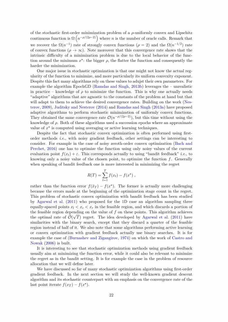
Despite the fact that stochastic convex optimization is often performed using first-order methods i.e., with noisy gradient feedback, other settings can be interesting toconsider. For example in the case of noisy zeroth-order convex optimization (Bach andPerchet, 2016) one has to optimize the function using only noisy values of the currentevaluation point f(xt) + ε. This corresponds actually to using “bandit feedback” i.e., toknowing only a noisy value of the chosen point, to optimize the function f . Generallywhen speaking of bandit feedback one is more interested in minimizing the regret

R(T ) =T∑t=1

f(xt)− f(x?) ,

rather than the function error f(xT ) − f(x?). The former is actually more challengingbecause the errors made at the beginning of the optimization stage count in the regret.This problem of stochastic convex optimization with bandit feedback has been studiedby Agarwal et al. (2011) who proposed for the 1D case an algorithm sampling threeequally-spaced points xl < xc < xr in the feasible region, and which discards a portion ofthe feasible region depending on the value of f on these points. This algorithm achievesthe optimal rate of O(

√T ) regret. The idea developed by Agarwal et al. (2011) have

similarities with the binary search, except that they discard a quarter of the feasibleregion instead of half of it. We also note that some algorithms performing active learningor convex optimization with gradient feedback actually use binary searches. It is forexample the case of (Burnashev and Zigangirov, 1974) on which the work of Castro andNowak (2006) is built.

It is interesting to see that stochastic optimization methods using gradient feedbackusually aim at minimizing the function error, while it could also be relevant to minimizethe regret as in the bandit setting. It is for example the case in the problem of resourceallocation that we will define later.

We have discussed so far of many stochastic optimization algorithms using first-ordergradient feedback. In the next section we will study the well-known gradient descentalgorithm and its stochastic counterpart with an emphasis on the convergence rate of thelast point iterate f(xT )− f(x?).

22

2.4 Gradient Descent and continuous models (Chapter 4)

Consider the minimization problem of a convex and L-smooth4 function f : Rd → R:

minx∈Rd

f(x) . (3)

There exist plenty of methods to provide solutions to this problem. The most usedones are likely first-order methods i.e., methods using the first derivative, as gradientdescent, to minimize the function f . These methods are very popular today because ofthe constantly increasing sizes of the datasets, which rule out second-order methods (asNewton’s method).

The gradient descent algorithm starts from a point x0 ∈ Rd and iteratively constructsa sequence of points approaching x? = arg minx∈Rd f(x) based on the following recursion:

xk+1 = xk − η∇f(xk) with η = 1/L . (4)

Even if there exists a classical proof of convergence of this gradient descent algorithm,see (Bertsekas, 1997) for instance, we propose here an alternative proof based on theanalysis of the continuous counterpart of (4). Consider a regular function X : R+ → Rdsuch that X(kη) = xk for all k ≥ 0. Using a Taylor expansion of order 1 gives

xk+1 − xk = −η∇f(xk)X((k + 1)η)−X(kη) = −η∇f(X(kη))

ηX(kη) + O(η) = −η∇f(X(kη))X(kη) = −∇f(X(kη)) + O(1) ,

suggesting to consider the following Ordinary Differential Equation (ODE)

X(t) = −∇f(X(t)), t ≥ 0 . (5)

The ODE (5), which is the continuous counterpart of the discrete scheme (4), can beeasily analyzed by considering the following energy function, where f? = f(x?),

E(t) , t(f(X(t))− f?) + 12 ‖X(t)− x?‖2 .

Differentiating E and using the convexity of f give, for all t ≥ 0,

E ′(t) = f(X(t))− f? + t〈∇f(X(t)), X(t)〉+ 〈X(t)− x?, X(t)〉= f(X(t))− f? − t ‖∇f(X(t))‖2 − 〈∇f(X(t)), X(t)− x?〉≤ −t ‖∇f(X(t))‖2 ≤ 0 .

Consequently E is non-increasing and for all t ≥ 0, we have t(f(X(t)) − f?) ≤ E(t) ≤E(0) = 1

2 ‖X(0)− x?‖2. This gives the following proposition

Proposition 1. Let X : Rd → R be given by (5). Then for all t > 0

f(X(t))− f? ≤ 12t ‖X(0)− x?‖2 .

4A L-smooth function is a function whose gradient is L-Lipschitz-continuous.

23

We now want to transpose this short and elegant analysis to the discrete setting. Wepropose therefore to introduce the following discrete energy function

E(k) = kη (f(xk)− f(x?)) + 12 ‖xk − x

?‖2 .

First state and prove the following lemma.

Lemma 1. If xk and xk+1 are two iterates of the gradient descent scheme (4), it holdsthat

f(xk+1) ≤ f(x?) + 1η〈xk+1 − xk, x? − xk〉 −

12η ‖xk+1 − xk‖2 . (6)

Proof. We have xk+1 = xk − η∇f(xk) which gives ∇f(xk) = xk − xk+1

η.

The descent lemma (Nesterov, 2004, Lemma 1.2.3) and then the convexity of f give

f(xk+1) ≤ f(xk) + 〈∇f(xk), xk+1 − xk〉+ L

2 ‖xk+1 − xk‖2

≤ f(x?) + 〈∇f(xk), xk − x?〉+ 〈xk − xk+1

η, xk+1 − xk〉+ 1

2η ‖xk+1 − xk‖2

≤ f(x?) + 1η〈xk+1 − xk, x? − xk〉 −

12η ‖xk+1 − xk‖2 .

This second lemma is immediate and well-known

Lemma 2. If xk and xk+1 are two iterates of the gradient descent scheme with have

f(xk+1) ≤ f(xk)−12η ‖xk+1 − xk‖2 . (7)

Proof. The descent lemma (Nesterov, 2004, Lemma 1.2.3) gives

f(xk+1) ≤ f(xk) + 〈∇f(xk), xk+1 − xk〉+ L

2 ‖xk+1 − xk‖2

≤ f(xk)− 12η ‖xk+1 − xk‖2 .

Let us now analyze E(k). Multiplying Equation (6) by 1/(k+ 1) and Equation (7) byk/(k + 1) we obtain

f(xk+1) ≤ k

k + 1f(xk) + 1k + 1f(x?)− 1

2η ‖xk+1 − xk‖2

+ 1k + 1

1η〈xk+1 − xk, x? − xk〉

f(xk+1)− f(x?) ≤ k

k + 1 (f(xk)− f(x?))− 12η ‖xk+1 − xk‖2

+ 1k + 1

1η〈xk+1 − xk, x? − xk〉

(k + 1)η (f(xk+1)− f(x?)) ≤ kη (f(xk)− f(x?))− k + 12 ‖xk+1 − xk‖2 + 〈xk+1 − xk, x? − xk〉 .

We note Ak , (k + 1)η (f(xk+1)− f(x?))− kη (f(xk)− f(x?)). It gives

Ak ≤ −k + 1

2 ‖xk+1 − xk‖2 + 〈xk+1 − xk, x? − xk〉

24

≤ k + 12

(−‖xk+1 − x?‖2 − ‖xk − x?‖2 + 2〈xk+1 − x?, xk − x?〉

)+ 〈xk+1 − x?, x? − xk〉+ ‖xk − x?‖2

≤ −k + 12 ‖xk+1 − x?‖2 −

k − 12 ‖xk − x?‖2 + k〈xk+1 − x?, xk − x?〉 .

Thus we have

E(k + 1) = (k + 1)η (f(xk+1)− f(x?)) + 12 ‖xk+1 − x?‖2

≤ kη (f(xk)− f(x?))− k

2 ‖xk+1 − x?‖2 −k

2 ‖xk − x?‖2 + 1

2 ‖xk − x?‖2

+ k〈xk+1 − x?, xk − x?〉

≤ E(k)− k

2(‖xk+1 − x?‖2 + ‖xk − x?‖2 − 2〈xk+1 − x?, xk − x?〉

)≤ E(k)− k

2 ‖xk+1 − xk‖2 ≤ E(k) .

This shows that (E(k))k≥0 is non-increasing and consequently E(k) ≤ E(0) = 12 ‖x0 − x?‖2.

This allows us state the following proposition, which is the discrete analogous of Propo-sition 1.

Proposition 2. Let (xk)k∈N be given by (4) with f : Rd → R convex and L-smooth. Itholds that for all k ≥ 1,

f(xk)− f(x?) ≤ L

2k ‖x0 − x?‖2 .

With this simple example we have demonstrated the interest of using the continuouscounterpart of a discrete problem to gain intuition on a proof scheme for the originaldiscrete problem. Note that the discrete proof is more involved than the continuousone, and that will always be the case in this manuscript. One reason is that we cancompute the derivative of the energy function in the continuous case, whereas this isnot possible in the discrete setting. In order to circumvent this we can use the descentlemma (Nesterov, 2004, Lemma 1.2.3) which can be seen as a discrete derivative, but atthe price of additional terms and computations.

Following these ideas, Su et al. (2016) have recently proposed a continuous modelof the famous Nesterov accelerated gradient descent method (Nesterov, 1983). Nesterovaccelerated method is an improvement over the momentum method (Polyak, 1964) whichwas already an improvement over the standard gradient descent method, which actuallygoes back to Cauchy (1847). The idea behind the momentum method is to dampenoscillations by using a fraction of the past gradients into the update term. By doing that,the update uses an exponentially weighted average of all the past gradients and smooth thesequence of points since it will mainly keep the true direction of the gradient and discardthe oscillations. However, even if momentum experimentally fastens gradient descent, itdoes not improve its theoretical convergence rate given by Proposition 2, contrarily toNesterov’s accelerated method, which can be stated as followsxk+1 = yk − η∇f(yk) with η ≤ 1/L

yk = xk + k − 1k + 2(xk − xk−1)

. (8)

Nesterov’s method still uses the idea of momentum but together with a lookahead com-putation of the gradient, which leads to an improved rate of convergence:

25

Theorem 1. Let f be a convex and L-smooth function. Then Nesterov’s acceleratedgradient descent method satisfies for all k ≥ 1

f(xk)− f(x?) ≤ 2L ‖x0 − x?‖2

k2 .

This convergence rate which improves the one of Proposition 2 matches the lowerbound of (Nesterov, 2004, Theorem 2.1.7), but the proof is not very intuitive, nor theideas leading to scheme (8). The continuous scheme introduced by Su et al. (2016) providesmore intuition on the acceleration phenomenon by proposing to study the second-orderdifferential equation

X(t) + 3tX(t) +∇f(X(t)) = 0, t ≥ 0 .

The authors prove the following convergence rate for the continuous model:

for all t > 0, f(X(t))− f? ≤ 2 ‖X(0)− x?‖2

t2,

again by introducing an appropriate energy function, which they choose to be in thiscase E(t) = t2 (f(X(t))− f?) + 2‖X(t) + tX(t)/2 − x?‖2 and which they prove to benon-increasing.

After having investigated the gradient descent algorithm and some of its variants, anatural line of research is to consider the stochastic case. One important use case ofgradient descent is indeed machine learning, and more particularly deep learning, wherevariants of gradient descent are used to minimize the loss functions of neural networksand to learn the weights of these neurons. In deep learning applications, practitioners areusually interested in minimizing a function f of the form

f(x) = 1N

N∑i=1

fi(x) , (9)

where fi is associated with the i-th observation of the training set (of size N , usuallyvery large). Consequently computing the gradient of f is very costly since it requires tocompute the N gradients ∇fi. In order to accelerate training one usually uses stochasticgradient descent by approximating the gradient of f by ∇fi with i chosen uniformly atrandom between 1 and N . A compromise between this choice and the standard classicalgradient descent algorithm is to use “mini-batches” which are small sets of points in1, . . . , N to estimate the gradient:

∇f(x) ≈ 1M

M∑i=1∇fσ(i)(x) ,

where σ is a permutation of 1, . . . , N and M is the size of mini-batch. Both of thesechoices provide approximations g(x) of the true gradient ∇f(x), and since the pointsused to compute those approximations are chosen uniformly at random we have E [g(x)] =∇f(x). Using these stochastic approximations of ∇f(x) instead of the true gradient valuein the gradient descent algorithm leads to the “Stochastic Gradient Descent algorithm”(SGD), which has a more general formulation than the one derived above. SGD canindeed be used to deal with the minimization problem (3) with noisy evaluations of ∇ffor a wider class of functions than the ones of the form (9).

26

Obtaining convergence results for SGD is more challenging than for gradient descent,due to the stochastic uncertainties. In the case of SGD, the goal is to bound E [f(xk)]−f?because the sequence (xk)k≥0 is now stochastic. Convergence results in the case wheref is strongly convex are well-known (Nemirovski et al., 2009; Bach and Moulines, 2011)but convergence results in the convex case are not as common. Most of the convergenceresults in the convex case are indeed obtained for the Polyak-Ruppert averaging framework(Polyak and Juditsky, 1992; Ruppert, 1988) where instead of considering the last iteratexN , convergence rates are derived for the average xN defined as follows

xN = 1N

N∑k=1

xk .

Obtaining convergence rates in the case of averaging, as done by Nemirovski et al. (2009),is easier than obtaining non-asymptotic convergence rates for the last iterate. Indeed ifone is able to derive non-asymptotic rates for the last iterate, using Jensen inequalitydirectly gives the convergence results in the averaged setting. Note moreover that allthe algorithms presented in Section 2.3 do not consider the final iterate but rather someaveraged version of the previous iterates. To the author’s knowledge there is no generalconvergence results in the convex and smooth case for SGD. One of the only results forthe last iterate is obtained by Shamir and Zhang (2013) who assume compactness of theiterates, a strong assumption. Moreover Bach and Moulines (2011) conjectured that theoptimal convergence rate of SGD in the convex case is O(k−1/3), which we disprove inChapter 4.

3 Outline and contributionsThis thesis is be divided into four chapters, each corresponding to one distinct problem.Each of these chapters led to a publication or a pre-publication. We decided to group thefirst three chapters in a first part about sequential learning, while the last chapter willbe the object of a second part, which is quite different, about stochastic optimization.Chapter 3 can be seen as a link between both parts.

We present in the following a summary of our main contributions and of the resultsobtained in the next chapters of this thesis. The goal of the following sections is tosummarize our results, not to give exhaustive statements of all the hypotheses and theo-rems. We tried to keep this part easily readable and refer the reader to the correspondingchapters to obtain all the necessary details.

3.1 Part I Chapter 1

In this chapter we study the problem of stochastic contextual bandits with regularization,with a nonparametric point of view. More precisely, as introduced in Section 2.1, weconsider a set of K ∈ N∗ arms with reward functions µk : X → R corresponding tothe conditional expectations of the rewards of each arm given the context values drawnuniformly at random from a set X = [0, 1]d. We assume that each of these functions isβ-Hölder continuous and, denoting p : X → ∆K the occupation measure of each arm weaim at minimizing the loss function

L(p) =∫X〈µ(x), p(x)〉+ λ(x)ρ(p(x)) dx ,

27

where ∆K is the unit simplex of RK , ρ : ∆K → R is a convex regularization function(typically the entropy) and λ : X → R is a regularization parameter function. Both aresupposed to be differentiable and chosen by the decision maker.

We denote by p? the optimal proportion function

p? = arg infp∈f :X→∆K

L(p) ,

and we design in Chapter 1 an algorithm whose aim is to produce after T iterations aproportion function (or occupation measure) pT minimizing the regret

R(T ) = E [L(pT )]− L(p?) .

Since pT is actually the vector of the empirical frequencies of each arm, R(T ) has to beconsidered as a cumulative regret.

We analyze the proposed algorithm to obtain upper bounds on this regret underdifferent assumptions. The algorithm we propose uses a binning of the context space andsolves separately a convex optimization problem on each bin.

We begin by establishing slow rates for constant λ under mild assumptions. We call“slow rates” convergence results slower than O(T−1/2) (and conversely by “fast rates”convergence bounds faster than O(T−1/2)).

Theorem 2. If λ is constant and ρ is a convex and smooth function we obtain thefollowing slow bound on the regret after T ≥ 1 samples:

R(T ) ≤ O

( T

log(T )

)− β2β+d

.

If we further assume that ρ is strongly convex and that the minimum of the lossfunction on each bin is reached far from the boundaries of ∆K , then we can obtain fasterrates.

Theorem 3. If λ is constant and ρ is a strongly convex and smooth function and if Lreaches its minimum far5 from ∂∆K , we obtain the following fast bound on the regretafter T ≥ 1 samples:

R(T ) ≤ O

( T

log(T )2

)− 2β2β+d

.

However this fast rate hides a multiplicative constant involving 1/λ and 1/η (whereη is the distance of the optimum to ∂∆K) which can be arbitrarily large. We considertherefore also the case where λ is a function of the context value, meaning that the agentcan modulate the weight of the regularization depending on the context. In that case thedistance of the optimum to the boundary will also depend on the context value and wedefine the function η as follows

η(x) := dist(p?(x), ∂∆K) ,

where p?(x) ∈ ∆K is the point where (p 7→ 〈µ(x), p〉+ λ(x)ρ(p)) reaches its minimum. Inorder to remove the dependency in λ and η in the bound of the regret, while achievingfaster rates than the ones of Theorem 2, we have to consider an additional assumptionlimiting the possibility for λ and η to take small values (that lead to large constant factorsin Theorem 3). This is classical in nonparametric estimation and we make therefore thefollowing assumption known as a “margin condition”:

5See Section 1.4.2 for a more precise statement.

28

Assumption 1. There exist δ1 > 0, δ2 > 0, α > 0 and Cm > 0 such that

∀δ ∈ (0, δ1], PX(λ(x) < δ) ≤ Cmδ6α and ∀δ ∈ (0, δ2], PX(η(x) < δ) ≤ Cmδ6α .

This condition involves a margin parameter α that controls the difficulty of the prob-lem and allows us to obtain intermediate convergence rates that interpolate perfectlybetween the slow and the fast rates, without any dependency in η or λ.

Theorem 4. If ρ is a convex function then with a margin condition of parameter α ∈ (0, 1)we obtain the following rates for the regret after T ≥ 1 samples

R(T ) = O

( T

log2(T )

)− β2β+d (1+α)

.

We can wonder whether the convergence results obtained in the three theorems pre-sented above are optimal or not. Note first that the convergence rates we obtain are clas-sical in nonparametric estimation (Tsybakov, 2008). Moreover we derive a lower boundon the considered problem showing that the fast upper bound of Theorem 3 is optimalup to the logarithmic terms.

Theorem 5. For any algorithm with bandit input and output pT , for ρ that is stronglyconvex and µ β-Hölder, there exists a universal constant C such that

infp

supρ,µ

E[L(pT )]− L(p?)

≥ C T−

2β2β+d .

We conclude the chapter with numerical experiments on synthetic data to illustrateempirically our convergence results.

3.2 Part I Chapter 2

In this chapter we consider the problem of actively estimating a design matrix for linearregression, detailed in Section 2.2. Our goal is to obtain the most precise estimate of theparameter β? of the linear regression i.e., to produce with T samples an estimate β whichminimizes the `2-norm E[‖β? − β‖2]. If we introduce the matrix

Ω(p) =K∑k=1

(pk/σ2k )XkX

>k ,

for p ∈ ∆K , our problem corresponds to minimizing the trace of its inverse (which is thecovariance matrix), since

E[‖β − β?‖2

]= 1TTr(Ω(p)−1) .

This shows that our problem consists actually in performing A-optimal design in anonline manner. More precisely we introduce the loss function L(p) = Tr(Ω(p)−1) which isstrictly convex and which admits therefore a minimum p?. Our goal is then to minimizethe regret of the algorithm i.e., the gap between the achieved loss and the best loss thatcan be reached. We define therefore

R(T ) = E[‖β − β?‖2

]−min

algoE[‖β(algo) − β?‖2

]= 1T

(E [L(pT )]− L(p?)) .

29

Note that, similarly to Section 3.1, R(T ) is again not a simple regret but a cumulativeone.

In Chapter 2 we construct an active learning algorithm building on the work (Berthetand Perchet, 2017) to solve the problem of online A-optimal design. We obtain a concen-tration result on the variances of subgaussian random variables and we use it to analyzeour algorithm. Note that in the case where K < d, the matrix op is degenerate andhence the regret is linear, unless we restrict the analysis to the subspace spanned by thecovariates. Therefore we consider from now on that K ≥ d.

We consider two cases in our analysis. The first one handles the case where the numberK of possible covariates is equal to their dimension d. In this case we know that all thecovariates have to be sampled. The control of the number of samples of each arm thatcan be sampled is crucial and our algorithm uses a well-designed pre-sampling phase toforce the loss function to be locally smooth, which helps us to achieve a fast convergenceresult.

Theorem 6. In the case where K = d we obtain the following fast rate for all T ≥ 1

R(T ) = O(

log2(T )T 2

).

We need to mention that this fast rate is hard to obtain. In Section 2.3 we proposeindeed a naive algorithm for our problem using UCB-like techniques and we prove that itonly achieves O(T−3/2) regret.

In the second case where K > d the problem is much more difficult. Different situa-tions can arise and the optimal allocation p? can be reached either by not sampling somecovariate points, or by sampling all of them. Finding out which is the optimal scenario isa hard problem justifying the worse upper bound we obtain in this case

Theorem 7. In the case where K > d we obtain the following upper-bound on the regretfor all T ≥ 1

R(T ) = O( log(T )T 5/4

).

This upper bound is not tight as we were able to derive the following lower bound inthe case K > d:

Theorem 8. For any algorithm, there exists a set of parameters such that R(T ) & T−3/2.

The numerical experiments we perform at the end of Chapter 2 illustrate the fact thatthe case where K > d is more challenging and that the optimal convergence rate certainlylies between T−5/4 and T−3/2.

3.3 Part I Chapter 3

In this chapter we study a problem that lies at the boundary between sequential learningand stochastic convex optimization. We consider the problem of resource allocation whichwe formulate as follows. A decision maker has access to a set of K different resources,on which he can allocate an amount xk, generating a reward fk(xk). At each time stepthe agent can only allocate a fixed budget, meaning that ∑K

k=1 xk = 1. Consequently thedecision maker receives at each time step t ∈ 1, . . . , T the reward

F (x(t)) =K∑k=1

fk(x(t)k ) with x(t) = (x(t)

1 , . . . , x(t)K ) ∈ ∆K ,

30

that has to be maximized. Noting x? ∈ ∆K the optimal allocation maximizing F , the goalof the decision maker can be equivalently restated as minimizing the cumulative regret

R(T ) = F (x?)− 1T

T∑t=1

K∑k=1

fk(x(t)k ) = max

x∈∆KF (x)− 1

T

T∑t=1

F (x(t)) .

Resource allocation has been considered in many fields for centuries and we make thereforea classical assumption that goes back to Smith (1776) which is known as the “diminishingreturns” assumption that postulates that the reward functions are concave. In this chapterwe assume that the decision maker has also access at each time step to a noisy value of∇F (x(t)) in order to perform minimization, which makes us compete against other first-order stochastic optimization algorithms.

In order to measure the complexity of the problem at hand we make an additionalassumption that is based on the Łojasiewicz inequality (Łojasiewicz, 1965), which is aweaker form of uniform convexity. The precise assumption is explained in details inSection 3.2.3 but we state here a particular case for simplicity

Assumption 2. For all k ∈ 1, · · · ,K, fk is ρ-uniformly concave.

With this assumption we say that we verify “inductively” the Łojasiewicz inequalitywith parameter β = ρ

ρ−1 , see Proposition 3.5. The goal of Chapter 3 is to design analgorithm adaptive to the unknown Łojasiewicz exponent and which minimizes the regret.Going back to the discussion of Section 2.3 we are interested in the more challenging taskof regret minimization instead of function error minimization, which actually rules outthe algorithms proposed by Juditsky and Nesterov (2014) or Ramdas and Singh (2013a),which only achieve linear regret.

The algorithm we design uses as its central ingredient the concept of binary search. Letus sketch it in the simpler case of K = 2 resources. In that case F (x) = f1(x1)+f2(x2) =f1(x1) + f2(1− x1) , f1(x) + f2(1− x) can be seen as a function defined over [0, 1]. Theidea of the algorithm is to sample each query point x a sufficient number of times toobtain with high confidence the sign of ∇F (x), which will tell whether x lies to the rightor to the left of x?. We run therefore a binary search by discarding half of the searchinterval at each epoch. Since points that are far from x? will be sampled a small numberof times, because the sign of their gradient will be quickly found, this algorithm achievessublinear regret. It is easy to show that our algorithm achieves O(T−1) regret in thestrongly concave case, reaching therefore the classical rate of stochastic optimization ofstrongly convex functions. In the more general case we obtain the following rate, usingimbricated binary searches.

Theorem 9. Assume that our problem satisfies inductively the Łojasiewicz inequality withβ ≥ 1. Then we obtain the following bound on the regret after T ≥ 1 samples

in the case β > 2, E[R(T )] ≤ O(K

log(T )log2(K)

T

);

in the case β ≤ 2, E[R(T )] ≤ O

K (log(T )log2(K)+1

T

)β/2 .

Note that in the case of Assumption 2, β = ρ/(ρ− 1) ≤ 2 and we obtain a bound onthe regret which scales as T−ρ/(2ρ−2), which is exactly what was obtained by Ramdas andSingh (2013a,b) and Juditsky and Nesterov (2014), but this time for the regret and not

31

for the function error. As in the previous chapters we also analyze the optimality of theupper bound obtained in the previous theorem. We prove the following lower bound inthe case where β ∈ [1, 2]

Theorem 10. For any algorithm there exists a pair of concave non-decreasing functionsf1 and f2 such that

E [R(T )] ≥ cβT−β2 ,

where cβ > 0 is some constant independent of T .

This result proves that our upper bound is minimax optimal up to the logarithmicterms. We finally illustrate these theoretical findings with numerical experiments per-formed on synthetic datasets.

Moreover we also demonstrate how our setting can generalize the case of Multi-Armed Bandit by considering linear resources. In Section 3.3.5 we retrieve the classicallog(T )/(T∆) rate of Multi-Armed Bandit algorithms.

3.4 Part II Chapter 4

In this chapter we analyze the widely-used algorithm of Stochastic Gradient Descent(SGD) that was discussed in Section 2.4. Let f : Rd → R the objective function tominimize. We will assume that f is continuously differentiable and smooth, and that wedo not have access to ∇f(x) but rather to unbiased estimates given by H(x, z) where zis a realization of a random variable Z on Z of density µZ verifying

∀x ∈ Rd,∫

ZH(x, z)dµZ(z) = ∇f(x) .

We then define SGD as follows

Xn+1 = Xn − γ(n+ 1)−αH(Xn, Zn+1) , (10)

where γ > 0 is the initial stepsize, α ∈ [0, 1] allows the use of decreasing stepsizes and(Zn)n∈N is a sequence of independent random variables distributed from µZ. As ex-plained in Section 2.4 we want to study SGD by performing the analysis of its continuouscounterpart that we show to be the following time-inhomogeneous Stochastic DifferentialEquation (SDE)

dXt = −(γα + t)−α∇f(Xt)dt+ γ1/2α Σ(Xt)1/2dBt , (11)

where γα = γ1/(1−α), Σ(x) = µZ(H(x, ·)−∇f(x)H(x, ·)−∇f(x)>) and (Bt)t≥0 is ad-dimensional Brownian motion.

One of the contributions of Chapter 4 is to propose a new method to derive the conver-gence rates of SGD, by analyzing the corresponding SDE. We argue that this method issimpler than existing ones. We demonstrate first its efficiency on the case of strongly con-vex functions. The method we propose consists in using an appropriate energy functionto obtain convergence results in the continuous case, and then to adapt the proof to thediscrete case by using similar techniques. The continuous case gives therefore intuition.For example we are able to prove the following result in the strongly convex case

Theorem 11. If f is a strongly convex and smooth function then the SGD scheme (10)with decreasing stepsizes of parameter α ∈ (0, 1] has the following convergence speed forany N ≥ 1,

E[‖XN − x?‖2

]≤ CN−α .

32

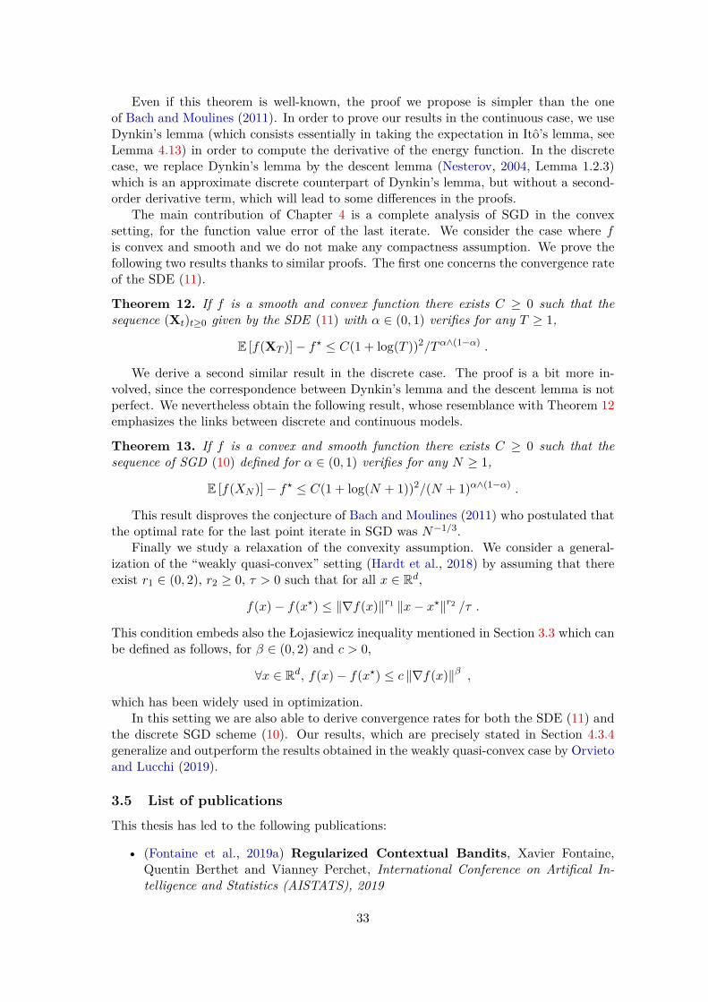
Even if this theorem is well-known, the proof we propose is simpler than the oneof Bach and Moulines (2011). In order to prove our results in the continuous case, we useDynkin’s lemma (which consists essentially in taking the expectation in Itô’s lemma, seeLemma 4.13) in order to compute the derivative of the energy function. In the discretecase, we replace Dynkin’s lemma by the descent lemma (Nesterov, 2004, Lemma 1.2.3)which is an approximate discrete counterpart of Dynkin’s lemma, but without a second-order derivative term, which will lead to some differences in the proofs.

The main contribution of Chapter 4 is a complete analysis of SGD in the convexsetting, for the function value error of the last iterate. We consider the case where fis convex and smooth and we do not make any compactness assumption. We prove thefollowing two results thanks to similar proofs. The first one concerns the convergence rateof the SDE (11).

Theorem 12. If f is a smooth and convex function there exists C ≥ 0 such that thesequence (Xt)t≥0 given by the SDE (11) with α ∈ (0, 1) verifies for any T ≥ 1,

E [f(XT )]− f? ≤ C(1 + log(T ))2/Tα∧(1−α) .

We derive a second similar result in the discrete case. The proof is a bit more in-volved, since the correspondence between Dynkin’s lemma and the descent lemma is notperfect. We nevertheless obtain the following result, whose resemblance with Theorem 12emphasizes the links between discrete and continuous models.

Theorem 13. If f is a convex and smooth function there exists C ≥ 0 such that thesequence of SGD (10) defined for α ∈ (0, 1) verifies for any N ≥ 1,

E [f(XN )]− f? ≤ C(1 + log(N + 1))2/(N + 1)α∧(1−α) .

This result disproves the conjecture of Bach and Moulines (2011) who postulated thatthe optimal rate for the last point iterate in SGD was N−1/3.

Finally we study a relaxation of the convexity assumption. We consider a general-ization of the “weakly quasi-convex” setting (Hardt et al., 2018) by assuming that thereexist r1 ∈ (0, 2), r2 ≥ 0, τ > 0 such that for all x ∈ Rd,

f(x)− f(x?) ≤ ‖∇f(x)‖r1 ‖x− x?‖r2 /τ .

This condition embeds also the Łojasiewicz inequality mentioned in Section 3.3 which canbe defined as follows, for β ∈ (0, 2) and c > 0,

∀x ∈ Rd, f(x)− f(x?) ≤ c ‖∇f(x)‖β ,

which has been widely used in optimization.In this setting we are also able to derive convergence rates for both the SDE (11) and

the discrete SGD scheme (10). Our results, which are precisely stated in Section 4.3.4generalize and outperform the results obtained in the weakly quasi-convex case by Orvietoand Lucchi (2019).

3.5 List of publications

This thesis has led to the following publications:

• (Fontaine et al., 2019a) Regularized Contextual Bandits, Xavier Fontaine,Quentin Berthet and Vianney Perchet, International Conference on Artifical In-telligence and Statistics (AISTATS), 2019

33

• (Fontaine et al., 2019b) Online A-Optimal Design and Active Linear Re-gression, Xavier Fontaine, Pierre Perrault, Michal Valko and Vianney Perchet,submitted

• (Fontaine et al., 2020b) An adaptive stochastic optimization algorithm forresource allocation, Xavier Fontaine, Shie Mannor and Vianney Perchet, Inter-national Conference on Algorithmic Learning Theory (ALT), 2020

• (Fontaine et al., 2020a) Convergence rates and approximation results forSGD and its continuous-time counterpart, Xavier Fontaine, Valentin De Bor-toli and Alain Durmus, submitted.

In addition, the author also participated in the following publication that is not dis-cussed in the present thesis:

• (De Bortoli et al., 2020)Quantitative Propagation of Chaos for SGD in WideNeural Networks, Valentin de Bortoli, Alain Durmus, Xavier Fontaine and UmutŞimşekli, Advances in Neural Information Processing Systems, 2020.

In what follows we made the choice to postpone the long proofs to the end of eachchapter in order to improve readability.

34

Introduction en français

1 MotivationsLes problèmes d’optimisation sont très fréquents aujourd’hui et peuvent servir par

exemple à utiliser au mieux notre temps, à minimiser la durée d’un trajet, ou à maximiserle gain d’un produit financier avec des contraintes de risque. Les problèmes d’optimisationavec ou sans contraintes sont présents dans de nombreux domaines des mathématiquescomme la théorie du contrôle, la recherche opérationnelle, la finance, le transport optimalou l’apprentissage automatique. Nous nous intéresserons principalement dans cette thèseaux problèmes d’optimisation qui apparaissent en apprentissage automatique. Malgré sesdomaines nombreux et variés d’application, comme le traitement automatique du langage,l’analyse d’image, la publicité ciblée, etc., tous les algorithmes d’apprentissage reposenten effet sur le concept d’optimisation, et plus précisément sur l’optimisation stochas-tique. Les algorithmes d’apprentissage automatique sont généralement analysés à traversle formalisme de l’apprentissage statistique, dont le but est d’estimer (ou d’apprendre) lameilleure fonction de prédiction sur une tâche précise à l’aide de données, c’est-à-dire detrouver la fonction la plus probable qui corresponde aux données. Pour ce faire on utilisesouvent des techniques d’optimisation, par exemple pour minimiser une fonction de perte,pour trouver les bons hyperparamètres ou pour maximiser un gain moyen.

Dans cette thèse nous nous concentrons sur l’étude d’une classe spécifique de problèmesd’apprentissage statistique où les données sont obtenues et traitées à la volée, et qui estconnue sous le nom d’apprentissage séquentiel, ou apprentissage en ligne (Shalev-Shwartz,2012), en opposition à l’apprentissage hors-ligne où les données ont été récupérées avantl’apprentissage. La principale difficulté de l’apprentissage séquentiel est précisément le faitque l’agent que l’on considère doit construire une fonction de prédiction sans connaîtretoutes les données. C’est pour cela que les algorithmes en ligne sont généralement moinsperformants que les algorithmes hors-ligne pour lesquels l’agent a accès à l’ensemble desdonnées. Les situations d’apprentissage en ligne peuvent cependant avoir aussi des avan-tages quand l’agent joue un rôle actif dans le processus de collection des données. Dansce domaine de l’apprentissage automatique, que l’on appelle généralement apprentissageactif (Settles, 2009), l’agent est capable de choisir quelles données collecter et quellesdonnées labelliser. Faire partie intégrante du processus de sélection des données peutaméliorer la performance de l’algorithme d’apprentissage puisque l’agent choisira les don-nées qui apporteront le plus d’information. Dans les problèmes d’apprentissage séquentielon considère donc un agent qui doit prendre des décisions à chaque pas de temps, sachantque les actions qu’il aura choisies pourront avoir une influence sur la suite du processusd’apprentissage. Ainsi dans les problèmes de bandits (Bubeck et Cesa-Bianchi, 2012), quisont une façon simple de modéliser les prises de décision avec incertitude, l’agent doit

35

sélectionner une action (que l’on appelle généralement “bras”) parmi plusieurs dans lebut de maximiser son gain. Pour atteindre son but l’agent doit donc faire des choix, parexemple sélectionner le meilleur bras actuel, ou bien en choisir un autre afin d’explorerles différentes options à sa disposition et ainsi obtenir des informations sur celles-ci. Cecompromis entre l’exploitation des données et leur exploration est une des principales diffi-cultés des problèmes liés aux bandits. Dans les trois premiers chapitres de cette thèse nousallons étudier des problèmes d’apprentissage séquentiel ou actif où ce genre de compromisest très présent. Notre but sera toujours de minimiser une quantité, que l’on nomme “re-gret” et qui quantifie la différence entre la meilleure stratégie qu’aurait choisie un agentomniscient et la stratégie effectivement adoptée.

Les problèmes d’optimisation que l’on traite en apprentissage automatique ont géné-ralement la particularité de concerner des fonctions qui sont inconnues ou bruitées. Parexemple, dans le cas classique des bandits stochastiques (Lai et Robbins, 1985; Auer et al.,2002) on veut maximiser une récompense qui dépend des distributions de probabilité desbras, qui sont inconnues. Pour en savoir davantage sur ces distributions l’agent reçoit àchaque pas de temps un retour d’information, ou “feedback” (typiquement la récompensedu bras choisi) qui sera utilisé pour prendre les décisions suivantes. Dans les problèmesde bandits, on parle d’information “limitée” (ou de type bandit), en opposition à l’in-formation “complète” obtenue quand les récompenses de tous les bras (et pas seulementde celui qui a été choisi) sont dévoilées à l’agent. En outre, la difficulté des problèmesde bandits n’est pas uniquement due à l’information limitée mais aussi à son caractèrebruité : les récompenses des bras sont effet des valeurs bruitées des moyennes de chaquebras. C’est aussi le cas pour l’algorithme de Descente de Gradient Stochastique (SGDen anglais) (Robbins et Monro, 1951) qui sert à minimiser une fonction différentiable aumoyen des valeurs bruitées de son gradient. Du fait de l’aléatoire inhérent aux problèmesd’apprentissage on utilise donc en apprentissage automatique des méthodes d’optimisa-tion stochastique, qui consistent en l’optimisation de fonctions dont les valeurs dépendentde variables aléatoires. Puisque l’on travaille avec des fonctions aléatoires, les résultatsque nous obtiendront seront donc généralement énoncés en espérance ou avec grandeprobabilité.

Une des caractéristiques principales d’un algorithme d’optimisation (en plus de réalisereffectivement sa tâche de minimisation) est la vitesse à laquelle il atteint le minimum, oubien la précision qu’il peut garantir après un certain nombre d’itérations, ou avec unbudget fixé. Par exemple l’objectif des algorithmes de bandits est d’obtenir un regretsous-linéaire en T (l’horizon de temps de l’algorithme), et l’objectif de l’algorithme SGDest de borner E[f(xn)]−minx∈Rd f en fonction du nombre d’itérations n. Il faut en effetque les méthodes d’apprentissage automatique soient efficaces et précises, c’est-à-dire queles algorithmes d’optimisation qu’elles utilisent doivent converger rapidement. Obtenirdes vitesses de convergence pour les algorithmes que l’on étudie ici sera l’un des objectifsthéoriques majeurs de cette thèse. En outre, après avoir obtenu une borne de convergenceil faut se demander si cette vitesse peut être améliorée, soit grâce à une analyse plus précisede l’algorithme, soit par un meilleur algorithme pour le problème que l’on considère. Ilexiste deux réponses à cette question. La première réponse est évidente et consiste àcomparer les performances obtenues avec celles d’autres méthodes de la littérature. Ladeuxième réponse consiste à trouver une “borne inférieure” pour le problème, c’est-à-direune vitesse de convergence qui ne peut pas être battue. Si cette borne inférieure coïncideavec la vitesse de convergence de l’algorithme (appelée aussi “borne supérieure”) on ditque l’algorithme est “min-max optimal”, c’est-à-dire que l’on ne peut pas faire mieux.Dans ce manuscrit nous nous efforcerons dès que possible de comparer nos résultats avec

36

l’état de l’art et d’établir des bornes inférieures, afin de pouvoir avoir un avis sur lapertinence de nos algorithmes.

Pour obtenir des vitesses de convergence en optimisation il est important de s’inté-resser à la complexité du problème considéré. Plus le problème est complexe (ou moinsil est précis), plus les algorithmes seront lents. Par exemple, il est bien plus compliquéde minimiser une fonction arbitraire sur Rd que de minimiser une fonction différentiableet fortement convexe. Dans cette thèse on caractérisera la complexité d’un problème pardes mesures de complexité des fonctions que l’on considère : plus les fonctions serontrégulières, plus le problème sera facile. C’est pourquoi chaque chapitre débutera par unensemble d’hypothèses qui permettront à la fois de trouver une solution au problème etd’obtenir des vitesses de convergence. Nous verrons comment un changement de ces hy-pothèses modifiera les vitesses convergence obtenues. Par exemple dans les Chapitres 3et 4 nous obtiendrons des vitesses de convergence pour des algorithmes d’optimisationstochastique qui dépendront de l’exposant dans une inégalité de Łojasiewicz (Łojasie-wicz, 1965; Karimi et al., 2016). Nous verrons que des variations de cet exposant fontaugmenter ou baisser la complexité du problème, et donc les vitesses de convergence as-sociées. Une difficulté que nous rencontrerons dans ce manuscrit est due au fait que lesproblèmes que l’on étudie ne vérifient pas toujours ce genre d’hypothèses de régularité. Lesproblèmes réels ou les applications pratiques ne concernent en effet pas toujours des fonc-tions lisses ou convexes. Ainsi, les algorithmes d’optimisation stochastique tels que SGDont souvent des garanties de convergence (Bach et Moulines, 2011) dans le cas convexe(ou même fortement convexe), alors que très peu de résultats existent dans le cas nonconvexe, qui demeure néanmoins la situation la plus fréquente, par exemple en apprentis-sage profond. Un des défis de cette thèse sera donc de traiter ces cas. Notons par ailleursque la performance réelle d’un algorithme d’optimisation peut être bien meilleure que savitesse théorique. C’est typiquement le cas des algorithmes d’optimisation stochastiquementionnés plus haut qui sont beaucoup utilisés dans les réseaux de neurones sans avoirpour autant de garanties théoriques dans ce cas. Afin de pouvoir comparer les perfor-mances théoriques et pratiques de nos algorithmes nous présenterons dans cette thèse dessimulations numériques de nos méthodes.

Dans la suite de ce chapitre introductif nous présenterons les différents problèmes d’ap-prentissage séquentiel et d’optimisation que nous avons étudiés au cours de cette thèse,ainsi que les principaux outils mathématiques dont nous aurons besoin. Nous concluronspar des explications détaillées chapitre par chapitre des différentes contributions de cettethèse ainsi que par la liste des publications réalisées.

2 Présentation des problèmes étudiés

2.1 Bandits stochastiques contextuels (Chapitre 1)

Considérons un agent qui a accès à K ∈ N∗ bras qui sont chacun associés à unedistribution de probabilité νi, pour tout i ∈ 1, . . . ,K. Supposons qu’à chaque pas detemps t ∈ 1, . . . , T,1 l’agent peut choisir un bras it ∈ 1, . . . ,K et qu’il reçoit unerécompense Y (it)

t qui suit la distribution νit , loi de probabilité sur R+ d’espérance µit .L’agent a comme objectif de maximiser sa récompense totale ∑T

t=1 Y(it)t . Puisque les

récompenses sont aléatoires, nous allons plutôt tâcher de maximiser l’espérance de larécompense totale E

[∑Tt=1 µit

], où l’espérance porte sur l’aléa des décisions de l’agent.

1On suppose ici que l’horizon de temps T ∈ N∗ est connu, même si le “doubling-trick” (Auer et al.,1995) permettrait de s’affranchir de cette contrainte.

37

Ainsi nous sommes généralement intéressés par minimiser le regret (ou plus précisémentle “pseudo-regret”)

R(T ) = T max1≤i≤K

µi − E[T∑t=1

µit

]. (1)

C’est la formulation classique du problème de “bandits stochastiques multi-bras” (Bubecket Cesa-Bianchi, 2012) qui peut être résolu en utilisant l’algorithme bien connu UCB(Upper Confidence Bound) qui est dû à Lai et Robbins (1985).

Ce problème peut servir à modéliser de nombreuses situations où un compromis detype “exploration vs. exploitation” apparaît. C’est par exemple le cas des essais cliniquesou bien de la publicité en ligne où l’on veut trouver la meilleure publicité à afficher touten maximisant le nombre de clics. Cependant, le modèle décrit ci-dessus semble tropsimpliste pour proposer une solution adéquate aux problèmes mentionnés ci-dessus. Eneffet tous les patients, ou tous les internautes, ne se comportent pas de la même façon,et une publicité peut être appropriée pour quelqu’un et ne pas du tout être adaptéepour quelqu’un d’autre. Nous comprenons donc que le modèle évoqué plus haut est troprestrictif, et nous voyons en particulier que l’hypothèse que l’on a faite que chaque bras ia une espérance fixe µi n’est pas réaliste. C’est pour cela que nous devons introduire ceque l’on va appeler un ensemble de contextes X = [0, 1]d qui correspond aux différentsprofils possibles de patients ou d’internautes de notre problème. Chaque contexte x ∈ Xdonne les caractéristiques d’un utilisateur et nous allons donc maintenant supposer queles récompenses des K bras dépendent du contexte x. Ce problème est connu sous lenom de bandits avec information (Wang et al., 2005) ou de bandits contextuels (Langfordet Zhang, 2008) et modélise mieux les problèmes d’essais cliniques ou bien de publicitéciblée. Nous supposerons donc maintenant qu’à chaque pas de temps t ∈ 1, . . . , T l’agentobserve un contexte aléatoire Xt ∈ X et doit choisir un bras it dont la récompense Y (it)

dépendra du contexte Xt. Notons donc pour chaque bras i ∈ 1, . . . ,K, µi : X → Rl’espérance conditionnelle de la récompense du bras i par rapport à la variable de contexteX, qui est maintenant une fonction du contexte x :

E[Y (i) |X = x] = µi(x), pour tout x ∈ X .

Afin de tirer profit des contextes nous devons faire quelques hypothèses de régularité surles récompenses. Nous voulons en effet nous assurer qu’un bras donnera des récompensessimilaires pour deux variables de contexte proches (c’est-à-dire deux utilisateurs qui ontun profil semblable). Une façon de modéliser cette hypothèse naturelle est par exemple desupposer que les fonctions µi sont Lipschitz. Ce problème non paramétrique de banditscontextuels stochastiques a été étudié par Rigollet et Zeevi (2010) dans le cas de K = 2bras et ensuite par Perchet et Rigollet (2013) dans le cas général. Dans ces deux travaux,le but de l’agent est de trouver une stratégie π : X → 1, . . . ,K qui associe à un contexteun bras à tirer. Bien évidemment, comme dans le cas des bandits stochastiques classiques,l’action choisie dépendra de l’historique des précédents tirages, et la dépendance de π entemps est implicite. Nous pouvons maintenant définir la stratégie optimale π? ainsi quela fonction de récompense optimale µ? :

π?(x) ∈ arg maxi∈1,...,K

µi(x) et µ?(x) = maxi∈1,...,K

µi(x) .

Cela donne donc l’expression suivante pour le regret après T tirages

R(T ) =T∑t=1

E[µ?(Xt)− µπ(Xt)(Xt)

]. (2)

38

Même si les expressions (2) et (1) sont similaires, l’une des difficultés que l’on va rencontrerpour minimiser le regret est due au fait que l’on ne peut pas espérer obtenir plusieursrécompenses d’un bras pour une même valeur de contexte, puisque l’espace des contextesest indénombrable.

Une idée courante en statistiques non paramétriques (Tsybakov, 2008) pour estimerune fonction inconnue f sur X est d’utiliser des “régressogrammes”, qui sont des estima-teurs constants par morceaux de la fonction. Leur construction est similaire à celle d’his-togrammes, en partitionnant X en différents sous-ensembles et en approximant f par savaleur moyenne sur chacun des sous-ensembles de la partition. Les régressogrammes sontune alternative aux estimateurs de Nadaraya-Watson (Nadaraya, 1964; Watson, 1964) quieux utilisent des noyaux en guise de poids au lieu d’utiliser une partition de l’espace.

Une façon de résoudre le problème de bandits stochastiques contextuels consiste às’inspirer des régressogrammes et à partitionner l’espace de contextes X en différentssous-ensembles et à traiter le problème de bandits contextuels en différentes instancesindépendantes d’un problème de bandits sans contexte sur chacun des sous-ensembles dela partition. Cela peut-être réalisé au moyen d’un algorithme classique de bandits commeUCB ou ETC (Even-Dar et al., 2006) déployé indépendamment sur chaque sous-ensemble,ce qui donne lieu à une stratégie appelée “UCBogramme” (Rigollet et Zeevi, 2010). Unetelle stratégie n’est bien sûr possible que grâce à l’hypothèse de régularité que l’on a faiteprécédemment, et qui garantit que considérer une approximation constante des fonctionsµi ne crée par une erreur trop importante.

Au lieu de supposer que les fonctions µi sont Lipschitz, Perchet et Rigollet (2013) fontune hypothèse plus faible et très classique en estimation non paramétrique qui consisteà supposer que ces fonctions sont β-Hölder pour β ∈ (0, 1], c’est-à-dire que pour touti ∈ 1, . . . ,K et pour tout (x, y) ∈ X 2,

|µi(x)− µi(y)| ≤ L ‖x− y‖β .

Avec cette hypothèse ils obtiennent la borne classique suivante sur le regret R(T ) (où l’ona uniquement fait figurer la dépendance en T et pas celle en K)

R(T ) . T 1−β/(2β+d) .

Maintenant que l’on a obtenu une solution pour le problème de bandits stochastiquescontextuels nous pouvons nous demander s’il est toujours réaliste. Prenons en effet ànouveau l’exemple de la publicité en ligne. Supposons donc qu’une société de publicitéciblée souhaite utiliser des bandits contextuels pour définir sa stratégie. L’entreprise uti-lisait d’autres techniques précédemment et ne veut pas risquer de perdre trop d’argenten mettant en place sa nouvelle stratégie. Cette situation est une instance d’un pro-blème bien plus vaste que l’on appelle apprentissage par renforcement sécurisé (Garcíaet Fernández, 2015) et qui étudie les politiques d’apprentissage qui doivent respecter cer-taines contraintes de sécurité. Dans le cas spécifique des bandits, Wu et al. (2016) ontproposé un algorithme qu’ils ont appelé “UCB conservatif” qui consiste à faire tournerUCB tout en garantissant uniformément dans le temps que la récompense obtenue estplus grande qu’une portion 1− α de ce qui aurait été obtenu par la stratégie précédente.Pour obtenir ce résultat les auteurs ajoutent un bras supplémentaire correspondant àl’ancienne stratégie qu’ils tirent dès que la contrainte sur la récompense risque de ne plusêtre vérifiée. Dans le Chapitre 1 nous adoptons un autre point de vue sur ce problème : aulieu d’imposer une contrainte sur la récompense nous ajoutons un terme de régularisationpour forcer la nouvelle stratégie à être proche d’une stratégie déterminée à l’avance.

39

Dans les problèmes de bandits l’agent doit choisir des actions pour maximiser unerécompense mais il n’est généralement pas intéressé par les valeurs précises de chacun desbras. Estimer ces valeurs est un autre problème qui présente aussi un certain intérêt. Enrevanche les deux tâches d’estimation des moyennes des bras et de maximisation de larécompense totale ne sont pas compatibles puisque la tâche d’estimation nécessite aussid’échantillonner les bras sous-optimaux. Dans la section suivante nous nous intéresserons àune généralisation du problème d’estimation qui consiste à choisir intelligemment quel brastirer pour maximiser sa connaissance sur un paramètre inconnu (et qui peut typiquementêtre le vecteur des moyennes de chaque bras).

2.2 De la régression linéaire à la planification en ligne d’expériences defaçon optimale (Chapitre 2)

Considérons maintenant le problème de régression linéaire qui a déjà été très étudiéen apprentissage. Dans ce problème un agent a accès à un ensemble de données et delabels (xi, yi)i=1,...,n de n observations, où (xi, yi) ∈ Rp × R pour tout i ∈ 1, . . . , n.On suppose que ces points sont linéairement reliés :

∀i ∈ 1, . . . , n , yi = x>i β? + εi ,

où β? ∈ Rp est le vecteur des paramètres2 et ε = (ε1, . . . , εn)> est le vecteur de bruits quimodélise le terme d’erreur de la régression. Dans la suite de cette section nous supposeronsque le bruit est centré, c’est-à-dire que E [ε] = 0 et qu’il a une variance finie :

∀i ∈ 1, . . . , n , E[ε2i

]= σ2

i < +∞ .

Nous considérons tout d’abord le cas homoscédastique, c’est-à-dire que les variances σ2i

sont toutes supposées égales à σ2 pour chaque bras i ∈ 1, . . . , n. En régression linéaireon considère généralement la “matrice de design” X ainsi que le vecteur des observationsY définis ainsi

X =

· · · x>1 · · ·...

· · · x>n · · ·

∈ Rn×p et Y =

y1...yn

∈ Rn ,

ce qui donneY = Xβ? + ε .

L’objectif d’une régression linéaire est d’estimer le paramètre β? par un β ∈ Rp afin deminimiser l’erreur des moindres carrés L(β) entre les vraies valeurs observées yi et lesvaleurs prédites par le modèle linéaire X>i β :

L(β) =n∑i=1

(yi − x>i β)2 = ‖Y − Xβ‖22 .

Nous définissons donc l’estimateur optimal de β? comme β , arg minβ∈Rp L(β) et nousobtenons aisément la formule bien connue des moindres carrés

β = (X>X)−1X>Y ,

2On peut aussi ajouter un terme d’ordonnée à l’origine et supposer plutôt que yi = β?0 + x>i β? + εi,

avec β? ∈ Rp+1, mais cela ne changera pas grand chose à la discussion qui va suivre.

40

ce qui donne la relation suivante entre β? et β :

β = β? + (X>X)−1X>ε .

Nous pouvons donc définir la matrice de covariance de l’erreur d’estimation β? − β

Ω , E[(β? − β)(β? − β)>

]= σ2(X>X)−1 = σ2

(n∑i=1

xix>i

)−1

,

qui caractérise la précision de l’estimateur β.Comme nous l’avons montré ci-dessus, la régression linéaire est un problème simple et

bien compris aujourd’hui. Il peut toutefois être la brique de base de plusieurs problèmesplus complexes et plus intéressants. Supposons par exemple que les vecteurs x1, . . . , xnne sont plus fixes, mais qu’ils peuvent être choisis parmi un ensemble de points de tailleK > 0 X1, . . . , XK. L’agent doit maintenant choisir chacun des points xi parmi les Xk

(avec la possibilité de choisir plusieurs fois un même point Xk). Ce problème présenteun intérêt quand l’on peut réaliser différentes expériences (qui correspondent aux pointsXk) pour estimer un vecteur inconnu β?. Le but de l’agent est donc de choisir de façonadéquate les expériences à réaliser pour minimiser la matrice de covariance Ω de l’erreurd’estimation. Si on note nk le nombre de fois que le vecteur Xk a été choisi, on peut écrireΩ sous la forme suivante

Ω = σ2(

n∑k=1

nkXkX>k

)−1

.

Ce problème, tel qu’il a été formulé ci-dessus, a été étudié sous le nom de “conceptionoptimale d’expériences” (Boyd et Vandenberghe, 2004; Pukelsheim, 2006). Nous pouvonstoutefois remarquer que le problème de minimisation de Ω est mal posé. En effet il n’existepas de relation d’ordre total sur le cône des matrices symétriques positives. C’est pourquoiplusieurs critères ont été proposés (Pukelsheim, 2006), dont les plus utilisés sont le critèreD qui minimise det(Ω), le critère E qui minimise ‖Ω‖2, ainsi que le critère A dont le butest de minimiser Tr(Ω). Tous ces problèmes de minimisation ont lieu sous la contrainteque ∑K

k=1 nk = n. Ce sont tous des problèmes convexes pour lesquels il est donc facile detrouver une solution, pourvu que l’on relâche la contrainte qui force les nk à être entiers.

Omettons maintenant l’hypothèse d’homoscédasticité et considérons la situation hété-roscédastique plus générale suivante, où l’on ne suppose plus que les variances des pointsXk sont égales. La matrice de covariance Ω se récrit donc

Ω =(

n∑k=1

nkσ2k

XkX>k

)−1

.

Remarquons que la situation hétéroscédastique correspond en fait au cas homoscédastiqueen faisant subir aux points Xk une homothétie de facteur 1/σk. Ainsi l’analyse effectuéeplus haut continue à s’appliquer dans ce cas général. En revanche la situation devientcomplètement différente si l’on ne connaît pas les valeurs de σk. En effet il faut commencerpar estimer les variances pour pouvoir minimiser3 Ω dans ce cas-là. Cependant la tâchen’est pas aisée puisque l’on risque d’augmenter la valeur de Ω si l’on utilise trop de pointspour estimer certaines variances σk. Nous faisons donc à nouveau face à un compromis detype “exploration vs. exploitation”. Cette situation correspond maintenant à la conceptionoptimale d’expériences en ligne, puisque l’agent doit construire de façon séquentielle le

3Nous sous-entendons ici que l’on cherche à minimiser un critère A, D ou E pour Ω.

41

meilleur plan d’expériences en prenant en compte les résultats obtenus lors des expériencesprécédentes. Ce problème se rapproche donc de l’“apprentissage actif” dans lequel l’agentpeut choisir quel point labelliser. Comme l’expliquent Willett et al. (2006) il y a deux typesd’apprentissage actif : l’échantillonnage sélectif dans lequel l’agent peut choisir de labelliserou non les données qui lui sont présentées, et l’échantillonnage adaptatif où l’agent choisitquelles expériences réaliser en fonction du résultat des expériences passées. La situationque nous avons décrite plus haut correspond au cas de l’échantillonnage adaptatif appliquéau problème de la régression linéaire. Utiliser un algorithme d’apprentissage actif peutaméliorer les performances des algorithmes par rapport à l’apprentissage hors-ligne. Eneffet certains points peuvent avoir des variances élevées et il est donc nécessaire de faire ungrand nombre d’expériences sur ce point pour obtenir une réponse précise. On doit doncpouvoir améliorer la précision de l’estimateur en utilisant des techniques d’apprentissageactif pour la régression linéaire.

Considérons maintenant le cas plus simple où p = K et où les points Xk sont lesvecteurs e1, . . . , eK de la base canonique de RK . Si nous notons µ = β? nous voyonsque X>k β? = e>k µ = µk et nous pouvons identifier ce problème avec celui des banditsavec K bras de moyennes µ1, . . . , µK . L’objectif est désormais d’obtenir des estimateursµ1, . . . , µK des moyennes µ1, . . . , µK des bras. Ce problème a été étudié par Antos et al.(2010) et Carpentier et al. (2011) avec comme objectif la minimisation de

max1≤k≤K

E[(µk − µk)2

],

qui correspond à estimer avec la même précision les moyennes de chacun des bras. Il peutêtre intéressant de minimiser un autre critère que cette norme `∞, et par exemple nouspouvons considérer la norme `2 des erreurs d’estimation

K∑k=1

E[(µk − µk)2

]= E

[K∑k=1

(β?k − βk)2]

= E[∥∥∥β? − β∥∥∥2

2

].

Notons que ce problème est très relié à celui de la planification optimale d’expériencesdont nous avons parlé plus haut puisque E[‖β? − β‖22] = Tr(Ω). Ainsi donc, minimiserla norme `2 des erreurs d’estimation dans un problème de bandits multi-bras correspondà résoudre en ligne un problème de planification optimale d’expériences avec le critèreA. Les solutions proposées par Antos et al. (2010) et Carpentier et al. (2011) peuventêtre adaptées à la norme `2, et utilisent des techniques classiques de la littérature debandits pour gérer le compromis exploration vs. exploitation. Antos et al. (2010) utilisentun algorithme glouton qui sélectionne le bras k qui maximise l’estimation courante deE[(µk − µk)2] tout en forçant à sélectionner les bras qui ont été choisis moins souvent

que α√n fois, où α > 0 est un paramètre bien choisi. Les étapes d’échantillonnage forcé

garantissent que les options qui ont pu être sous-estimées soient quand même explorées. Lastratégie proposée par (Carpentier et al., 2011) est similaire puisque les auteurs choisissentde tirer le bras qui minimise la quantité σ2

k/nk (qui est une estimation de E[(µk − µk)2])

corrigée par un terme d’exploration similaire à celui d’UCB. Les deux méthodes obtiennentdes regrets au même comportement asymptotique en O(n−3/2) mais s’appuient sur le faitque les covariables X1, . . . , XK forment la base canonique de RK . Il nous faudra donc desidées plus élaborées pour traiter le cas général.

Nous avons donc vu que construire activement une matrice de design pour faire unerégression linéaire nécessite des techniques d’optimisation stochastique convexe. Dans lasection suivante nous mettrons en évidence des liens encore plus forts entre l’apprentissageactif et l’optimisation stochastique convexe, montrant à quel point ces deux domaines sontliés.

42

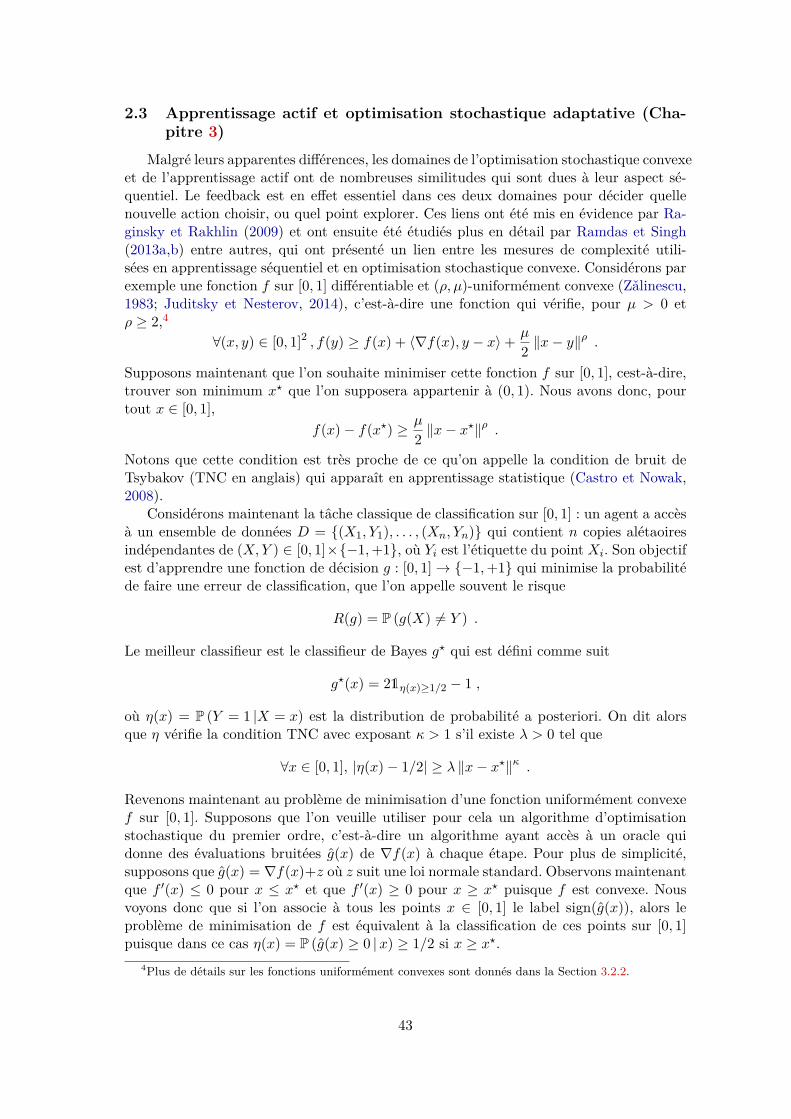
2.3 Apprentissage actif et optimisation stochastique adaptative (Cha-pitre 3)

Malgré leurs apparentes différences, les domaines de l’optimisation stochastique convexeet de l’apprentissage actif ont de nombreuses similitudes qui sont dues à leur aspect sé-quentiel. Le feedback est en effet essentiel dans ces deux domaines pour décider quellenouvelle action choisir, ou quel point explorer. Ces liens ont été mis en évidence par Ra-ginsky et Rakhlin (2009) et ont ensuite été étudiés plus en détail par Ramdas et Singh(2013a,b) entre autres, qui ont présenté un lien entre les mesures de complexité utili-sées en apprentissage séquentiel et en optimisation stochastique convexe. Considérons parexemple une fonction f sur [0, 1] différentiable et (ρ, µ)-uniformément convexe (Zalinescu,1983; Juditsky et Nesterov, 2014), c’est-à-dire une fonction qui vérifie, pour µ > 0 etρ ≥ 2,4

∀(x, y) ∈ [0, 1]2 , f(y) ≥ f(x) + 〈∇f(x), y − x〉+ µ

2 ‖x− y‖ρ .

Supposons maintenant que l’on souhaite minimiser cette fonction f sur [0, 1], cest-à-dire,trouver son minimum x? que l’on supposera appartenir à (0, 1). Nous avons donc, pourtout x ∈ [0, 1],

f(x)− f(x?) ≥ µ

2 ‖x− x?‖ρ .

Notons que cette condition est très proche de ce qu’on appelle la condition de bruit deTsybakov (TNC en anglais) qui apparaît en apprentissage statistique (Castro et Nowak,2008).

Considérons maintenant la tâche classique de classification sur [0, 1] : un agent a accèsà un ensemble de données D = (X1, Y1), . . . , (Xn, Yn) qui contient n copies alétaoiresindépendantes de (X,Y ) ∈ [0, 1]×−1,+1, où Yi est l’étiquette du point Xi. Son objectifest d’apprendre une fonction de décision g : [0, 1]→ −1,+1 qui minimise la probabilitéde faire une erreur de classification, que l’on appelle souvent le risque

R(g) = P (g(X) 6= Y ) .

Le meilleur classifieur est le classifieur de Bayes g? qui est défini comme suit

g?(x) = 21η(x)≥1/2 − 1 ,

où η(x) = P (Y = 1 |X = x) est la distribution de probabilité a posteriori. On dit alorsque η vérifie la condition TNC avec exposant κ > 1 s’il existe λ > 0 tel que

∀x ∈ [0, 1], |η(x)− 1/2| ≥ λ ‖x− x?‖κ .

Revenons maintenant au problème de minimisation d’une fonction uniformément convexef sur [0, 1]. Supposons que l’on veuille utiliser pour cela un algorithme d’optimisationstochastique du premier ordre, c’est-à-dire un algorithme ayant accès à un oracle quidonne des évaluations bruitées g(x) de ∇f(x) à chaque étape. Pour plus de simplicité,supposons que g(x) = ∇f(x)+z où z suit une loi normale standard. Observons maintenantque f ′(x) ≤ 0 pour x ≤ x? et que f ′(x) ≥ 0 pour x ≥ x? puisque f est convexe. Nousvoyons donc que si l’on associe à tous les points x ∈ [0, 1] le label sign(g(x)), alors leproblème de minimisation de f est équivalent à la classification de ces points sur [0, 1]puisque dans ce cas η(x) = P (g(x) ≥ 0 |x) ≥ 1/2 si x ≥ x?.

4Plus de détails sur les fonctions uniformément convexes sont donnés dans la Section 3.2.2.

43

L’analyse de Ramdas et Singh (2013b) montre que pour x ≥ x?,

η(x) = P (g(x) ≥ 0 |x)= P

(f ′(x) + z ≥ 0 |x

)= P (z ≥ 0) + P

(z ∈

[−f ′(x), 0

])≥ 1/2 + λf ′(x) for λ > 0 ,

et que de même pour x ≤ x?,

η(x) ≥ 1/2 + λ|f ′(x)| .

Remarquons maintenant qu’en utilisant l’inégalité de Cauchy-Schwarz, la convexité de fet ensuite son uniforme convexité, nous trouvons que

|∇f(x)||x− x?| ≥ 〈∇f(x), x− x?〉 ≥ f(x)− f(x?) ≥ µ

2 ‖x− x?‖ρ .

Cela montre finalement que

∀x ∈ [0, 1] , |η(x)− 1/2| ≥ λµ

2 ‖x− x?‖ρ−1 ,

ce qui signifie que η vérifie le TNC avec l’exposant κ = ρ− 1 > 1. Cette analyse montreassez simplement les liens qui existent entre le problème de classification active sur [0, 1] etla minimisation d’une fonction uniformément convexe sur [0, 1] en utilisant un algorithmed’optimisation stochastique du premier ordre. Dans (Ramdas et Singh, 2013a) les auteursmettent à profit ce lien pour obtenir un algorithme d’optimisation stochastique convexed’une fonction uniformément convexe en utilisant seulement une information bruitée surles signes du gradient de la fonction. L’algorithme qu’ils proposent utilise une successionde blocs qui contiennent tous une routine d’apprentissage actif.

Un concept important à la fois en apprentissage actif et en optimisation stochastiqueest la quantification de la vitesse de convergence des algorithmes. Cette vitesse dépendgénéralement de la mesure de régularité de la fonction à optimiser, et ainsi dans lesproblèmes détaillés plus haut cette vitesse dépendra soit de l’exposant κ de la conditionTNC, soit de la constante de convexité uniforme ρ. (Ramdas et Singh, 2013b) ont parexemple montré que la vitesse de convergence min-max pour le problème de minimisationstochastique du premier ordre d’une fonction ρ-uniformément convexe et Lipschitz étaitΩ(n−ρ/(2ρ−2)) où n est le nombre d’appels à l’oracle. Nous remarquons d’ailleurs que l’onretrouve la vitesse de convergence Ω(n−1) pour les fonctions fortement convexes (ρ = 2) etla vitesse Ω(n−1/2) pour les fonctions convexes (ρ→∞). Notons en outre que cette vitessede convergence montre bien que la difficulté intrinsèque d’un problème de minimisationest à chercher dans le comportement local de la fonction autour du minimum x? : plus ρest grand, plus la fonction est plate autour du minimum et plus il est donc compliqué dela minimiser.

Cependant lorsque l’on essaye d’optimiser une fonction on ne connaît pas forcémentsa régularité, et plus particulièrement son exposant de convexité uniforme. Cela constituedonc l’une des difficultés de l’optimisation stochastique. Malgré cela plusieurs algorithmesont besoin de connaître ces valeurs pour ajuster leurs propres paramètres. Par exemple,l’algorithme EpochGD (Ramdas et Singh, 2013b) utilise la valeur de ρ, ce qui peut êtreirréaliste en pratique. C’est pour cela que l’on a besoin d’algorithmes “adpatatifs”, quin’ont pas besoin des valeurs des paramètres du problème considéré mais qui peuvent

44

s’y adapter afin d’obtenir les vitesses de convergence souhaitées. En s’inspirant de (Nes-terov, 2009), Juditsky et Nesterov (2014) et Ramdas et Singh (2013a) ont proposé desalgorithmes adaptatifs pour le problème de minimisation stochastique de fonctions uni-formément convexes. Ils ont obtenu la même vitesse de convergence O(n−ρ/(2ρ−2)) queprécédemment, mais cette fois-ci sans utiliser la valeur de ρ. Ces deux algorithmes uti-lisent une succession de blocs dans lequels une valeur approchée de x? est calculée enutilisant soit des techniques de moyennage soit d’apprentissage actif.

Malgré le fait que les méthodes d’optimisation stochastique convexe soient souventdu premier ordre, c’est-à-dire qu’elles utilisent des valeurs bruitées du gradient, il est in-téressant d’étudier d’autres modèles. Par exemple les méthodes d’optimisation convexed’ordre zéro (Bach et Perchet, 2016) visent à optimiser une fonction en utilisant unique-ment des valeurs bruitées du point courant f(xt) + ε. Cela correspond en fait à utiliserun feedback de type “bandit”, c’est-à-dire à connaître seulement la valeur de la fonctionau point choisi pour optimiser f . Généralement, lorsque l’on parle de feedback de typebandit on est plutôt intéressé par minimiser le regret

R(T ) =T∑t=1

f(xt)− f(x?) ,

plutôt que l’erreur f(xT )−f(x?). Minimiser le regret est d’ailleurs plus compliqué puisqueles erreurs faites au début de la phase d’optimisation comptent dans le regret. Ce pro-blème d’optimisation stochastique avec feedback de type bandit a été étudié par (Agarwalet al., 2011) qui ont proposé dans le cas unidimensionnel un algorithme qui utilise troispoints équidistants xl < xc < xr de l’intervalle à explorer, et qui rejette une partie de cetintervalle en fonction des valeurs de f aux trois points. Cet algorithme réalise le regretoptimal O(

√T ). L’idée proposée par Agarwal et al. (2011) est assez semblable à la di-

chotomie, sauf que les auteurs choisissent de rejeter un quart de l’intervalle au lieu de lamoitié dans une dichotomie. Notons en outre qu’il existe des algorithmes d’apprentissageactif ou d’optimisation convexe du premier ordre qui utilisent effectivement des dichoto-mies. C’est par exemple le cas de (Burnashev et Zigangirov, 1974) sur lequel s’appuie letravail de Castro et Nowak (2006).

Il est intéressant de voir que les méthodes d’optimisation stochastiques qui utilisentle gradient ont généralement comme objectif la minimisation de l’erreur sur la fonction,alors qu’il pourrait aussi être pertinent de minimiser le regret, comme dans les problèmesde bandits. Ce sera par exemple le cas dans le problème d’allocation de ressources quenous définirons prochainement.

Nous avons évoqué ici de nombreux algorithmes d’optimisation stochastique qui uti-lisent le gradient. Ainsi, dans la prochaine section nous étudierons le célèbre algorithmede descente de gradient ainsi que sa version stochastique en insistant particulièrement surl’analyse des vitesses de convergence pour le dernier point f(xT )− f(x?).

2.4 Descente de gradient et modèles continus (Chapitre 4)

Considérons maintenant le problème de minimisation d’une fonction f : Rd → Rconvexe et L-lisse5

minx∈Rd

f(x) . (3)

S’il existe de nombreuses méthodes pour résoudre ce problème, les plus courantes sontvraisemblablement les méthodes du premier ordre, c’est-à-dire celles qui utilisent la dé-

5Nous appellerons ici une fonction L-lisse une fonction dérivable dont le gradient est L-Lipschitz.

45

rivée première pour minimiser f . C’est par exemple le cas de l’algorithme de descentede gradient. Ces méthodes sont très en vogue aujourd’hui puisque la taille des donnéesexplose et rend impossible la mise en œuvre de méthodes du second ordre, telles que laméthode de Newton.

L’algorithme de descente de gradient part d’un point x0 ∈ Rd et construit de façonitérative une suite de points approchant x? = arg minx∈Rd f(x) avec la récurrence suivante

xk+1 = xk − η∇f(xk) avec η = 1/L . (4)

Même s’il existe une preuve classique de la convergence de cet algorithme, par exempledans (Bertsekas, 1997), nous voulons proposer ici une analyse différente qui s’appuie surl’équivalent continu de (4). Considérons donc la fonction régulière X : R+ → Rd qui esttelle que X(kη) = xk pour tout k ≥ 0. En utilisant un développement de Taylor à l’ordre1 on trouve

xk+1 − xk = −η∇f(xk)X((k + 1)η)−X(kη) = −η∇f(X(kη))

ηX(kη) + O(η) = −η∇f(X(kη))X(kη) = −∇f(X(kη)) + O(1) ,

ce qui nous incite à considérer l’Équation Différentielle Ordinaire (EDO) suivante

X(t) = −∇f(X(t)), t ≥ 0 . (5)

L’EDO (5), qui est l’équivalent continu du schéma discret (4) peut être facilement étudiéeen analysant la fonction d’énergie suivante, où l’on a noté f? = f(x?),

E(t) , t(f(X(t))− f?) + 12 ‖X(t)− x?‖2 .

En dérivant E et en utilisant la convexité de f on obtient pour tout t ≥ 0,

E ′(t) = f(X(t))− f? + t〈∇f(X(t)), X(t)〉+ 〈X(t)− x?, X(t)〉= f(X(t))− f? − t ‖∇f(X(t))‖2 − 〈∇f(X(t)), X(t)− x?〉≤ −t ‖∇f(X(t))‖2 ≤ 0 .

Ainsi E est décroissante, et pour tout t ≥ 0 on a t(f(X(t)) − f?) ≤ E(t) ≤ E(0) =12 ‖X(0)− x?‖2. Cela nous conduit à la proposition suivante

Proposition 1. Supposons que X : Rd → R vérifie (5). Alors, pour tout t > 0

f(X(t))− f? ≤ 12t ‖X(0)− x?‖2 .

Nous voulons maintenant transposer cette preuve rapide et élégante au cas discret.Nous proposons donc d’introduire la fonction d’énergie discrète suivante

E(k) = kη (f(xk)− f(x?)) + 12 ‖xk − x

?‖2 .

Commençons par un premier lemme.

46

Lemma 1. Si xk et xk+1 sont deux points successifs de la descente de gradient (4) alors

f(xk+1) ≤ f(x?) + 1η〈xk+1 − xk, x? − xk〉 −

12η ‖xk+1 − xk‖2 . (6)

Preuve. On a xk+1 = xk − η∇f(xk) ce qui donne ∇f(xk) = xk − xk+1

η.

Le lemme de descente (Nesterov, 2004, Lemme 1.2.3) et ensuite la convexité de f donnent

f(xk+1) ≤ f(xk) + 〈∇f(xk), xk+1 − xk〉+ L

2 ‖xk+1 − xk‖2

≤ f(x?) + 〈∇f(xk), xk − x?〉+ 〈xk − xk+1

η, xk+1 − xk〉+ 1

2η ‖xk+1 − xk‖2

≤ f(x?) + 1η〈xk+1 − xk, x? − xk〉 −

12η ‖xk+1 − xk‖2 .

Ce deuxième lemme est immédiat et bien connu

Lemma 2. Si xk et xk+1 sont deux points successifs de la descente de gradient (4) alors

f(xk+1) ≤ f(xk)−12η ‖xk+1 − xk‖2 . (7)

Preuve. Le lemme de descente (Nesterov, 2004, Lemme 1.2.3) donne

f(xk+1) ≤ f(xk) + 〈∇f(xk), xk+1 − xk〉+ L

2 ‖xk+1 − xk‖2

≤ f(xk)− 12η ‖xk+1 − xk‖2 .

Nous étudions maintenant E(k). En multipliant l’Équation (6) par 1/(k+1) et l’Équa-tion (7) par k/(k + 1) on obtient

f(xk+1) ≤ k

k + 1f(xk) + 1k + 1f(x?)− 1

2η ‖xk+1 − xk‖2

+ 1k + 1

1η〈xk+1 − xk, x? − xk〉

f(xk+1)− f(x?) ≤ k

k + 1 (f(xk)− f(x?))− 12η ‖xk+1 − xk‖2

+ 1k + 1

1η〈xk+1 − xk, x? − xk〉

(k + 1)η (f(xk+1)− f(x?)) ≤ kη (f(xk)− f(x?))− k + 12 ‖xk+1 − xk‖2 + 〈xk+1 − xk, x? − xk〉 .

Notons alors Ak , (k + 1)η (f(xk+1)− f(x?))− kη (f(xk)− f(x?)). Il vient

Ak ≤ −k + 1

2 ‖xk+1 − xk‖2 + 〈xk+1 − xk, x? − xk〉

≤ k + 12

(−‖xk+1 − x?‖2 − ‖xk − x?‖2 + 2〈xk+1 − x?, xk − x?〉

)+ 〈xk+1 − x?, x? − xk〉+ ‖xk − x?‖2

≤ −k + 12 ‖xk+1 − x?‖2 −

k − 12 ‖xk − x?‖2 + k〈xk+1 − x?, xk − x?〉 .

47

Et ainsi on a

E(k + 1) = (k + 1)η (f(xk+1)− f(x?)) + 12 ‖xk+1 − x?‖2

≤ kη (f(xk)− f(x?))− k

2 ‖xk+1 − x?‖2 −k

2 ‖xk − x?‖2 + 1

2 ‖xk − x?‖2

+ k〈xk+1 − x?, xk − x?〉

≤ E(k)− k

2(‖xk+1 − x?‖2 + ‖xk − x?‖2 − 2〈xk+1 − x?, xk − x?〉

)≤ E(k)− k

2 ‖xk+1 − xk‖2 ≤ E(k) .

Cela montre que (E(k))k≥0 est décroissante et donc que E(k) ≤ E(0) = 12 ‖x0 − x?‖2.

Cela nous permet donc d’établir la proposition suivante qui est l’analogue discret de laProposition 1.Proposition 2. Soit (xk)k∈N vérifiant (4) avec f : Rd → R une fonction convexe etL-lisse. Alors, pour tout k ≥ 1,

f(xk)− f(x?) ≤ L

2k ‖x0 − x?‖2 .

Avec cet exemple simple nous avons montré l’intérêt d’utiliser l’équivalent continud’un problème discret pour intuiter un schéma de preuve pour le problème discret initial.Nous pouvons remarquer que la preuve dans le cas discret est plus complexe que dans lecas continu. Ce sera toujours le cas au long de ce manuscrit. Une des raisons est qu’il estpossible de calculer la dérivée de la fonction d’énergie dans le cas continu alors que c’estimpossible pour une fonction discrète. Un moyen de contourner ce problème est d’utiliserle lemme de descente (Nesterov, 2004, Lemme 1.2.3) qui peut être vu comme une façonde calculer une dérivée discrète, mais avec des termes et des calculs supplémentaires.

À la suite de ces idées, Su et al. (2016) ont récemment proposé un modèle continu pourla célèbre méthode d’accélération de Nesterov (Nesterov, 1983). La méthode d’accélérationde Nesterov est une amélioration de la méthode du moment (Polyak, 1964) qui étaitdéjà elle-même une amélioration de la descente de gradient standard, qui date en faitde Cauchy (1847). L’idée sous-jacente derrière la méthode du moment est de faire diminuerles oscillations en utilisant une fraction des anciennes valeurs des gradients pour calculerle nouveau point. Ce faisant, la récursion utilise donc une moyenne pondérée (avec despoids qui décroissent de façon exponentielle) des précédents gradients et lisse donc lasuite de points en maintenant principalement la direction de descente et en supprimantles oscillations. Cependant, même si la méthode du moment accélère expérimentalement ladescente de gradient, elle n’améliore pas sa vitesse théorique donnée dans la Proposition 2,à la différence de la méthode d’accélération de Nesterov que l’on peut écrire ainsixk+1 = yk − η∇f(yk) avec η ≤ 1/L

yk = xk + k − 1k + 2(xk − xk−1)

. (8)

La méthode de Nesterov utilise aussi l’idée d’un moment, combinée avec un calcul tardifdu gradient, ce qui conduit à une meilleure vitesse de convergence :Théorème 1. Soit f une fonction convexe et L-lisse. Alors la méthode d’accélération deNesterov vérifie pour tout k ≥ 1

f(xk)− f(x?) ≤ 2L ‖x0 − x?‖2

k2 .

48

Cette vitesse de convergence qui améliore celle de la Proposition 2 atteint la borneinférieure de (Nesterov, 2004, Théorème 2.1.7), mais la preuve n’est pas du tout intui-tive ni les idées aboutissant au schéma (8). Le schéma continu introduit par Su et al.(2016) apporte en revanche davantage de compréhension au phénomène d’accélération enproposant d’étudier l’équation différentielle du deuxième ordre

X(t) + 3tX(t) +∇f(X(t)) = 0, t ≥ 0 .

Les auteurs prouvent la vitesse de convergence suivante pour le modèle continu

pour tout t > 0, f(X(t))− f? ≤ 2 ‖X(0)− x?‖2

t2,

à nouveau en introduisant une énergie appropriée, et dans ce cas E(t) = t2 (f(X(t))− f?)+2‖X(t) + tX(t)/2− x?‖2 qui est décroissante.

Après avoir effectué cette analyse de l’algorithme de descente de gradient ainsi que decertaines de ses variantes, il est naturel de s’intéresser au cas stochastique. La descente degradient est en effet très utilisée en apprentissage automatique, et plus particulièrementen apprentissage profond où des algorithmes proches de la descente de gradient serventà minimiser les fonctions de perte de réseaux de neurones, et à apprendre les poids deces neurones. En apprentissage profond on est généralement intéressé par minimiser desfonctions f qui ont la forme suivante

f(x) = 1N

N∑i=1

fi(x) , (9)

où fi est associée à la i-ème observation des données d’entraînement (qui sont en nombreN , généralement très grand). C’est pour cela que calculer le gradient de f est très coûteuxpuisque que cela nécessite de calculer les N gradients ∇fi. Afin d’accélérer la phased’entraînement on choisit donc généralement d’approximer le gradient de f par ∇fi où iest choisi uniformément au hasard entre 1 et N . On peut aussi faire un compromis entrece choix et la descente de gradient classique en utilisant un “mini lot”, c’est-à-dire unpetit ensemble de points de 1, . . . , N pour calculer le gradient :

∇f(x) ≈ 1M

M∑i=1∇fσ(i)(x) ,

où σ est une permutation de 1, . . . , N et M est la taille du mini lot. Ces deux choixpermettent de calculer une valeur approchée g(x) du vrai gradient ∇f(x) qui en constitueun estimateur non biaisé (E [g(x)] = ∇f(x)) puisque les points utilisés pour calculer cesapproximations sont choisis uniformément au hasard. En utilisant ces approximationsstochastiques de ∇f(x) à la place de la valeur exacte du gradient dans l’algorithme dedescente de gradient on obtient l’algorithme de “Descente de Gradient Stochastique”(SGD en anglais), qui a une formulation plus générale que celle obtenue ci-dessus. Eneffet l’algorithme SGD apporte une solution au problème de minimisation (3) en utilisantdes valeurs bruitées de ∇f et ne se restreint pas aux fonctions de la forme (9).

Obtenir des vitesses de convergence pour SGD est bien plus complexe que pour ladescente de gradient, à cause des incertitudes dues à son côté stochastique. Dans le casde SGD le but est en réalité de borner E [f(xk)] − f? parce que la suite (xk)k≥0 estmaintenant aléatoire. Dans le cas où f est fortement convexe les résultats de convergence

49

sont bien connus (Nemirovski et al., 2009; Bach et Moulines, 2011) mais dans le cas où fest simplement convexe ils ne sont pas aussi communs. En effet la majorité des résultatsde convergence connus dans le cas convexe sont obtenus dans le cadre du moyennage dePolyak-Ruppert (Polyak et Juditsky, 1992; Ruppert, 1988) où au lieu de considérer ledernier point xN on considère la valeur moyenne xN

xN = 1N

N∑k=1

xk .

Il est plus facile d’obtenir des vitesses de convergence dans le cas du moyennage (Nemi-rovski et al., 2009) que d’obtenir des vitesses non asymptotiques pour le dernier point.En effet ces dernières impliquent directement avec l’inégalité de Jensen des vitesses deconvergence dans le cas du moyennage. Il est d’ailleurs intéressant de remarquer à cepropos que les algorithmes présentés dans la Section 2.3 portent sur la version moyennéedes itérés et non sur le dernier point. À notre connaissance il n’existe pas de résultat deconvergence général dans le cas convexe et lisse pour SGD. L’un des seuls résultas donton dispose pour le dernier itéré est en effet dû à Shamir et Zhang (2013) qui font l’hypo-thèse que les points restent dans un compact, ce qui est évidemment une hypothèse forte.Finalement Bach et Moulines (2011) conjecturent que la vitesse de convergence optimalepour SGD dans le cas convexe est O(k−1/3), ce que nous contredisons dans le Chapitre 4.

3 Plan du manuscript et contributionsCette thèse sera divisée en quatre chapitres, qui correspondent chacun à l’un des

problèmes que nous avons étudiés. Chacun de ces chapitres a donné lieu à une publicationou à une pré-publication. Nous avons décidé de regrouper les trois premiers chapitresen une première partie qui porte sur l’apprentissage séquentiel, tandis que le dernierchapitre fera l’objet d’une seconde partie assez différente sur l’optimisation stochastique.Le Chapitre 3 peut être vu comme un lien entre les deux parties.

Nous présentons maintenant un résumé de nos contributions principales ainsi que desrésultats obtenus dans les prochains chapitres de cette thèse. L’objectif des sections quisuivent est de résumer ces résultats, et non de donner les énoncés exacts et exhaustifsdes différents hypothèses et théorèmes. Nous nous sommes efforcés de rendre cette partiefacilement lisible et nous invitons le lecteur à se diriger vers les chapitres correspondantspour obtenir tous les détails souhaités.

3.1 Partie I Chapitre 1

Dans ce chapitre nous étudions le problème de bandits stochastiques contextuels avecrégularisation en adoptant un point de vue non paramétrique. Plus précisément, commeexpliqué dans la Section 2.1 nous considérons un ensemble de K ∈ N∗ bras à qui l’onassocie les fonctions de récompense µk : X → R qui correspondent aux espérances condi-tionnelles des récompenses de chaque bras sachant le contexte, qui est tiré uniformémentau hasard parmi un ensemble X = [0, 1]d. Chacune de ces fonctions est supposée β-Hölder.En notant p : X → ∆K la mesure d’occupation de chaque bras notre objectif est alors deminimiser la fonction de perte

L(p) =∫X〈µ(x), p(x)〉+ λ(x)ρ(p(x)) dx ,

50

où ρ : ∆K → R est une fonction de régularisation convexe (typiquement l’entropie) etλ : X → R est une fonction modulant la régularisation. Nous allons supposer que ces deuxfonctions sont connues par l’agent et sont différentiables.

Nous notons p? la fonction des proportions optimales

p? = arg infp∈f :X→∆K

L(p) ,

et nous développons dans le Chapitre 1 un algorithme qui renvoie au bout de T itérationsune fonction de proportions pT qui minimise le regret

R(T ) = E [L(pT )]− L(p?) .

Puisque pT est en fait le vecteur des fréquences empiriques de chaque bras, R(T ) doit êtrevu comme un regret cumulé. Nous analysons ensuite l’algorithme que nous avons proposéafin d’obtenir des bornes supérieures sur le regret avec différentes hypothèses. Notre al-gorithme utilise une partition de l’espace des contextes et résout de façon indépendanteun problème d’optimisation convexe sur chacun des sous-ensembles de la partition.

Nous commençons par établir des vitesses de convergence dans le cas où λ est unefonction constante et avec des hypothèses faibles sur les autres paramètres du problème.Nous appellerons “vitesses lentes” les vitesses plus lentes queO(T−1/2) (et réciproquement“vitesses rapides” les bornes de convergence plus rapides que O(T−1/2)).

Théorème 2. Si λ est constante et que ρ est une fonction convexe et lisse alors nousobtenons la vitesse de convergence lente suivante pour le regret, pour tout T ≥ 1,

R(T ) ≤ O

( T

log(T )

)− β2β+d

.

Si nous supposons en plus que ρ est fortement convexe et que le minimum de lafonction de perte sur chaque sous-ensemble de la partition est atteint loin des bords de∆K alors nous obtenons des vitesses plus rapides

Théorème 3. Si λ est constante et que ρ est une fonction fortement convexe et lisse, etsi L atteint son minimum loin6 de ∂∆K , alors nous obtenons la vitesse de convergencerapide suivante pour le regret, pour tout T ≥ 1,

R(T ) ≤ O

( T

log(T )2

)− 2β2β+d

.

Cette vitesse rapide cache cependant un facteur multiplicatif qui fait intervenir 1/λ et1/η (où η est la distance de l’optimum aux bords de ∆K) et qui peut être arbitrairementgrand. Nous nous intéressons donc maintenant au cas où λ est une fonction du contexte,c’est-à-dire que l’agent peut moduler le poids de la régularisation en fonction du contexte.Dans ce cas la distance de l’optimum au bord ∂∆K dépendra aussi de la valeur du contexteet nous définissons donc la fonction η comme suit

η(x) := dist(p?(x), ∂∆K) ,

où p?(x) ∈ ∆K est le point où (p 7→ 〈µ(x), p〉 + λ(x)ρ(p)) atteint son minimum. Afinde pouvoir supprimer toute dépendence en λ et η dans notre borne du regret, tout en

6Voir Section 1.4.2 pour un énoncé plus précis.

51

obtenant des vitesses plus rapides que celles du Théorème 2 nous devons faire une hypo-thèse supplémentaire qui va empêcher λ et η de prendre trop souvent des petites valeurs(qui sont la raison d’un facteur multiplicatif trop important dans le Théorème 3). Ceciest classique en estimation non paramétrique et nous faisons donc l’hypothèse suivante,autrement appelée “condition de marge”

Hypothèse 1. Il existe δ1 > 0, δ2 > 0, α > 0 et Cm > 0 tels que

∀δ ∈ (0, δ1], PX(λ(x) < δ) ≤ Cmδ6α et ∀δ ∈ (0, δ2], PX(η(x) < δ) ≤ Cmδ6α .

Cette condition dépend d’un paramètre de marge α qui contrôle la difficulté du pro-blème et qui permet d’obtenir des vitesses de convergence intermédiaires qui interpolentparfaitement entre les vitesses lentes et les vitesses rapides, sans avoir de dépendance enη ou en λ.

Théorème 4. Si ρ est une fonction convexe, alors avec une condition de marge de pa-ramètre α ∈ (0, 1) nous obtenons la vitesse de convergence suivante pour le regret, pourtout T ≥ 1,

R(T ) = O

( T

log2(T )

)− β2β+d (1+α)

.

Nous pouvons nous demander si les résultats de convergence obtenus dans les troisthéorèmes présentés ci-dessus sont optimaux ou pas. Remarquons déjà que ces vitessesde convergence sont classiques en estimation non paramétrique (Tsybakov, 2008). Quiplus est, nous prouvons aussi à la fin du chapitre une borne inférieure pour notre pro-blème, qui montre que la vitesse de convergence du Théorème 3 est optimale aux termeslogarithmiques près.

Théorème 5. Pour tout algorithme de bandits qui renvoie pT , avec ρ fortement convexeet µ β-Hölder, il existe une constante universelle C telle que

infp

supρ,µ

E[L(pT )]− L(p?)

≥ C T−

2β2β+d .

Nous terminons ce chapitre avec des expériences numériques sur des données synthé-tiques qui illustrent de façon empirique nos résultats de convergence.

3.2 Partie I Chapitre 2

Dans ce chapitre nous cherchons à estimer de façon active la matrice de design pour leproblème de régression linéaire détaillé à la Section 2.2. Le but ici est d’obtenir la meilleureestimation possible du paramètre β? de la régression linéaire, c’est-à-dire de construireun estimateur β à l’aide de T échantillons qui minimise la norme `2 E[‖β? − β‖2]. Enintroduisant la matrice suivante

Ω(p) =K∑k=1

(pk/σ2k )XkX

>k ,

nous voyons que notre problème correspond en réalité à minimiser la trace de l’inverse dela matrice Ω(p) (qui est la matrice de covariance du problème), puisque

E[‖β − β?‖2

]= 1TTr(Ω(p)−1) .

52

Ainsi notre problème est équivalent à la planification en ligne et optimale d’expériencesavec le critère A. Plus précisément, introduisons la fonction de perte L(p) = Tr(Ω(p)−1)qui est strictement convexe et qui admet donc un minimum p?. Notre objectif se reformuledonc en la minimisation du regret de notre algorithme, c’est-à-dire que nous cherchons àminimiser l’écart entre la perte de l’algorithme et la plus petite perte réalisable

R(T ) = E[‖β − β?‖2

]−min

algoE[‖β(algo) − β?‖2

]= 1T

(E [L(pT )]− L(p?)) .

De la même façon qu’à la Section 3.1 notons que R(T ) n’est pas un regret simple maisbien un regret cumulé.

Dans le Chapitre 2 nous construisons un algorithme d’apprentissage actif pour ré-soudre le problème de planification en ligne et optimale d’expériences en nous appuyantsur le travail de Berthet et Perchet (2017). Remarquons que lorsque K < d la matriceΩ(p) est dégénérée, ce qui conduit à un regret linéaire, à moins de restreindre l’analyse ausous-espace induit par les covariables. C’est ce que nous ferons par la suite, ce qui permetdonc de considérer maintenant que K ≥ d.

Après avoir obtenu un résultat de concentration sur les variances de variables aléa-toires sous-gaussiennes nous analysons notre algorithme, en distinguant deux cas. Dans lepremier cas le nombre de covariables K est égal à la dimension de l’espace d. Nous savonsdonc que tous ces points doivent être tirés un nombre non nul de fois, mais le contrôle dela quantité de tirages est crucial. Nous utilisons donc au début de l’algorithme une phasede pré-échantillonnage de chaque bras qui force la fonction de perte à être localement lisseet qui nous permet d’obtenir des vitesses de convergence rapides.

Théorème 6. Dans le cas où K = d nous obtenons la vitesse de convergence rapidesuivante, pour tout T ≥ 1,

R(T ) = O(

log2(T )T 2

).

Il est important de mentionner que cette vitesse rapide n’est pas facile à obtenir. Eneffet, à la Section 2.3 nous présentons un algorithme naïf qui s’appuie sur des techniquessimilaires à celles utilisées par UCB, et qui n’atteint qu’un regret en O(T−3/2).

Dans le second cas où K > d le problème est bien plus difficile. En effet de nombreusessituations différentes peuvent avoir lieu et le point d’optimum p? peut être atteint soit enn’échantillonnant pas certains points, soit en les tirant tous. Trouver la stratégie optimaleest donc un problème difficile, ce qui explique la vitesse de convergence plus faible quenous obtenons dans ce cas

Théorème 7. Dans le cas où K > d nous obtenons la vitesse de convergence suivantepour le regret, pour tout T ≥ 1

R(T ) = O( log(T )T 5/4

).

Cette borne supérieure n’est pas optimale et nous prouvons d’ailleurs la borne infé-rieure suivante dans le cas où K > d

Théorème 8. Pour tout algorithme sur notre problème il existe un ensemble de para-mètres tels que R(T ) & T−3/2.

Les expériences numériques que nous réalisons à la fin du Chapitre 2 illustrent bienle fait que le cas K > d est bien plus complexe que le cas K = d et que la vitesse deconvergence optimale se trouve certainement entre T−5/4 et T−3/2.

53

3.3 Partie I Chapitre 3

Dans ce chapitre nous étudions un problème à la frontière entre l’apprentissage séquen-tiel et l’optimisation convexe stochastique, qui est un problème d’allocation de ressourcesque nous formulons de la façon suivante. Supposons qu’un agent a accès à un ensemblede K différentes ressources auxquelles il peut allouer un montant xk, qui génère une ré-compense fk(xk). À chaque pas de temps l’agent ne peut qu’allouer un budget total fini,c’est-à-dire que ∑K

k=1 xk = 1. Ainsi l’agent reçoit à chaque pas de temps t ∈ 1, . . . , T larécompense

F (x(t)) =K∑k=1

fk(x(t)k ) avec x(t) = (x(t)

1 , . . . , x(t)K ) ∈ ∆K ,

qui doit être maximisée. En notant x? ∈ ∆K l’allocation optimale qui maximise F , l’ob-jectif de l’agent est équivalent à la minimisation du regret cumulé

R(T ) = F (x?)− 1T

T∑t=1

K∑k=1

fk(x(t)k ) = max

x∈∆KF (x)− 1

T

T∑t=1

F (x(t)) .

Les problèmes d’allocation de ressources ont été étudiés pendant des siècles dans de nom-breux domaines d’application et nous faisons maintenant une hypothèse classique quiremonte à Smith (1776) et qui porte le nom d’hypothèse des “rendements décroissants”,et qui peut être modélisée par des fonctions de récompense concaves. Dans ce chapitrenous supposerons que l’agent a aussi accès à chaque pas de temps à une valeur bruitéede ∇F (x(t)) pour réaliser la minimisation du regret, ce qui place l’agent en compétitionavec d’autres algorithmes d’optimisation stochastique du premier ordre.

Afin de mesurer la complexité du problème que nous étudions nous faisons une hy-pothèse supplémentaire qui s’appuie sur l’inégalité de Łojasiewicz (Łojasiewicz, 1965),qui correspond à une forme plus faible de la convexité uniforme. L’hypothèse précise surlaquelle nous travaillons est expliquée en détails à la Section 3.2.3 mais nous en énonçonsun cas particulier ici par simplicité.

Hypothèse 2. Pour tout k ∈ 1, · · · ,K, fk est ρ-uniformément concave.

Avec cette hypothèse nous dirons que nous vérifions “inductivement” l’inégalité deŁojasiewicz avec le paramètre β = ρ

ρ−1 , comme le montre la Proposition 3.5.L’exposant dans l’inégalité de Łojasiewicz étant supposé inconnu, l’objectif du Cha-

pitre 3 est de construire un algorithme adaptatif à cet exposant et qui minimise le regret.Si nous revenons à la discussion de la Section 2.3 nous cherchons ici à minimiser le re-gret, ce qui est plus compliqué que de minimiser l’erreur sur la fonction. Ce faisant, cetobjectif nous empêche d’utiliser les algorithmes proposés par Juditsky et Nesterov (2014)ou Ramdas et Singh (2013a) qui obtiennent un regret linéaire.

Nous construisons un algorithme dont le concept central est la dichotomie. Nous enprésentons ici un aperçu dans le cas de K = 2 ressources, où l’on a donc F (x) = f1(x1) +f2(x2) = f1(x1) + f2(1− x1) , f1(x) + f2(1− x), qui peut être vue comme une fonctiondéfinie sur [0, 1]. L’idée de l’algorithme est d’évaluer chaque point d’échantillonnage x unnombre suffisant de fois pour obtenir avec grande probabilité le signe de ∇F (x), qui nousdira si x? est à droite ou à gauche du point courant x. Notre algorithme consiste donc enune dichotomie qui supprime la moitié de l’intervalle de recherche à chaque phase. Puisqueles points qui sont loin de x? seront peu échantillonnés (car le signe du gradient à ces pointsest facile à déterminer) notre algorithme a un regret sous-linéaire. Il est facile de montrer

54

que son regret est même O(T−1) dans le cas fortement convexe, ce qui coïncide avec lavitesse classique d’optimisation stochastique pour des fonctions fortement convexes. Dansle cas général nous obtenons la vitesse de convergence suivante en imbricant plusieursdichotomies les unes dans les autres.

Théorème 9. Si le problème vérifie inductivement l’inégalité de Łojasiewicz avec β ≥ 1alors nous obtenons la borne suivante sur le regret, après T ≥ 1 échantillons

dans le cas β > 2, E[R(T )] ≤ O(K

log(T )log2(K)

T

);

dans le cas β ≤ 2, E[R(T )] ≤ O

K (log(T )log2(K)+1

T

)β/2 .

Notons que sous l’Hypothèse 2, β = ρ/(ρ − 1) ≤ 2 et nous obtenons donc une bornesur le regret en T−ρ/(2ρ−2), ce qui est exactement la vitesse obtenue par Ramdas etSingh (2013a,b) et Juditsky et Nesterov (2014), mais cette fois pour le regret et nonpour la minimisation de la fonction. Comme dans les chapitres précédents nous analysonsl’optimalité de la borne supérieure du théorème précédent en prouvant la borne inférieuresuivante dans le cas où β ∈ [1, 2]

Théorème 10. Pour tout algorithme il existe une paire de fonctions concaves et crois-santes f1 et f2 telles que

E [R(T )] ≥ cβT−β2 ,

où cβ > 0 est une constante indépendante de T .

Ce résultat montre que notre borne supérieure est optimale aux facteurs logarith-miques près. Nous finissons le chapitre en illustrant nos résultats théoriques par des ex-périences numériques réalisées sur des données synthétiques.

Par ailleurs nous mettons aussi en évidence dans ce chapitre que notre problème géné-ralise le problème des bandits multi-bras, en s’intéressant au cas des ressources linéaires.Nous retrouvons ainsi à la Section 3.3.5 la borne classique en log(T )/(T∆) des banditsmulti-bras.

3.4 Partie II Chapitre 4

Dans ce chapitre nous analysons l’algorithme de Descente de Gradient Stochastique(SGD) que nous avons évoqué à la Section 2.4. Soit f : Rd → R la fonction à minimiser,que l’on suppose continûment dérivable et lisse. Nous faisons l’hypothèse que nous n’avonspas accès ∇f(x) mais plutôt à des estimations non biaisées H(x, z) où z est une réalisationd’une variable aléatoire Z sur Z de densité µZ qui vérifie

∀x ∈ Rd,∫

ZH(x, z)dµZ(z) = ∇f(x) .

Nous définissons alors SGD comme suit

Xn+1 = Xn − γ(n+ 1)−αH(Xn, Zn+1) , (10)

où γ > 0 est le pas initial, α ∈ [0, 1] est un paramètre permettant d’utiliser des pas dé-croissants et (Zn)n∈N est une suite de variables aléatoires indépendantes distribuées selon

55

µZ. Comme expliqué dans la Section 2.4 nous étudions SGD en analysant son pendantcontinu qui vérifie l’Équation Différentielle Stochastique (EDS) suivante

dXt = −(γα + t)−α∇f(Xt)dt+ γ1/2α Σ(Xt)1/2dBt , (11)

où γα = γ1/(1−α), Σ(x) = µZ(H(x, ·) − ∇f(x)H(x, ·) − ∇f(x)>) et (Bt)t≥0 est unmouvement brownien d-dimensionnel.

Une de nos contributions dans le Chapitre 4 est de proposer une nouvelle méthode pourobtenir les vitesses de convergence de SGD, qui utilise l’analyse de l’EDS correspondante.Cette méthode a l’avantage d’être plus simple que les preuves existantes, et nous mettonscela en évidence avec l’exemple des fonctions fortement convexes. Notre méthode consisteà trouver une fonction d’énergie appropriée qui va donner les vitesses de convergence dansle cas continu, et ensuite à adapter la preuve au cas discret en utilisant des techniquessimilaires, le cas continu servant donc à obtenir l’intuition de la preuve. Nous prouvonspar exemple le résultat suivant dans le cas fortement convexe.

Théorème 11. Si f est une fonction lisse et fortement convexe, le schéma SGD (10) quiutilise des pas décroissants de paramètre α ∈ (0, 1] a la vitesse de convergence suivantepour tout N ≥ 1,

E[‖XN − x?‖2

]≤ CN−α .

Malgré le fait que ce résultat est déjà connu, la preuve que nous proposons est beaucoupplus simple que celle de Bach et Moulines (2011). Pour faire l’analyse du schéma continunous utilisons le lemme de Dynkin (qui consiste essentiellement à prendre l’espérancedans le lemme d’Itô, voir Lemme 4.13) afin de calculer la dérivée de l’énergie. Dans le casdiscret nous remplaçons le lemme de Dynkin par le lemme de descente (Nesterov, 2004,Lemme 1.2.3) qui est un équivalent approché discret du lemme de Dynkin, mais qui ne faitpas intervenir la dérivée seconde, ce qui va conduire à des preuves légèrement différentes.

La contribution principale du Chapitre 4 est une analyse exhaustive de SGD dansle cas convexe pour la convergence de la fonction au dernier itéré. Nous considérons eneffet la situation où f est convexe et lisse sans faire d’hypothèse de compacité. Nousprouvons alors les deux résultats suivants grâce à des arguments assez similaires. Lepremier théorème donne la vitesse de convergence de l’EDS (11).

Théorème 12. Si f est une fonction lisse et convexe, alors il existe C ≥ 0 tel que lasuite (Xt)t≥0 définie par l’EDS (11) avec paramètre α ∈ (0, 1) vérifie pour tout T ≥ 1,

E [f(XT )]− f? ≤ C(1 + log(T ))2/Tα∧(1−α) .

Nous prouvons un deuxième résultat similaire dans le cas discret. La preuve est unpeu plus complexe du fait des différences entre le lemme de Dynkin et le lemme dedescente, mais nous obtenons néanmoins le résultat suivant dont la ressemblance avec leThéorème 12 illustre bien les liens entre les modèles discret et continu.

Théorème 13. Si f est une fonction lisse et convexe alors il existe C ≥ 0 tel que la suitede SGD définie par (10) pour α ∈ (0, 1) vérifie pour tout N ≥ 1,

E [f(XN )]− f? ≤ C(1 + log(N + 1))2/(N + 1)α∧(1−α) .

Ce dernier résultat vient contredire la conjecture de Bach et Moulines (2011) quisupposaient que la vitesse optimale de convergence pour le dernier itéré dans SGD étaitN−1/3.

56

Pour finir nous nous intéressons au cas où f n’est plus convexe. Nous considéronspour cela une généralisation du cas “faiblement quasi-convexe” (Hardt et al., 2018) ensupposant qu’il existe r1 ∈ (0, 2), r2 ≥ 0, τ > 0 tels que pour tout x ∈ Rd,

f(x)− f(x?) ≤ ‖∇f(x)‖r1 ‖x− x?‖r2 /τ .

Notons en outre que cette condition englobe le cas où f vérifie l’inégalité de Łojasie-wicz mentionnée à la Section 3.3 qui peut être définie de la façon suivante pour β ∈ (0, 2)et c > 0,

∀x ∈ Rd, f(x)− f(x?) ≤ c ‖∇f(x)‖β ,

et qui a été abondamment utilisée en optimisation.Sous ces hypothèses nous sommes à nouveau en mesure d’obtenir des vitesses de

convergence, à la fois pour l’EDS (11) et pour le schéma discret de SGD (10). Ces ré-sultats qui sont rigoureusement établis à la Section 4.3.4 généralisent et améliorent lesbornes précédemment obtenues dans le cas faiblement quasi-convexe par Orvieto et Lucchi(2019).

3.5 Liste des publications

Cette thèse a donné lieu aux publications suivantes :

• (Fontaine et al., 2019a) Regularized Contextual Bandits, Xavier Fontaine,Quentin Berthet and Vianney Perchet, International Conference on Artifical In-telligence and Statistics (AISTATS), 2019

• (Fontaine et al., 2019b) Online A-Optimal Design and Active Linear Regres-sion, Xavier Fontaine, Pierre Perrault, Michal Valko and Vianney Perchet, soumis

• (Fontaine et al., 2020b) An adaptive stochastic optimization algorithm forresource allocation, Xavier Fontaine, Shie Mannor and Vianney Perchet, Inter-national Conference on Algorithmic Learning Theory (ALT), 2020

• (Fontaine et al., 2020a) Convergence rates and approximation results forSGD and its continuous-time counterpart, Xavier Fontaine, Valentin De Bor-toli and Alain Durmus, soumis.

L’auteur a aussi participé à la publication suivante, qui n’est pas traitée dans cettethèse :

• (De Bortoli et al., 2020)Quantitative Propagation of Chaos for SGD in WideNeural Networks, Valentin de Bortoli, Alain Durmus, Xavier Fontaine and UmutŞimşekli, Advances in Neural Information Processing Systems, 2020.

Dans la suite de cette thèse nous avons fait le choix de déplacer les preuves les pluslongues dans les appendices de fin de chapitre pour des raisons de lisibilité.

57

58

Part I

Sequential learning

59

1 Regularized contextual bandits

In this chapter we consider the stochastic contextual bandit problem with additionalregularization. The motivation comes from problems where the policy of the agentmust be close to some baseline policy known to perform well on the task. To tackle thisproblem we use a nonparametric model and propose an algorithm splitting the contextspace into bins, solving simultaneously — and independently — regularized multi-armed bandit instances on each bin. We derive slow and fast rates of convergence,depending on the unknown complexity of the problem. We also consider a newrelevant margin condition to get problem-independent convergence rates, yieldingintermediate rates interpolating between the aforementioned slow and fast rates1.

1.1 Introduction and related workIn sequential optimization problems, an agent takes successive decisions in order to min-imize an unknown loss function. An important class of such problems, nowadays knownas bandit problems, has been mathematically formalized by Robbins in his seminal pa-per (Robbins, 1952). In the so-called stochastic multi-armed bandit problem, an agentchooses to sample (or “pull”) among K arms returning random rewards. Only the re-wards of the selected arms are revealed to the agent who does not get any additionalfeedback. Bandit problems naturally model the exploration/exploitation trade-offs whicharise in sequential decision making under uncertainty. Various general algorithms havebeen proposed to solve this problem, following the work of Lai and Robbins (1985) whoobtain a logarithmic regret for their sample-mean based policy. Further bounds have beenobtained by Agrawal (1995) and Auer et al. (2002) who developed different versions ofthe well-known UCB algorithm.

The setting of classical stochastic multi-armed bandits is unfortunately too restrictivefor real-world applications. The choice of the agent can and should be influenced by addi-tional information (referred to as “context” or “covariate”) revealed by the environment.It encodes features having an impact on the arms’ rewards. For instance, in online ad-vertising, the expected Click-Through-Rate depends on the identity, the profile and thebrowsing history of the customer. These problems of bandits with covariates have beeninitially introduced by Woodroofe (1979) and have attracted much attention since Wang

1This chapter is joint work with Quentin Berthet and Vianney Perchet. It has led to the followingpublication:(Fontaine et al., 2019a) Regularized Contextual Bandits, Xavier Fontaine, Quentin Berthet andVianney Perchet, International Conference on Artificial Intelligence and Statistics (AISTATS), 2019.

61

et al. (2005); Goldenshluger et al. (2009). This particular class of bandits problems is nowknown under the name of contextual bandits following the work of Langford and Zhang(2008).

Contextual bandits have been extensively studied in the last decades and several im-provements upon multi-armed bandits algorithms have been applied to contextual ban-dits, including Thompson sampling (Agrawal and Goyal, 2013), Explore-Then-Commitstrategies (Perchet and Rigollet, 2013), and policy elimination (Dudik et al., 2011). Theyare quite intricate to study as they borrow aspects from both supervised learning andreinforcement learning. Indeed they use features to encode the context variables, as in su-pervised learning but also require an exploration phase to discover all the possible choices.Applications of contextual bandits are numerous, ranging from online advertising (Tanget al., 2013), to news articles recommendation (Li et al., 2010) or decision-making in thehealth and medicine sectors (Tewari and Murphy, 2017; Bastani and Bayati, 2015).

Among the general class of stochastic multi-armed bandits, different settings can bestudied. One natural hypothesis that can be made is to consider that the arms’ rewardsare regular functions of the context i.e., that two close context values have similar expectedrewards. This setting has been studied in (Srinivas et al., 2010), (Perchet and Rigollet,2013) and (Slivkins, 2014). A possible approach to this problem is to take inspirationfrom the regressograms used in nonparametric estimation (Tsybakov, 2008) and to dividethe context space into several bins. This technique also used in online learning (Hazanand Megiddo, 2007) leads to the concept of UCBograms (Rigollet and Zeevi, 2010) inbandits.

We introduce regularization to the problem of stochastic multi-armed bandits. Itis a widely-used technique in machine learning to avoid overfitting or to solve ill-posedproblems. Here the regularization forces the solution of the contextual bandits problemto be close to an existing known policy. As an example of motivation, an online-advertiseror any decision-maker may wish not to diverge too much from a handcrafted policy thatis known to perform well. This has already motivated previous work such as ConservativeBandits (Wu et al., 2016), where an additional arm corresponding to the handcraftedpolicy is added. By adding regularization, the agent can be sure to end up close to thechosen policy. Within this setting the form of the objective function is not a classicalbandit loss anymore, but contains a regularization term on the global policy. We falltherefore in the more general setting of online optimization and borrow tools from this fieldto build and analyze an algorithm on contextual multi-armed bandits. As a substituteof the UCB algorithm we use the recently introduced Upper Confidence-Frank Wolfealgorithm (Berthet and Perchet, 2017).

Our main contribution consists in an algorithm with proven slow or fast rates ofconvergence, depending on the unknown complexity of the problem at hand. These ratesare better than the ones obtained for classical nonparametric contextual bandits. Basedon nonparametric statistics we obtain parameter-independent intermediate convergencerates when the regularization function depends on the context value.

The remainder of this chapter is organized as follows. We present the setting andproblem in Section 1.2. Our algorithm is described in Section 1.3. Sections 1.4 and 1.5 aredevoted to deriving the convergence rates. Lower bounds are detailed in Section 1.6 andexperiments are presented in Section 1.7. Section 1.8 concludes the chapter. Postponedproofs are put in Appendix 1.A.

62

1.2 Problem setting and definitions

1.2.1 Problem description

We consider a stochastic contextual bandit problem with K ∈ N∗ arms and time horizonT . It is defined as follows. At each time t ∈ 1, . . . , T, Nature draws a context variableXt ∈ X = [0, 1]d uniformly at random. This context is revealed to an agent who choosesan arm πt amongst the K arms. Only the loss Y (πt)

t ∈ [0, 1] is revealed to the agent.For each arm k ∈ 1, . . . ,K we note µk(X) , E(Y (k)|X) the conditional expectation

of the arm’s loss given the context. We impose classical regularity assumptions on thefunctions µk borrowed from nonparametric estimation (Tsybakov, 2008). Namely wesuppose that the functions µk are (β, Lβ)-Hölder, with β ∈ (0, 1]. We note Hβ,Lβ thisclass of functions.

A1.1 (β-Hölder). There exists β ∈ (0, 1] and Lβ > 0 such that for all k ∈ [K]2, µk isβ-Hölder i.e.,

∀x, y ∈ X , |µk(x)− µk(y)| ≤ Lβ ‖x− y‖β .

Unless explicitly specified we will only consider the classical euclidean norm on Rdin this chapter. We denote by p : X → ∆K the proportion function of each arm (alsocalled occupation measure), where ∆K is the unit simplex of RK . In classical stochasticcontextual bandits the goal of the agent is to minimize the following loss function

L(p) =∫X〈µ(x), p(x)〉dx .

We add a regularization term representing the constraint on the optimal proportion func-tion p?. For example we may want to encourage p? to be close to a chosen proportionfunction q, or to be far from ∂∆K . In order to do that we consider a convex regularizationfunction ρ : ∆K × X → R and a regularization parameter λ : X → R. Both ρ and λ areknown and given to the agent, while the µk functions are unknown and must be learned.We want to minimize the loss function

L(p) =∫X〈µ(x), p(x)〉+ λ(x)ρ(p(x), x) dx . (1.1)

This is the most general form of the loss function. We study first the case where theregularization does not depend on the context (i.e., when λ is a constant and when ρ isonly a function of p).

The function λ modulates the weight of the regularization and is chosen to be regularenough. More precisely we make the following assumption on the regularization term.

A1.2. λ is a C∞ non-negative function and ρ is a C1 convex function.

We will see later the convexity of ρ is not enough and that we actually need strongconvexity.

Definition 1.1. We say that ρ is a C1 ζ-strongly convex function with ζ > 0 if ρ iscontinuously differentiable and if

∀ (p, q) ∈ (∆K)2, ρ(q) ≥ ρ(p) + 〈∇ρ(p), q − p〉+ ζ

2 ‖p− q‖2 .

2[K] = 1, . . . ,K .

63

In the rest of this chapter all strongly convex functions will be assumed to be of classC1. We will also be led to consider S-smooth functions.

Definition 1.2. A continuously differentiable and real-valued function f defined on a setD ⊂ RK is S-smooth (with S > 0) if its gradient is S-Lipschitz continuous, i.e.,

∀(x, y) ∈ D2, ‖∇f(x)−∇f(y)‖ ≤ S ‖x− y‖ .

The optimal proportion function is denoted by p? and verifies

p? = arg infp∈f :X→∆K

L(p) .

If an algorithm aiming at minimizing the loss L returns a proportion function pT we definethe regret as follows.

Definition 1.3. The regret of an algorithm outputting pT ∈ p : X → ∆K is

R(T ) = EL(pT )− L(p?) .

In the previous definition the expectation is taken on the choices of the algorithm.The goal is to find after T samples a pT ∈ p : X → ∆K the closest possible to p? in thesense of minimizing the regret. Note that R(T ) is actually a cumulative regret, since pTis the vector of the empirical frequencies of each arm i.e., the normalized total numberof pulls of each arm. Earlier choices affect this variable unalterably so that we face atrade-off between exploration and exploitation.

1.2.2 Examples of regularizations

The most natural regularization function considered throughout this chapter is the (neg-ative) entropy function defined as follows:

ρ(p) =K∑i=1

pi log(pi) for p ∈ ∆K .

Since ∇2iiρ(p) = 1/pi ≥ 1, ρ is 1-strongly convex. Using this function as a regularization

forces p to go to the center of the simplex, which means that each arm will be sampled alinear amount of time.

We can consider instead the Kullback-Leibler divergence between p and a knownproportion function q ∈ ∆K :

ρ(p) = DKL(p||q) =K∑i=1

pi log(piqi

)for p ∈ ∆K .

Instead of pushing p to the center of the simplex, the KL divergence will push p towardsq. This is typically motivated by problems where the decision maker should not alter toomuch an existing policy q, known to perform well on the task. Another way to force p tobe close to a chosen policy q is to use the `2-regularization ρ(p) = ‖p− q‖22.

These two last examples have an explicit dependency on x since q depends on thecontext values, which was not the case of the entropy (which only depends on x throughp). Both the KL divergence and the `2-regularization have a special form that allows usto remove this explicit dependency on x. They can indeed be written as

ρ(p(x), x) = H(p(x)) + 〈p(x), k(x)〉+ c(x) ,

64

with H a ζ-strongly convex function of p, k a β-Hölder function of x and c any functionof x.

Indeed,

DKL(p||q) =K∑i=1

pi(x) log(pi(x)qi(x)

)

=K∑i=1

pi(x) log pi(x)︸ ︷︷ ︸H(p(x))

+〈p(x),− log q(x)〉︸ ︷︷ ︸k(x)

.

And

‖p(x)− q(x)‖22 = ‖p(x)‖2︸ ︷︷ ︸H(p(x))

+〈p(x),−2q(x)︸ ︷︷ ︸k(x)

〉+ ‖q(x)‖2︸ ︷︷ ︸c(x)

.

With this specific form the loss function writes as

L(p) =∫X〈µ(x), p(x)〉+ λ(x)ρ(p(x), x) dx

=∫X〈µ(x) + λ(x)k(x), p(x)〉+ λ(x)H(p(x))dx+

∫Xλ(x)c(x) dx .

Since we aim at minimizing L with respect to p, the last term∫X λ(x)c(x) dx is irrelevant

for the minimization. Let us now note µ = µ+ λk. We are now minimizing

L(p) =∫X〈µ(x), p(x)〉+ λ(x)H(p(x))dx .

This is actually the standard setting of Section 1.2.1 with a regularization function Hindependent of x. In order to preserve the regularity of µ we need λρ to be β-Hölderwhich is the case if q is sufficiently regular. Nonetheless, we remark that the relevantregularity is the one of µ since λ and ρ are known.

As a consequence, from now on we will only consider regularization functions ρ thatonly depend on p.

1.2.3 The Upper-Confidence Frank-Wolfe algorithm

We now briefly present the Upper-Confidence Frank-Wolfe algorithm (UC-FW) fromBerthet and Perchet (2017), that will be an important tool of our own algorithm. Thisalgorithm is designed to optimize an unknown convex function L : ∆K → R. At eachtime step t ≥ 1 the feedback available is a noisy estimate of ∇L(pt), where pt is the vectorof proportions of each action. The algorithm chooses the arm k minimizing a lower confi-dence estimate of the gradient value (similarly to the UCB algorithm (Auer et al., 2002))and updates the proportions vector accordingly. Slow and fast rates for this algorithmare derived by the authors.

1.3 Description of the algorithm

1.3.1 Idea of the algorithm

As the time horizon T is finite, even if we could use the doubling-trick, and the rewardfunctions µk are smooth, we choose to split the context space X into Bd cubic bins of

65

side size 1/B, where B ∈ N∗. Inspired by UCBograms (Rigollet and Zeevi, 2010) we aregoing to construct a (bin by bin) piecewise constant solution pT of (1.1).

We denote by B the set of bins introduced. If b ∈ B is a bin we note |b| = B−d itsvolume and diam(b) =

√d/B its diameter. Since pT is piecewise constant on each bin

b ∈ B (with value pT (b)), we rewrite the loss function into

L(pT ) =∫X〈µ(x), pT (x)〉+ λ(x)ρ(pT (x))dx

=∑b∈B

∫b〈µ(x), pT (b)〉+ λ(x)ρ(pT (b))dx

= 1Bd

∑b∈B〈µ(b), pT (b)〉+ λ(b)ρ(pT (b))

= 1Bd

∑b∈B

Lb(pT (b)) , (1.2)

where Lb(p) = 〈µ(b), p〉+ λ(b)ρ(p) and µ(b) = 1|b|∫b µ(x) dx and λ(b) = 1

|b|∫b λ(x)dx are

the mean values of µ and λ on the bin b.Consequently we just need to minimize the unknown convex loss functions Lb for each

bin b ∈ B. We fall precisely in the setting of Section 1.2.3 and we propose consequentlythe following algorithm: for each time step t ≥ 1, given the context value Xt, we runone iteration of the UC-FW algorithm for the loss function Lb corresponding to the binb 3 Xt. We note pT (b) the results of the algorithm on each bin b.

Algorithm 1.1 Regularized Contextual BanditsRequire: K number of arms, T time horizonRequire: B = 1, . . . , Bd set of binsRequire:

(t 7→ α

(b)k (t)

)b∈Bk∈[K]

pre-sampling functions1: for b in B do2: Sample α(b)

k (T/Bd) times arm k for all k ∈ [K]3: for t ≥ 1 do4: Receive context Xt from the environment5: bt ← bin of Xt

6: Perform one iteration of the UC-FW algorithm for the Lbt function on bin bt7: return the proportion vector (pT (1), . . . , pT (Bd))

Line 2 of Algorithm 1.1 consists in a pre-sampling stage where all arms are sampleda certain amount of time. It guarantees that pT (k) is bounded away from 0 so that pT isbounded away from the boundary of ∆K , which will be required when Lb is not smoothon ∂∆K . We will see how this can be used to enforce constraints on the pi and especiallyto force p to be far from the boundaries of ∆K . More details on this pre-sampling stagewill be given in the following sections.

In the remaining of this chapter, we derive slow and fast rates of convergence for thisalgorithm, depending on the complexity of the current instance of the problem.

1.3.2 Estimation and approximation errors

In order to obtain a bound on the regret, we decompose it into an estimation error andan approximation error.

66

We note for all bins b ∈ B, p?b = arg infp∈∆K Lb(p) the minimum of Lb on the bin b.We note p? the piecewise constant function taking the values p?b on the bin b.

The approximation error is the minimal achievable error within the class of piecewiseconstant functions.

Definition 1.4. The approximation error A(p) is the error between the best piecewiseconstant function p? and the optimal solution p?.

A(p?) = L(p?)− L(p?) .

The estimation error is due to the errors made by the algorithm.

Definition 1.5. The estimation error E(pT ) is the error between the result of the algo-rithm pT and the best piecewise constant function p?.

E(pT ) = EL(pT )− L(p?) = 1Bd

∑b∈B

ELb(pT (b))− Lb(p?b) ,

where the last equality comes from (1.2).

We naturally have R(T ) = E(pT ) +A(p?). In order to bound R(T ) we want to obtainbounds on both the estimation and the approximation error terms.

1.4 Convergence rates for constant λIn this section we consider the case where λ is constant.

A1.3. λ is a constant positive function on Rd.

We derive slow and fast rates of convergence.

1.4.1 Slow rates

In order to derive the slow rates we begin with a lemma on the concentration of Tb, thenumber of context samples falling in a bin b.

Lemma 1.1. For all b ∈ B, let Tb the number of context samples falling in the bin b. Wehave

P(∃b ∈ B,

∣∣∣∣Tb − T

Bd

∣∣∣∣ ≥ 12T

Bd

)≤ 2Bd exp

(− T

12Bd

).

Proof. For a bin b ∈ B and t ∈ 1, . . . , T, let Z(b)t = 1Xt∈B which is a random Bernoulli

variable of parameter 1/Bd.We have Tb =

∑Tt=1 Zt and E[Tb] = T/Bd. Using a multiplicative Chernoff’s bound (Ver-

shynin, 2018) we obtain:

P(|Tb − E[Tb]| ≥

12E[Tb]

)≤ 2 exp

(−1

3

(12

)2T

Bd

)= 2 exp

(− T

12Bd

).

We conclude with an union bound on all the bins.

The analysis of the UC-FW algorithm gives the following bound.

67

Proposition 1.1. Assume A1.1, A1.2, A1.3 and that ρ is S-smooth on ∆K . If pT isthe result of Algorithm 1.1 and p? the best piecewise constant function on the set of binsB, then for all T ≥ 1, the following bound on the estimation error holds3

EL(pT )− L(p?) = O

√KBd/2

√log(T )T

.

Proof. We have

E(pT ) = EL(pT )− L(p?) = 1Bd

∑b∈B

ELb(pT (b))− Lb(p?b) .

Let us now consider a single bin b ∈ B. We have run the UC Frank-Wolfe (Berthet andPerchet, 2017) algorithm for the function Lb on the bin b with Tb iterations.

For all p ∈ ∆K , Lb(p) = 〈µ(b), p〉+ λρ(p), then for all p ∈ ∆K , ∇Lb(p) = µ(b) + λ∇ρ(p)and ∇2Lb(p) = λ∇2ρ(p). Since ρ is a S-smooth convex function, Lb is a λS-smooth convexfunction.

We consider the event A:

A ,

∀b ∈ B, Tb ∈

[T

2Bd ,3T2Bd

].

Lemma 1.1 shows that P(A) ≤ 2Bd exp(− T

12Bd

).

Using (Berthet and Perchet, 2017, Theorem 3) we obtain on event A:

ELb(pT (b))− Lb(p?b) ≤ 4

√3K log(Tb)

Tb+ S log(eTb)

Tb+(π2

6 +K

)2 ‖∇Lb‖∞ + ‖Lb‖∞

Tb

≤ 4

√6K log(T )T/Bd

+ 2S log(eT )T/Bd

+ 2(π2

6 +K

)2 ‖∇Lb‖∞ + ‖Lb‖∞

T/Bd.

Since ρ is of class C1, ρ and ∇ρ are bounded on the compact set ∆K . It is also the case forLb and consequently ‖Lb‖∞ and ‖∇Lb‖∞ exist and are finite and can be expressed in functionof ‖ρ‖∞, ‖∇ρ‖∞ and ‖λ‖∞. On event A, ELb(pT (b))− Lb(p?b) ≤ 2 ‖Lb‖∞ ≤ 2 + 2 ‖λρ‖∞.

Summing over all the bins in B we obtain:

EL(pT )− L(p?) ≤ 4Bd/2√

6K log(T )T

+Bd2S log(eT )

T+ 4KBd 4 + 2 ‖λ∇ρ‖∞ + ‖λρ‖∞

T

+ 4Bd(1 + ‖λρ‖∞)e−T

12Bd . (1.3)

The first term of Equation (1.3) dominates the others and we can therefore write that

EL(pT )− L(p?) = O(√KBd/2

√log(T )T

),

where the O is valid for T →∞.

Some regularization functions are not S-smooth on ∆K , for example the entropy whoseHessian is not bounded on ∆K . The following proposition shows that the previous resultstill holds, at least for the entropy.

3The Landau notation O(·) has to be understood with respect to T . The precise bound is given in theproof.

68

Proposition 1.2. Assume A1.1, A1.2, A1.3 and that ρ is the entropy function, then forall T ≥ 1, the following bound on the estimation error holds

EL(pT (b))− L(p?) = O(Bd/2 log(T )√

T

).

The idea of the proof is to force the result of the algorithm to be “inside” the simplex∆K (in the sense of the induced topology) by pre-sampling each arm.

Proof. We consider a bin b ∈ B containing t samples.Let S ,

p ∈ ∆K | ∀i ∈ [K], pi ≥

λ√t

. In order to force all the successive estimations

of p?b to be in S we sample each arm λ√t times. Thus we have ∀i ∈ [K], pi ≥ λ/

√t. Then

we apply the UCB-Frank Wolfe algorithm on the bin b. Let

pb , minp∈S

Lb(p) and p?b , minp∈∆K

Lb(p) .

We now have to distinguish two cases.

(a) Case 1: pb = p?b , i.e., the minimum of Lb is in S.For all p ∈ ∆K , Lb(p) = 〈µ(b), p〉+λρ(p), then for all p ∈ ∆K , ∇Lb(p) = µ(b) +λ(1 + log(p))and ∇2

iiLb(p) = λ/pi. Therefore on S we have

∇2iiLb(p) ≤

√t .

And consequently Lb is√t-smooth. And since ∇iLb(p) = 1 + λ log(pi), ‖∇Lb(p)‖∞ . log(t).

We can apply the same steps as in the proof of Proposition 1.1 to find that

ELb(pt(b))− Lb(p?b) ≤ 4√

3K log(t)t

+√t log(et)t

+(π2

6 +K

)2 log(t) + log(K)

t

= O(

log(t)√t

).

(b) Case 2: pb 6= p?b . By strong convexity of Lb, pb cannot be a local minimum of Lb andtherefore pb ∈ ∂S.The Case 1 shows that

ELb(pt(b))− Lb(pb) = O(

log(t)√t

).

Let π = (π1, . . . , πK) with πi , max(λ/√t, pb,i). We have ‖π − pb‖2 ≤

√Kλ/

√t.

Let us derive an explicit formula for p?b knowing the explicit expression of ρ. In order tofind the optimal ρ? value let us minimize (p 7→ Lb(p)) under the constraint that p lies in thesimplex ∆K . The KKT equations give the existence of ξ ∈ R such that for each i ∈ [K],µi(b)+λ log(pi)+λ+ξ = 0 which leads to p?b,i = e−µi(b)/λ/Z where Z is a normalization factor.Since Z =

∑Ki=1 e

−µi(b)/λ we have Z ≤ K and p?b,i ≥ e−1/λ/K. Consequently for all p on thesegment between π and p?b we have pi ≥ e−1/λ/K and therefore λ(1+log(pi)) ≥ λ(1−logK)−1and finally |∇iLb(p)| ≤ 4 ‖λ‖∞ log(K).Therefore Lb is 4

√K log(K)-Lipschitz and

‖Lb(p?b)− Lb(π)‖2 ≤ 4 ‖λ‖∞√K log(K) ‖π − pb‖2 ≤ 4K log(K) ‖λ‖2∞ /

√t = O(1/

√t) .

Finally, since Lb(π) ≥ Lb(pb) (because π ∈ S), we have

ELb(pt(b))− Lb(p?b) ≤ ELb(pt(b))− Lb(pb) + Lb(pb)− Lb(p?b)

= O(

log(t)√t

)+ L(π)− L(p?b)

69

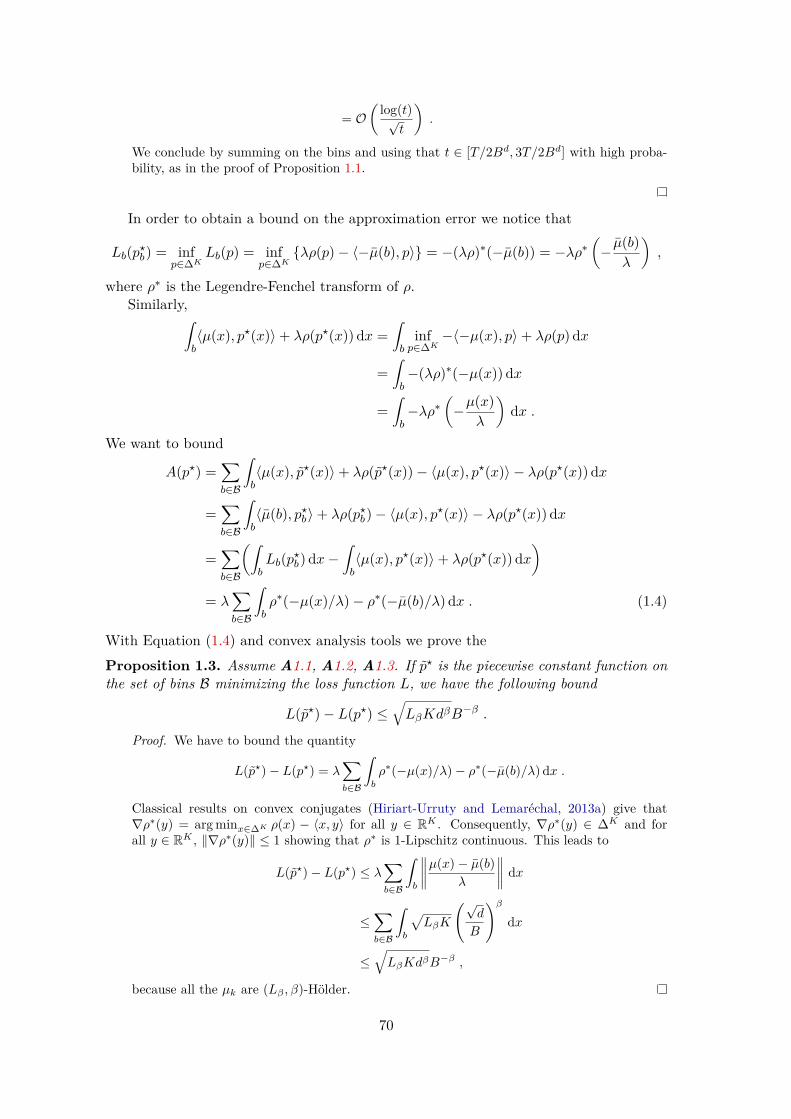
= O(

log(t)√t

).

We conclude by summing on the bins and using that t ∈ [T/2Bd, 3T/2Bd] with high proba-bility, as in the proof of Proposition 1.1.

In order to obtain a bound on the approximation error we notice that

Lb(p?b) = infp∈∆K

Lb(p) = infp∈∆K

λρ(p)− 〈−µ(b), p〉 = −(λρ)∗(−µ(b)) = −λρ∗(− µ(b)

λ

),

where ρ∗ is the Legendre-Fenchel transform of ρ.Similarly,∫

b〈µ(x), p?(x)〉+ λρ(p?(x)) dx =

∫b

infp∈∆K

−〈−µ(x), p〉+ λρ(p) dx

=∫b−(λρ)∗(−µ(x)) dx

=∫b−λρ∗

(−µ(x)

λ

)dx .

We want to bound

A(p?) =∑b∈B

∫b〈µ(x), p?(x)〉+ λρ(p?(x))− 〈µ(x), p?(x)〉 − λρ(p?(x))dx

=∑b∈B

∫b〈µ(b), p?b〉+ λρ(p?b)− 〈µ(x), p?(x)〉 − λρ(p?(x))dx

=∑b∈B

(∫bLb(p?b) dx−

∫b〈µ(x), p?(x)〉+ λρ(p?(x))dx

)= λ

∑b∈B

∫bρ∗(−µ(x)/λ)− ρ∗(−µ(b)/λ) dx . (1.4)

With Equation (1.4) and convex analysis tools we prove theProposition 1.3. Assume A1.1, A1.2, A1.3. If p? is the piecewise constant function onthe set of bins B minimizing the loss function L, we have the following bound

L(p?)− L(p?) ≤√LβKdβB

−β .

Proof. We have to bound the quantity

L(p?)− L(p?) = λ∑b∈B

∫b

ρ∗(−µ(x)/λ)− ρ∗(−µ(b)/λ) dx .

Classical results on convex conjugates (Hiriart-Urruty and Lemaréchal, 2013a) give that∇ρ∗(y) = arg minx∈∆K ρ(x) − 〈x, y〉 for all y ∈ RK . Consequently, ∇ρ∗(y) ∈ ∆K and forall y ∈ RK , ‖∇ρ∗(y)‖ ≤ 1 showing that ρ∗ is 1-Lipschitz continuous. This leads to

L(p?)− L(p?) ≤ λ∑b∈B

∫b

∥∥∥∥µ(x)− µ(b)λ

∥∥∥∥ dx

≤∑b∈B

∫b

√LβK

(√d

B

)βdx

≤√LβKdβB

−β ,

because all the µk are (Lβ , β)-Hölder.

70

Combining Propositions 1.1 and 1.3 we obtain the following theorem

Theorem 1.1 (Slow rates). Assume A1.1, A1.2, A1.3 and that ρ is S-smooth. ApplyingAlgorithm 1.1 with choice B = Θ

((T/ log(T ))1/(2β+d)

)gives4 for all T ≥ 1,

R(T ) = OLβ ,β,K,d

( T

log(T )

)− β2β+d

.

Proposition 1.2 directly shows that the result of this theorem also holds when ρ is theentropy function.

The proof of this theorem consists in choosing a value of B balancing between theestimation and the approximation errors. Since β ∈ (0, 1], we see that the exponent ofthe convergence rate is below 1/2 and that the proposed rate is slower than T−1/2, hencethe denomination of slow rate.

Proof. We will denote by Ck with increasing values of k the constants. Since the regret isthe sum of the approximation error and the estimation error we obtain

R(T ) ≤√LβdβKB

−β + C1√KBd/2

√log(T )T

+Bd2S log(eT )

T

+ C2KBd

T+ 4Bd(1 + ‖λρ‖∞) exp

(− T

12Bd

).

With the choice of

B =(C2β

√Lβd

β/2−1)1/(β+d/2)

(T

log(T )

)1/(2β+d),

we find that the three last terms of the regret are negligible with respect to the first two.This gives

R(T ) = O((

3√KL

d/(4β+2d)β dβ(4+d)/(4β+2d)(C2β)−β/(2β+d)

)( T

log(T )

)−β/(2β+d)).

When λ = 0 we are in the usual contextual bandit setting. The propositions of thissection hold and we recover the slow rates from (Perchet and Rigollet, 2013).

1.4.2 Fast rates

We now consider possible fast rates i.e., convergence rates faster than O(T−1/2). Theprice to pay to obtain these quicker rates compared to the ones from Section 1.4.1 is tohave problem-dependent bounds i.e., convergence rates depending on the parameters ofthe problem, and especially on λ.

As in the previous section we can obtain a bound on the estimation error based onthe convergence rates of the Upper-Confidence Frank-Wolfe algorithm.

This result needs additional assumptions, namely strong convexity and the followingassumption that we will make in the rest of this section. It consists in assuming that theminimum of the loss function on each bin is reached far from the boundaries of ∆K .

4The notation OLβ ,β,K,d means that there is a hidden constant depending on Lβ , β,K and d. Theconstant can be found in the proof.

71

A1.4. There exists η > 0 such that for all b ∈ B, dist(p?b , ∂∆K) ≥ η, where p?b is the pointwhere Lb : p 7→ 〈µ(b), p〉+ λ(b)ρ(p) attains its minimum.

Proposition 1.4. Assume A1.1, A1.2, A1.3, A1.4 and that ρ is ζ-strongly convex andS-smooth. Then running Algorithm 1.1 gives the following estimation error for all T ≥ 1,

EL(pT )− L(p?) = O(Bd(Sλ+ K

λ2ζ2η4

) log2(T )T

).

Proof. The proof is very similar to the one of Proposition 1.1. We decompose the estimationerror on the bins:

EL(pT )− L(p?) = 1Bd

∑b∈B

ELb(pT (b))− Lb(p?b) .

Let us now consider a single bin b ∈ B. We have run the UCB Frank-Wolfe algorithm for thefunction Lb on the bin b with Tb samples.

As in the proof of Proposition 1.1 we consider the event A.(Berthet and Perchet, 2017, Theorem 7) applied to Lb which is a λS-smooth λζ-strongly

convex function shows that on event A:

EL(pT )− L(p?) ≤ 2c1log2(T )T/Bd

+ 2c2log(T )T/Bd

+ c32

T/Bd,

with c1 = 96Kζλη2 , c2 = 24

ζλη3 + λS and c3 = 24(

20ζλη2

)2K + λζη2

2 + λS. Consequently

EL(pT )− L(p?) ≤ 2c1log2(T )T/Bd

+ 2c2log(T )T/Bd

+ c32

T/Bd+ 4Bd(1 + ‖λρ‖∞) exp

(− T

12Bd

).

In order to have a simpler expression we can use the fact that λ and η are constants that canbe small while S can be large. Consequently c3 is the largest constant among c1, c2 and c3and we obtain

EL(pT )− L(p?) ≤ O((

K

λ2ζ2η4 + Sλ

)Bd

log2(T )T

),

because the other terms are negligible.

The previous bound depends on several parameters of the problem: λ, distance η ofthe optimum to the boundary of the simplex, strong convexity and smoothness constants.Since λ can be arbitrarily small, η can be small as well and S large. Therefore the“constant” factor can explode despite the convergence rate being “fast”: these termsdescribe only the dependency in T .

As in the previous section we want to consider regularization functions ρ that are notsmooth on ∂∆K . To do so we force the vectors p to be inside the simplex by pre-samplingall arms at the beginning of the algorithm. The following lemma shows that this is valid.

Lemma 1.2. On a bin b ∈ B if there exists α ∈ (0, 1/2] and po ∈ ∆K such that p?b αpo(component-wise) then for all i ∈ [K], the agent can safely sample arm i αpoiT times atthe beginning of the algorithm without changing the convergence results.

The intuition behind this lemma is that if all arms have to be sampled a linear amountof times to reach the optimum value, it is safe to pre-sample each of the arms linearly atthe beginning of the algorithm. The goal is to ensure that the current proportion vectorpt will always be far from the boundary in order to leverage the smoothness of ρ in theinterior of the simplex.

72

Proof. We consider a single bin b ∈ B. Let us consider the function

Lb : p 7→ Lb(αpo + (1− α)p) .

Since for all i, p?b,i ≥ αpoi and since ∆K is convex we know that minp∈∆K Lb(p) = Lb(p?b).If p is the frequency vector obtained by running the UCB-Frank Wolfe algorithm for

function Lb with (1− α)T samples then minimizing Lb is equivalent to minimizing L with apresampling stage.

Consequently the whole analysis on the regret still holds with T replaced by (1 − α)T .Thus fast rates are kept with a constant factor 1/(1− α) ≤ 2.

Proposition 1.5. If ρ is the entropy function, sampling each arm Te−1/λ/K times duringthe presampling phase guarantees the same estimation error as in Proposition 1.4 withconstant S = Ke1/λ.

Proof. For the entropy regularization, we have

p?b,i = exp(−µ(b)i/λ)∑Kj=1 exp(−µ(b)j/λ)

≥ exp(−1/λ)K

.

We apply Lemma 1.2 with po =(

1K, . . . ,

1K

)and α = exp(−1/λ). Consequently each arm

is presampled T exp(−1/λ)/K times and finally we have

∀i ∈ [K], pi ≥exp(−1/λ)

K.

Therefore we have∀i ∈ [K], ∇iiρ(p) = 1

pi≤ K exp(1/λ) ,

showing that ρ is K exp(1/λ)-smooth.

In order to obtain faster rates for the approximation error we use Equation (1.4) andthe fact that ∇ρ∗ is 1/ζ-Lipschitz since ρ is ζ-strongly convex.

Proposition 1.6. Assume A1.1, A1.2, A1.3 and that ρ is ζ-strongly convex. If p? isthe piecewise constant function on the set of bins B minimizing the loss function L, thefollowing bound on the approximation error holds

L(p?)− L(p?) ≤ LβKdβ

2ζλ B−2β .

In order to prove Proposition 1.6 we will need the following lemma which is a directconsequence of a result on smooth convex functions.

Lemma 1.3. Let f : Rd → R be a convex function of class C1 and L > 0. Let g : Rd 3x 7→ L

2 ‖x‖2 − f(x). Then g is convex if and only if ∇f is L-Lipschitz continuous.

Proof. Since g is continuously differentiable we can write

g convex ⇔ ∀x, y ∈ Rd, g(y) ≥ g(x) + 〈∇g(x), y − x〉

⇔ ∀x, y ∈ Rd,L

2 ‖y‖2 − f(y) ≥ L

2 ‖x‖2 − f(x) + 〈Lx−∇f(x), y − x〉

⇔ ∀x, y ∈ Rd, f(y) ≤ f(x) + 〈∇f(x), y − x〉+ L

2

(‖y‖2 + ‖x‖2 − 2〈x, y〉

)⇔ ∀x, y ∈ Rd, f(y) ≤ f(x) + 〈∇f(x), y − x〉+ L

2 ‖x− y‖2

⇔ ∇f is L-Lipschitz continuous,

where the last equivalence comes from (Nesterov, 2004, Theorem 2.1.5).

73

We can now prove Proposition 1.6.

Proof. Since ρ is ζ-strongly convex then ∇ρ∗ is 1/ζ-Lipschitz continuous (see for example(Hiriart-Urruty and Lemaréchal, 2013b, Theorem 4.2.1, page 82)). Since ρ∗ is also convex,Lemma 1.3 shows that g : x 7→ 1

2ζ ‖x‖2 − ρ∗(x) is convex.

Let us now consider the bin b and the function µ = (µ1, . . . , µk). Jensen’s inequalitygives:

1|b|

∫b

g(−µ(x)/λ) dx ≥ g(

1|b|

∫b

−µ(x)λ

dx).

This leads to ∫b

g(−µ(x)/λ)dx ≥∫b

g(−µ(b)/λ) dx∫b

12ζ ‖−µ(x)‖2 /λ2 − ρ∗(−µ(x)/λ)dx ≥

∫b

12ζ ‖−µ(b)‖2 /λ2 − ρ∗(−µ(b)/λ) dx∫

b

ρ∗(−µ(x)/λ)− ρ∗(−µ(b)/λ)dx ≤ 12ζλ2

∫b

‖µ(x)‖2 − ‖µ(b)‖2 dx .

We use the fact that∫b‖µ(x)− µ(b)‖2 dx =

∫b‖µ(x)‖2 + ‖µ(b)‖2 − 2〈µ(x), µ(b)〉 dx =∫

b‖µ(x)‖2 + ‖µ(b)‖2 dx − 2〈µ(b),

∫bµ(x) dx〉 =

∫b‖µ(x)‖2 + ‖µ(b)‖2 dx − 2〈µ(b), |b|µ(b)〉 =∫

b

∥∥µ(x)2∥∥− ‖µ(b)‖2 dx and we get finally∫

b

ρ∗(−µ(x)/λ)− ρ∗(−µ(b)/λ) dx ≤ 12ζλ2

∫b

‖µ(x)− µ(b)‖2 dx .

Equation (1.4) shows that

L(p?)− L(p?) ≤ 12ζλ

∑b∈B

∫b

‖µ(b)− µ(x)‖2 dx

≤∑b∈B

∫b

LβK

2ζλ

(√d

B

)2β

dx

≤ LβKdβ

2ζλ

(1B

)2β,

because each µk is (Lβ , β)-Hölder.

Combining Propositions 1.4 and 1.6, we obtain fast rates for our problem.

Theorem 1.2 (Fast rates). Assume A1.1, A1.2, A1.3, A1.4 and that ρ is ζ-strongly con-vex and S-smooth. Then applying Algorithm 1.1 with the choice B = Θ

(T/ log2(T )

)1/(2β+d)

gives the following bound on the regret for all T ≥ 1,5

R(T ) = OLβ ,β,K,d,λ,η,ζ,S

( T

log2(T )

)− 2β2β+d

.

Proof. We denote again by Ck the constants. We sum the approximation and the estimationerrors (given in Propositions 1.6 and 1.4) to obtain the following bound on the regret:

R(T ) ≤ C1LβKd

β

ζλB−2β + C2

log2(T )T

Bd(

1ζλη3 + K

ζ2λ2η4 + λζη2 + λS

)+ 4Bd(1 + ‖λρ‖∞) exp

(− T

12Bd

).

5The precise dependency in the constants is again given in the proof below.

74

For the sake of clarity let us note ξ1 , C1LβKd

β

ζλand ξ2 , C2

(1

ζλη3 + K

ζ2λ2η4 + λζη2 + λS

).

We have

R(T ) ≤ ξ1B−2β + ξ2Bd log2(T )

T+ 4Bd(1 + ‖λρ‖∞) exp

(− T

12Bd

).

Taking

B =(

2ξ1βξ2

)1/(2β+d)(T

log2(T )

)1/(d+2β),

we notice that the third term is negligible and we conclude that

R(T ) = O(

2ξ1(

2ξ1βξ2

)−2β/(2β+d)(T

log2(T )

)−2β/(2β+d)).

The rate of Theorem 1.2 matches the rates obtained in nonparametric estimation (Tsy-bakov, 2008). However, as shown in the proof this fast rate is obtained at the price ofa factor involving λ, η and S, which can be arbitrarily large. It is the goal of the nextsection to see how to remove this dependency in the parameters of the problem.

Proposition 1.5 shows that the previous theorem can also be applied to the entropyregularization.

1.5 Convergence rates for non-constant λIn this section, we study the case where λ is a function of the context value and do notassume any more A1.3. This is quite interesting as agents might want to modulate theweight of the regularization term depending on the context.

1.5.1 Estimation and approximation errors

Equation (1.2) implies that the estimation errors obtained in Propositions 1.1 and 1.4are still correct if λ is replaced by λ(b). This is unfortunately not the case for theapproximation error propositions because Equation (1.4) does not hold anymore. Indeedthe approximation error becomes

A(p?) =∑b∈B

∫b〈µ(x), p?(x)〉+ λ(x)ρ(p?(x))− 〈µ(x), p?(x)〉 − λ(x)ρ(p?(x))dx

=∑b∈B

∫b〈µ(b), p?b〉+ λ(x)ρ(p?b)− 〈µ(x), p?(x)〉 − λ(x)ρ(p?(x))dx

=∑b∈B

(∫bLb(p?b) dx−

∫b〈µ(x), p?(x)〉+ λ(x)ρ(p?(x))dx

)=∑b∈B

∫b−(λ(b)ρ)∗(−µ(b)) + (λ(x)ρ)∗(−µ(x))dx

=∑b∈B

∫bλ(x)ρ∗

(−µ(x)λ(x)

)− λ(b)ρ∗

(− µ(b)λ(b)

)dx . (1.5)

The main difference with Equation (1.4) is that λ is not constant anymore. From thisexpression we obtain the following slow and fast rates of convergence. These rates are thesame as in Section 1.4 in term of the powers of B but have worse dependency in λ.

75

Proposition 1.7. If ρ is a strongly convex function and λ a C∞ integrable non-negativefunction whose inverse is also integrable, we have on a bin b:∫

b(λ(x)ρ)∗ (−µ(x))− (λ(b)ρ)∗ (−µ(b)) dx = O(Lβdβ/2B−β−d) .

We begin with a lemma on convex conjugates that will help us proving Proposition 1.7.

Lemma 1.4. Let λ, µ > 0 and let y ∈ Rn and ρ a non-negative convex function on ∆K .Then

(λρ)∗(y)− (µρ)∗(y) ≤ |λ− µ| ‖ρ‖∞ .

Proof. Let λ, µ > 0 and let y ∈ Rn. (λρ)∗(y) = supx∈∆K 〈x, y〉 − λρ(x) , 〈xλ, y〉 − λρ(xλ),where xλ ∈ ∆K is the point where the supremum of the concave problem is reached.

And (µρ)∗(y) = supx∈∆K 〈x, y〉 − µρ(x) , 〈xµ, y〉 − µρ(xµ) ≥ 〈xλ, y〉 − µρ(xλ), wherexµ ∈ ∆K is defined as above.

Then, (λρ)∗(y)− (µρ)∗(y) ≤ 〈xλ, y〉 − λρ(xλ)− (〈xλ, y〉 − µρ(xλ)) = (µ− λ)ρ(xλ).Finally (λρ)∗(y) − (µρ)∗(y) ≤ |λ − µ| ‖ρ‖∞, because ρ is continuous hence bounded on

the compact set ∆K .

Proof of Proposition 1.7. There exists x0 ∈ b such that λ(b) = λ(x0) and x1 ∈ b such thatµ(b) = µ(x1). We use Lemma 1.4 to derive a bound for the approximation error.∫

b

(λ(x)ρ)∗ (−µ(x))− (λ(b)ρ)∗ (−µ(b)) dx

=∫b

(λ(x)ρ)∗ (−µ(x))− (λ(x)ρ)∗ (−µ(b)) dx+∫b

(λ(x)ρ)∗ (−µ(b))− (λ(b)ρ)∗ (−µ(b)) dx

≤∫b

λ(x)(ρ∗(−µ(x)λ(x)

)− ρ∗

(− µ(b)λ(x)

))dx+

∫b

|λ(x)− λ(b)| ‖ρ‖∞ dx

≤∫b

λ(x)∣∣∣∣µ(x)λ(x) −

µ(b)λ(x)

∣∣∣∣ dx+ ‖ρ‖∞∫b

|λ(x)− λ(x0)| dx

≤∫b

Lβ |x− x1|β dx+ ‖ρ‖∞∫b

‖λ′‖∞ |x− x0| dx

≤ B−d(Lβd

β/2B−β + ‖ρ‖∞ ‖λ′‖∞√dB−1

)= O(B−β−d) .

The important point is that the bound does not depend on λmin, which is not the casewhen we want to obtain fast rates for the approximation error.

In order to do that we need a stronger assumption on λ than the one made by A1.2

A1.5. λ is a C∞ non-negative integrable function whose inverse is also integrable.

Proposition 1.8. Assume A1.1, A1.5 and that ρ is a ζ-strongly convex function. Thenwe have on each bin b ∈ B:∫

b(λ(x)ρ)∗ (−µ(x))− (λ(b)ρ)∗ (−µ(b)) dx = O

(KdL2

β ‖∇λ‖2∞B−2β−d

ζλ3min

).

For clarity reasons we postpone the proof to Appendix 1.A.1.The rate in B is improved compared to Proposition 1.7 at the expense of the constant

1/λ3min which can unfortunately be arbitrarily high.

76

1.5.2 Margin condition

We begin by giving a precise definition of the function η, the distance of the optimum tothe boundary of ∆K .

Definition 1.6. Let x ∈ X a context value. We define by p?(x) ∈ ∆K the point where(p 7→ 〈µ(x), p〉+ λ(x)ρ(p)) attains its minimum, and

η(x) := dist(p?(x), ∂∆K) .

Similarly, if p?b is the point where Lb : p 7→ 〈µ(b), p〉 + λ(b)ρ(p) attains its minimum, wedefine

η(b) := dist(p?b , ∂∆K) .

The fast rates obtained in Section 1.4.2 provide good theoretical guarantees but maybe useless in practice since they depend on a constant that can be arbitrarily large. Wewould like to discard the dependency on the parameters, and especially λ (that controlsη and S).

We begin by proving that η is β-Hölder continuous.

Lemma 1.5 (Regularity of η). Assume A1.1, A1.2 and that ρ is a ζ-strongly convexfunction. If η is the distance of the optimum p? to the boundary of ∆K as defined inDefinition 1.6, then η is β-Hölder. More precisely we have, for all bin b ∈ B

∀(x, y) ∈ b2, |η(x)− η(y)| ≤√

K

K − 1‖λ‖∞ + ‖λ′‖∞ζλmin(b)2 ‖x− y‖β = CL

λmin(b)2 ‖x− y‖β .

Proof. Let x ∈ X . Since η(x) = dist(p?b , ∂∆K) we obtain

η(x) =√

K

K − 1 minip?i (x) .

And

p?(x) = arg min 〈µ(x), p(x)〉+ λ(x)ρ(p(x)) = ∇(λ(x)ρ)∗(−µ(x)) = ∇ρ∗(−µ(x)λ(x)

).

Since ρ is ζ-strongly convex, ∇ρ∗ is 1/ζ-Lipschitz continuous.Let b ∈ B. We have, for (x, y) ∈ b2,

|p?(x)− p?(y)| ≤ 1ζ

∣∣∣∣µ(x)λ(x) −

µ(y)λ(y)

∣∣∣∣≤ 1ζ

∣∣∣∣µ(x)− µ(y)λ(x)

∣∣∣∣+ 1ζ|µ(y)|

∣∣∣∣ 1λ(x) −

1λ(y)

∣∣∣∣≤ 1ζλmin(b) ‖x− y‖

β + 1ζ

‖λ′‖∞λmin(b)2 ‖x− y‖ ,

since all µk are bounded by 1 (the losses are bounded by 1).

Difficulties arise when λ and η take values that are very small, meaning for instancethat we consider nearly no regularization. This is not likely to happen since we do wantto study contextual bandits with regularization. To formalize that we make an additionalassumption, which is common in nonparametric regression (Tsybakov, 2008) and is knownas a margin condition:

77

A1.6 (Margin Condition). We assume that there exist δ1 > 0 and δ2 > 0, α > 0 andCm > 0 such that∀δ ∈ (0, δ1], PX(λ(x) < δ) ≤ Cmδ6α and ∀δ ∈ (0, δ2], PX(η(x) < δ) ≤ Cmδ6α .

The non-negative parameter α controls the importance of the margin condition. Thepresence of a factor 6 is most likely a proof artifact.

The margin condition limits the number of bins on which λ or η can be small. There-fore we split the bins of B into two categories, the “well-behaved bins” on which λ and ηare not too small, and the “ill-behaved bins” where λ and η can be arbitrarily small. Theidea is to use the fast rates on the “well-behaved bin” and the slow rates (independent ofλ and η) on the “ill-behaved bins”. This is the point of Section 1.5.3.

Let CL =√

K

K − 1‖λ‖∞ + ‖∇λ‖∞

ζ, c1 = 1 + ‖∇λ‖∞ dβ/6 and c2 = 1 + CLd

β/2.

We define the set of “well-behaved bins” WB asWB = b ∈ B, ∃ x1 ∈ b, λ(x1) ≥ c1B

−β/3 and ∃ x2 ∈ b, η(x2) ≥ c2B−β/3 ,

and the set of “ill-behaved bin” as its complementary set in B.With the smoothness and regularity Assumptions 1.1 and 1.2, we derive lower bounds

for λ and η on the “well-behaved bins”.Lemma 1.6. Assume A1.1 and A1.2 and that ρ is a ζ-strongly convex function. If b isa well-behaved bin then

∀x ∈ b, λ(x) ≥ B−β/3 and ∀x ∈ b, η(x) ≥ B−β/3 .Proof. We consider a well-behaved bin b. There exists x1 ∈ b such that λ(x1) ≥ c1B

−β/3.Since λ is C∞ on [0, 1]d, it is in particular Lipschitz-continuous on b. And therefore∀x ∈ b, λ(x) ≥ c1B−β/3 − ‖λ′‖∞ diam(b) ≥ c1B−β/3 − ‖λ′‖∞ diam(b)β/3 = B−β/3 .

Lemma 1.5 shows that η is β-Hölder continuous (with constant denoted by CL/λ2min) and

therefore we have

∀x ∈ b, η(x) ≥ c2B−β/3 −CL

λmin(b)2 diam(b)β = B−β/3 .

1.5.3 Intermediate rates

We summarize the different error rates obtained in the previous sections.

Table 1.1 – Slow and Fast Rates for Estimation and Approximation Errors on a Bin

Error Slow Fast

Estim. B−d/2

√log(T )T

log2(T )T

(Sλ+ 1

η4λ2

)Approx. B−dB−β

B−2β−d

λ3

B

(T

log(T )

) 12β+d

(T

log2(T )

) 12β+d

R(T )(

T

log(T )

) −β2β+d

(T

log2(T )

) −2β2β+d

78

For the sake of clarity we removed the dependency on the bin, writing λ instead ofλ(b), and we only kept the relevant constants, that can be very small (λ and η), or verylarge (S).

Table 1.1 shows that the slow rates do not depend on the constants, so that we canuse them on the “ill-behaved bins”.

Theorem 1.3 (Intermediate rates). Assume A1.1, A1.2, A1.6 with parameter α ∈(0, 1) and that ρ is the entropy function. Applying Algorithm 1.1 with the choice B =

Θ(T/ log2(T )

) 12β+d gives the following bound of the regret for all T ≥ 1,

R(T ) = OK,d,α,β,Lβ

(T

log2(T )

)− β2β+d (1+α)

.

As explained in the proof in Appendix 1.A.2 we use a pre-sampling stage on each binto force the entropy to be smooth, as in the proofs of Propositions 1.2 and 1.5.

We consider now the extreme values of α. If α→ 0, there is no margin condition andthe speed obtained is T−

β2β+d which is exactly the slow rate from Theorem 1.1. If α→ 1,

there is a strong margin condition and the rate of Theorem 1.3 tends to T−2β

2β+d whichis the fast rate from Theorem 1.2. Consequently we get that the intermediate rates fromTheorem 1.3 do interpolate between the slow and fast rates obtained previously.

1.6 Lower boundsThe results in Theorems 1.1 and 1.2 have optimal exponents in the dependency in T .For the slow rate, since the regularization can be equal to 0, or a linear form, the lowerbounds on contextual bandits in this setting apply (Audibert et al., 2007; Rigollet andZeevi, 2010), matching this upper bound. For the fast rates, the following lower boundholds, based on a reduction to nonparametric regression (Tsybakov, 2008; Györfi et al.,2006).

Theorem 1.4. For any algorithm with bandit input and output pT , for ρ that is 1-stronglyconvex, we have

infp

supµ∈Hβ

ρ∈1-str. conv.

E[L(pT )]− L(p?)

≥ C T−

2β2β+d ,

for a universal constant C.

Proof. We consider the model withK = 2 where µ(x) = (−η(x), η(x))>, where η is a β-Hölderfunction on X = [0, 1]d. We note that η is uniformly bounded over X as a consequence ofsmoothness, so one can take λ such that |η(x)| < λ. We denote by e = (1/2, 1/2) the centerof the simplex, and we consider the loss

L(p) =∫X

(〈µ(x), p(x)〉+ λ‖p(x)− e‖2

)dx .

Denoting by p0(x) the vector e+ µ(x)/(2λ), we have that p0(x) ∈ ∆2 for all x ∈ X . Further,we have that

〈µ(x), p(x)〉+ λ‖p(x)− e‖2 = λ‖p(x)− p0(x)‖2 + 1/(4λ)‖µ(x)‖2 ,

79

since 〈µ(x), e〉 = 0. As a consequence, L is minimized at p0 and

L(p)− L(p0) =∫Xλ‖p(x)− p0(x)‖2 dx = 1/(2λ)

∫X|η(x)− η0(x)|2 dx ,

where η is such that p(x) =(1/2 − η(x)/(2λ), 1/2 + η(x)/(2λ)

). As a consequence, for any

algorithm with final variable pT , we can construct an estimator ηT such that

E[L(pT )]− L(p0) = 1/(2λ)E∫X|ηT (x)− η0(x)|2 dx ,

where the expectation is taken over the randomness of the observations Yt, with expectation±η(Xt), with sign depending on the known choice πt = 1 or 2. As a consequence, anyupper bound on the regret for a policy implies an upper bound on regression over β-Hölderfunctions in dimension d, with T observations. This yields that, in the special case where ρis the 1-strongly convex function equal to the squared `2-norm

infp

supµ∈Hβρ= `2

2

E[L(pT )]− L(p0) ≥ infη

supη∈Hβ

1/(2λ)E∫X|ηT (x)− η0(x)|2 dx ≥ CT−

2β2β+d .

The final bound is a direct application of (Györfi et al., 2006, Theorem 3.2).

The upper and lower bound match up to logarithmic terms. This bound is obtainedfor K = 2, and the dependency of the rate in K is not analyzed here.

1.7 Empirical resultsWe present in this section experiments and simulations for the regularized contextualbandits problem. The setting we consider usesK = 3 arms, with an entropy regularizationand a fixed parameter λ = 0.1. We run successive experiments for values of T rangingfrom 1 000 to 100 000, and for different values of the smoothness parameter β. The arms’rewards follow 3 different probability distributions (Poisson, exponential and Bernoulli),with β-Hölder mean functions.

The results presented in Figure 1.1 shows that (T 7→ T · R(T )) growths as expected,and the lower β, the slower the convergence rate, as shown on the graph.

0 25,000 50,000 75,000 100,000

500

1,000

1,500

T

R(T

)·T

β = 0.3β = 0.5β = 0.7β = 0.9

Figure 1.1 – Regret as a Function of T

In order to verify that the fast rates proven in Section 1.4.2 are indeed reached, weplot on Figure 1.2 the ratio between the regret and the theoretical bound on the regret

80

(T/ log2(T )

)− 2β2β+d . We observe that this ratio is approximately constant as a function of

T , which validates empirically the theoretical convergence rates.

0 25,000 50,000 75,000 100,000

0.05

0.1

0.15

0.20

0.25

0.30

T

R(T

)(T/

log2 (

T))−

2β/(2β

+d)

β = 0.3β = 0.5β = 0.7β = 0.9

Figure 1.2 – Normalized Regret as a Function of T

1.8 ConclusionWe proposed an algorithm for the problem of contextual bandits with regularizationreaching fast rates similar to the ones obtained in nonparametric estimation, and validatedby our experiments. We can discard the parameters of the problem in the convergencerates by applying a margin condition that allows us to derive intermediate convergencerates interpolating perfectly between the slow and fast rates.

1.A Proof of the intermediate rates resultsIn this section we prove Proposition 1.8 and Theorem 1.3.

1.A.1 Proof of Proposition 1.8Proof of Proposition 1.8. As in the proof of Proposition 1.6 we consider a bin b ∈ B and thegoal is to bound ∫

b

λ(x)ρ∗(−µ(x)λ(x)

)− λ(b)ρ∗

(− µ(b)λ(b)

)dx .

We use a similar method and we apply Jensen inequality with density λ(x)|b|λ(b)

to the function

g : x 7→ 12ζ ‖x‖

2 − ρ∗(x) which is convex.

g

(∫b

−µ(x)λ(x)

λ(x)|b|λ(b)

dx)≤∫b

g

(−µ(x)λ(x)

)λ(x)|b|λ(b)

dx

g

(− µ(b)λ(b)

)≤∫b

g

(−µ(x)λ(x)

)λ(x)|b|λ(b)

dx

12ζ

∥∥∥∥− µ(b)λ(b)

∥∥∥∥2− ρ∗

(− µ(b)λ(b)

)≤ 1|b|λ(b)

∫b

[12ζ

∥∥∥∥−µ(x)λ(x)

∥∥∥∥2− ρ∗

(−µ(x)λ(x)

)]λ(x) dx

∫b

λ(x)ρ∗(−µ(x)λ(x)

)− λ(b)ρ∗

(− µ(b)λ(b)

)dx ≤ 1

2ζ

∫b

‖µ(x)‖2

λ(x) − ‖µ(b)‖2

λ(b)dx .

81

Consequently we have proven that∫b

λ(x)ρ∗(−µ(x)λ(x)

)− λ(b)ρ∗

(− µ(b)λ(b)

)dx ≤ 1

2ζ

∫b

‖µ(x)‖2

λ(x) − ‖µ(b)‖2

λ(b)dx

≤ 12ζ

K∑k=1

∫b

µk(x)2

λ(x) −µk(b)2

¯λ(b)dx .

Therefore we have to bound, for each k, I =∫b

µk(x)2

λ(x) −µk(b)2

λ(b)dx.

Let us omit the subscript k and consider a β-Hölder function µ.We have

I =∫b

µ(x)2

λ(x) −µ(b)2

λ(b)dx

=∫b

µ(x)2

λ(x) −µ(x)2

λ(b)+ µ(x)2

λ(b)− µ(b)2

λ(b)dx

=∫b

(µ(x)2 − µ(b)2)( 1

λ(x) −1λ(b)

)dx︸ ︷︷ ︸

I1

+∫b

µ(b)2(

1λ(x) −

1λ(b)

)dx︸ ︷︷ ︸

I2

+∫b

1λ(b)

(µ(x)2 − µ(b)2) dx︸ ︷︷ ︸

I3

.

We now have to bound these three integrals.

(a) Bounding I1:

I1 =∫b

(µ(x)2 − µ(b)2)( 1

λ(x) −1λ(b)

)dx

=∫b

(µ(x) + µ(b)) (µ(x)− µ(b))(

1λ(x) −

1λ(b)

)dx

≤∫b

2|µ(x)− µ(b)|∣∣∣∣ 1λ(x) −

1λ(b)

∣∣∣∣ dx≤ 2Lβ

(√d

B

)β ∫b

∣∣∣∣ 1λ(x) −

1λ(b)

∣∣∣∣ dx .Since 1/λ is of class C1, Taylor-Lagrange inequality yields, using the fact that there existsx0 ∈ b such that λ(b) = λ(x0)∣∣∣∣ 1

λ(x) −1λ(b)

∣∣∣∣ ≤∥∥∥∥∥(

1λ

)′∥∥∥∥∥∞

|x− x0| ≤‖λ′‖∞λ2

min

√d

B.

We obtain therefore

I1 ≤ 2Lβ ‖λ′‖∞√dβ+1 1

λ2min

B−(1+β+d) = O(B−(1+β+d)

λ2min

).

(b) Bounding I2:

We haveI2 = µ(b)2

∫b

(1

λ(x) −1λ(b)

)dx ≤

∫b

(1

λ(x) −1λ(b)

)dx ,

82

because∫b

(1

λ(x) −1λ(b)

)dx ≥ 0 from Jensen’s inequality.

Without loss of generality we can assume that the bin b is the closed cuboid [0, 1/B]d. Wesuppose that for all x ∈ b, λ(x) > 0.Since λ is of class C∞, we have the following Taylor series expansion

λ(x) = λ(0) +d∑i=1

∂λ(0)∂xi

xi + 12∑i,j

∂2λ(0)∂xi∂xj

xixj + O(‖x‖2) .

Integrating over the bin b we obtain

λ(b) = λ(0) + 12

1B

d∑i=1

∂λ(0)∂xi

+ 18

1B2

∑i6=j

∂2λ(0)∂xi∂xj

+ 16

1B2

d∑i=1

∂2λ(0)∂x2

i

+ O

(1B2

).

Consequently∫b

dxλ(b)

= 1Bdλ(b)

= 1Bdλ(0)

1

1 + 12λ(0)

1B

d∑i=1

∂λ(0)∂xi

+ 1λ(0)

1B2

18∑i 6=j

∂2λ(0)∂xi∂xj

+ 16

d∑i=1

∂2λ(0)∂x2

i

+ O

(1B2

)

= 1Bdλ(0)

(1− 1

2λ(0)1B

d∑i=1

∂λ(0)∂xi

− 1λ(0)

1B2

18∑i 6=j

∂2λ(0)∂xi∂xj

+ 16

d∑i=1

∂2λ(0)∂x2

i

+ 1

4λ(0)21B2

(d∑i=1

∂λ(0)∂xi

)2

+ O

(1B2

))

= 1Bdλ(0) −

12λ(0)2

1Bd+1

d∑i=1

∂λ(0)∂xi

− 1λ(0)2

1Bd+2

18∑i 6=j

∂2λ(0)∂xi∂xj

+ 16

d∑i=1

∂2λ(0)∂x2

i

+ 1

4λ(0)31

Bd+2

(d∑i=1

∂λ(0)∂xi

)2

+ O

(1B2

).

Let us now compute the Taylor series development of 1/λ. We have

∂

∂xi

1λ(x) = − 1

λ(x)2∂λ(x)∂xi

and ∂2

∂xi∂xj

1λ(x) = − 1

λ(x)2∂2λ(x)∂xi∂xj

+ 2λ(x)3

∂λ(x)∂xi

∂λ(x)∂xj

.

This lets us write

1λ(x) = 1

λ(0) −1

λ(0)2

d∑i=1

∂λ(0)∂xi

xi −12

1λ(0)2

∑i,j

∂2λ(0)∂xi∂xj

xixj + 1λ(0)3

∑i,j

∂λ(0)∂xi

∂λ(0)∂xj

xixj + O(‖x‖2)

∫b

dxλ(x) = 1

λ(0)1Bd− 1

2λ(0)21

Bd+1

d∑i=1

∂λ(0)∂xi

− 1λ(0)2

1Bd+2

18∑i6=j

∂2λ(0)∂xi∂xj

+ 16

d∑i=1

∂2λ(0)∂x2

i

+ 1λ(0)3

1Bd+2

14∑i6=j

∂λ(0)∂xi

∂λ(0)∂xj

+ 13

d∑i=1

(∂λ(0)∂xi

)2+ O

(1

Bd+2

).

And then

I2 ≤112

1λ(0)3

1Bd+2

d∑i=1

(∂λ(0)∂xi

)2+ O

(1

Bd+2

).

83

Since the derivatives of λ are bounded we obtain that

I2 = O(B−2−d

λ3min

).

(c) Bounding I3:

I3 =∫b

1λ(b)

(µ(x)2 − µ(b)2) dx

= 1λ(b)

∫b

(µ(x)− µ(b))2 dx

≤ 1λmin

L2βd

βB−(2β+d) = O(B−(2β+d)

λmin

).

Putting I1, I2 and I3 together we have I = O(

(dL2β ‖∇λ‖

2∞)B

−(2β+d)

λ3min

). And finally

L(p?)− L(p?) = O(KdL2

β ‖∇λ‖2∞B−2β

ζλ3min

).

1.A.2 Proof of Theorem 1.3

Before proving the theorem, we need a simple lemma.

Lemma 1.7. If ρ is convex, η is an increasing function of λ.

Proof. As in the proof of Proposition 1.2 we use the KKT conditions to find that on a bin b(without the index k for the arm):

µ(b) + λ(b)∇ρ(p?b) + ξ = 0 .

Thereforep?b = (∇ρ)−1

(−ξ + µ(b)

λ(b)

).

Since ρ is convex, ∇ρ is an increasing function and its inverse as well. Consequently p?b is anincreasing function of λ(b), and since η(b) =

√K/(K − 1) mini p?b,i, η is also an increasing

function of λ(b).

Proof of Theorem 1.3. Since B will be chosen as an increasing function of T we only considerT sufficiently large in order to have c1B−β/3 < δ1 and c2B

−β/3 < δ2. To ensure this wecan also take smaller δ1 and δ2. Moreover we lower the value of δ2 or δ1 to be sure thatδ2c2

= η( δ1c1

). These are technicalities needed to simplify the proof.The proof will be divided into several steps. We will first obtain lower bounds on λ and η

for the “well-behaved bins”. Then we will derive bounds for the approximation error and theestimation error. And finally we will put that together to obtain the intermediate convergencerates.

As in the proofs on previous theorems we will denote the constants Ck with increasingvalues of k. We divide the rest of the proof into 4 steps.

(a) Lower bounds on η and λ:Using a technique from (Rigollet and Zeevi, 2010) we notice that without loss of generalitywe can index the Bd bins with increasing values of λ(b). Let us note IB = 1, . . . , j1 andWB = j1 + 1, . . . , Bd. Since η is an increasing function of λ (cf Lemma 1.7), the η(bj) arealso increasingly ordered.

84

Let j2 ≥ j1 be the largest integer such that λ(bj) ≤δ1c1

. Consequently we also have that j2 is

the largest integer such that η(bj) ≤δ2c2

.

Let j ∈ j1 + 1, . . . , j2. The bin bj is a well-behaved bin and Lemma 1.6 shows thatλ(bj) ≥ B−β/3. Then λ(bj) + (c1 − 1)B−β/3 ≤ c1λ(bj) ≤ δ1 and we can apply the margincondition (cf Assumption 1.6) which gives

PX(λ(x) ≤ λ(bj) + (c1 − 1)B−β/3) ≤ Cm(c1λ(bj))6α .

But since the context are uniformly distributed and since the λ(bj) are increasingly orderedwe also have that

PX(λ(x) ≤ λ(bj) + (c1 − 1)B−β/3) ≥ PX(λ(x) ≤ λ(bj)) ≥j

Bd.

This gives λ(bj) ≥1

c1C1/6αm

(j

Bd

)1/6α. The same computations give η(bj) ≥

1c2C

1/6αm

(j

Bd

)1/6α.

We note Cγ , min((c1C1/6αm )−1, (c2C1/6α

m )−1)) and γj , Cγ

(j

Bd

)1/α. Consequently λ(bj) ≥

γj and η(bj) ≥ γj .Let us now compute the number of ill-behaved bins:

#b ∈ B, b /∈ WB = Bd P(b /∈ WB)= Bd P(∀x ∈ B, η(x) ≤ c2B−β/3 or ∀x ∈ B, λ(x) ≤ c1B−β/3)≤ Bd P(η(x) ≤ c2B−β/3 or λ(x) ≤ c1B−β/3)≤ Cm(c6α1 + c6α2 )BdB−2αβ , CIB

dB−2αβ ,

where x is the mean context value in the bin b. Consequently if j ≥ j? , CIBdB−2αβ , then

bj ∈ WB. Let j , CIBdB−αβ ≥ j?. Consequently for all j ≥ j?, bj ∈ WB.

We want to obtain an upper-bound on the constant S ¯λ(bj) + K

η(bj)4λ(bj)2that arises in the

fast rate for the estimation error. For the sake of clarity we will remove the dependency inbj and denote this constant C = Sλ+ K

λ2η4 .

In the case of the entropy regularization S = 1/mini p?i . Since η =√K/(K − 1) mini p?i , we

have that mini p?i =√

(K − 1)/Kη ≥ η/2. Consequently S ≤ 2/γj and, on a well-behavedbin bj , for j ≤ j2,

C ≤K + 2 ‖λ‖∞

γ6j

,CFγ6j

, (1.6)

where the subscript F stands for “Fast”. When j ≥ j2, we have λ(bj) ≥ δ1/c1 and η(bj) ≥δ2/c2 and consequently

C ≤ K

(δ1/c1)2(δ2/c2)4 + 2 ‖λ‖∞δ2/c2

, Cmax .

Let us notice than λ being known by the agent, the agent knows the value of λ(b) on each binb and can therefore order the bins. Consequently the agent can sample, on every well-behavedbin, each arm Tγj/2 times and be sure that mini pi ≥ γj/2. On the first

⌊j⌋bins the agent

will sample each arm λ(b)√T/Bd times as in the proof of Proposition 1.2.

(b) Approximation Error:We now bound the approximation error. We separate the bins into two sets: 1, . . . , bj?cand dj?e , . . . , Bd. On the first set we use the slow rates of Proposition 1.7 and on thesecond set we use the fast rates of Proposition 1.8.

85

We obtain that, for α < 1/2,

L(p?)− L(p?) ≤ Lβdβ/2bj?c∑j=1

B−β−d + ‖ρ‖∞ ‖∇λ‖∞√d

bj?c∑j=1

B−1−d

+ (KdL2β ‖∇λ‖

2∞)

Bd∑j=dj?e

B−2β−d

λ(bj)3

≤ CILβdβ/2B−βB−2αβ

+ (KdL2β ‖∇λ‖

2∞)

j2∑j=dj?e

B−2β−d

γ3j

+Bd∑

j=j2+1

B−2β−d

(c1/δ1)3

+ O(B−2αβ−β)

≤ CILβdβ/2B−2αβ−β

+ (KdL2β ‖∇λ‖

2∞)

B−2β−d

C3γ

j2∑j=dj?e

(j

Bd

)−1/2α+B−2β

(δ1c1

)3+ O(B−2αβ−β)

≤ CILβdβ/2B−2αβ−β

+ (KdL2β ‖∇λ‖

2∞) 1

C3γ

B−2β∫ 1

CIB−2αβx−1/2α dx+ O(B−2αβ−β)

≤

(CILβd

β/2 +KdL2β ‖∇λ‖

2∞

2α1− 2α

C(2α−1)/2αI

C3γ

)B−β−2αβ + O(B−2αβ−β)

= O(B−β−2αβ) ,

since α < 1/2. We step from line 3 to 4 thanks to a series-integral comparison.For α = 1/2 we get

L(p?)− L(p?) ≤(CILβd

β/2 +(KdL2

β ‖∇λ‖2∞

)(δ3

1c−31 + 2βC−3

γ log(B)))B−2β + O(B−2β)

= O(B−2β log(B)

).

And for α > 1/2 we have

L(p?)− L(p?) ≤(KdL2

β ‖∇λ‖2∞

)( 1C3γ

2α2α− 1 +

(δ1c1

)3)B−2β + O(B−2β) = O

(B−2β) ,

because β + 2αβ > 2β.Let us note

ξ1 ,

(CILβd

β/2 +KdL2β ‖∇λ‖

2∞

2α1− 2α

C(2α−1)/2αI

C3γ

);

ξ2 ,(CILβd

β/2 +(KdL2

β ‖∇λ‖2∞

)(δ3

1c−31 + 2βC−3

γ log(B)))

;

ξ3 ,(KdL2

β ‖∇λ‖2∞

)( 1C3γ

2α2α− 1 +

(δ1c1

)3)

;

ξapp , max(ξ1, ξ2, ξ3) .

Finally we obtain that the approximation error is bounded by ξappB−min(β+2αβ,2β) log(B)

with α > 0.(c) Estimation Error:We proceed in a similar manner as for the approximation error, except that we do not splitthe bins around j? but around j.

86

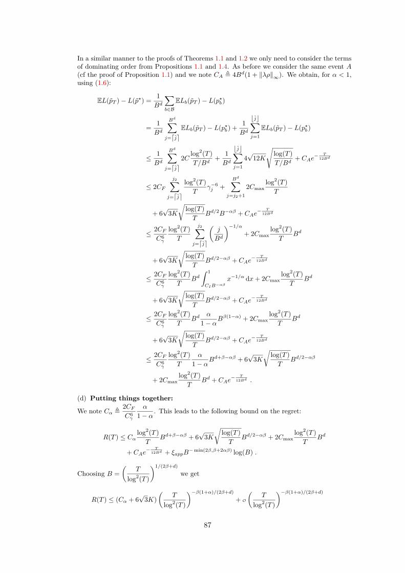
In a similar manner to the proofs of Theorems 1.1 and 1.2 we only need to consider the termsof dominating order from Propositions 1.1 and 1.4. As before we consider the same event A(cf the proof of Proposition 1.1) and we note CA , 4Bd(1 + ‖λρ‖∞). We obtain, for α < 1,using (1.6):

EL(pT )− L(p?) = 1Bd

∑b∈B

ELb(pT )− L(p?b)

= 1Bd

Bd∑j=dje

ELb(pT )− L(p?b) + 1Bd

bjc∑j=1

ELb(pT )− L(p?b)

≤ 1Bd

Bd∑j=dje

2C log2(T )T/Bd

+ 1Bd

bjc∑j=1

4√

12K

√log(T )T/Bd

+ CAe− T

12Bd

≤ 2CFj2∑

j=dje

log2(T )T

γ−6j +

Bd∑j=j2+1

2Cmaxlog2(T )T

+ 6√

3K√

log(T )T

Bd/2B−αβ + CAe− T

12Bd

≤ 2CFC6γ

log2(T )T

j2∑j=dje

(j

Bd

)−1/α+ 2Cmax

log2(T )T

Bd

+ 6√

3K√

log(T )T

Bd/2−αβ + CAe− T

12Bd

≤ 2CFC6γ

log2(T )T

Bd∫ 1

CIB−αβx−1/α dx+ 2Cmax

log2(T )T

Bd

+ 6√

3K√

log(T )T

Bd/2−αβ + CAe− T

12Bd

≤ 2CFC6γ

log2(T )T

Bdα

1− αBβ(1−α) + 2Cmax

log2(T )T

Bd

+ 6√

3K√

log(T )T

Bd/2−αβ + CAe− T

12Bd

≤ 2CFC6γ

log2(T )T

α

1− αBd+β−αβ + 6

√3K√

log(T )T

Bd/2−αβ

+ 2Cmaxlog2(T )T

Bd + CAe− T

12Bd .

(d) Putting things together:

We note Cα ,2CFC6γ

α

1− α . This leads to the following bound on the regret:

R(T ) ≤ Cαlog2(T )T

Bd+β−αβ + 6√

3K√

log(T )T

Bd/2−αβ + 2Cmaxlog2(T )T

Bd

+ CAe− T

12Bd + ξappB−min(2β,β+2αβ) log(B) .

Choosing B =(

T

log2(T )

)1/(2β+d)we get

R(T ) ≤ (Cα + 6√

3K)(

T

log2(T )

)−β(1+α)/(2β+d)+ O

(T

log2(T )

)−β(1+α)/(2β+d)

87

which is valid for α ∈ (0, 1).Finally we have

R(T ) = O((

T

log2(T )

)−β(1+α)/(2β+d)).

88

2 Online A-optimal design and active lin-ear regression

We consider in this chapter the problem of optimal experiment design where a deci-sion maker can choose which points to sample to obtain an estimate β of the hiddenparameter β? of an underlying linear model. The key challenge of this work lies in thefact that we allow heteroscedasticity, meaning that each covariate can have a differentand unknown variance. The goal of the decision maker is then to figure out on thefly the optimal way to allocate the total budget of T samples between covariates, assampling several times a specific one will reduce the variance of the estimated modelaround it (but at the cost of a possible higher variance elsewhere). By trying to mini-mize the `2-loss E[‖β−β?‖2] the decision maker is actually minimizing the trace of thecovariance matrix of the problem, which corresponds then to online A-optimal design.Combining techniques from bandit and convex optimization we propose a new activesampling algorithm and we compare it with existing ones. We provide theoreticalguarantees of this algorithm in different settings, including a O(T−2) regret boundin the case where the covariates form a basis of the feature space, generalizing andimproving existing results. Numerical experiments validate our theoretical findings1.

2.1 Introduction and related workA classical problem in statistics consists in estimating an unknown quantity, for examplethe mean of a random variable, parameters of a model, poll results or the efficiency of amedical treatment. In order to do that, statisticians usually build estimators which arerandom variables based on the data, supposed to approximate the quantity to estimate. Away to construct an estimator is to make experiments and to gather data on the estimand.In the polling context an experiment consists for example in interviewing people in order toknow their voting intentions. However if one wants to obtain a “good” estimator, typicallyan unbiased estimator with low variance, the choice of which experiment to run has to bedone carefully. Interviewing similar people might indeed lead to a poor prediction. In thiswork we are interested in the problem of optimal design of experiments, which consistsin choosing adequately the experiments to run in order to obtain an estimator with smallvariance. We focus here on the case of heteroscedastic linear models with the goal of

1This chapter is joint work with Pierre Perrault, Michal Valko and Vianney Perchet. It has led to thefollowing publication:(Fontaine et al., 2019b) Online A-Optimal Design and Active Linear Regression, Xavier Fontaine,Pierre Perrault, Michal Valko and Vianney Perchet, submitted.

89

actively constructing the design matrix. Linear models, though possibly sometimes toosimple, have been indeed widely studied and used in practice due to their interpretabilityand can be a first good approximation model for a complex problem.

The original motivation of this problem comes from use cases where obtaining the labelof a sample is costly, hence choosing carefully which points to sample in a regression taskis crucial. Consider for example the problem of controlling the wear of manufacturingmachines in a factory (Antos et al., 2010), which requires a long and manual process.The wear can be modeled as a linear function of some features of the machine (age,number of times it has been used, average temperature, ...) so that two machines withthe same parameters will have similar wears. Since the inspection process is manual andcomplicated, results are noisy and this noise depends on the machine: a new machine,slightly worn, will often be in a good state, while the state of heavily worn machines canvary a lot. Thus evaluating the linear model for the wear requires additional examinationsof some machines and less inspection of others. Another motivating example comes fromeconometrics, typically in income forecasting. It is usually assumed that the annualincome is influenced by the individual’s education level, age, gender, occupation, etc.through a linear model. Polling is also an issue in this context: what kind of individual topoll to gain as much information as possible about an explanatory variable? Finally thesetting we investigate is also relevant to the design of nuclear fusion experiments (Stoianet al., 2013), which are costly, and require the parametrization of a large quantity ofdynamic variables (to control the target quality and the temporal laser pulse shape).Using machine learning techniques to reach a controlled thermonuclear fusion can onlybe done on small size experiment history. It is therefore crucial to design the experiencesin order to improve the predictive model in the best possible way.

The field of optimal experiment design (Pukelsheim, 2006) aims precisely at choosingwhich experiment to perform in order to minimize an objective function within a budgetconstraint. In experiment design, the distance of the produced hypothesis to the true oneis measured by the covariance matrix of the error (Boyd and Vandenberghe, 2004). Thereare several criteria that can be used to minimize a covariance matrix, the most popularbeing A, D and E-optimality. In this chapter we focus on A-optimal design whose goalis to minimize the trace of the covariance matrix. Contrary to several existing workswhich solve the A-optimal design problem in an offline manner in the homoscedastic set-ting (Sagnol, 2010; Yang et al., 2013; Gao et al., 2014) we are interested here in proposingan algorithm which solves this problem sequentially, with the additional challenge thateach experiment has an unknown and different variance.

Our problem is therefore close to “active learning” which is more and more popularnowadays because of the exponential growth of datasets and the cost of labeling data.Indeed, the latter may be tedious and require expert knowledge, as in the domain ofmedical imaging. It is therefore essential to choose wisely which data to collect and tolabel, based on the information gathered so far. Usually, machine learning agents areassumed to be passive in the sense that the data is seen as a fixed and given input thatcannot be modified or optimized. However, in many cases, the agent can be able toappropriately select the data (Goos and Jones, 2011). Active learning specifically studiesthe optimal ways to perform data selection (Cohn et al., 1996) and this is crucial as oneof the current limiting factors of machine learning algorithms are computing costs, thatcan be reduced since all examples in a dataset do not have equal importance (Freundet al., 1997). For example Bordes et al. (2005) proposed a SVM algorithm where exampleselection yields faster training and higher accuracy compared to classical passive SVMtechniques. This approach has many practical applications: in online marketing where

90

one wants to estimate the potential impact of new products on customers, or in onlinepolling where the different options do not have the same variance (Atkeson and Alvarez,2018).

There exist different variants of active learning (perhaps depending on the differentunderstandings of the word “active”). Maybe the most common one is the so-called“pool-based” active learning (McCallumzy and Nigamy, 1998), where the decision makerhas access to a pool of examples and chooses which one to query and to label. Anothervariant is the “retraining-based” active learning (Yang and Loog, 2016) whose principleis to retrain the model on well-chosen examples, for instance the ones that had the higheruncertainty. Castro and Nowak (2008) have proven general minimax bounds for activelearning, for a general class of functions, with rates depending on noise conditions andon the regularity of the decision boundary (see also Tosh and Dasgupta (2017); Hannekeand Yang (2015)).

In this chapter we consider therefore a decision maker who has a limited experimentalbudget of T ≥ 1 samples and who aims at learning some latent linear model. The goalis to build a predictor β that estimates the unknown parameter of the linear modelβ?, and that minimizes E[‖β − β?‖2]. The key point here is that the design matrix isconstructed sequentially and actively by the agent: at each time step, the decision makerchooses a “covariate” Xk ∈ Rd and receives a noisy output X>k β? + ε. The quality of thepredictor is measured through its variance. The agent will repeatedly query the differentavailable covariates in order to obtain more precise estimates of their values. Instinctivelya covariate with small variance should not be sampled too often since its value is alreadyquite precise. On the other hand, a noisy covariate will be sampled more often. The majorissue lies in the heteroscedastic assumption: the unknown variances must be learned towisely sample the points.

Antos et al. (2010) introduced a specific variant of our setting where the environmentproviding the data is assumed to be stochastic and i.i.d. across rounds. More precisely,they studied this problem using the framework of stochastic multi-armed bandits (MAB)by considering a set of K probability distributions (or arms), associated with K variances.Their objective is to define an allocation strategy over the arms to estimate their expectedvalues uniformly well. Later, the analysis and results have been improved by Carpentieret al. (2011). However, this line of work is actually focusing on the case where thecovariates are only vectors of the canonical basis of Rd, which gives a simpler closed formlinear regression problem.

There have been some recent works on MAB with heteroscedastic noise (Cowan et al.,2017; Kirschner and Krause, 2018) with natural connections to this chapter. Indeed,covariates could somehow be interpreted as contexts in contextual bandits. The mostrelated setting might be the one of Soare (2015). However, they are mostly concernedabout best-arm identification while recovering the latent parameter β? of the linear modelis a more challenging task (as each decision has an impact on the loss). In that sense weimprove the results of Soare (2015) by proving a bound on the regret of our algorithm.Other works as (Chen and Price, 2019) propose active learning algorithms aiming atfinding a constant factor approximation of the classification loss while we are focusing onthe statistical problem of recovering β?. Yet another similar setting has been introducedin (Riquelme et al., 2017a). In this setting the agent has to estimate several linearmodels in parallel and for each covariate (that appears randomly), the agent has to decidewhich model to estimate. Other works studied the problem of active linear regression,and for example Sugiyama and Rubens (2008) proposed an algorithm conducting activelearning and model selection simultaneously but without any theoretical guarantees. More

91

recently Riquelme et al. (2017b) have studied the setting of active linear regression withthresholding techniques in the homoscedastic case. An active line of research has also beenconducted in the domain of random design linear regression (Hsu et al., 2011; Sabato andMunos, 2014; Dereziński et al., 2019). In these works the authors aim at controllingthe mean-squared regression error E[(X>β − Y )2] with a minimum number of randomsamples Xk. Except from the loss function that they considered, these works differ fromours in several points: they generally do not consider the heteroscedastic case and theirgoal is to minimize the number of samples to use to reach an ε-estimator while in oursetting the total number of covariates K is fixed. Allen-Zhu et al. (2020) provide a similaranalysis but under the scope of optimal experiment design. Another setting similar toours is introduced in (Hazan and Karnin, 2014), where active linear regression with ahard-margin criterion is studied. However, the minimization of the classical `2-norm ofthe difference between the true parameter of the linear model and its estimator seems tobe a more natural criterion, which justifies our investigations.

In this work we adopt a different point of view from the aforementioned existingworks. We consider A-optimal design under the heteroscedasticity assumption and wegeneralize MAB results to the non-coordinate basis setting with two different algorithmstaking inspiration from the convex optimization and bandit literature. We prove optimalO(T−2) regret bounds for d covariates and provide a weaker guarantee for more thand covariates. Our work emphasizes the connection between MAB and optimal design,closing open questions in A-optimal design. Finally we corroborate our theoretical findingswith numerical experiments.

The remainder of this chapter is organized as follows. We describe the setting of ourproblem in Section 2.2, then we present a naive algorithm in Section 2.3 and a fasteralgorithm in Section 2.4. We discuss the case K > d in Section 2.5 and present numericalsimulations in Section 2.6. Finally Section 2.7 concludes the chapter. Appendix 2.Acontains the postponed proofs.

2.2 Setting and description of the problem

2.2.1 Motivations and description of the setting

Let X1, . . . , XK ∈ Rd beK covariates available to some agent who can successively sampleeach of them (several times if needed). Observations Y are generated by a standard linearmodel, i.e.,

Y = X>β? + ε with β? ∈ Rd .

Each of these covariates correspond to an experiment that can be run by the decisionmaker to gain information about the unknown vector β?. The goal of optimal experimentdesign is to choose the experiments to perform from a pool of possible design pointsX1, . . . , XK in order to obtain the best estimate β of β? within a fixed budget ofT ∈ N∗ samples. In classical experiment design problems the variances of the differentexperiments are supposed to be equal. Here we consider the more challenging settingwhere each covariate has a specific and unknown variance σ2

k, i.e., we suppose that whenXk is queried for the i-th time the decision maker observes

Y(i)k = X>k β

? + ε(i)k ,

where E[ε(i)k ] = 0, Var[ε(i)

k ] = σ2k > 0 and ε(i)

k is κ2-subgaussian. We assume also that theε

(i)k are independent from each other. This setting corresponds actually to online optimal

92

experiment design since the decision maker has to design sequentially the sampling policy,in an adaptive manner.

A naive sampling strategy would be to sample the covariates Xk with the static ho-moscedastic proportions. In our heteroscedastic setting, this will not produce the mostprecise estimate of β? because of the different variances σ2

k. Intuitively a point Xk with alow variance will provide very precise information on the value X>k β? while a point witha high variance will not give much information (up to the converse effect of the norm‖Xk‖). This indicates that a point with high variance should be sampled more often thana point with low variance. Since the variances σ2

k are unknown, we need at the same timeto estimate σ2

k (which might require lots of samples of Xk to be precise) and to minimizethe estimation error (which might require only a few examples of some covariate Xk).There is then a trade-off between gathering information on the values of σ2

k and usingit to optimize the loss; the fact that this loss is global, and not cumulative, makes thistrade-off “exploration vs. exploitation” much more intricate than in standard multi-armedbandits.

Usual algorithms handling global losses are rather slow (Agrawal and Devanur, 2014;Mannor et al., 2014) or dedicated to specific well-posed problems with closed form losses (An-tos et al., 2010; Carpentier et al., 2011). Our setting can be seen as an extension of thetwo aforementioned works that aim at estimating the means of a set of K distributions.Noting µ = (µ1, . . . , µK)> the vector of the means of those distributions and Xi = ei theith vector of the canonical basis of RK , we see (since X>i µ = µi) that their objective isactually to estimate the parameter µ of a linear model. This setting is a particular caseof ours since the vectors Xi form the canonical basis of RK .

2.2.2 Definition of the loss function

As we mentioned it before, the decision maker can be led to sample several times thesame design point Xk in order to obtain a more precise estimate of its response X>k β?.We denote therefore by Tk ≥ 0 the number of samples of Xk, hence T = ∑K

k=1 Tk. Foreach k ∈ [K]2, the linear model yields the following

T−1k

Tk∑i=1

Y(i)k = XT

k β? + T−1

k

Tk∑i=1

ε(i)k .

We define Yk = ∑Tki=1 Y

(i)k /σk

√Tk , Xk =

√TkXk/σk and εk = ∑Tk

i=1 ε(i)k /σk

√Tk so that

for all k ∈ [K], Yk = XTk β

? + εk, where E[ε] = 0 and Var[εk] = 1. We denote byX = (X>1 , · · · , X>K)> ∈ RK×d the induced design matrix of the policy. Under the as-sumption that X has full rank, the above Ordinary Least Squares (OLS) problem has anoptimal unbiased estimator β = (X>X)−1X>Y . The overarching objective is to upper-bound E[‖β − β?‖2], which can be easily rewritten as follows:

E[‖β − β?‖2

]= Tr((X>X)−1) = Tr

(K∑k=1

XkX>k

)−1

= 1TTr(

K∑k=1

pkXkX>k /σ

2k

)−1

,

where we have denoted for every k ∈ [K], pk = Tk/T the proportion of times the covariateXk has been sampled. By definition, p = (p1, . . . , pK) ∈ ∆K , the simplex of dimensionK − 1. We emphasize here that minimizing E[‖β − β?‖2] is equivalent to minimizing

2[K] = 1, . . . ,K.

93

the trace of the inverse of the covariance matrix X>X, which corresponds actually toA-optimal design (Pukelsheim, 2006). Denote now by Ω(p) the following weighted matrix

Ω(p) =K∑k=1

pkσ2k

XkX>k = X>X .

The objective is to minimize over p ∈ ∆K the loss function L(p) = Tr(Ω(p)−1) with

L(p) = +∞ if (p 7→ Ω(p)) is not invertible, such that

E[‖β − β?‖2

]= 1TTr(Ω(p)−1

)= 1TL(p) .

For the problem to be non-trivial, we require that the covariates span Rd. If it is not thecase then there exists a vector along which one cannot get information about the param-eter β?. The best algorithm we can compare against can only estimate the projection ofβ on the subspace spanned by the covariates, and we can work in this subspace.

The rest of this work is devoted to design an algorithm minimizing Tr(Ω(p)−1) with

the difficulty that the variances σ2k are unknown. In order to do that we will sequentially

and adaptively choose which point to sample to minimize Tr(Ω(p)−1). This corresponds

consequently to online A-optimal design. As developed above, the norms of the covariateshave a scaling role and those can be renormalized to lie on the sphere at no cost, which isthus an assumption from now on: ∀k ∈ [K], ‖Xk‖2 = 1. The following proposition showsthat the problem we are considering is convex.

Proposition 2.1. L is strictly convex on ∆d and continuous in its relative interior ∆d.

Proof. Let p, q ∈ ∆d, so that Ω(p) and Ω(q) are invertible, and λ ∈ [0, 1]. We have L(p) =Tr(Ω(p)−1) and L(λp+ (1− λ)q) = Tr(Ω(λp+ (1− λ)q)−1), where

Ω(λp+ (1− λq)) =d∑k=1

λpk + (1− λ)qkσ2k

XkX>k = λΩ(p) + (1− λ)Ω(q).

It is well-known (Whittle, 1958) that the inversion is strictly convex on the set of positivedefinite matrices. Consequently,

Ω(λp+ (1− λq))−1 = (λΩ(p) + (1− λ)Ω(q))−1 ≺ λΩ(p)−1 + (1− λ)Ω(q)−1 .3

Taking the trace this gives

L(λp+ (1− λ)q) < λL(p) + (1− λ)L(q).

Hence L is strictly convex.

Proposition 2.1 implies that L has a unique minimum p? in ∆d and we note

p? = arg minp∈∆d

L(p) .

Finally, we evaluate the performance of a sampling policy in term of “regret” i.e., thedifference in loss between the optimal sampling policy and the policy in question.

Definition 2.1. Let pT denote the sampling proportions after T samples of a policy. Itsregret is then

R(T ) = 1T

(E [L(pT )]− L(p?)) .3where ≺ denotes the strict Loewner ordering between symmetric matrices.

94

We will construct active sampling algorithms to minimize R(T ). A key step is thefollowing computations of the gradient of L. Since ∇kΩ(p) = XkX

Tk /σ

2k, it follows

∂pkL(p) = − 1σ2k

Tr(Ω(p)−2XkX

Tk

)= − 1

σ2k

∥∥∥Ω(p)−1Xk

∥∥∥2

2.

As in several works (Hsu et al., 2011; Allen-Zhu et al., 2020) we will have to study differentcases depending on the values of K and d. The first one corresponds to the case K ≤ d.As we explained it above, ifK < d, the matrix Ω(p) is not invertible and it is impossible toobtain a sublinear regret, which makes us work in the subspace spanned by the covariatesXk. This corresponds to K = d. We will treat this case in Sections 2.3 and 2.4. The caseK > d is considered in Section 2.5.

2.2.3 Concentration arguments

Before going on with algorithms to solve the problem described in Section 2.2.2, wepresent results on the concentration of the variance for subgaussian random variables.Traditional results on the concentration of the variances (Maurer and Pontil, 2009; Car-pentier et al., 2011) are obtained in the bounded setting. We propose results in a moregeneral framework. Let us begin with some definitions.

Definition 2.2 (Sub-gaussian random variable). A random variable X is said to be κ2-sub-gaussian if

∀λ ≥ 0, exp(λ(X − EX)) ≤ exp(λ2κ2/2) .And we define its ψ2-norm as

‖X‖ψ2= inf

t > 0 |E[exp(X2/t2)] ≤ 2

.

We can bound the ψ2-norm of a subgaussian random variable as stated in the followinglemma.

Lemma 2.1 (ψ2-norm). If X is a centered κ2-sub-gaussian random variable then

‖X‖ψ2≤ 2√

2√3κ .

Proof. A proposition stated in (Wainwright, 2019) shows that for all λ ∈ [0, 1), a sub-gaussianvariable X verifies

E(λX2

2κ2

)≤ 1√

1− λ.

Taking λ = 3/4 and defining u = 2√

2√3 κ gives

E(X2/u2) ≤ 2 .

Consequently ‖X‖ψ2≤ u.

A wider class of random variables is the class of sub-exponential random variablesthat are defined as follows.

Definition 2.3 (Sub-exponential random variable). A random variable X is said to besub-exponential if there exists K > 0 such that

∀ 0 ≤ λ ≤ 1/K, E[exp(λ|X|)] ≤ exp(Kλ) .

And we define its ψ1-norm as

‖X‖ψ1= inf t > 0 |E[exp(|X|/t)] ≤ 2 .

95

A result from (Vershynin, 2018) gives the following lemma, that makes a connectionbetween subgaussian and subexponential random variables.

Lemma 2.2. A random variable X is sub-gaussian if and only if X2 is sub-exponential,and we have ∥∥∥X2

∥∥∥ψ1

= ‖X‖2ψ2.

We now want to obtain a concentration inequality on the empirical variance of a sub-gaussian random variable. We give use the following notations to define the empiricalvariance.

Definition 2.4. We define the following quantities for n i.i.d. repetitions of the randomvariable X.

µ = E[X] and µn = 1n

n∑i=1

Xi ,

µ(2) = E[X2] and µ(2)n = 1

n

n∑i=1

X2i .

The variance and empirical variance are defined as follows

σ2 = µ(2) − µ2 and σ2n = µ(2)

n − µ2n .

We are now able to state the main result of this section.

Theorem 2.1. Let X be a centered and κ2-sub-gaussian random variable sampled n ≥ 2times. Let δ ∈ (0, 1). Let c = (e−1)(2e(2e−1))−1 ≈ 0.07. With probability at least 1− δ,the following concentration bound on its empirical variance holds

∣∣∣σ2n − σ2

∣∣∣ ≤ 3κ2 ·max

log(4/δ)cn

,

√log(4/δ)cn

.

This theorem provides a concentration result on the empirical variance of a subgaus-sian random variable, whereas usual concentration bounds are generally obtained forbounded random variables (Maurer and Pontil, 2009; Carpentier et al., 2011), for whichthe concentration bound is easier to obtain.

Proof. We have ∣∣σ2n − σ2∣∣ =

∣∣∣µ(2)n − µ2

n − (µ(2) − µ2)∣∣∣

≤∣∣∣µ(2)n − µ(2)

∣∣∣+∣∣µ2n − µ2∣∣

≤∣∣∣µ(2)n − µ(2)

∣∣∣+ |µn − µ||µn + µ|

≤∣∣∣µ(2)n − µ(2)

∣∣∣+ |µn|2

since µ = 0.We now apply Hoeffding’s inequality (Vershynin, 2018) to the Xt variables that are κ2-

subgaussian, to get

P

(1n

n∑i=1

Xi − µ > t

)≤ exp

(− n

2t2

2nκ2

)= exp

(−nt

2

2κ2

).

96

And finally

P

(|µn − µ| > κ

√2 log(2/δ)

n

)≤ δ.

Consequently with probability at least 1 − δ, |µn|2 ≤ 2κ2 log(2/δ)n

. The variables X2t are

sub-exponential random variables. We can apply Bernstein’s inequality as stated in (Chafaïet al., 2012) to get for all t > 0:

P

(∣∣∣∣∣ 1nn∑i=1

X2i − µ(2)

∣∣∣∣∣ > t

)≤ 2 exp

(−cnmin

(t2

s2 ,t

m

))≤ 2 exp

(−cnmin

(t2

m2 ,t

m

)).

with c = e−12e(2e−1) , s2 = 1

n

∑ni=1∥∥X2

i

∥∥ψ1≤ m2 and m = max1≤i≤n

∥∥X2i

∥∥ψ1. Inverting the

inequality we obtain

P

(∣∣∣µ(2)n − µ(2)

∣∣∣ > m ·max(

log(2/δ)cn

,

√log(2/δ)cn

))≤ δ.

And finally, with probability at least 1− δ,∣∣σ2n − σ2∣∣ ≤ m ·max

(log(4/δ)cn

,

√log(4/δ)cn

)+ 2κ2 log(4/δ)

n.

Using Lemmas 2.2 and 2.1 we obtain that m ≤ 8κ2/3. Finally,∣∣σ2n − σ2∣∣ ≤ 8

3κ2 ·max

(log(4/δ)cn

,

√log(4/δ)cn

)+ 2cκ2 log(4/δ)

cn

≤ 3κ2 ·max(

log(4/δ)cn

,

√log(4/δ)cn

),

since 2c ≤ 1/3. This gives the expected result.

We now state a corollary of this result.Corollary 2.1. Let T ≥ 2. Let X be a centered and κ2-sub-gaussian random variable.

Let c = (e − 1)(2e(2e − 1))−1 ≈ 0.07. For n =⌈

72κ4

cσ4 log(2T )⌉, we have with probability

at least 1− 1/T 2, ∣∣∣σ2n − σ2

∣∣∣ ≤ 12σ

2.

Proof. Let δ ∈ (0, 1). Let n =⌈

log(4/δ)c

(6κ2

σ2

)2⌉.

Then log(4/δ)cn

≤(σ2

6κ2

)2

< 1, since σ2 ≤ κ2, by property of subgaussian randomvariables.

With probability 1− δ, Theorem 2.1 gives

|σ2n − σ2| ≤ 3κ2 σ

2

6κ2 ≤12σ

2 .

Now, suppose that δ = 1/T 2. Then, with probability 1 − 1/T 2, for n =⌈

72κ4

cσ4 log(2T )⌉

samples,

|σ2n − σ2| ≤ 1

2σ2 .

97

2.3 A naive randomized algorithmWe begin by proposing an obvious baseline for the problem at hand. One naive algorithmwould be to estimate the variances of each of the covariates by sampling them a fixedamount of time. Sampling each arm cT times (with c < 1/K) would give an approximationσk of σk of order 1/

√T . Then we can use these values to construct Ω(p) an approximation

of Ω(p) and then derive the optimal proportions pk to minimize Tr(Ω(p)−1). Finally thealgorithm would consist in using the remainder of the budget to sample the arms accordingto those proportions. However, such a trivial algorithm would not provide good regretguarantees. Indeed the constant fraction c of the samples used to estimate the varianceshas to be chosen carefully; it will lead to a 1/T regret if c is too big (if c > p?k for somek). That is why we need to design an algorithm that will first roughly estimate the p?k. Inorder to improve the algorithm it will also be useful to refine at each iteration the estimatespk. Following these ideas we propose Algorithm 2.1 which uses a pre-sampling phase (seeLemma 2.6 for further details) and which constructs at each iteration lower confidenceestimates of the variances, providing an optimistic estimate L of the objective function L.Then the algorithm minimizes this estimate (with an offline A-optimal design algorithm,see e.g., (Gao et al., 2014)). Finally the covariate Xk is sampled with probability pt,k.Then feedback is collected and estimates are updated.

Algorithm 2.1 Naive randomized algorithmRequire: d, T , δ confidence parameterRequire: N1, . . . , Nd of sum N1: Sample Nk times each covariate Xk

2: pN ←− (N1/N, . . . , Nd/N)3: Compute empirical variances σ2

1, . . . , σ2d

4: for N + 1 ≤ t ≤ T do5: Compute pt ∈ arg min L, where L is the same function as L, but with variances

replaced by lower confidence estimates of the variances (from Theorem 2.1).6: Draw π(t) randomly according to probabilities pt and sample covariate Xπ(t)7: Update pt+1 = pt + 1

t+1(eπ(t+1) − pt) and σ2π(t) where (e1, . . . , ed) is the canonical

basis of Rd.

Proposition 2.2. For T ≥ 1 samples, running Algorithm 2.1 with Ni = poiT/2 (with podefined by (2.2)) for all i ∈ [K], gives final sampling proportions pT such that

R(T ) = OΓ,σk

(√log TT 3/2

),

where Γ is the Gram matrix of X1, . . . , XK .

Notice that we avoid the problem discussed by Erraqabi et al. (2017) (that is due toinfinite gradient on the simplex boundary) thanks to presampling, allowing us to havepositive empirical variance estimates with high probability.

Proof. We now conduct the analysis of Algorithm 2.1. Our strategy will be to convert theerror L(pT )− L(p?) into a sum over t ∈ [T ] of small errors. Notice first that for i ∈ [K], thequantity ∥∥Ω(p)−1Xi

∥∥22

98

can be upper bounded by 1σiλmin(Γ) maxk∈[K]

σ2k

0.5po , for p = pT , where we have denoted by

Γ the Gram matrix of X1, . . . , XK and where λmin(Γ) denotes the smallest eigenvalue of Γ.

For p = pt, we can also bound this quantity by 4σiλmin(Γ) maxk∈[K]

σ2k

0.5po , using Lemma 2.6to express pt with respect to lower estimates of the variances — and thus with respect to realvariance thanks to Corollary 2.1. Then using the convexity of L we have

L(pT )− L(p?) = L(pT )− L(

1/TT∑t=1

pt

)+ L

(1T

T∑t=1

pt

)− L(p?)

≤∑k

−∥∥∥∥Ω(pT )−1Xk

σk

∥∥∥∥2

2

(pk,T −

1T

T∑t=1

pk,t

)+ 1T

T∑t=1

(L(pt)− L(p?)) .

Using Hoeffding inequality,(pk,T − 1

T

∑Tt=1 pk,t

)= 1

T

∑Tt=1 (Ik is sampled at t − pk,t)

is bounded by√

log(2/δ)T with probability 1 − δ. It thus remains to bound the second term

1T

∑Tt=1 (L(pt)− L(p?)). First, notice that L(p) is an increasing function of σi for any i.

If we define L be replacing each σ2i by lower confidence estimates of the variances σ2

i (seeTheorem 2.1), then

L(pt)− L(p?) ≤ L(pt)− L(p?) = L(pt)− L(pt) + L(pt)− L(p∗) ≤ L(pt)− L(pt).

Since the gradient of L with respect to σ2 is(

2piσ3i

∥∥Ω(p)−1Xi

∥∥22

)i, we can bound L(pt)− L(pt)

by1/σ3

min supk

∥∥Ω(pt)−1Xk

∥∥22

∑i

2pi,t|σ2i − σ2

i | .

Since pi,t is the probability of having a feedback from covariate i, we can use the probabilisti-cally triggered arm setting of (Wang and Chen, 2017) to prove that 1

T

∑Tt=1∑i 2pi|σ2

i − σ2i | =

O(√

log(T )T

). Taking δ of order T−1 gives the desired result.

2.4 A faster first-order algorithmWe now improve the relatively “slow” dependency in T in the rates of Algorithm 2.1 –due to its naive reduction to a MAB problem, and because it does not use any estimatesof the gradient of L – with a different approach based on convex optimization techniques,that we can leverage to gain an order in the rates of convergence.

2.4.1 Description of the algorithm

The main algorithm is described in Algorithm 2.2 and is built following the work of Berthetand Perchet (2017). The idea is to sample the arm which minimizes a proxy of the gradientof L corrected by a negative error term, as in the UCB algorithm (Auer et al., 2002).

99

Algorithm 2.2 Bandit algorithmRequire: K, TRequire: N1, . . . , NK of sum N1: Sample Nk times each covariate Xk

2: pN ←− (N1/N, . . . , NK/N)3: Compute empirical variances σ2

1, . . . , σ2K

4: for N + 1 ≤ t ≤ T do5: Compute ∇L(pt), where L is the same function as L, but with variances replaced

by empirical variances.6: for k ∈ [K] do

7: gk ←− ∇kL(pt)− 2√

3 log(t)Tk

8: π(t)←− arg mink∈[d] gk and sample covariate Xπ(t)9: Update pt+1 = pt + 1

t+1(eπ(t+1) − pt) and update σ2π(t)

N1, . . . , NK are the number of times each covariate is sampled at the beginning of thealgorithm. This stage is needed to ensure that L is smooth. More details about that willbe given with Lemma 2.6.

2.4.2 Concentration of the gradient of the loss

The cornerstone of the algorithm is to guarantee that the estimates of the gradientsconcentrate around their true value. To simplify notations, we denote by Gk = ∂pkL(p)the true kth derivative of L and by Gk its estimate. More precisely, if we note Ω(p) =∑Kk=1(pk/σk )XkX

>k , we have

Gk = −σ−2k ‖Ω(p)−1Xk‖22 and Gk , −σ−2

k ‖Ω(p)−1Xk‖22 .

Since Gk depends on the σ2k, we need a concentration bound on the empirical variances

of sub-gaussian random variables.Using Theorem 2.1 we claim the following concentration argument, which is the main

ingredient of the analysis of Algorithm 2.2.

Proposition 2.3. For every k ∈ [K], after having gathered Tk ≤ T samples of covari-ates Xk, there exists a constant C > 0 (explicit and given in the proof) such that, withprobability at least 1− δ

|Gk − Gk| ≤ C

(σ−1k max

i∈[K]

σ2i

pi

)3

·max

log(4TK/δ)Tk

,

√log(4TK/δ)

Tk

.

For clarity reasons we postpone the proof to Appendix 2.A. Proving this propositionwas one of the main technical challenges of our analysis. Now that we have it proven wecan turn to the analysis of Algorithm 2.2.

2.4.3 Analysis of the convergence of the algorithm

In convex optimization several classical assumptions can be leveraged to derive fast con-vergence rates. Those assumptions are typically strong convexity, positive distance fromthe boundary of the constraint set, and smoothness of the objective function, i.e., that ithas Lipschitz gradient. We prove in the following that the loss L satisfies them, up to the

100

smoothness because its gradient explodes on the boundary of ∆d. However, L is smoothon the relative interior of the simplex. Consequently we will circumvent this smoothnessissue by using a technique from Chapter 1 consisting in pre-sampling every arm a linearnumber of times in order to force p to be far from the boundaries of ∆d.

We denote X0 , (X>1 , · · · , X>d )> and Γ , X0X>0 = Gram(X1, . . . , Xd). Noting alsoCof(M)ij the (i, j) cofactor of a matrixM and Com(M) the comatrix (matrix of cofactors)of M , we prove the following lemmas.

Lemma 2.3. The diagonal coefficients of Ω(p)−1 can be computed as follows:

∀i ∈ [d], Ω(p)−1ii =

d∑j=1

σ2j Cof(X>0 )2

ij

det(X>0 X0)1pj.

Proof. We suppose that ∀i ∈ [d], pi 6= 0 so that Ω(p) is invertible.

We know that Ω(p)−1 = Com(Ω(p))>det(Ω(p)) . We compute now det(Ω(p)).

det(Ω(p)) = det(

d∑k=1

pkXkX>k

σ2k

)= det((

√T−1X)>

√T−1X) = T−d det(X>)2

= T−d

∣∣∣∣∣∣∣∣∣...

X1... Xd

...

∣∣∣∣∣∣∣∣∣2

=

∣∣∣∣∣∣∣∣∣∣

...√p1

σ1X1

...√pd

σdXd

...

∣∣∣∣∣∣∣∣∣∣

2

= det(X0)2 p1

σ21· · · pd

σ2d

.

We now compute Com(Ω(p))ii.

Com(Ω(p)) = Com(T−1/2X>T−1/2X) = Com(T−1/2X>) Com(T−1/2X>)> .

Let us note M , T−1/2X =

· · ·

√p1

σ1X>1 · · ·...

· · ·√pK

σKX>K · · ·

. Therefore

Com(Ω(p))ii =d∑j=1

Com(M>)2ij =

d∑j=1

∏k 6=j

pkσ2k

Cof(X>0 )2ij .

Finally,

Ω(p)−1ii =

d∑j=1

σ2j Cof(X>0 )2

ij

det(X>0 X0)1pj

.

This allows us to derive the exact expression of the loss function L.

Lemma 2.4. The loss function L verifies for all p ∈ ∆d,

L(p) = 1det(X>0 X0)

d∑k=1

σ2k

pkCof(X0X>0 )kk .

101

Proof. Using Lemma 2.3 we obtain

L(p) = Tr(Ω(p)−1) =d∑k=1

Ω(p)−1kk

= 1det(X>X)

d∑k=1

σ2k

pk

d∑i=1

Cof(X>0 )2ik = 1

det(X>0 X0)

d∑k=1

σ2k

pkCom(X0X>0 )kk .

With this expression, the optimal proportion p? can be easily computed using theKKT theorem, with the following closed form:

p?k = σk

√Cof(Γ)kk/

d∑i=1

σi

√Cof(Γ)ii . (2.1)

This yields that L is strongly convex on ∆d, with strong convexity parameter

µ = 2 det(Γ)−1 mini

Cof(Γ)iiσ2i .

Moreover, this also implies that p? is far away from the boundary of ∆d.

Lemma 2.5. Let η , dist(p?, ∂∆d) be the distance from p? to the boundary of the simplex.Then

η =√

K

K − 1mini σi

√Cof(Γ)ii∑d

k=1 σk√

Cof(Γ)kk.

Proof. This is immediate with (2.1) since η =√

K

K − 1 mini p?i .

It remains to recover the smoothness of L. This is done using a pre-sampling phase.

Lemma 2.6 (see Lemma 1.2). If there exists α ∈ (0, 1/2] and po ∈ ∆d such that p? < αpo

(component-wise) then sampling arm i at most αpoiT times (for all i ∈ [d]) at the beginningof the algorithm and running Algorithm 2.2 is equivalent to running Algorithm 2.2 withbudget (1− α)T on the smooth function (p 7→ L(αpo + (1− α)p).

We have proved that p?k is bounded away from 0 and thus a pre-sampling would bepossible. However, this requires to have some estimate of each σ2

k. The upside is that thoseestimates must be accurate up to some multiplicative factor (and not additive factor) sothat a logarithmic number of samples of each arm is enough to get valid lower/upperbounds (see Corollary 2.1). Indeed, the estimate σ2

k obtained satisfies, for each k ∈ [d],that σ2

k ∈ [σ2k/2, 3σ2

k/2]. Consequently we know that

∀k ∈ [d], p?k ≥1√3

σk√

Cof(Γ)kk∑di=1 σi

√Cof(Γ)ii

≥ 12p

o, where po = σk√

Cof(Γ)kk∑di=1 σi

√Cof(Γ)ii

. (2.2)

This will let us use Lemma 2.6 and with a presampling stage as prescribed, p is forced toremain far away from the boundaries of the simplex in the sense that pt,i ≥ poi /2 at eachstage t subsequent to the pre-sampling, and for all i ∈ [d]. Consequently, this logarithmicphase of estimation plus the linear phase of pre-sampling ensures that in the rest of theprocess, L is actually smooth.

102

Lemma 2.7. With the pre-sampling of Lemma 2.6, L is smooth with constant CS where

CS ≤ 432σ2

max

(∑dk=1 σk

√Cof(Γ)kk

)3

det(Γ)σ3min√

mink Cof(Γ)kk.

Proof. We use the fact that for all i ∈ [d], pi ≥ poi /2. We have that for all i ∈ [d],

∇2iiL(p) = Cof(Γ)iiσ2

i

det(Γ)2p3i

≤ 2 Cof(Γ)iiσ2i

det(Γ)(poi /2)3 .

We have pok = σk√

Cof(Γ)kk∑di=1 σi

√Cof(Γ)ii

which gives

∇2iiL(p) ≤ 16

σ2max

(∑dk=1 σk

√Cof(Γ)kk

)3

det(Γ)σ3min√

mink Cof(Γ)kk, CS .

And consequently L is CS-smooth.We can obtain an upper bound on CS using Corollary 2.1, which tells that σk/2 ≤ σk ≤

3σk/2:

CS ≤ 432σ2

max

(∑dk=1 σk

√Cof(Γ)kk

)3

det(Γ)σ3min√

mink Cof(Γ)kk.

We can now state our main theorem.

Theorem 2.2. Applying Algorithm 2.2 with T ≥ 1 samples after having pre-sampled eacharm k ∈ [d] at most pokT/2 times gives the following bound4

R(T ) = OΓ,σk

(log2(T )T 2

).

This theorem provides a fast convergence rate for the regret R(T ) and emphasizes theimportance of using the gradient information in Algorithm 2.2 compared to Algorithm 2.1.

Proof. Proposition 2.3 gives that

|Gi− Gi| ≤ 678Kσmax

σ4min

(1

σiλmin(Γ) maxk∈[K]

σ2k

pk

)3

·κ2max ·max

log(4TK/δ)Ti

,

√log(4TK/δ)

Ti

.

Since each arm has been sampled at least a linear number of times we guarantee thatlog(4TK/δ)/Ti ≤ 1 such that

|Gi − Gi| ≤ 678K(σmax

σmin

)7 1λmin(Γ)3

κ2maxp3

min

√log(4TK/δ)

Ti.

Thanks to the presampling phase of Lemma 2.6, we know that pmin ≥ po/2. For the sake of

clarity we note C , 678K(σmax

σmin

)7 8po3λmin(Γ)3κ

2max such that |Gi−Gi| ≤ C

√log(4TK/δ)

Ti.

We have seen that L is µ-strongly convex, CL-smooth and that dist(p?, ∂∆d) ≥ η. Conse-quently, since Lemma 2.6 shows that the pre-sampling stage does not affect the convergence

4The notation OΓ,σk means that there is a hidden constant depending on Γ and on the σk. The explicitdependency on these parameters is given in the proof.

103

result, we can apply (Berthet and Perchet, 2017, Theorem 7) (with the choice δT = 1/T 2,which gives that

E[L(pT )]− L(p?) ≤ c1log2(T )T

+ c2log(T )T

+ c31T,

with c1 = 96C2K

µη2 , c2 = 24C2

µη3 +S and c3 = 30722K

µ2η4 ‖L‖∞+ µη2

2 +CS . With the presamplingstage and Lemma 2.4, we can bound ‖L‖∞ by

‖L‖∞ ≤∑j σ

2j Cof(Γ)jj

σmin√

Cof(Γ)min

∑j

σj

√Cof(Γ)jj

.

We conclude the proof using the fact that R(T ) = 1T

(L(pT )− L(p?)).

2.5 Discussion and generalization to K > d

We discuss in this section the case where the number K of covariate vectors is greaterthan d.

2.5.1 Discussion of the Case K > d

In the case where K > d it may be possible that the optimal p? lies on the boundaryof the simplex ∆K , meaning that some arms should not be sampled. This happens forinstance as soon as there exist two covariate points that are exactly equal but with differentvariances. The point with the lowest variance should be sampled while the point withthe highest one should not. All the difficulty of an algorithm for the case where K > dis to be able to detect which covariate should be sampled and which one should not. Inorder to adopt another point of view on this problem it might be interesting to go back tothe field of optimal design of experiments. Indeed by choosing vk = Xk/σk, our problemconsists exactly in the following constraint minimization problem given v1 . . . , vK ∈ Rd:

minTr

K∑j=1

pjvjv>j

−1

under contraints p ∈ ∆K . (P)

It is known (Pukelsheim (2006)) that the dual problem of A-optimal design consists infinding the smallest ellipsoid, in some sense, containing all the points vj :

maxTr(√W )2 under contraints W 05 and v>j Wvj ≤ 1 for all 1 ≤ j ≤ K . (D)

In our case the role of the ellipsoid can be easily seen with the KKT conditions.

Proposition 2.4. The points Xk/σk lie within the ellipsoid defined by the matrix Ω(p?)−2.

Proof. We want to minimize L on the simplex ∆K . Let us introduce the Lagrangian function

L : (p1, . . . , pK , λ, µ1, . . . , µK) ∈ RK × R× RK+ 7→ L(p) + λ

(K∑k=1

pk − 1)− 〈µ, p〉

Applying Karush-Kuhn-Tucker theorem gives that p? verifies

∀k ∈ [d], ∂L

∂pk(p?) = 0.

5W 0 means here that W is symmetric positive definite.

104

Consequently

∀k ∈ [d],∥∥∥∥Ω(p?)−1Xk

σk

∥∥∥∥2

2= λ− µk ≤ λ.

This shows that the pointsXk/σk lie within the ellipsoid defined by the equation x>Ω(p?)−2x ≤λ.

This geometric interpretation shows that a point Xk with high variance is likely to bein the interior of the ellipsoid (because Xk/σk is close to the origin), meaning that µk > 0and therefore that p?k = 0 i.e., that Xk should not be sampled. Nevertheless since thevariances are unknown, one is not easily able to find which point has to be sampled.

(a) p1 = 0.21 p2 = 0.37 p3 = 0.42 (b) p1 = 0 p2 = 0.5 p3 = 0.5

(c) p1 = 0.5 p2 = 0 p3 = 0.5 (d) p1 = 0 p2 = 0.5 p3 = 0.5

Figure 2.1 – Different minimal ellipsoids

Geometrically the dual problem (D) is equivalent to finding an ellipsoid containingall data points Xk/σk such that the sum of the inverse of the semi-axis is maximized.The points that lie on the boundary of the ellipsoid are the one that have to be sampled.We see here that we have to sample the points that are far from the origin (after beingrescaled by their standard deviation) because they cause less uncertainty.

We see that several cases can occur as shown on Figure 2.1. If one covariate is inthe interior of the ellipsoid it is not sampled because of the KKT equations (see Proposi-tion 2.4). However if all the points are on the ellipsoids some of them may not be sampled.It is the case on Figure 2.1b where X1 is not sampled. This is due to the fact that a littleperturbation of another point, for example X3 can change the ellipsoid such that X1 ends

105

up inside the ellipsoid as shown on Figure 2.1d. This case can consequently be seen as alimit case.

2.5.2 A Theoretical Upper-Bound and a Lower Bound

We derive now a bound for the convergence rate of Algorithm 2.2 in the case whereK > d.

Theorem 2.3. Applying Algorithm 2.2 with K > d covariate points gives the followingbound on the regret, after T ≥ 1 samples

R(T ) = O( log(T )T 5/4

).

Proof. In order to ensure that L is smooth we pre-sample each covariate n times. We noteα = n/T ∈ (0, 1). This forces pi to be greater than α for all i. Therefore L is CS-smooth

with CS ≤2 maxk Cof(Γ)kkσ2

maxα3 det(Γ) ,

C

α3 .

We use a similar analysis to the one of (Berthet and Perchet, 2017). Let us note ρt ,L(pt) − L(p?) and εt+1 , (eπ(t+1) − e?t+1)>∇L(pt) with e?t+1 = arg maxp∈∆K p>∇L(pt).(Berthet and Perchet, 2017, Lemma 12) gives, for t ≥ nK,

(t+ 1)ρt+1 ≤ tρt + εt+1 + CSt+ 1 .

Summing for t ≥ nK gives

TρT ≤ nKρnK + CS log(eT ) +T∑

t=nKεt

L(pT )− L(p?) ≤ Kα(L(pnK)− L(p?)) + C

α3log(eT )T

+ 1T

T∑t=nK

εt .

We bound∑Tt=nK εt/T as in Theorem 3 of (Berthet and Perchet, 2017) by 4

√3K log(T )

T+(

π2

6 +K

)2 ‖∇L‖∞ + ‖L‖∞

T= O

(√log(T )T

). We are now interested in bounding α(L(pnK)−

L(p?)).By convexity of L we have

L(pnK)− L(p?) ≤ 〈∇L(pnK), pnK − p?〉 ≤ ‖∇L(pnK)‖2 ‖pnK − p?‖2 ≤ 2 ‖∇L(pnK)‖2 .

We have also∂L

∂pk(pnK) = −

∥∥∥∥Ω(pnK)−1Xk

σk

∥∥∥∥2

2.

Proposition 2.5 shows that

∥∥Ω(p)−1∥∥2 ≤

1λmin(Γ)

σ2max

mink pk.

In our case, mink pnK = 1/K. Therefore

∥∥Ω(pnK)−1∥∥2 ≤

Kσ2max

λmin(Γ) .

And finally we have‖∇L(pnK)‖2 ≤

K√λmin(Γ)

σmax

σmin.

106

We note C1 ,2K2√λmin(Γ)

σmax

σmin. This gives

L(pT )− L(p?) ≤ αC1 + C

α3log(T )T

+O(√

log(T )T

).

The choice of α = T−1/4 finally gives

L(pT )− L(p?) = O(

log(T )T 1/4

).

One can ask whether this result is optimal, and if it is possible to reach the bound ofTheorem 2.2. The following theorem provides a lower bound showing that it is impos-sible in the case where there are d covariates. However the upper and lower bounds ofTheorems 2.3 and 2.4 do not match. It is still an open question whether we can obtainbetter rates than T−5/4.

Theorem 2.4. In the case where K > d, for any algorithm on our problem, there existsa set of parameters such that R(T ) & T−3/2.

Proof. For simplicity we consider the case where d = 1 and K = 2. Let us suppose that thereare two points X1 and X2 that can be sampled, with variances σ2

1 = 1 and σ22 = 1 + ∆ > 1,

where ∆ ≤ 1. We suppose also that X1 = X2 = 1 such that both points are identical.The loss function associated to this setting is

L(p) =(p1

σ21

+ p2

σ22

)−1= 1 + ∆p2 + p1(1 + ∆) = 1 + ∆

1 + ∆p1.

The optimal p has all the weight on the first covariate (of lower variance): p? = (1, 0) andL(p?) = 1.

ThereforeL(p)− L(p?) = 1 + ∆

1 + ∆p1− 1 = p2∆

1 + ∆p1≥ ∆

2 p2 .

We see that we are now facing a classical 2-arm bandit problem: we have to choose betweenarm 1 giving expected reward 0 and arm 2 giving expected reward ∆/2. Lower bounds onmulti-armed bandits problems show that

EL(pT )− L(p?) & 1√T.

Thus we obtainR(T ) & 1

T 3/2 .

2.6 Numerical simulationsWe now present numerical experiments to validate our results and claims. We com-pare several algorithms for active matrix design: a very naive algorithm that samplesequally each covariate, Algorithm 2.1, Algorithm 2.2 and a Thompson Sampling (TS)algorithm (Thompson, 1933). We run our experiments on synthetic data with horizontime T between 104 and 106, averaging the results over 25 rounds. We consider covariatevectors in RK of unit norm for values of K ranging from 3 to 100. All the experimentsran in less than 15 minutes on a standard laptop.

107

Let us quickly describe the Thompson Sampling algorithm. We choose Normal InverseGamma distributions for priors for the mean and variance of each of the arms, as they arethe conjugate priors for gaussian likelihood with unknown mean and variance. At eachtime step t, for each arm k ∈ [K], a value of σk is sampled from the prior distribution. Anapproximate value of ∇kL(p) is computed with the σk values. The arm with the lowestgradient value is chosen and sampled. The value of this arm updates the hyperparametersof the prior distribution.

In our first experiment we consider only 3 covariate vectors. We plot the results inlog–log scale in order to see the convergence speed which is given by the slope of theplot. Results on Figure 2.2 show that both Algorithms 2.1 and 2.2, as well as Thompsonsampling have regret O(1/T 2) as expected. We see that Thompson Sampling performs

4 4.5 5 5.5 6

−8

−6

−4

−2

log(T )

log(R

(T)) naive – slope=−1.0

Alg. 2.2 – slope=−2.0TS – slope=−2.0

Alg. 2.1 – slope=−1.9

Figure 2.2 – Regret as a function of T inlog–log scale in the case of K = 3

covariates in R3.

4 4.5 5 5.5

−8

−6

−4

log(T )

log(R

(T)) naive – slope=−1.0

Alg. 2.2 – slope=−1.9TS – slope=−1.9

Figure 2.3 – Regret as a function of T inlog–log scale in the case of K = 4

covariates in R3.

well on low-dimensional data. However it is approximately 200 times slower than Algo-rithm 2.2 – due to the sampling of complex Normal Inverse Gamma distributions – andtherefore inefficient in practice. On the contrary, Algorithm 2.2 is very practical. Indeedits computational complexity is linear in time T and its main computational cost is dueto the computation of the gradient ∇L. This relies on inverting Ω ∈ Rd×d, whose com-plexity is O(d3) (or even O(d2.807) with Strassen algorithm). Thus the overall complexityof Algorithm 2.2 is O(T (d2.8 + K)) hence polynomial. This computational complexityadvocates that Algorithm 2.2 is practical for moderate values of d, as in linear regressionproblems.

Figure 2.2 shows that Algorithm 2.1 performs nearly as well as Algorithm 2.2. How-ever, the minimization step of L is time-consuming when K > d, since there is no closeform for p?, which leads to approximate results. Therefore Algorithm 2.1 is not adaptedto K > d. We also have conducted similar experiments in this case, with K = d+ 1. Theoffline solution of the problem indicates that one covariate should not be sampled, i.e.,p? ∈ ∂∆K . Results presented on Figure 2.3 prove the performances of Algorithm 2.2.

One might argue that the positive results of Figure 2.3 are due to the fact that it is“easy” for the algorithm to detect that one covariate should not be sampled, in the sensethat this covariate clearly lies in the interior of the ellipsoids mentioned in Section 2.5.1.In the very challenging case where two covariates are equal but with variances separatedby only 1/

√T , we obtain the results described on Figure 2.4. The observed experimental

convergence rate is of the order of T−1.36 which is much slower than the rates of Figure 2.3,

108

and between the rates proved in Theorems 2.3 and Theorem 2.4. Finally we run a last

4 4.5 5 5.5−8

−6

−4

T

log(R

(T))

Alg. 2.1 – slope=−1.0Alg. 2.2 – slope=−1.36

Figure 2.4 – Regret as a function of T inlog–log scale in the case of K = 4

covariates in R3 in a challenging setting.

3 3.2 3.4 3.6 3.8 4

−4

−2

0

2

log(T )

log(R

(T))

K = 5 – slope=−1.98K = 10 – slope=−2.11K = 20 – slope=−2.23K = 50 – slope=−2.15K = 100 – slope=−2.06

Figure 2.5 – Regret as a function of T fordifferent values of K in log–log scale.

experiment with larger values of K = d. We plot the convergence rate of Algorithm 2.2for values of K ranging from 5 to 100 in log− log scale on Figure 2.5. The slope isagain approximately of −2, which is coherent with Theorem 2.2. We note furthermorethat larger values of d do not make Algorithm 2.2 impracticable, as inferred by its cubiccomplexity.

2.7 ConclusionWe have proposed an algorithm mixing bandit and convex optimization techniques tosolve the problem of online A-optimal design, which is related to active linear regressionwith repeated queries. This algorithm has proven fast and optimal rates O(T−2) in thecase of d covariates that can be sampled in Rd. One cannot obtain such fast rates in themore general case of K > d covariates. We have therefore provided weaker results in thisvery challenging setting and conducted more experiments showing that the problem isindeed more difficult.

2.A Proof of gradient concentrationIn this section we prove Proposition 2.3.

Proof of Proposition 2.3. Let p ∈ ∆K and let i ∈ [K]. We compute

Gi − Gi =∥∥∥∥Ω(p)−1Xi

σi

∥∥∥∥2

2−∥∥∥∥Ω(p)−1Xi

σi

∥∥∥∥2

2

≤∥∥∥∥Ω(p)−1Xi

σi− Ω(p)−1Xi

σi

∥∥∥∥2

∥∥∥∥Ω(p)−1Xi

σi+ Ω(p)−1Xi

σi

∥∥∥∥2.

Let us now note A , Ω(p)σi and B , Ω(p)σi. We have, supposing that ‖Xk‖2 = 1,∥∥∥∥Ω(p)−1Xk

σk− Ω(p)−1Xk

σk

∥∥∥∥2

=∥∥(A−1 −B−1)Xk

∥∥2

≤∥∥A−1 −B−1∥∥

2 ‖Xk‖2

109

≤∥∥A−1(B −A)B−1∥∥

2

≤∥∥A−1∥∥

2

∥∥B−1∥∥2 ‖B −A‖2 .

One of the quantity to bound is∥∥B−1

∥∥2. We have

∥∥B−1∥∥2 = ρ(B−1) = 1

min(Sp(B)) ,

where Sp(B) is the spectrum (set of eigenvalues) of B. We know that Sp(B) = σiSp(Ω(p)).Therefore we need to find the smallest eigenvalue λ of Ω(p). Since the matrix is invertible weknow λ > 0.

We will need the following lemma.

Lemma 2.8. Let X0 =(X>1 , · · · , X>k

)>. We have

λmin(Ω(p)) ≥ mink∈[K]

pkσ2k

λmin(X>0 X0).

Proof. We have for all p ∈ ∆K ,

mini∈[K]

piσ2i

K∑k=1

XkX>k 4

K∑k=1

pkσ2k

XkX>k .

Thereforemink∈[K]

pkσ2k

X>0 X0 4 Ω(p) .

And finallymink∈[K]

pkσ2k

λmin(X>0 X0) ≤ λmin(Ω(p)) .

Note now that the smallest eigenvalue of X>0 X0 is actually the smallest non-zero eigenvalueof X0X>0 , which is the Gram matrix of (X1, . . . , Xd), that we note now Γ.

This directly gives the following

Proposition 2.5. If B is defined as Ω(p)σi for i ∈ [K], we have the following bound

∥∥B−1∥∥2 ≤

1σiλmin(Γ) max

k∈[K]

σ2k

pk.

We jump now to the bound of∥∥A−1

∥∥2. We could obtain a similar bound to the one of∥∥B−1

∥∥2 but it would contain σk values. Since we do not want a bound containing estimates

of the variances, we prove the

Proposition 2.6. If A is defined as Ω(p)σi and B as Ω(p)σi for i ∈ [K] we have the followinginequality ∥∥A−1∥∥

2 ≤ 2∥∥B−1∥∥

2 .

Proof. We have, if we note H = A−B,∥∥A−1∥∥2 =

∥∥(B +A−B)−1∥∥2 ≤

∥∥B−1∥∥2

∥∥(In +B−1H)−1∥∥2 ≤ 2

∥∥B−1∥∥2 ,

from a certain rank.

Let us now bound ‖B −A‖2. We have

‖B −A‖2 =∥∥∥∥∥σi

K∑k=1

pkXkX

>k

σ2k

− σiK∑k=1

pkXkX

>k

σ2k

∥∥∥∥∥2

110

=∥∥∥∥∥K∑k=1

pkXkX>k

(σiσ2k

− σiσ2k

)∥∥∥∥∥2

≤K∑k=1

pk

∣∣∣∣ σiσ2k

− σiσ2k

∣∣∣∣ ‖Xk‖22

≤K∑k=1

pk

∣∣∣∣ σiσ2k

− σiσ2k

∣∣∣∣.The next step is now to use Theorem 2.1 in order to bound the difference

∣∣∣∣ σiσ2k

− σiσ2k

∣∣∣∣.Proposition 2.7. With the notations introduced above, we have

‖B −A‖2 ≤113Kσmax

σ4min

κ2max ·max

log(4TK/δ)Ti

,

√log(4TK/δ)

Ti

Proof. Corollary 2.1 gives that for all k ∈ [K], 1

2σ2k ≤ σ2

k ≤ 32σ

2k.

A consequence of Theorem 2.1 is that for all k ∈ [K], if we note Tk the (random)number of samples of covariate k, we have, with probability at least 1− δ,

∀k ∈ [K],∣∣σ2k − σ2

k

∣∣ ≤ 83κ

2k ·max

log(4TK/δ)cTk

,

√log(4TK/δ)

cTk

+ 2κ2k

log(4TK/δ)Tk

.

We note ∆k the r.h.s of the last equation. We begin by establishing a simple upperbound of ∆k. Using the fact that

√1/c ≤ 1/c and that 8/(3c) ≤ 38, we have

∆k ≤83cκ

2k ·max

log(4TK/δ)Tk

,

√log(4TK/δ)

Tk

+ 2κ2k

log(4TK/δ)Tk

≤ 38κ2k ·max

log(4TK/δ)Tk

,

√log(4TK/δ)

Tk

+ 2κ2k

log(4TK/δ)Tk

≤ 40κ2k ·max

log(4TK/δ)Tk

,

√log(4TK/δ)

Tk

.

Let k ∈ [K]. We have∣∣∣∣ σiσ2k

− σiσ2k

∣∣∣∣ =∣∣∣∣σiσ2

k − σiσ2k

σ2kσ

2k

∣∣∣∣ =∣∣∣∣σiσ2

k − σiσ2k + σiσ

2k − σiσ2

k

σ2kσ

2k

∣∣∣∣≤∣∣∣∣σi(σ2

k − σ2k)

σ2kσ

2k

∣∣∣∣+∣∣∣∣σi − σiσ2

k

∣∣∣∣≤∣∣∣∣σi(σ2

k − σ2k)

σ2kσ

2k

∣∣∣∣+∣∣∣∣ σ2

i − σ2i

σ2k(σi + σi)

∣∣∣∣≤∣∣∣∣σi(σ2

k − σ2k)

σ2kσ

2k

∣∣∣∣+∣∣∣∣σ2i − σ2

i

σ2kσi

∣∣∣∣≤∣∣σ2k − σ2

k

∣∣∣∣∣∣ σiσ2kσ

2k

∣∣∣∣+∣∣σ2i − σ2

i

∣∣∣∣∣∣ 1σ2kσi

∣∣∣∣≤ ∆k

2σmax

σ4min

+ ∆i2√

2σ3

min.

Finally we have, using the fact that T ≥ Tk for all k ∈ [K]

‖B −A‖2 ≤K∑k=1

pk

∣∣∣∣ σiσ2k

− σiσ2k

∣∣∣∣111

≤ 2σmax

σ4min

(K∑k=1

pk∆k +√

2K∑k=1

pk∆i

)

≤ 2σmax

σ4min

K∑k=1

TkT

40κ2k ·max

log(4TK/δ)Tk

,

√log(4TK/δ)

Tk

+√

2∆i

≤ 2σmax

σ4min

(K∑k=1

40κ2k ·max

(log(4TK/δ)

T,

√TkT

√log(4TK/δ)

T

)+√

2∆i

)

≤ 2σmax

σ4min

(K∑k=1

40κ2k ·max

(log(4TK/δ)

T,

√log(4TK/δ)

T

)+√

2∆i

)

≤ 2σmax

σ4min

K40κ2max ·max

log(4TK/δ)Ti

,

√log(4TK/δ)

Ti

+√

2∆i

≤ (K +

√2)80σmax

σ4min

κ2max ·max

log(4TK/δ)Ti

,

√log(4TK/δ)

Ti

.

The last quantity to bound to end the proof is∥∥∥∥Ω(p)−1Xk

σk+ Ω(p)−1Xk

σk

∥∥∥∥2.

Proposition 2.8. We have for any k ∈ [K],∥∥∥∥Ω(p)−1Xk

σk+ Ω(p)−1Xk

σk

∥∥∥∥2≤ 3

∥∥B−1∥∥2 .

Proof. For any k ∈ [K], we have∥∥∥∥Ω(p)−1Xk

σk+ Ω(p)−1Xk

σk

∥∥∥∥2

=∥∥(A−1 +B−1)Xk

∥∥2

≤∥∥A−1 +B−1∥∥

2 ‖Xk‖2≤∥∥(A−1 −B−1) + 2B−1∥∥

2

≤∥∥A−1 −B−1∥∥

2 + 2∥∥B−1∥∥

2 .

For T sufficiently large we have∥∥∥∥Ω(p)−1Xk

σk+ Ω(p)−1Xk

σk

∥∥∥∥2≤ 3

∥∥B−1∥∥

2.

Combining Propositions 2.5, 2.6, 2.7 and 2.8 we obtain that Gi−Gi ≤ 6∥∥B−1

∥∥32 ‖B −A‖2

and

Gi − Gi ≤ 678Kσmax

σ4min

(1

σiλmin(Γ) maxk∈[K]

σ2k

pk

)3

· κ2max ·max

log(4TK/δ)Ti

,

√log(4TK/δ)

Ti

,

which proves Proposition 2.3.

112

3 Adaptive stochastic optimization for re-source allocation

In this chapter, we consider the classical problem of sequential resource allocationwhere a decision maker must repeatedly divide a budget between several resources,each with diminishing returns. This can be recast as a specific stochastic optimizationproblem where the objective is to maximize the cumulative reward, or equivalently tominimize the regret. We construct an algorithm that is adaptive to the complexityof the problem, expressed in term of the regularity of the returns of the resources,measured by the exponent in the Łojasiewicz inequality (or by their universal concav-ity parameter). Our parameter-independent algorithm recovers the optimal rates forstrongly concave functions and the classical fast rates of multi-armed bandit (for linearreward functions). Moreover, the algorithm improves existing results on stochasticoptimization in this regret minimization setting for intermediate cases1.

3.1 Introduction and related workIn the classical resource allocation problem, a decision maker has a fixed amount of budget(money, energy, work, etc.) to divide between several resources. Each of these resourcesis assumed to produce a positive return for any amount of budget allocated to them, andzero return if no budget is allocated to them (Samuelson and Nordhaus, 2005). The re-source allocation problem is an age-old problem that has been theoretically investigatedby Koopman (1953) and that has attracted much attention afterwards (Salehi et al.,2016; Devanur et al., 2019) due to its numerous applications (e.g., production planning orportfolio selection) described for example by Gross (1956) and Katoh and Ibaraki (1998).Other applications include cases of computer scheduling, where concurrent processes com-pete for common and shared resources. This is the exact same problem encountered inload distribution or in project management where several tasks have to be done and afixed amount of money/time/workers has to be distributed between those tasks. FlexibleManufacturing Systems (FMS) are also an example of application domain of our prob-lem (Colom, 2003) and motivate our work. Resource allocation problems arise also in the

1This chapter is joint work with Shie Mannor and Vianney Perchet. It has led to the followingpublication:(Fontaine et al., 2020b) An adaptive stochastic optimization algorithm for resource allocation,Xavier Fontaine, Shie Mannor and Vianney Perchet, International Conference on Algorithmic LearningTheory (ALT), 2020.

113

domain of wireless communications systems, for example in the new 5G networks, due tothe exponential growth of wireless data (Zhang et al., 2018). Finally, utility maximizationin economics is also an important application of the resource allocation problem, whichexplains that this problem has been particularly studied in economics, where classicalassumptions have been made for centuries (Smith, 1776). One of them is the diminish-ing returns assumption that states that “adding more of one factor of production, whileholding all others constant, will at some point yield lower incremental per-unit returns”2.This natural assumption means that the reward or utility per invested unit decreases, andcan be linked to submodular optimization (Korula et al., 2018).

In this chapter we consider the online resource allocation problem with diminishingreturns. A decision maker has to partition, at each stage, $1 between K resources. Eachresource has an unknown reward function which is assumed to be concave and increasing.As the problem is repeated in time, the decision maker can gather information about thereward functions and sequentially learn the optimal allocation. We assume that the rewarditself is not observed precisely, but rather a noisy version of the gradient is observed. Asusually in sequential learning – or bandit – problems (Bubeck and Cesa-Bianchi, 2012),the natural objective is to maximize the cumulative reward, or equivalently, to minimizethe difference with the obtained allocation, namely the regret.

This problem is a generalization of linear resource allocation problems, widely studiedin the last decade (Lattimore et al., 2015; Dagan and Crammer, 2018), where the rewardfunctions are assumed to be linear, instead of being concave. Those approaches borrowedideas from linear bandits (Dani et al., 2008; Abbasi-Yadkori et al., 2011). Several UCB-style algorithms with nearly optimal regret analysis have been proposed for the linear case.More general algorithms were also developed to optimize an unknown convex functionwith bandit feedback (Agarwal et al., 2011; Agrawal and Devanur, 2014, 2015; Berthetand Perchet, 2017) to get a generic O(

√T )3 regret bound which is actually unavoidable

with bandit feedback (Shamir, 2013). We consider instead that the decision maker has anoisy gradient feedback, so that the regularity of the reward mappings can be leveragedto recover faster rates (than

√T ) of convergence when possible.

There are several recent works dealing with (adaptive) algorithms for first orderstochastic convex optimization. On the contrary to classical gradient-based methods,these algorithms are agnostic and adaptive to some complexity parameters of the prob-lem, such as the smoothness or strong convexity parameters. For example, Juditsky andNesterov (2014) proposed an adaptive algorithm to optimize uniformly convex functionsand Ramdas and Singh (2013a) generalized it using active learning techniques, also tominimize uniformly convex functions. Both obtain optimal bounds in O

(T−ρ/(2ρ−2)

)for

the function-error ‖f(xt)− f∗‖ where f is supposed to be ρ-uniformly convex (see Sec-tion 3.2.3 for a reminder on this regularity concept). However those algorithms would onlyachieve a

√T regret (or even a linear regret) because they rely on a structure of phases

of unnecessary lengths. So in that setting, regret minimization appears to be much morechallenging than function-error minimization. To be precise, we actually consider an evenweaker concept of regularity than uniform convexity: the Łojasiewicz inequality (Bier-stone and Milman, 1988; Bolte et al., 2010). Our objective is to devise an algorithm thatcan leverage this assumption, without the prior knowledge of the Łojasiewicz exponent,i.e., to construct an adaptive algorithm unlike precedent approaches (Karimi et al., 2016).

The algorithm we are going to introduce is based on the concept of dichotomy, or bi-2See https://en.wikipedia.org/wiki/Diminishing_returns3The O(·) notation is used to hide poly-logarithmic factors.

114

nary search, which has already been slightly investigated in stochastic optimization (Bur-nashev and Zigangirov, 1974; Castro and Nowak, 2008; Ramdas and Singh, 2013b). Thespecific case of K = 2 resources is studied in Section 3.3. The algorithm proposed is quitesimple: it queries a point repeatedly, until it learns the sign of the gradient of the rewardfunction, or at least with arbitrarily high probability. Then it proceeds to the next stepof a standard binary search.

We will then consider, in Section 3.4, the case of K ≥ 3 resources by defining abinary tree of the K resources and handling each decision using the K = 2 algorithm as ablack-box. Our main result can be stated as follows: if the base reward mappings of theresources are β-Łojasiewicz functions, then our algorithm has a O(T−β/2) regret boundif β ≤ 2 and O(T−1) otherwise. We notice that for β ≤ 2 we recover existing bounds(but for the more demanding regret instead of function-error minimization) (Juditsky andNesterov, 2014; Ramdas and Singh, 2013a) since a ρ-uniformly convex function can beproven to be β-Łojasiewicz with β = ρ/(ρ− 1). We complement our results with a lowerbound that indicates the tightness of these bounds. Finally we corroborate our theoreticalfindings with some experimental results.

Our main contributions are the design of an efficient algorithm to solve the resourceallocation problem with concave reward functions. We show that our algorithm is adaptiveto the unknown complexity parameters of the reward functions. Moreover we propose aunified analysis of this algorithm for a large class of functions. It is interesting to noticethat our algorithm can be seen as a first-order convex minimization algorithm for separableloss functions. The setting of separable loss functions is still common in practice, thoughnot completely general. Furthermore we prove that our algorithm outperforms otherconvex minimization algorithms for a broad class of functions. Finally we exhibit linkswith bandit optimization and we recover classical bandit bounds within our framework,highlighting the connection between bandits theory and convex optimization.

The remainder of this chapter is organized as follows. First, let us introduce in Section3.2 the general model and the different regularity assumptions mentioned above. We studythe case K = 2 in Section 3.3 and the case K ≥ 3 is Section 3.4. Numerical experimentsare presented in Section 3.5 and Section 3.6 concludes the chapter. Postponed proofs areput in Appendices 3.A, 3.B and 3.C.

3.2 Model and assumptions

3.2.1 Problem setting

Assume a decision maker has access to K ∈ N∗ different resources. We assume naturallythat the number of resources K is not too large (or infinite). At each time step t ∈ N∗,the agent has to split a total budget of weight 1 and to allocate x(t)

k to each resourcek ∈ [K] which generates the reward fk(xk(t)). Overall, at this stage, the reward of thedecision maker is then

F (x(t)) =∑k∈[K]

fk(x(t)k ) with x(t) = (x(t)

1 , . . . , x(t)K ) ∈ ∆K ,

where the simplex ∆K =(p1, . . . , pK) ∈ RK+ ; ∑k pk = 1

is the set of possible convex

weights.We note x? ∈ ∆K the optimal allocation that maximizes F over ∆K ; the objective of

the decision maker is to maximize the cumulated reward, or equivalently to minimize the

115

regret R(T ), defined as the difference between the optimal reward F (x?) and the averagereward over T ∈ N∗ stages

R(T ) = F (x?)− 1T

T∑t=1

K∑k=1

fk(x(t)k ) = max

x∈∆KF (x)− 1

T

T∑t=1

F (x(t)) .

The following diminishing return assumption on the reward functions fk is natural andensures that F is concave and continuous, ensuring the existence of x?.

A 3.1. The reward functions fk : [0, 1] → R are concave, non-decreasing and verifyfk(0) = 0. Moreover we assume that they are differentiable, L-Lipschitz continuous andL′-smooth.

This assumption means that the more the decision maker invest in a resource, thegreater the revenue. Moreover, investing 0 gives nothing in return. Finally the marginalincrease of revenue decreases.

We now describe the feedback model. At each time step the decision maker observesa noisy version of ∇F (x(t)), which is equivalent here to observing each ∇fk(x(t)

k ) + ζ(t)k ,

where ζ(t)k ∈ R is some white bounded noise. The assumption of noisy gradients is classical

in stochastic optimization and is similarly relevant for our problem: this assumption isquite natural as the decision maker can evaluate, locally and with some noise, how mucha small increase/decrease of an allocation x(t)

k affects the reward.Consequently, the decision maker faces the problem of stochastic optimization of a con-

cave and separable function over the simplex (yet with a cumulative regret minimizationobjective). Classical stochastic gradient methods from stochastic convex optimizationwould guarantee that the average regret decreases as O

(√K/T

1/2) in general and asO (K/T ) if the fk are known to be strongly concave. However, even without strong con-cavity, we claim that it is possible to obtain better regret bounds than O

(√K/T

)and,

more importantly, to be adaptive to some complexity parameters.The overarching objective is then to leverage the specific structure of this natural

problem to provide a generic algorithm that is naturally adaptive to some complexitymeasure of the problem. It will, for instance, interpolate between the non-strongly concaveand the strongly concave rates without depending on the strong-concavity parameter, andrecover the fast rate of classical multi-armed bandit (corresponding more or less to thecase where the fk functions are linear). Existing algorithms for adaptive stochastic convexoptimization (Ramdas and Singh, 2013a; Juditsky and Nesterov, 2014) are not applicablein our case since they work for function-error minimization and not regret minimization(because of the prohibitively large stage lengths they are using).

3.2.2 Reminders on the Łojasiewicz inequality

We present here results on the famous Łojasiewicz inequality (Łojasiewicz, 1965; Bierstoneand Milman, 1988; Bolte et al., 2010). In this section we state all the results in theirmost general and classical form, i.e., for convex functions. Their equivalents for concavefunctions are easily obtained by symmetry. Let us begin with some definitions.

Definition 3.1. A function f : Rd → R satisfies the Łojasiewicz inequality if

∀x ∈ X , f(x)− minx?∈X

f(x?) ≤ µ‖∇f(x)‖β.

116

Definition 3.2. A function f : Rd → R is uniformly-convex with parameters ρ ≥ 2 andµ > 0 if and only if for all x, y ∈ Rd and for all α ∈ [0, 1],

f(αx+ (1− α)y) ≤ αf(x) + (1− α)f(y)− µ

2α(1− α)[αρ−1 + (1− α)ρ−1

]‖x− y‖ρ .

A first interesting result is the fact that every uniformly convex function verifies theŁojasiewicz inequality.

Proposition 3.1. If f is a differentiable (ρ, µ)-uniformly convex function then it satisfies

the Łojasiewicz inequality with parameters β = ρ/(ρ− 1) and c =( 2µ

)1/(ρ−1) ρ− 1ρρ/(ρ−1) .

Proof. A characterization of differentiable uniformly convex function (see for example (Ju-ditsky and Nesterov, 2014)) gives that for all x, y ∈ Rd

f(y) ≥ f(x) + 〈∇f(x), y − x〉+ 12µ ‖x− y‖

ρ.

Consequently, noting f(x?) = inf f(x),

f(x?) ≥ infy

f(x) + 〈∇f(x), y − x〉+ 1

2µ ‖x− y‖ρ

︸ ︷︷ ︸

g(y)

.

We now want to minimize the function g which is a strictly convex function. We have

∇g(y) = ∇f(x) + µ

2 ρ ‖x− y‖ρ−2 (y − x).

g reaches its minimum for ∇g(y) = 0 and ∇f(x) = −µ2 ρ ‖x− y‖ρ−2 (y − x). This gives

f(x?) ≥ f(x) + µ

2 ‖x− y‖ρ (1− ρ).

Since ‖∇f(x)‖ = µρ

2 ‖x− y‖ρ−1 we obtain

f(x)− f(x?) ≤ (ρ− 1)µ2

(2µρ‖∇f(x)‖

)ρ/(ρ−1)

≤(

2µ

)1/(ρ−1)ρ− 1ρρ/(ρ−1) ‖∇f(x)‖ρ/(ρ−1)

.

In particular a µ-strongly convex function verifies the Łojasiewicz inequality withβ = 2 and c = 1/(2µ).

In the case of a convex function we have the following result.

Proposition 3.2. Let f : R→ R be a convex differentiable function. Let x? = arg minx∈R f(x).Then for all x ∈ R,

f(x)− f(x?) ≤ |f ′(x)||x− x?| ,

meaning that f satisfies the Łojasiewicz inequality for β = 1.

Proof. Let x ∈ R.f(x)− f(x?) =

∫ x

x?f ′(y) dy .

Let us distinguish two cases depending on x < x? or x > x?.

117

(a) x < x?: since f ′ is non-decreasing (because f is convex) we have for all y ∈ [x, x?],f ′(y) ≥ f ′(x) and therefore, since f ′(x) ≤ 0

f(x)− f(x?) ≤ −∫ x?

x

f ′(y) dy ≤ |x? − x||f ′(x)| .

(b) x > x?: similarly we have for all y ∈ [x?, x], f ′(y) ≤ f ′(x) and therefore, since f ′(x) ≥ 0,

f(x)− f(x?) =∫ x

x?f ′(y) dy ≤ |x? − x|f ′(x) = |f ′(x)||x? − x| .

We recall now the definition of the local Tsybakov Noise Condition (TNC) (Castroand Nowak, 2008), around the minimum x? of a function f with vanishing gradient.

Definition 3.3. A function f : Rd → R satisfies locally the Tsybakov Noise Conditionwith parameters µ ≥ 0 and κ > 1 if

∀x ∈ X , f(x)− minx?∈X

f(x?) ≥ µ‖x− x?‖κ ,

where in the above the x? on the r.h.s. is the minimizer of f the closer to x (in the casewhere f has non-unique minimizers).

Uniform convexity, TNC and Łojasiewicz inequality are connected since it is wellknown that if a function f is uniformly convex, it satisfies both the local TNC and theŁojasiewicz inequality. Those two concepts are actually equivalent for convex mappings.

Proposition 3.3. If f is a convex differentiable function locally satisfying the TNC withparameters κ and µ then it satisfies the Łojasiewicz equation with parameters κ/(κ − 1)and µ−1/(κ−1).

Proof. Let x, y ∈ Rd. Since f is convex we have, noting x? = arg min f ,

f(y) ≥ f(x) + 〈∇f(x), y − x〉f(x)− f(x?) ≤ 〈∇f(x), x− x?〉f(x)− f(x?) ≤ ‖∇f(x)‖ ‖x− x?‖ .

The TNC gives f(x)−f(x?) ≥ µ ‖x− x?‖κ, which means that ‖x− x?‖ ≤ µ−1/κ (f(x)− f(x?))1/κ

and consequently,

f(x)− f(x?) ≤ ‖∇f(x)‖µ−1/κ (f(x)− f(x?))1/κ

(f(x)− f(x?))1−1/κ ≤ µ−1/κ ‖∇f(x)‖

(f(x)− f(x?)) ≤ µ−1/(κ−1) ‖∇f(x)‖κ/(κ−1).

This concludes the proof.

We now show that the two classes of uniformly convex functions and Łojasiewicz func-tions are distinct by giving examples of functions that verify the Łojasiewicz inequalityand that are not uniformly convex.

Example 3.1. The function f : (x, y) ∈ R2 7→ (x− y)2 verifies the Łojasiewicz inequalitybut is not uniformly convex on R2.

118

Proof. ∇f(x, y) = 2(x − y, y − x)> and ‖∇f(x, y)‖2 = 8(x − y)2 = 8f(x, y). Consequently,since f is minimal at 0, f verifies the Łojasiewicz inequality for β = 2 and c = 1/8.

Let a = (0, 0) and b = (1, 1). If f is uniformly convex on R2 with parameters ρ and µthen, for α = 1/2,

f(a/2 + b/2) ≤ f(a)/2 + f(b)/2− µ/4(21−ρ) ‖a− b‖ρ

0 ≤ −µ/4(21−ρ)√

2ρ.

This is a contradiction since µ > 0 and ρ ≥ 2.

Example 3.2. The function g : (x, y, z) ∈ ∆3 7→ (x − 1)2 + 2(1 − y) + 2(1 − z) is notuniformly convex on the simplex ∆3 but verifies the Łojasiewicz inequality.

Proof. g is constant on the set x = 0 (since y + z = 1). And therefore g is not uniformlyconvex (take two distinct points in x = 0).

We have ∇g(x, y, z) = (2x− 2,−2,−2)> and ‖∇g(x, y, z)‖2 = 4((x− 1)2 + 2) ≥ 8. Sincey+z = 1−x on ∆3, we have g(x, y, z) = (x−1)2+4−2(1−x) = x2+3. Consequently min g = 3.Hence g(x, y, z) −min g = x2 ≤ 1 ≤ ‖∇g(x, y, z)‖2 and g verifies the Łojasiewicz inequalityon ∆3.

We conclude this section by giving additional examples of functions verifying theŁojasiewicz inequality.

Example 3.3. If h : x ∈ RK 7→ ‖x−x?‖α with α ≥ 1. Then h verifies the Łojasiewicz in-equality with respect to the parameters β = α/(α− 1) and c =

√K.

The last example is stated in the concave case because it is an important case ofapplication of our initial problem.

Example 3.4. Let f1, . . . , fK be such that fk(x) = −akx2 + bkx with bk ≥ 2ak ≥ 0. ThenF = ∑

k fk(xk) satisfies the Łojasiewicz inequality with β = 2 if at least one ak is positive.Otherwise, the inequality is satisfied on ∆K for any β ≥ 1 (with a different constant foreach β).

Proof. Indeed, let x ∈ ∆K . If there exists at least one positive ak, then F is quadratic, soif we denote by x? its maximum and H its Hessian (it is the diagonal matrix with −ak oncoordinate k), we have

F (x)− F (x?) = (x− x?)>H(x− x?) and ∇F (x) = 2H(x− x?).

Hence F satisfies the Łojasiewicz conditions with β = 2 and c = 1/(4 mink ak). If all fk arelinear, then F (x?)−F (x) ≤ maxj bj−minj bj and ‖∇F (x)‖ = ‖b‖. Given any β ≥ 1, it holdsthat

F (x?)− F (x) ≤ cβ‖∇F (x)‖β = cβ‖b‖β with cβ = (maxjbj −min

jbj)/‖b‖β .

3.2.3 The complexity class

We present now the complexity class of our problem. In all the following, we will handleconcave functions. All results from Section 3.2.2 remain valid, with considering theirconcave counterpart.

119

3.2.3.1 Definition and properties of the complexity class

As mentioned before, our algorithm will be adaptive to some general complexity parameterof the set of functions F = f1, . . . , fK, which relies on the Łojasiewicz inequality (Bier-stone and Milman, 1988; Bolte et al., 2010) that we state now, for concave functions(rather than convex).

Definition 3.4. A function f : Rd → R satisfies the Łojasiewicz inequality with respectto β ∈ [1,+∞) on its domain X ⊂ Rd if there exists a constant c > 0 such that

∀x ∈ X , maxx?∈X

f(x?)− f(x) ≤ c‖∇f(x)‖β.

Given two functions f, g : [0, 1] → R, we say that they satisfy pair-wisely the Ło-jasiewicz inequality with respect to β ∈ [1,+∞) if the function (z 7→ f(z) + g(x− z))satisfies the Łojasiewicz inequality on [0, x] with respect to β for every x ∈ [0, 1].

It remains to define the finest class of complexity of a set of functions F . It is definedwith respect to binary trees, whose nodes and leaves are labeled by functions. The trees weconsider are constructed as follows. Starting from a finite binary tree of depth dlog2(|F|)e,its leaves are labeled with the different functions in F (and 0 for the remaining leaves if|F| is not a power of 2). The parent node of fleft and fright is then labeled by the functionx 7→ maxz≤x fleft(z) + fright(x− z).

We say now that F satisfies inductively the Łojasiewicz inequality for β ≥ 1 if in anybinary tree labeled as above, any two siblings4 satisfy pair-wisely the Łojasiewicz inequal-ity for β.

We provide now some properties of the labeled tree constructed above.We begin with a technical and useful lemma.

Lemma 3.1. Let f and g be two differentiable concave functions on [0, 1]. For x ∈ [0, 1]define φx : z ∈ [0, x] 7→ f(z) + g(x − z). And zx , arg maxz∈[0,x] φx(z). We have thefollowing results:

• φx is concave;

• ∀ 0 ≤ x ≤ y ≤ 1, zx ≤ zy and x − zx ≤ y − zy. In particular the functionx 7→ zx is 1-Lipschitz continuous.

Proof. The fact that φx is concave is immediate since f and g are concave functions.If 0 ≤ x ≤ y ≤ 1, we have g′(y − zx) ≤ g′(x − zx) since y − zx ≥ x − zx and g′ is non-

increasing (because g is concave). Consequently, φ′y(zx) = f ′(zx) − g′(y − zx) ≥ φ′x(zx). Ifzx = 0, zy ≥ zx is immediate. Otherwise, zx > 0 and φ′(zx) ≥ 0. This shows that φ′y(zx) ≥ 0and consequently, that the maximum zy of the concave function φy is reached after zx. Andzy ≥ zx.

The last inequality is obtained in a symmetrical manner by considering the functionψx : z ∈ [0, x] 7→ f(x − z) + g(x) whose maximum is reached at z = x − zx. This givesx− zx ≤ y − zy.

We now prove two simple lemmas.

Lemma 3.2. If f and g are two concave L-Lipschitz continuous and differentiable func-tions, then H : x 7→ maxz∈[0,x] f(z) + g(x− z) is L-Lipschitz continuous.

4To be precise, we could only require that this property holds for any siblings that are not childrenof the root. For those two, we only need that the mapping fleft(z) + fright(1 − z) satisfies the localŁojasiewicz inequality.

120

Proof. With the notations of the previous lemma, we have H(x) = φx(zx) for all x ∈ [0, 1].Let x, y ∈ [0, 1]. Without loss of generality we can suppose that x ≤ y. We have

|H(x)−H(y)| = |f(zx) + g(x− zx)− f(zy)− g(y − zy)|≤ L|zx − zy|+ L|x− zx − (y − zy|≤ L(zy − zx) + L(y − zy − x+ zx)≤ L|y − x|.

We have used the conclusion of Lemma 3.1 in the third line.

Lemma 3.3. If f and g are two concave L′-smooth and differentiable functions, thenH : x 7→ maxz∈[0,x] f(z) + g(x− z) is L′-smooth.

Proof. Let x, y ∈ [0, 1]. Without loss of generality we can suppose that x ≤ y. We treatthe case where φx ∈ (0, x) and φy ∈ (0, y). The other (extremal) cases can be treatedsimilarly. The envelop theorem gives that ∇H(x) = ∇f(zx) and ∇H(y) = ∇f(zy). Therefore|∇H(x)−∇H(y)| = |∇f(zx)−∇f(zy)| ≤ L′|zx − zy| ≤ L′|x− y| with Lemma 3.1.

Proposition 3.5 and Lemmas 3.2 and 3.3 show directly the following proposition:

Proposition 3.4. If the functions f1, . . . , fK are concave differentiable L-Lipschitz con-tinuous and L′-smooth then all functions created in the tree are also concave differentiableL-Lipschitz continuous and L′-smooth.

3.2.3.2 Examples of class of functions satisfying inductively the Łojasiewicz in-equality

Since the definition proposed above is quite intricate we can focus on some easier insight-ful sub-cases. In particular, a set of functions of cardinality 2 satisfies inductively theŁojasiewicz inequality if and only if these functions satisfy it pair-wisely. Another crucialproperty of our construction is that if fleft and fright are concave, non-decreasing and zeroat 0, then these three properties also hold for their parent x 7→ maxz≤x fleft(z)+fright(x−z). As a consequence, if these three properties hold at the leaves, they will hold at allnodes of the tree. See Proposition 3.5 for similar alternative statements.

Proposition 3.5. Assume that F = f1, . . . , fK is finite then F satisfies inductively theŁojasiewicz inequality with respect to some βF ∈ [1,+∞). Moreover,

1. if fk are all concave, non-decreasing and fk(0) = 0, then all functions created in-ductively in the tree satisfy the same assumption.

2. If fk are all ρ-uniformly concave, then so are all the functions created and F satisfiesinductively the Łojasiewicz inequality for βF = ρ

ρ−1 .

3. If fk are concave, then F satisfies inductively the Łojasiewicz inequality w.r.t. βF =1.

4. If fk are linear then F satisfies inductively the Łojasiewicz inequality w.r.t. anyβF ≥ 1.

5. More specifically, if F is a finite subset of the following class of functions

Cα :=x 7→ θ(γ − x)α − θγα ; θ ∈ R−, γ ≥ 1

, if α > 1

then F satisfies inductively the Łojasiewicz inequality with respect to β = αα−1 .

121

Proof. 1. We just need to prove that the mapping x 7→ H(x) = maxz≤x f1(z)+f2(x−z) =maxz≤xG(z;x) satisfies the same assumption as f1 and f2, the main question beingconcavity. Given x1, x2, λ ∈ [0, 1], let us denote by z1 the point where G(· ;x1) attainsits maximum (and similarly z2 where G(· ;x2) attains its maximum). Then the followingholds

H(λx1 + (1− λ)x2) ≥ f1(λz1 + (1− λ)z2) + f1(λx1 + (1− λ)x2 − λz1 − (1− λ)z2)≥ λf1(z1) + (1− λ)f1(z2) + λf2(x1 − z1) + (1− λ)f2(x2 − z2)= λH(x1) + (1− λ)H(x2)

so that concavity is ensured. The fact that H(0) = 0 and H(·) is non-decreasing aretrivial.

2. Let us prove that the mapping (x 7→ H(x) = max 0 ≤ z ≤ xf1(z) + f2(x− z)) is alsoρ-uniformly concave.Let α ∈ (0, 1). Let (x, y) ∈ R2. Let us denote by zx the point in (0, x) such that H(x) =f1(zx) + f2(x− zx) and by zy the point in (0, y) such that H(y) = f1(zy) + f2(y − zy).We have

αH(x) + (1− α)H(y) = αf1(zx) + αf2(x− zx) + (1− α)f1(zy) + (1− α)f2(y − zy)

≤ f1(αzx + (1− α)zy)− µ

2α(1− α)(αρ−1 + (1− α)ρ−1) ‖zx − zy‖ρ

+ f2(α(x− zx) + (1− α)(y − zy))

− µ

2α(1− α)(αρ−1 + (1− α)ρ−1) ‖x− zx − y + zy‖ρ

≤ H(αx+ (1− α)y)− µ

2α(1− α)(‖x− y‖ /2)ρ

where we used the fact that f1 and f2 are ρ-uniformly concave, and the definition ofH(αx+ (1− α)y), and that aρ + bρ ≥ ((a+ b)/2)ρ, for a, b ≥ 0.This proves that H is (ρ, µ/2ρ)-uniformly convex. Finally Proposition 3.1 shows that Fsatisfies inductively the Łojasiewicz inequality for βF = ρ/(ρ− 1).

3. This point is actually a direct consequence of the Proposition 3.2.4. If f1 and f2 are linear, then x 7→ maxz ≤ xf1(z) + f2(x− z) is either equal to f1 or to

f2 (depending on which one is the biggest). Hence it is linear.5. Assume that fi = θi(γi − x)α − θiγαi for some parameter γi > 1 and θi < 0. Then

easy computations show that H is equal to either f1 or f2 on a small interval near 0(depending on the size of ∇fi(0)) and then H(x) = θ0(γ0−x)α−c0 for some parametersθ0 < 0 and γ0 > 1. As a consequence, H is defined piecewisely by functions in Cα,a property that will propagate in the binary tree used in the definition of inductivesatisfiability of Łojasiewicz inequality.The fact that those functions satisfies the Łojasiewicz inequality with respect to β = α

α−1has already been proved in Example 3.3.

One could ask why the class of Łojasiewicz functions is interesting. A result of Ło-jasiewicz (1965) shows that all analytic functions satisfy the Łojasiewicz inequality with aparameter β > 1. This is a strong result motivating our interest for the class of functionssatisfying the Łojasiewicz inequality. More precisely we have the following proposition.

Proposition 3.6. If the functions f1, . . . , fK are real analytic and strictly concave thenthe class F satisfy inductively the Łojasiewicz inequality with a parameter βF > 1.

The proof relies on the following lemma.

Lemma 3.4. If f and g are strictly concave real analytic functions then H : x 7→max0≤z≤x f(z) + g(x− z) is also a strictly concave real analytic function.

122

Proof. The fact that H is strictly concave comes from Proposition 3.5. Since f and g are realanalytic functions we can write

f(x) =∑n≥0

anxn and g(x) =

∑n≥0

bnxn.

Let us consider the function φx : z 7→ f(z) + g(x − z) for z ∈ [0, x]. Now, for all 0 ≤ z ≤ x,we have

φx(z) = f(z) + g(x− z)

=∑n≥0

anzn +

∑n≥0

bn(x− z)n

=∑n≥0

anzn +

∑n≥0

bn

n∑k=0

(n

k

)xn−k(−1)kzk

=∑k≥0

akzk +

∑k≥0

∑n≥k

bn(−1)kxn−k zk

=∑k≥0

ck(x)zk,

with ck(x) = ak +∑n≥k bn(−1)kxn−k.

Since f and g are concave, φx is also concave. Let zx , arg maxz∈[0,x] φx(z). We haveH(x) = φx(zx) If zx ∈ (0, x) then ∇φx(zx) = 0 because φx is concave. Consequently∑k≥0 ck+1(x)(k + 1)zkx = 0.Let us consider the function Ψ : (x, z) 7→

∑k≥0 ck+1(x)(k + 1)zkx = ∇φx(z). Provided

that ∇zΨ(x, zx) is invertible then zx is unique and is an analytic function of x thanks tothe analytic implicit function theorem (Berger, 1977). Since f and g are strictly concavethe invertibility condition is satisfied since ∇zΨ(x, zx) = f ′′(z) + g′′(x− z), and the result isproved.

Proof of Proposition 3.6. Let us show that F satisfies inductively the Łojasiewicz inequal-ity. Let f and g be two siblings of the tree defined in Section 3.2.3. Inductively applyingLemma 3.4 shows that (x 7→ max0≤z≤x f(z)+g(x−z) is a strictly concave real analytic func-tion. Since a real analytic function verifies the Łojasiewicz inequality (Łojasiewicz, 1965), theresult is proved. We set β to be the minimum of all Łojasiewicz exponents in the tree.

In the following section, we introduce a generic, parameter free algorithm that isadaptive to the complexity βF ∈ [1,+∞) of the problem. Note that βF is not necessarilyknown by the agent and therefore the fact that the algorithm is adaptive to the parameteris particularly interesting. The simplest case K = 2 provides many insights and will beused as a subroutine for more resources. Therefore, we will first focus on this case.

3.3 Stochastic gradient feedback for K = 2We first focus on only K = 2 resources. In this case, we rewrite the reward function F as

F (x) = f1(x1) + f2(x2) = f1(x1) + f2(1− x1).

For the sake of clarity we simply note x = x1 and we define g(x) , F (x) − F (x?). Notethat g(x?) = 0 and that g is a non-positive concave function. Using these notations, ateach time step t the agent chooses xt ∈ [0, 1], suffers |g(xt)| and observes g′(xt)+εt whereεt ∈ [−1, 1] i.i.d.

123

3.3.1 Description of the main algorithm

The basic algorithm we follow to optimize g is a binary search. Each query point x (forexample x = 1/2) is sampled repeatedly and sufficiently enough (as long as 0 belongs tosome confidence interval) to guarantee that the sign of g′(x) is known with arbitrarilyhigh probability, at least 1− δ.

Algorithm 3.1 Binary search algorithmRequire: T time horizon, δ confidence parameter1: Search interval I0 ← [0, 1] ; t← 1 ; j ← 12: while t ≤ T do3: xj ← center(Ij−1); Sj ← 0; Nj ← 0

4: while 0 ∈[SjNj±√

2 log( 2Tδ

)Nj

]do

5: Sample xj and get Xt, noisy value of ∇g(xj)6: S ← Sj +Xt, Nj ← Nj + 1

7: if SjNj

>

√2 log( 2T

δ)

Njthen

8: Ij ← [xj ,max(Ij−1)]9: else

10: Ij ← [min(Ij−1), xj ]11: t← t+Nj ; j ← j + 112: return xj

Algorithm 3.1 is not conceptually difficult (but its detailed analysis of performancesis however): it is just a binary search where each query point is sampled enough timeto be sure on which “direction” the search should proceed next. Indeed, because of theconcavity and monotone assumptions on f1 and f2, if x < x? then

x < x? ⇐⇒ ∇g(x) = ∇f1(x)−∇f2(1− x) < 0 .

By getting enough noisy samples of ∇g(x), it is possible to decide, based on its sign,whether x? lies on the right or the left of x. If xj is the j-th point queried by the binarysearch (and letting jmax be the total number of different queries), we get that the binarysearch is successful with high probability, i.e., that with probability at least 1 − δT foreach j ∈ 1, . . . , jmax, |xj − x?| ≤ 2−j . We also call Nj the actual number of samples ofxj which is bounded by 8 log(2T/δ)/|g′(xj)2| by Lemma 3.5.

Lemma 3.5. Let x ∈ [−1, 1] and δ ∈ (0, 1). For any random variable X ∈ [x− 1, x+ 1]of expectation x, at most Nx = 8

x2 log (2T/δ) i.i.d. samples X1, X2, . . . , Xn are needed tofigure out the sign of x with probability at least 1− δ. Indeed, one just need stop samplingas soon as

0 6∈

1n

n∑t=1

Xt ±

√2 log(2T/δ)

n

and determine the sign of x is positive if 1

n

∑nt=1Xt ≥

√2 log(2T/δ)

n and negative otherwise.

Proof. This lemma is just a consequence of Hoeffding inequality. Indeed, it implies that, atstage n ∈ N,

P∣∣∣ 1n

n∑t=1

Xt − x∣∣∣ ≥

√2 log( 2T

δ )n

≤ δ

T,

124

thus with probability at least 1− δ, x belongs to[

1Nx

∑Nxt=1Xt ±

√2 log( 2T

δ )Nx

]and the sign of

x is never mistakenly determined.On the other hand, at stage Nx, it holds on the same event that 1

Nx

∑Nxt=1Xt is x

2 -close

to x, thus 0 no longer belongs to the interval[

1Nx

∑Nxt=1Xt ±

√2 log( 2T

δ )Nx

].

The regret of the algorithm then rewrites as

R(T ) = 1T

T∑t=1|g(x)| = 1

T

jmax∑j=1

Nj |g(xj)|+ δ ≤ 8T

log(2T/δ)jmax∑j=1

|g(xj)|g′(xj)2 + δ . (3.1)

Our analysis of the algorithm performances are based on the control of the last sum inEquation (3.1).

3.3.2 Strongly concave functions

First, we consider the case where the functions f1 and f2 are strongly concave.

Theorem 3.1. Assume A3.1 and that g is a L′-smooth and α-strongly concave functionon [0, 1]. If Algorithm 3.1 is run with δ = 2/T 2, then there exists a universal positiveconstant κ such that

ER(T ) ≤ κ

α

log(T )T

.

This results shows that our algorithm reaches the same rates as the stochastic gradientdescent in the smooth and strongly concave case.

Proof. Let j ∈ [jmax]. By concavity of g, we have that −g(xj) ≤ |g′(xj)||x? − xj |. Since g isnegative, this means that |g(xj)| ≤ |g′(xj)||x? − xj |.

Since g is of class C2 and α-strongly concave,

〈g′(xj)− g′(x?)|xj − x?〉 ≤ −α ‖xj − x?‖2

−α ‖xj − x?‖2 ≥ 〈g′(xj)− g′(x?)|xj − x?〉 ≥ −|g′(xj)| ‖xj − x?‖|g′(xj)| ≥ α ‖xj − x?‖ .

Then|g(xj)|g′(xj)2 ≤

|g′(xj)||x? − xj |g′(xj)2 = |x

? − xj ||g′(xj)|

≤ 1α.

Consequently we haveR(T ) ≤ jmax

Tα.

We have for all j ∈ [jmax], Nj = 2 log(2T/δ) 1g′(xj)2 . Then

T = 8 log(2T/δ)jmax∑j=1

1g′(xj)2

≥ 8 log(2T/δ)jmax∑j=1

1L′2(xj − x?)2

≥ 8 log(2T/δ) 1L′2(xjmax − x?)2

≥ 8 log(2T/δ)4jmax

L′2.

125

where we used the fact that g′ is L′-Lipschitz continuous. Therefore jmax ≤ log4

(TL′2

8 log(2T/δ)

).

log(T ). And finally

R(T ) = O(

1α

log(T )T

).

3.3.3 Analysis in the non-strongly concave case

We now consider the case where g is only concave, without being necessarily stronglyconcave.

Theorem 3.2. Assume A3.1 and that g satisfies the local Łojasiewicz inequality w.r.t.β ≥ 1 and c > 0. If Algorithm 3.1 is run with δ = 2/T 2, then there exists a universalconstant κ > 0 such that

in the case where β > 2, E[R(T )] ≤ κc2/βL1−2/β

1− 22/β−1log(T )T

;

in the case where β ≤ 2, E[R(T )] ≤ κc(

log(T )2

T

)β/2.

The proof of Theorem 3.2 relies on bouding the sum in Equation (3.1), which canbe recast as a constrained minimization problem. It is postponed to Appendix 3.A forclarity reasons.

3.3.4 Lower bounds

We now provide a lower bound for our problem that indicates that our rates of convergenceare optimal up to poly(log(T )) terms. For β ≥ 2, it is trivial to see that no algorithm canhave a regret smaller than Ω(1/T ), hence we shall focus on β ∈ [1, 2].

Theorem 3.3. Given the horizon T fixed, for any algorithm, there exists a pair of func-tions f1 and f2 that are concave, non-decreasing and such that fi(0) = 0, such that

ER(T ) ≥ cβT−β2 ,

where cβ > 0 is some constant independent of T .

The proof and arguments are rather classical now (Shamir, 2013; Bach and Perchet,2016): we exhibit two pairs of functions whose gradients are 1/

√T -close with respect to

the uniform norm. As no algorithm can distinguish between them with arbitrarily highprobability, the regret will scale more or less as the difference between those functionswhich is as expected of the order of T−β/2. More details can be found in Appendix 3.B.

3.3.5 The specific case of linear (or dominating) resources - the Multi-Armed Bandit case

We focus in this section on the specific case where the resources have linear efficiency,meaning that fi(x) = αix for some unknown parameter αi ≥ 0. In that case, the optimalallocation of resource consists in putting all the weights to the resource with the highestparameter αi.

126

More generally, if f ′1(1) ≥ f ′2(0), then one can easily check that the optimal allocationconsists in putting again all the weight to the first resource (and, actually, the conversestatement is also true).

It happens that in this specific case, the learning is fast as it can be seen as a par-ticular instance of Theorem 3.2 in the case where β > 2. Indeed, let us assume thatarg maxx∈R g(x) > 1, meaning that maxx∈[0,1] g(x) = g(1), so that, by concavity of g itholds that g′(x) ≥ g′(1) > 0 thus g is increasing on [0, 1]. In particular, this implies thatfor every β > 2:

∀x ∈ [0, 1], g(1)− g(x) = |g(x)| ≤ g(0) ≤ g(0)g′(1)β g

′(1)β ≤ g(0)g′(1)β g

′(x)β = c|g′(x)|β,

showing that g verifies the Łojasiewicz inequality for every β > 2 and with constantc = g(0)/g′(1)β. As a consequence, Theorem 3.2 applies and we obtain fast rates ofconvergence in O (log(T )/T ).

However, we propose in the following an alternative analysis of the algorithm for thatspecific case. Recall that regret can be bounded as

R(T ) = 8T

log(2T/δ)jmax∑j=1

|g(xj)|g′(xj)2 = 8

Tlog(2T/δ)

jmax∑j=1

|g(1− 1/2j)|g′(1− 1/2j)2 .

We now notice that∣∣∣g (1− 2−j) ∣∣∣ = g(1)− g

(1− 2−j

)=∫ 1

1−1/2jg′(x)dx ≤ 2−jg′

(1− 2−j

).

And finally we obtain the following bound on the regret:

R(T ) ≤ 8T

log(2T/δ)jmax∑j=1

12j

1g′(1) ≤

8T

log(2T/δ)g′(1) ≤ 24

∆log(T )T

since g′(1 − 1/2j) > g′(1) and with the choice of δ = 2/T 2. We have noted ∆ , g′(1) inorder to enlighten the similarity with the multi-armed bandit problems with 2 arms. Wehave indeed g′(1) = f ′1(1) − f ′2(0) > 0 which can be seen as the gap between both arms.It is especially true in the linear case where fi(x) = αix as ∆ = |α1 − α2| and the gapbetween arms is by definition of the multi-armed bandit problem |f(1)−f(0)| = |α1−α2|.

3.4 Stochastic gradient feedback for K ≥ 3 resourcesWe now consider the case with more than 2 resources. The generic algorithm still relies onbinary searches as in the previous section with K = 2 resources, but we have to imbricatethem in a tree-like structure to be able to leverage the Łojasiewicz inequality assumption.The goal of this section is to present our algorithm and to prove the following theorem,which is a generalization of Theorem 3.2.

Theorem 3.4. Assume A3.1 and that F = f1, f2, . . . , fK satisfies inductively the Ło-jasiewicz inequality w.r.t. the parameters βF ≥ 1 and c > 0. Then there exists a universalconstant κ > 0 such that our algorithm, run with δ = 2/T 2, ensures

in the case βF > 2, E[R(T )] ≤ κc2/βFL1−2/βF

1− 22/βF−1 Klog(T )log2(K)

T;

127

in the case βF ≤ 2, E[R(T )] ≤ κcK(

log(T )log2(K)+1

T

)βF/2.

Let us first mention why the following natural extension of the algorithm for K = 2does not work. Assume that the algorithm would sample repeatedly a point x ∈ ∆K untilthe different confidence intervals around the gradient ∇fk(xk) do not overlap. When thishappens with only 2 resources, then it is known that the optimal x? allocates more weightto the resource with the highest gradient and less weight to the resource with the lowestgradient. This property only holds partially for K ≥ 3 resources. Given x ∈ ∆K , evenif we have a (perfect) ranking of gradient ∇f1(x1) > . . . > ∇fK(xK) we can only inferthat x?1 ≥ x1 and x?K ≤ xK . For intermediate gradients we cannot (without additionalassumptions) infer the relative position of x?j and xj .

To circumvent this issue, we are going to build a binary tree, whose leaves are labeledarbitrarily from f1, . . . , fK and we are going to run inductively the algorithm for K = 2resources at each node, i.e., between its children fleft and fright. The main difficulty isthat we no longer have unbiased samples of the gradients of those functions (but onlythose located at the leaves).

3.4.1 Detailed description of the main algorithm

To be more precise, recall we aim at maximizing the mapping (and controlling the regret)

F (x) =K∑k=1

fk(xk) with x = (x1, . . . , xK) ∈ ∆K .

As we have a working procedure to handle only K = 2 resources, we will adopt a divide-and-conquer strategy by diving the mapping F into two sub-mapping F (1)

1 and F (1)2 defined

by

F(1)1 (x) =

dK/2e∑k=1

fk(xk) and F(1)2 (x) =

K∑k=dK/2e+1

fk(xk).

Since the original mapping F is separable, we can reduce the optimization of F over thesimplex ∆K to the optimization of a sum of two functions over the simplex of dimension1 (thus going back to the case of K = 2 resources). Indeed,

max‖x‖1=1

F (x) = maxz∈[0,1]

(max‖x‖1=z

F(1)1 (x) + max

‖x‖1=1−zF

(1)2 (x)

), max

z∈[0,1]H

(1)1 (z) +H

(1)2 (1− z) .

The overall idea is then to separate arms recursively into two bundles, creating abinary tree whose root is F and whose leaves are the fk. We explain in this section thealgorithm, introducing the relevant definitions and notations for the proof.

We will denote by F (i)j the function created at the nodes of depth i, with j an increasing

index from the left to the right of the tree; in particular F (0)1 = F = ∑K

k=1 fk(xk). Thisis the function we want to maximize.

Definition 3.5. Starting from F(0)1 = F = ∑K

k=1 fk(xk), the functions F (i)j are con-

structed inductively as follows. If F (i)j (x) = ∑k2

k=k1fk(xk) is not a leaf (i.e., k1 < k2) we

128

define

F(i+1)2j−1 (x) =

b(k1+k2)/2c∑k=k1

fk(xk) and F(i+1)2j (x) =

k2∑k=b(k1+k2)/2c+1

fk(xk) .

The optimization of F (i)j can be done recursively since, for any zn ∈ [0, 1],

max‖x‖1=zn

F(i)j (x) = max

zn+1∈[0,zn]

(max

‖x‖1=zn+1F

(i+1)2j−1 (x) + max

‖x‖1=zn−zn+1F

(i+1)2j (x)

).

The recursion ends at nodes that are parents of leaves, where the optimization problemis reduced to the case of K = 2 resources studied in the previous section.

For the sake of notations, we introduce the following functions.

Definition 3.6. For every i and j in the constructed binary tree of functions,

H(i)j (z) , max

‖x‖1=zF

(i)j (x) and G

(i)j (z; y) , H

(i+1)2j−1 (z) +H

(i+1)2j (y − z).

With these notations, it holds that for all zn ∈ [0, 1],

H(i)j (zn) = max

zn+1∈[0,zn]G

(i)j (zn+1; zn) = max

zn+1∈[0,zn]H

(i+1)2j−1 (zn+1) +H

(i+1)2j (zn − zn+1).

In order to compute H(i)j (zn), we aim to apply the machinery of K = 2 resources to

the reward mappings H(i+1)2j−1 and H(i+1)

2j . The major issue is that we do not have directlyaccess to the gradients ∇H(i+1)

2j−1 and ∇H(i+1)2j of those functions because they are defined

via an optimization problem, unless they correspond to leaves in the aforementioned tree.In that case their gradient is accessible and using the envelope theorem (Afriat, 1971) wecan recursively compute all gradients. We indeed have the following lemma (whose proofis immediate and omitted).

Lemma 3.6. Let ω∗z ∈ [0, z] be the maximizer of H(i+1)2j−1 (ω) +H

(i+1)2j (z − ω), then

∇H(i)j (z) =

∇H(i+1)

2j−1 (ω∗z) = ∇H(i+1)2j (z − ω∗z) if ω∗z ∈ (0, z)

∇H(i+1)2j (z) if ω∗z = 0

∇H(i+1)2j−1 (z) if ω∗z = z

.

Recall that gradients of H(1)1 (z) and H

(1)2 (1 − z) were needed to apply the K = 2

machinery to the optimization of F once this problem is rewritten as maxzH(1)1 (z) +

H(1)2 (1−z). Lemma 3.6 provides them, as the gradient of yet other functions H(2)

1 and/orH

(2)2 . Notice that if K = 4, then those two functions are actually the two basis functions

f1 and f2, so the agent has direct access to their gradient (up to some noise). It onlyremains to find the point ω∗z which is done with the binary search introduced in theprevious section.

If K > 4, the gradient of H(2)1 (and, of course, of H(2)

2 ) is not directly accessible, butwe can again divide H(2)

1 into two other functions H(3)1 and H(3)

2 . Then the gradient ofH

(2)1 will be expressed, via Lemma 3.6, as gradients of H(3)

1 and/or H(3)2 at some specific

point (again, found by binary searches as in K = 2). We can repeat this process as

129

long as H(k)1 and H(k)

2 are not basis functions in F and F can be “divided” to computerecursively the gradients of each H

(k)j up to H(1)

1 and H(1)2 , up to the noise and some

estimation errors that must be controlled.As a consequence, the gradients of H(i)

j can be recursively approximated using esti-mates of the gradients of their children (in the binary tree). Indeed, assume that one hasaccess to ε-approximations of ∇H(i+1)

2j−1 and ∇H(i+1)2j . Then Lemma 3.6 directly implies

that a ε-approximation of its gradient ∇H(i)j (z) can be computed by a binary search on

[0, z]. Moreover, notice that if a binary search is optimizing H(i)j on [0, z] and is currently

querying the point ω, then the level of approximation required (and automatically setto) is equal to |∇H(i+1)

2j−1 (ω)−∇H(i+1)2j (z − ω)|. This is the crucial property that allows a

control on the regret.The main algorithm can now be simply summarized as performing a binary search for

the maximization of H(1)1 (z) +H

(1)2 (1− z) using recursive estimates of ∇H(1)

1 and ∇H(1)2 .

We detail now how to perform those binary searches. In order to compute H(i)j (z), one

has to maximize the function(u 7→ G

(i)j (u; z)

)(see Definition 3.6). In order to maximize

it, we run a binary search over [0, z], starting at u1 = z/2:

Definition 3.7. We note D(i)j (v) the binary search run to maximize

(w 7→ G

(i)j (w; v)

).

We define z?(i)j (v) as arg max G

(i)j (· ; v) and we also call T (i)

j (v) the total number of queriesused by D

(i)j (v).

Inductively, the binary search D(i)j (v) searches on the left or on the right of um, de-

pending on the sign of ∇G(i)j (um; zn). As it holds that, by definition, ∇G(i)

j (um; zn) =∇H(i+1)

2j−1 (um)−∇H(i+1)2j (zn−um), we need to further estimate∇H(i+1)

2j−1 (um) and∇H(i+1)2j (zn−

um). This is done using Lemma 3.6.Thanks to Lemma 3.6 we are able to compute the gradients ∇G(i)

j (v;u) for all nodesin the tree. This is done recursively by imbricating dichotomies.

The goal of the binary searches D(i+1)2j−1 (v) and D

(i+1)2j (u− v) is to compute an approx-

imate value of ∇G(i)j (v;u). Indeed we have

∇G(i)j (v;u) = ∇H(i+1)

2j−1 (v)−∇H(i+1)2j (u− v) ,

and to compute H(i+1)2j−1 (v) (respectively ∇H(i+1)

2j (u−v)) we need to run the binary searchD

(i+1)2j−1 (v) (respectively D

(i+1)2j (u−v)). Let us denote by ∇G(i)

j (v;u) the approximate valueof ∇G(i)

j (v;u) computed at the end of the binary searches D(i+1)2j−1 (v) and D

(i+1)2j (u − v),

that compute themselves ∇H(i+1)2j−1 (v), approximation of ∇H(i+1)

2j−1 (v) and ∇H(i+1)2j (u− v),

approximation of ∇H(i+1)2j (u− v).

The envelop theorem gives that ∇H(i+1)2j−1 (v) = ∇H(i+2)

4j−3 (w?) = ∇H(i+2)4j−2 (v−w?) where

w? = arg max G(i+1)2j−1 (w; v). Therefore in order to compute ∇H(i+1)

2j−1 (v) we run the binarysearch D

(i+1)2j−1 (v) that aims at maximizing the function

(w 7→ G

(i+1)2j−1 (w; v)

). At iteration

N of D(i+1)2j−1 (v), we have

|∇G(i+1)2j−1 (wN ; v)| = |∇H(i+2)

4j−3 (wN )−∇H(i+2)4j−2 (v − wN )| .

130

We use the following estimate for ∇H(i+1)2j−1 (v):

∇H(i+1)2j−1 (v) , 1

2(∇H(i+2)

4j−3 (wN ) +∇H(i+2)4j−2 (v − wN )

).

Since w? ∈ (wN , v − wN ) (or (v − wN , wN )), we have that

|∇H(i+1)2j−1 (v)−∇H(i+1)

2j−1 (v)| ≤ 12 |∇G

(i+1)2j−1 (wN ; v)| .

Consequently we can say that with high probability,

∇G(i)j (v;u) ∈

[∇G(i)

j (v;u)− α, ∇G(i)j (v;u) + α

],

whereα = 1

2(|∇G(i+1)

2j−1 (wN ; v)|+ |∇G(i+1)2j (v − wN ; v)|

).

In order to be sure that the algorithm does not make an error on the sign of ∇G(i)j (v;u)

(as in Section 3.3) we have to run the binary searches D(i+1)2j−1 (v) and D

(i+1)2j (u − v) until

0 /∈[∇G(i)

j (v;u)− α, ∇G(i)j (v;u) + α

]which is the case as soon as α < |∇G(i)

j (v;u)|.Therefore we decide to stop the binary D

(i+1)2j−1 (v) when |∇G(i+1)

2j−1 (wN ; v)| < |∇G(i)j (v;u)|

and to stop the binary D(i+1)2j (u− v) when |∇G(i+1)

2j (v − wN ; v)| < |∇G(i)j (v;u)|.

This leads to the following lemma:

Lemma 3.7. During the binary search D(i+1)2j−1 (v) we have, for all point w tested by this

binary search,|∇G(i+1)

2j−1 (w; v)| ≥ |∇G(i)j (v)| .

And during the binary search D(i+1)2j (v) we have, for all point w tested by this binary

search,|∇G(i+1)

2j (v − w; v)| ≥ |∇G(i)j (v)| .

3.4.2 Analysis of the algorithm

Before going on with the proof of Theorem 3.4, we begin with a very natural intuition inthe case of strongly concave mappings or β > 2, as well as the main ingredients of thegeneral proof.

Recall that in the case where β > 2, the average regret of the algorithm for K = 2scales as log(T )/T . As a consequence, running a binary search induces a cumulativeregret of the order of log(T ). The generic algorithm is defined recursively over a binarytree of depth log2(K) and each function in the tree is defined by a binary search overits children. So at the end, to perform a binary search over H(1)

1 (z) + H(1)2 (1 − z), the

algorithm imbricates log2(K) binary searches to compute gradients. The error made bythese binary searches cumulate (multiplicatively) ending up in a cumulative regret termof the order of log(T )log2(K).

For β < 2, the analysis is more intricate, but the main idea is the same one; to computea gradient, log2(K) binary searches must be imbricated and their errors cumulate to giveTheorem 3.4.

In order to analyze our algorithm, we associate a regret for each binary search.

131

Definition 3.8. We define R(i)j (v) the regret induced by the binary search D

(i)j (v) as the

regret suffered when optimizing the function(w 7→ G

(i)j (w; v)

).

This notion of subregret is crucial for our induction since the regret of the algorithmafter T samples satisfies R(T ) = R

(0)0 (1)/T .

Since we have more than 2 resources we have to imbricate the binary searches in arecursive manner in order to get access to the gradients of the functions H(i)

j . This willlead to a regret R(i)

j (v) for the binary search D(i)j (v) that will recursively depend on the

regrets of the binary searches corresponding to the children (in the tree) of D(i)j (v). This

will lead to the following proposition, which is one of the main ingredients of the proof ofTheorem 3.4.

Proposition 3.7. The regret R(i)j (v) of the binary search D

(i)j (v) is bounded by:

R(i)j (v) ≤

rmax∑r=1

8 log(2T/δ)

∣∣∣g(i)j (wr; v)

∣∣∣∣∣∣∇g(i)j (wr; v)

∣∣∣2 log(T )log2(K)−1−i +R(i+1)2j−1 (wr) +R

(i+1)2j (v − wr),

where w1, . . . , wrmax are the different samples of D(i)j (v) and g

(i)j (· ; v) , G

(i)j (· ; v) −

maxz G(i)j (z; v).

This proposition is a direct consequence of the following two lemmas: Lemma 3.8gives an expression to compute the subregret R(i)

j (v) and Lemma 3.9 gives a bound onthe number of samples needed to compute ∇G(i)

j (w; v) at a given precision.

Proof. The statement of Proposition 3.7 is a restatement of Lemma 3.8 using the fact thateach different point of the binary search D

(i)j (v) is sampled a number of times equal to

8 log(2T/δ) log(T )p∣∣∣∇G(i)j (w; v)

∣∣∣2 thanks to Lemma 3.9. The fact that rmax ≤ log2(T ) comes from

the fact that running a binary search to a precision smaller than 1/LT does not give improvedbound on the regret since the reward functions are L-Lipschitz continuous. Therefore thebinary searches are stopped after more than log2(T ) samples.

Lemma 3.8. The subregret R(i)j (v) verifies

R(i)j (v) =

T(i)j (v)∑t=1

(∣∣∣G(i)j (zij(t); v)−G(i)

j (z?(i)j (v); v))

∣∣∣)+

∑z∈zij(t),t=1,...,T (i)

j (v)

R(i+1)2j−1 (z) +R

(i+1)2j (v − z)

where z?(i)j (v) is the point where G(i)

j (· ; v) reaches its maximum and where the successivepoints tested by the binary search D

(i)j (v) are the (not necessarily distinct) zij(t).

Proof. The regret of the binary search D(i)j (v) is the sum for all steps t ∈ [T (i)

j (v)] of the sumof two terms: the difference of the function values of G(i)

j (· ; v) between the optimal valuez?

(i)j (v) and zij(t) and the sub-regrets R(i+1)

2j−1 (zij(t)) and R(i+1)2j (v − zij(t)) of the binary

searches that are the children of D(i)j (v).

132

Lemma 3.9. A point w tested by the binary search D(i)j (v) has to be sampled at most a

number of times equal to8 log(2T/δ) log(T )p∣∣∣∇G(i)

j (w; v)∣∣∣2 ,

where p is the distance of the node D(i)j (v) to the bottom of the binary tree: p = log2(K)−

1− i.Proof. The binary search D

(i)j (v) aims at minimizing the function (w 7→ G

(i)j (w; v)). Let

us note w1, . . . , wm, . . . the values that are tested by this binary search. During the binarysearch the signs of the values of ∇G(i)

j (wm; v) are needed. In order to compute them thealgorithm runs sub-binary searches (unless D(i)

j (v) is a leaf) D(i+1)2j−1 (wm) and D

(i+1)2j (v−wm).

Let us now prove the result by recurrence on the distance p of D(i)j to the closest leaf of

the tree.

• p = 0: D(i)j is a leaf. The point wm needs to be sampled 8 log(2T/δ)/

∣∣∣∇g(i)j (wm)

∣∣∣2 (thishas been shown in Section 3.3).

• p ∈ N∗: the point wm has to be sampled a number of times equal to the number ofiterations of D(i+1)

2j−1 (wm) and D(i+1)2j (v − wm). Let us therefore compute the number of

samples used by D(i+1)2j−1 (wm). This binary search is at distance p− 1 of the closest leaf.

Therefore by hypothesis recurrence each point xk will be sampled a number of timesequal to

Nk = 8 log(2T/δ) log(T )p−1∣∣∣∇G(i+1)2j−1 (xk)

∣∣∣2 .Now Lemma 3.7 shows that

∣∣∣∇G(i+1)2j−1 (xk)

∣∣∣ ≥ ∣∣∣∇G(i)j (wm)

∣∣∣. This givesNk ≤ 8 log(2T/δ) log(T )p−1∣∣∣∇G(i)

j (wm)∣∣∣ .

The same reasoning applies for the binary search D(i+1)2j (v−wm), which is run in parallel

to D(i+1)2j−1 (wm). Since there are at most log2(T ) different points xk that are tested during

the binary search D(i+1)2j−1 (wm), we have a final number of iterations for wm which is

8 log(2T/δ) log(T )p∣∣∣∇G(i)j (wm)

∣∣∣ .This proves the result for the step p.

• Finally the recurrence is complete and the result is shown.

Finally it now remains to control the different ratios∣∣∣g(i)j (wr; v)

∣∣∣/∣∣∣∇g(i)j (wr; v)

∣∣∣2, usingthe Łojasiewicz inequality and techniques similar to the case of K = 2. The main differ-ence is the binary tree we construct that imbricates binary searches. The overall idea isthat each layer of that tree adds a multiplicative factor of log(T ).

The goal of the remaining of the proof of Theorem 3.4 is to bound R(0)1 (1). The very

natural way to do it is to use the previous proposition with the Łojasiewicz inequalityto obtain a simple recurrence relation between the successive values of R(i)

j . The end ofthe proof is then similar to the proofs done in the case K = 2. Finally we can note thatthe statement of Proposition 3.7 shows clearly that adding more levels to the tree resultsin an increase of the exponent of the log(T ) factor. The detailed proof is postponed toAppendix 3.C for clarity reasons.

133

3.5 Numerical experimentsIn this section, we illustrate the performances of our algorithm on generated data withK = 2 resources. We have considered different possible values for the parameter β ∈[1,∞).

In the case where β = 2 we have considered the following functions:

f1 : x 7→ 56 −

548(2− x)3 and f2 : x 7→ 6655

384 −548

(115 − x

)3,

such that g(x) = −(x − 0.4)2. g verifies the Łojasiewicz inequality with β = 2 and thefunctions f1 and f2 are concave, non-decreasing and take value 0 at 0.

0 5 · 105 1 · 106 1.5 · 106 2 · 106

1 · 10−3

2 · 10−3

3 · 10−3

T

(T/ log(T )2)−β/2

R(T )T−β/2

(a) Regret as a function of T

5 5.5 6

−4

−3

−2

T

(b) Regret in log− log scale

Figure 3.1 – Regret, Upper-bound and Lower bound for β = 1.5

0 5 · 105 1 · 106 1.5 · 106 2 · 106

1 · 10−3

2 · 10−3

3 · 10−3

T

(T/ log(T )2)−β/2

R(T )T−β/2

(a) Regret as a function of T

5 5.5 6

−5

−4

−3

T

(b) Regret in log− log scale

Figure 3.2 – Regret, Upper-bound and Lower bound for β = 1.75

We have computed the cumulated regret of our algorithm in various settings corre-sponding to different values of β and we have plotted the two references rates: the lowerbound T−β/2 (even if the functions considered in our examples are not those used to provethe lower bound), and the upper bound (T/ log2(T ))−β/2.

Our experimental results on Figures 3.1, 3.2, 3.3 and 3.4 indicate that our algo-rithm has the correct expected behavior, as its regret is “squeezed” between T−β/2 and

134

(T/ log2(T ))−β/2 for β ≤ 2 and between T−1 and log(T )/T for β ≥ 2. Moreover, thelog− log scale also illustrates that −β/2 is indeed the correct speed of convergence forfunctions that satisfy the Łojasiewicz inequality with respect to β ∈ [1, 2].

0 5 · 105 1 · 106 1.5 · 106 2 · 106

1 · 10−3

2 · 10−3

3 · 10−3

T

log(T )2/T

R(T )T−1

(a) Regret as a function of T

5 5.5 6−6

−5

−4

−3

T

(b) Regret in log− log scale

Figure 3.3 – Regret, Upper-bound and Lower bound for β = 2

0 5 · 105 1 · 106 1.5 · 106 2 · 106

1 · 10−3

2 · 10−3

3 · 10−3

T

log(T )/TR(T )T−1

(a) Regret as a function of T

5 5.5 6

−6

−5

−4

−3

T

(b) Regret in log− log scale

Figure 3.4 – Regret, Upper-bound and Lower bound for β = 2.5

We plot in Figure 3.5 the regret curves obtained for different values of the parameterβ. This validates the fact that the convergence rates increase with the value of β as provedtheoretically.

135

0 2 · 105 4 · 105 6 · 105 8 · 105 1 · 106

2 · 10−4

4 · 10−4

6 · 10−4

8 · 10−4

1 · 10−3

T

β = 1.5β = 1.75β = 2.0β = 2.5

Figure 3.5 – Regret as a Function of T for different values of β

3.6 ConclusionWe have considered the problem of multi-resource allocation under the classical assump-tion of diminishing returns. This appears to be a concave optimization problem and weproposed an algorithm based on imbricated binary searches to solve it. Our algorithm isparticularly interesting in the sense that it is fully adaptive to all parameters of the prob-lem (strong convexity, smoothness, Łojasiewicz exponent, etc.). Our analysis providesmeaningful upper bound for the regret that matches the lower bounds, up to logarithmicfactors. The experiments we conducted validate as expected the theoretical guaranteesof our algorithm, as empirically regret seems to decrease polynomially with T with theright exponent.

3.A Analysis of the algorithm with K = 2 resourcesIn this section we prove Theorem 3.2. We split the proof into 3 subsections, dependingon the different values of β.

3.A.1 Proof of Theorem 3.2, when β > 2Proof. Let x ∈ [0, 1]. We know that |g(x)| ≤ c|g′(x)|β .

Then 1|g′(x)|2

≤ c2/β

|g(x)|2/β, and |g(x)|

|g′(x)|2≤ c2/β |g(x)|1−2/β .

Since g is L-Lipschitz on [0, 1], we have |g(x)− g(x?)| ≤ L|x− x?|. Since g(x?) = 0 then|g(x)||g′(x)|2

≤ c2/βL1−2/β |x− x?|1−2/β .

For j ∈ [jmax], |g(xj)||g′(xj)|2

≤ c2/βL1−2/β(

121−2/β

)j, because |x? − xj | ≤ 2−j , as a conse-

136

quence of the binary search. Since 1− 2/β > 0,jmax∑j=1

(1

21−2/β

)j<

11− 22/β−1 .

Finally we have, using that δ = 2/T 2,

R(T ) = 8T

log(2T/δ)jmax∑j=1

|g(xj)||g′(xj)|2

≤ 24c2/βL1−2/β

1− 22/β−1log(T )T

.

3.A.2 Proof of Theorem 3.2, when β = 2Proof. As in the previous proof, we want to bound

R =jmax∑j=1

|g(xj)|g′(xj)2 ≤

jmax∑j=1

min(c,

1gj2j

).

Let us note gj ,1c2j , we have to distinguish two cases:

if gj > gj , then min(c,

1gj2j

)= 1

2jgjif gj < gj , then min

(c,

1gj2j

)= c .

We note J1 , j ∈ [jmax], gj > gj and J2 , j ∈ [jmax], gj < gj.We have

R ≤∑j∈J1

12jgj︸ ︷︷ ︸

R1

+∑j∈J2

c︸ ︷︷ ︸R2

.

We note as well

T1 ,∑j∈J1

1g2j

and T2 ,∑j∈J2

1g2j

such that T ′ = T1 + T2 .

We now analyze J1 and J2 separately.(a) on J2:

T2 =∑j∈J2

1g2j

>∑j∈J2

1g2j

≥∑j∈J2

c24j ≥ 4j2,max .

Which gives j2,max ≤ log(T ). Finally,

R2 =∑j∈J2

c ≤ cj2,max ≤ c log(T ) .

(b) on J1:

We want to maximize R1 =∑j∈J1

12jgj

under the constraint T1 =∑j∈J1

1g2j

.

Karush-Kuhn-Tucker conditions give the existence of λ > 0 such that for all j ∈ J1, gj =2λ · 2j . As in the previous proof this shows that R1 = 2λT1. We can show as well that, ifj ∈ J1,

2λ ≤ 2√3

2−j1,min

√T1

.

137

And since j ∈ J1, gj >1c2j and then 2λ 2j > 1

c2j which means

2λ > 1c4j1,min

.

Putting these inequalities together gives√T1 ≤

2c√3

2j1,min .

Finally,

R1 = 2λT1 ≤2√3

2−j1,min

√T1

T1 ≤4c3 .

This shows thatR(T ) . c log(2T/δ) log(T )

T. c

log(T )2

T.

3.A.3 Proof of Theorem 3.2, when β < 2Proof. We know that

R(T ) = 1T

jmax∑j=1|g(xj)|Nj

= 8 log(2T/δ) 1T

jmax∑j=1

|g(xj)|h2j

≤ 8 log(2T/δ) 1T

jmax∑j=1

|g(xj)|g′(xj)2 .

where hj ≥ gj is such that Nj = 8 log(2/δ)h2j

. We note

R ,TR(T )

8 log(2T/δ) =jmax∑j=1

|g(xj)|h2j

.

By hypothesis, ∀x ∈ [0, 1], |g(x)| ≤ c|g′(x)|β . Moreover Proposition 3.2 gives |g(xj)| ≤|g′(xj)||xj − x?| ≤ |g′(xj)|2−j .

If we note gj , |g′(xj)| we obtain

R ≤jmax∑j=1

min(cgβj ,

gj2j) 1h2j

.

Let us now noteT ′ ,

T

8 log(2T/δ) .

We have the constraint

T ′ =jmax∑j=1

1h2j

.

Our goal is to bound R. In order to do that, one way is to consider the functional

F : (g1, . . . , gjmax) ∈ R∗+jmax 7→

jmax∑j=1

min(cgβj ,

gj2j)/h2

j

138

and to maximize it under the constraints

T ′ =jmax∑j=1

1h2j

and gj ≤ hj .

Therefore the maximum of the previous problem is smaller than the one of maximizing

F : (h1, . . . , hjmax) ∈ R∗+jmax 7→

jmax∑j=1

min(chβ−2j ,

1hj2j

)and to maximize it under the constraints

T ′ =jmax∑j=1

1h2j

.

For the sake of simplicity we identify gj with hj . The maximization problem can be donewith Karush-Kuhn-Tucker conditions: introducing the Lagrangian

L(g1, . . . , gjmax , λ) = F(g1, . . . , gjmax) + λ

T ′ − jmax∑j=1

1h2j

,

we obtain

∂L

∂gj=

c(β − 2)gβ−3

j + 2λg3j

, if gj < gj

− 12jgj

+ 2λg3j

, if gj > gj

,where gj =(

12jc

)1/(β−1).

gj is the point where the two quantities in the min are equal. And finallygj =(

2λc(2− β)

)1/β, if gj < gj

gj = 2λ · 2j , if gj > gj .

We note J1 , j ∈ [jmax], gj > gj and J2 , j ∈ [jmax], gj < gj. We have

F(g1, . . . , gjmax) =∑j∈J1

12jgj︸ ︷︷ ︸F1

+∑j∈J2

cgβ−2j︸ ︷︷ ︸

F2

.

We note as well

T1 ,∑j∈J1

1g2j

and T2 ,∑j∈J2

1g2j

such that T ′ = T1 + T2 .

We again analyze J1 and J2 separately.(a) on J2:

Since gj < gj on J2, noting g2 ,

(2λ

c(2− β)

)1/β= gj ,

T2 =∑j∈J2

1g2j

= |J2|1g2

2> |J2|

1g2j

for all j ∈ J2 .

In particular,

T ′ ≥ T2 > |J2|(

1c24j2,max

)−1/(β−1)≥ |J2|

(c24|J2|

)1/(β−1)≥(

4|J2|)1/(β−1)

,

139

because c can be chosen greater than 1. This gives |J2| ≤β − 1log(4) log(T ).

And we know that

T2 =∑j∈J2

1g2j

= |J2|(

2λc(2− β)

)−2/β.

This gives2λ

c(2− β) =(T2

|J2|

)−β/2.

We can now compute the cost of J2:

F2 =∑j∈J2

cgβ−2j

= |J2|c(

2λc(2− β)

)(β−2)/β

= |J2|c(T2

|J2|

)1−β/2

= cT1−β/22 |J2|β/2

≤ cT 1−β/22

(β − 1log(4) log(T ′)

)β/2. cT ′

(log(T ′)T ′

)β/2.

(b) on J1:We know that ∀j ∈ J1, gj = 2λ 2j . This gives

T1 =∑j∈J1

1g2j

= 14λ2

∑j∈J1

14j

2λ =

√∑j∈J1

4−j

T1

2λ ≤

√4 · 4−j1,min

3T1.

Since j ∈ J1, we know that gj ≥ gj and 2λ 2j ≥(

12jc

)1/(β−1), and 2λ ≥ c−1/(β−1)(2j)−β/(β−1).

With j = j1,min we obtain

c−1/(β−1)(2j1,min)−β/(β−1) ≤

√4 · 4−j1,min

3T1√

32(2j1,min

)−1/(β−1)c−1/(β−1) ≤ 1√

T1

c−24−j1,min . T 1−β1 .

And we have

F1 =∑j∈J1

12j 2λ 2j = 1

2λ∑j∈J1

14j = 2λT1

.√T12−j1,min

. cT1−β/21 . cT ′1−β/2 .

140

Finally we have shown that R . cT ′(

log(T ′)T ′

)β/2and consequently

TR(T )8 log(2T/δ) . c

T

8 log(2T/δ)

(log(T ′)T ′

)β/2R(T ) . c (8 log(2T/δ))β/2

(log(T )T

)β/2.

And using the fact that β < 2 and δ = 2/T 2, we have

R(T ) . c

(log(T )2

T

)β/2.

3.B Analysis of the lower boundIn this section we prove Theorem 3.3.

Proof. The proof is very similar to the one of (Shamir, 2013) (see also (Bach and Perchet,2016)) so we only provide the main different ingredients.

Given T and β, we are going to construct 2 pairs of functions f1, f2 and f1, f2 such that

‖fi − fi‖∞ ≤cβ√T

and ‖∇fi −∇fi‖∞ ≤cβ√T.

As a consequence, using only T samples5, it is impossible to distinguish between the pairf1, f2 and the pair f1, f2. And the regret incurred by any algorithm is then lower-bounded(up to some constant) by

minx

maxg? − g(x) ; g? − g(x)

where we have defined g(x) = f1(x) + f2(1− x) and g? = maxx g(x) and similarly for g.To define all those functions, we first introduce g and g defined as follows, where γ is a

parameter to be fixed later.

g : x 7→

−xβ/(β−1) if x ≤ γ

− β

β − 1γ1/(β−1)x+ 1

β − 1γβ/(β−1) otherwise

and

g : x 7→

−|x− γ|−β/(β−1) if x ≤ 2γ

− β

β − 1γ1/(β−1)x+ β + 1

β − 1γβ/(β−1) otherwise.

.

The functions have the form of Proposition 3.5 near 0 and then are linear with the same slope.Proposition 3.5 ensures that g1 and g2 verify the Łojasiewicz inequality for the parameter β.The functions g1 and g2 are concave non-positive functions, reaching their respective maximaat 0 and γ.

We also introduce a third function h defined by

h : x 7→

(γ − x)β/(β−1) − xβ/(β−1) if γ

2 ≤ x ≤ γ

2 β

β − 1(γ2 )1/(β−1)(γ2 − x) if x ≤ γ2

− β

β − 1γ1/(β−1)x+ 1

β − 1γβ/(β−1) if x ≥ γ

.

5Formally, we just need to control the `∞ distance between the gradients, as we assume that thefeedbacks of the decision maker are noisy gradients. But we could have assumed that he also observesnoisy evaluations of f1(x1) and f2(x2). This is why we also want to control the `∞ distance between thefunctions fi and fi.

141

The functions fi and fi are then defined as

f1(x) = 0 and f1(x) = g(x)− g(x) + h(x)− g(0)− g(0) + h(0)f2(x) = g(1− x)− g(1) and f2(x) = g(1− x)− h(1− x)− g(1) + h(1)

It immediately follows that f1(x) + f2(1− x) is equal to g(x) and similarly f1(x) + f2(1− x)is equal to g(x) (both up to some additive constant).

We observe that for all x ∈ [0, 1]:

∇g(x) =

− β

β − 1x1/(β−1) if x ≤ γ

− β

β − 1γ1/(β−1) otherwise

and

∇g(x) =

− β

β − 1 sign(x− γ)|x− γ|1/(β−1) if x ≤ 2γ

− β

β − 1γ1/(β−1) otherwise

.

Similarly, we can easily compute the gradient of h:

∇h(x) =

− ββ−1

((γ − x)1/(β−1) + x1/(β−1)

)if γ

2 ≤ x ≤ γ

−2 β

β − 1(γ2 )1/(β−1) if x ≤ γ2

− β

β − 1γ1/(β−1) if x ≥ γ

.

We want to bound ‖∇g −∇g‖∞ as it is clear that ‖∇h‖∞ ≤ββ−1γ

1/(β−1).

• For x ≤ γ,

|∇g(x)−∇g(x)| = β

β − 1

∣∣∣−x1/(β−1) − (γ − x)1/(β−1)∣∣∣

= β

β − 1

∣∣∣x1/(β−1) + (γ − x)1/(β−1)∣∣∣

≤ β

β − 1

(x1/(β−1) + (γ − x)1/(β−1)

)≤ 2 β

β − 1γ1/(β−1) .

• For γ ≤ x ≤ 2γ,

|∇g(x)−∇g(x)| = β

β − 1

∣∣∣(x− γ)1/(β−1) − x1/(β−1)∣∣∣

≤ β

β − 1

∣∣∣(x− γ)1/(β−1)∣∣∣+∣∣∣x1/(β−1)

∣∣∣≤ (1 + 21/(β−1)) β

(β − 1)γ1/(β−1) .

• For x ≥ 2γ, |∇g(x)−∇g(x)| = 0.

Finally we also have that ‖∇g −∇g‖∞ . γ1/(β−1) , where the notation . hides a multiplica-tive constant factor.

Combining the control on ‖∇g −∇g‖∞ and ‖∇h‖∞, we finally get that∥∥∥∇f1 −∇f1

∥∥∥∞

. γ1/(β−1) and∥∥∥∇f2 −∇f2

∥∥∥∞

. γ1/(β−1) .

142

As a consequence, the specific choice of γ = T (1−β)/2 ensures that γ1/(β−1) ≤ 1/√T and thus

the mappings fi are indistinguishable from the fi.Finally, we get

R(T ) ≥ T minx

max(|g(x)|, |g(x)|) ≥ Tg(γ/2) & γβ/(β−1) & T−β/2 .

3.C Analysis of the algorithm with K ≥ 3 resourcesWe provide here the complete proof of Theorem 3.4. As before, we divide it into 3subsections, depending on the value of β.

We begin with a very simple arithmetic lemma that will be useful in the following.

Lemma 3.10. Let (un)n∈N ∈ NN defined as follows: u0 = 1 and un+1 = 2un + 1. Then

∀n ∈ N, un = 2n+1 − 1.

Proof. Let consider the sequence vn = un+1. We have v0 = 2 and vn+1 = 2vn. Consequentlyvn = 2 · 2n = 2n+1.

3.C.1 Proof of Theorem 3.4 with β > 2Proof. Let us first bound a sub-regret R(i)

j (v) for i 6= 0. Proposition 3.7 gives with p thedistance from D

(i)j (v) to the bottom of the tree,

R(i)j (v) ≤

log2(T )∑m=1

8 log(2T/δ)

∣∣∣g(i)j (wm; v)

∣∣∣∣∣∣∇g(i)j (wm; v)

∣∣∣2 log2(T )p +R(i+1)2j−1 (wm) +R

(i+1)2j (v − wm) .

For the sake of simplicity we will note g = g(i)j (· ; v), and we will begin by bounding

R = log(T )plog2(T )∑m=1

|g(wm)||∇g(wm)|2

.

We use the Łojasiewicz inequality to obtain that |g(wm)| ≤ c|∇g(wm)|β . This gives

R ≤ c2/β log2(T )plog2(T )∑m=1

|g(wm)|1−2/β

We are now in a similar situation as in the proof of Theorem 3.2 in the case where β > 2.Using the fact that |g(wm)| ≤ L2−m, we have

R ≤ 11− 22/β−1 c

2/βL1−2/β log2(T )p.

Let us note C ,1

1− 22/β−1 c2/βL1−2/β . We have R ≤ C log2(T )p.

We use now Proposition 3.7 which shows that

R(i)j (v) ≤ 8 log(2T/δ) · C log2(T )p +

log2(T )∑m=1

R(i+1)2j−1 (wm) +

log2(T )∑m=1

R(i+1)2j (v − wm).

143

Let us now define the sequence Ap = 2Ap−1 + 1 for p ≥ 1, and A0 = 1. The bound we havejust shown let us show by recurrence that

R(i)j (v) ≤ 8 log(2T/δ) ·ApC log(T )p.

Lemma 3.10 shows that Ap = 2p+1− 1 ≤ 2p+1. Moreover for i = 0, we have p = log2(K)− 1.Consequently for i = 0, Ap ≤ K.

With the choice of δ = 2/T 2 we have finally that

R(T ) = R(0)1 (1)T

≤ 8 ·KC log(T )log2(K)

T.

11− 22/β−1 c

2/βL1−2/βKlog(T )log2(K)

T.

3.C.2 Proof of Theorem 3.4 with β = 2Proof. Let us first bound a sub-regret R(i)

j (v) for i 6= 0. Proposition 3.7 gives with p thedistance from D

(i)j (v) to the bottom of the tree,

R(i)j (v) ≤

log2(T )∑m=1

8 log(2T/δ)

∣∣∣g(i)j (wm; v)

∣∣∣∣∣∣∇g(i)j (wm; v)

∣∣∣2 log2(T )p +R(i+1)2j−1 (wm) +R

(i+1)2j (v − wm).

For the sake of simplicity we will note g = g(i)j (· ; v) and and we will begin by bounding

R =log(T )∑m=1

|g(wm)||∇g(wm)|2

log(T )p.

Łojasiewicz inequality gives |g(wm)| ≤ c|∇g(wm)|2, leading to

R ≤log(T )∑m=1

c log(T )p ≤ c log(T )p+1.

An immediate recurrence gives that, as in the case where β > 2,

R(i)j (v) ≤ 8Apc log(2T/δ) log(T )p+1.

And finally we have, noting g , g(0)1 (· ; 1) and p = log2(K)− 1

R(0)1 (1) ≤ 8Apc log(2T/δ) log(T )logd(K).

Giving finally, with the choice δ = 2/T 2 and since Ap ≤ K for p = log2(K)− 1,

R(T ) = 8Apc log(2T/δ)RT≤ 24cK log(T )log2(K)+1

T.

3.C.3 Proof of Theorem 3.4 with β < 2Proof. Let us first bound a sub-regret R(i)

j (v) for i 6= 0. Proposition 3.7 gives with p thedistance from D

(i)j (v) to the bottom of the tree,

R(i)j (v) ≤

log(T )∑m=1

8 log(2T/δ)

∣∣∣g(i)j (wm; v)

∣∣∣∣∣∣∇g(i)j (wm; v)

∣∣∣2 log(T )p +R(i+1)2j−1 (wm) +R

(i+1)2j (v − wm).

144

For the sake of simplicity we will note g = g(i)j (· ; v) and we will begin by bounding

R =log2(T )∑m=1

|g(wm)||∇g(wm)|2

log(T )p.

Łojasiewicz inequality gives |g(wm)| ≤ c|∇g(wm)|β , leading to

R ≤log2(T )∑m=1

c|∇g(wm)|β−2 log2(T )p.

We want to prove by recurrence that, with p = log2(K) − 1 − i and Ap defined in Ap-pendix 3.C.1.

R(i)j (v) ≤ 8 log(2T/δ)cAp

rmax∑r=1

∣∣∣∇G(i)j (wr; v)

∣∣∣β−2log2(T )p. (3.2)

The result is true for p = 0 using what has be done previously. Suppose that it holds at leveli+ 1 in the tree. Then, Proposition 3.7 shows that

R(i)j (v) ≤

rmax∑r=1

8 log(2T/δ)

∣∣∣g(i)j (wr; v)

∣∣∣∣∣∣∇G(i)j (wr; v)

∣∣∣2 log(T )p +R(i+1)2j−1 (wr) +R

(i+1)2j (v − wr)

≤ 8 log(2T/δ)(

log2(T )prmax∑r=1

c∣∣∣∇G(i)

j (wr)∣∣∣β−2

+rmax∑r=1

cAp−1

smax∑s=1

∣∣∣∇G(i+1)2j−1 (xs;wr)

∣∣∣β−2log2(T )p−1

+rmax∑r=1

cAp−1

smax∑s=1

∣∣∣∇G(i+1)2j (xs; v − wr)

∣∣∣β−2log2(T )p−1

).

We have noted by xs and xs the points tested by the binary searchesD(i+1)2j−1 (wr) andD

(i+1)2j (v−

wr) and smax ≤ log2(T ) the number of points tested by those binary searches. We now usethe fact that β − 2 < 0 and Lemma 3.7 shows that

∣∣∣∇G(i+1)2j−1 (xs;wm)

∣∣∣ ≥ ∣∣∣∇G(i)j (wr)

∣∣∣, givingR

(i)j (v) ≤ (1 + 2Ap−1)c · 8 log(2T/δ)

rmax∑r=1

∣∣∣∇G(i)j (wr; v)

∣∣∣β−2log2(T )p,

proving Equation (3.2). And finally we have, as in the proof of Theorem 3.2, noting g ,

g(0)1 (· ; 1),

R(0)1 (1) ≤ Kc · 8 log(2T/δ)

rmax∑r=1|∇g(ur)|β−2 log(T )log2(K)−1.

We note now gr , |∇g(ur)| and we have the constraint, with T ′ = T

8 log(2T/δ) log(T )log2(K)−1

T ′ =rmax∑r=1

1g2r

.

We want to maximize R ,∑rmaxr=1 gβ−2

r under the above constraint.In order to do that we introduce the following Lagrangian function:

L : (g1, . . . , grmax , λ) 7→rmax∑r=1

gβ−2r + λ

(T ′ −

rmax∑r=1

1g2r

).

The Karush-Kuhn-Tucker theorem gives

0 = ∂L

∂gr(g1, . . . , grmax , λ)

145

0 = (β − 2)gβ−3r + λ

(2g−3r

)0 = (β − 2)gβr + 2λ

gr =(

2λ2− β

)1/β.

The expression of T ′ gives

T ′ =rmax∑r=1

g−2r

T ′ =rmax∑r=1

(2λ

2− β

)−2/β

λ−2/β = T ′∑rmaxr=1 (1− β/2)2/β

λ = T ′−β/2rβ/2max(1− β/2) .

We can now bound R:

R ≤rmax∑r=1

gβ−2r

≤rmax∑r=1

(2λ

2− β

)1−2/β

≤ rmax(1− β/2)2/β−1λ1−2/β

≤ rmax(1− β/2)2/β−1(T ′−β/2rβ/2max(1− β/2)

)1−2/β

≤ rβ/2maxT′1−β/2 .

Now we use the fact that R(T ) = R(0)1 (1)T

and R(0)1 (1) ≤ Kc·8 log(2T/δ) log(T )log2(K)−1R.

Taking δ = 2/T 2, we have log(2T/δ) = 3 log(T ). We have, since rmax ≤ log(T ),

R(T ) ≤ 1TKc · 8 log(2T/δ) log(T )log2(K)−1R

≤ 24KcT

log(T )log2(K)R

≤ 24KcT

log(T )log2(K)rβ/2maxT′1−β/2

≤ 24KcT

log(T )log2(K) log(T )β/2(

T

24 log(T )log2(K)

)1−β/2

≤ 24β/2Kc(

log(T )log2(K)+1

T

)β/2.

146

Part II

Stochastic optimization

147

4 Continuous and discrete-time analysis ofStochastic Gradient Descent

This chapter proposes a thorough theoretical analysis of Stochastic Gradient Descent(SGD) with decreasing step sizes. First, we show that the recursion defining SGDcan be provably approximated by solutions of a time inhomogeneous Stochastic Dif-ferential Equation (SDE). Then, motivated by recent analyses of deterministic andstochastic optimization methods by their continuous counterpart, we study the long-time convergence of the continuous processes at hand and establish non-asymptoticbounds. To that purpose, we develop new comparison techniques which we think areof independent interest. This continuous analysis allows us to develop an intuitionon the convergence of SGD and, adapting the technique to the discrete setting, weshow that the same results hold to the corresponding sequences. In our analysis, wenotably obtain non-asymptotic bounds in the convex setting for SGD under weakerassumptions than the ones considered in previous works. Finally, we also establishfinite time convergence results under various conditions, including relaxations of thefamous Łojasiewicz inequality, which can be applied to a class of non-convex func-tions1.

4.1 Introduction and related workRecently, first-order optimization algorithms (Su et al., 2016) have been shown to sharesimilar long-time behavior with solutions of certain Ordinary Differential Equations (ODE).The starting point of this kind of analysis is that these schemes can also be regarded asdiscretization methods. In particular, gradient descent (GD) defines the same sequenceas the Euler discretization of the gradient flow corresponding to the objective functionf , i.e., the ODE dx(t)/dt = −∇f(x(t)). Then, the analysis of the long-time behavior ofsolutions of this gradient flow equation can give insights on the convergence of GD. Thisidea has been adapted to the optimal Nesterov acceleration scheme (Nesterov, 1983) by Suet al. (2016) which derived that this algorithm has a limiting continuous flow associatedwith a second-order ODE. This result then allows for a much more intuitive analysis ofthis scheme and the technique has been subsequently applied to prove tighter results (Shi

1This chapter is joint work with Valentin De Bortoli and Alain Durmus. It has led to the followingpublication:(Fontaine et al., 2020a) Convergence rates and approximation results for SGD and itscontinuous-time counterpart , Xavier Fontaine, Valentin De Bortoli, Alain Durmus, submitted.

149

et al., 2018) or to analyze different settings (Krichene et al., 2015; Aujol et al., 2019;Apidopoulos et al., 2020).

Following this approach, this work consists in a new analysis of the Stochastic GradientDescent (SGD) algorithm to optimize a continuously differentiable function f : Rd →R given stochastic estimates of its gradient. This problem naturally appears in manyapplications in statistics and machine learning, see e.g., (Berger and Casella, 2002; Gentleet al., 2004; Bottou and Cun, 2005; Nemirovski et al., 2009). Nowadays, SGD (Robbinsand Monro, 1951), and its variants (Polyak and Juditsky, 1992; Kingma and Ba, 2014)are very popular due to their efficiency. Using ODEs, and in particular the gradientflow equation, to study SGD has already been applied in numerous papers (Ljung, 1977;Kushner and Clark, 1978; Métivier and Priouret, 1984, 1987; Benveniste et al., 1990;Benaim, 1996; Tadić and Doucet, 2017). However, to take into account more preciselythe noisy nature of SGD, it has been recently suggested to use Stochastic DifferentialEquations (SDE) as continuous-time models for the analysis of SGD. (Li et al., 2017)introduced Stochastic Modified Equations and established weak approximations theorems,gaining more intuition on SGD, in particular to obtain new hyper-parameter adjustmentpolicies. In another line of work, (Feng et al., 2019) derived uniform in time approximationbounds using ergodic properties of SDEs. To our knowledge, these techniques have onlybeen applied to the study of SGD with fixed stepsize.

The first aim and contribution of this chapter is to show that SDEs can also beused as continuous-times processes properly modeling SGD with non-increasing stepsizes.In Section 4.2, we show that SGD with non-increasing stepsizes is a discretization of acertain class of stochastic continuous processes (Xt)t≥0 solution of time inhomogeneousSDEs. More precisely, we derive strong and weak approximation estimates between thetwo processes. These estimates emphasize the relevance of these continuous dynamics tothe analysis of SGD.

However, most of approximation bounds between solutions of SDEs and recursionsdefined by SGD are derived under a finite time horizon T and the error between thediscrete and the continuous-time processes does not go to zero as T goes to infinity, whichis a strong limitation to study the long-time behavior of SGD, see (Li et al., 2017, 2019).Our goal is not to address this problem here, showing uniform in time bounds betweenthe two processes, but to highlight how the long-time behavior of the continuous processrelated to SGD can be used to gain more intuition and insight on the convergence ofSGD itself. In that sense our work follows the same lines as (Su et al., 2016; Kricheneet al., 2015; Aujol et al., 2019) which use continuous-time approaches to provide intuitiveways of deriving convergence results. More precisely, in Section 4.3 we first study thebehavior of (t 7→ E[f(Xt)]−minRd f) which can be quite easily analyzed under differentsets of assumptions on f , including a convex and weakly quasi-convex setting. Then, wepropose a simple adaptation of the main arguments of this analysis to the discrete setting.This allows us to show, under the same conditions, that (E[f(Xn)] − minRd f)n∈N alsoconverges to 0 with explicit rates, where (Xn)n∈N is the recursion defined by SGD.

Based on this interpretation, we provide much simpler proofs of existing results and,in some settings, obtain sharper convergence rates for SGD than the ones derived inprevious works (Bach and Moulines, 2011; Taylor and Bach, 2019; Orvieto and Lucchi,2019). In the convex setting, we prove for the first time that the convergence rates of SGDmatch the minimax lower-bounds (Agarwal et al., 2012) in the case where the varianceis bounded and f is convex with Lipschitz gradient. As a consequence, we disprove aconjecture stated in (Bach and Moulines, 2011) on the optimal rate of convergence forSGD. Finally, we consider a relaxation of the weakly quasi-convex setting introduced in

150

(Hardt et al., 2018). Indeed, since in many applications, and especially in deep learning,the objective function is not convex, studying SGD in non-convex settings has becomenecessary. A recent work of (Orvieto and Lucchi, 2019) uses SDEs to analyze SGD andderive convergence rates in some non-convex settings. However the rates they obtainedare not optimal and in this chapter we show that our analysis leads to better rates underweaker assumptions.

The remainder of this chapter is organized as follows. We present the discrete andcontinuous models in Section 4.2 and we give convergence results in Section 4.3. FinallySection 4.4 concludes the chapter. The postponed proofs are deferred to Appendices 4.A,4.B, 4.C and 4.D.

4.2 From a discrete to a continuous process

4.2.1 Problem setting and main assumptions

Throughout the chapter let f : Rd → R be an objective function satisfying the followingcondition.

A4.1. f is continuously differentiable and L-smooth with L > 0, i.e., for any x, y ∈ Rd,‖∇f(x)−∇f(y)‖ ≤ L ‖x− y‖.

We consider the general case where we do not have access to ∇f but only to unbiasedestimates.

A4.2. There exists a probability space (Z,Z, µZ), η ≥ 0 and a function H : Rd × Z→ Rdsuch that for any x ∈ Rd∫

ZH(x, z)dµZ(z) = ∇f(x) ,

∫Z‖H(x, z)−∇f(x)‖2 dµZ(z) ≤ η .

Note that A4.2 is classical (Bach and Moulines, 2011; Orvieto and Lucchi, 2019)and weaker than the bounded gradient assumption considered in (Kingma and Ba, 2014;Shamir and Zhang, 2013; Feng et al., 2019; Rakhlin et al., 2012). Under A4.1 and A4.2,we consider now the sequence (Xn)n∈N starting from X0 ∈ Rd corresponding to SGD withnon-increasing stepsizes and defined for any n ∈ N by

Xn+1 = Xn − γ(n+ 1)−αH(Xn, Zn+1) , (4.1)

where γ > 0, α ∈ [0, 1] and (Zn)n∈N is a sequence of independent random variables onthe probability space (Ω,F ,P) valued in (Z,Z) such that for any n ∈ N, Zn is distributedfrom µZ. We now turn to the continuous counterpart of (4.1). Define for any x ∈ Rd, thesemi-definite positive matrix Σ(x) = µZ(H(x, ·) −∇f(x)H(x, ·) −∇f(x)>) and, forα ∈ [0, 1), consider the time inhomogeneous SDE,

dXt = −(γα + t)−α∇f(Xt)dt+ γ1/2α Σ(Xt)1/2dBt , (4.2)

where γα = γ1/(1−α) and (Bt)t≥0 is a d-dimensional Brownian motion. For solutions ofthis SDE to exist, we consider the following assumption on x 7→ Σ(x)1/2.

A4.3. There exists M ≥ 0 such that for any x, y ∈ Rd, ‖Σ(x)1/2 − Σ(y)1/2‖ ≤ M‖x− y‖.

Indeed, using (Karatzas and Shreve, 1991, Chapter 5, Theorem 2.5), strong solutions(Xt)t∈R+ exist if A4.1 and A4.3 hold. In the sequel, the process (Xt)t∈R+ is referred toas the continuous SGD process in contrast to (Xn)n∈N which is referred to as the discreteSGD process.

151

4.2.2 Approximations results

In this section, we prove that (Xt)t≥0 solution of (4.2) is indeed, under some conditions,a continuous counterpart of (Xn)n∈N given by (4.1). First, let (Xt)t≥0 be the linearinterpolation of (Xn)n∈N, i.e., such that for any t ∈ [nγα, (n+ 1)γα], n ∈ N, Xt =γ−1α (t−nγα)Xn+1 + γ−1

α ((n+ 1)γα− t)Xn, with γα = γ1/(1−α). Using a first-order Taylorexpansion and assuming that the noise is roughly Gaussian with zero-mean and covariancematrix Σ(Xnγα), we have the following approximation,

X(n+1)γα − Xnγα = Xn+1 −Xn ≈ −γ(n+ 1)−αH(Xnγα , Zn+1)≈ −γα(nγα + γα)−α∇f(Xnγα) + Σ(Xnγα)1/2G

≈ −∫ (n+1)γα

nγα(s+ γα)−α∇f(Xs)ds− γ1/2

α

∫ (n+1)γα

nγα(s+ γα)−αΣ(Xs)1/2dBs , (4.3)

where G is a d-dimensional standard Gaussian random variable. The next result justifiesthe ansatz (4.3) and establishes strong approximation bounds for SGD.

Proposition 4.1. Let γ > 0 and α ∈ [0, 1). Assume A4.1, A4.2 and A4.3. Let((Xn)n∈N, (Xt)t≥0) such that (Xt)t≥0 is solution of (4.2) and (Xn)n∈N is defined by (4.1)with X0 = X0

(a) Assume that (Zn)n∈N and (Bt)t≥0 are independent. Then for any T ≥ 0, there existsC ≥ 0 such that for any γ ∈ (0, γ], n ∈ N with γα = γ1/(1−α), nγα ≤ T we have

E1/2[‖Xnγα −Xn‖2

]≤ Cγδ(1 + log(γ−1)) , with δ = min(1, (2− 2α)−1). (4.4)

(b) If (Z,Z) = (Rd,B(Rd)) and for any x ∈ Rd, z ∈ Rd and n ∈ N?, H(x, z) = ∇f(x) +Σ(x)1/2z, Zn = γ

−1/2α

∫ nγα(n−1)γα dBs then (4.4) holds with δ = 1.

For clarity reasons we postpone the proof to Appendix 4.A.3. It relies on a couplingargument which is made explicit in in the supplementary Lemma 4.9. To the best ofour knowledge, this strong approximation result is new and illustrates the fundamentaldifference between SGD and discretization of SDEs such as the Euler-Maruyama (EM)discretization. Consider the SDE

dYt = b(Yt)dt+ σ(Yt)dBt , (4.5)

where b : Rd → Rd, and σ : Rd → Rd×d are Lipschitz functions, so solutions (Yt)t≥0 of(4.5) exist and are pathwise unique, see (Karatzas and Shreve, 1991, Chapter 5, Theorem2.5). Let (Yn)n∈N be the EM discretization of (4.5) defined for any n ∈ N by Yn+1 =Yn + γb(Yn) + √γσ(Yn)Gn+1, where γ > 0 is the stepsize and (Gn)n∈N is a sequenceof i.i.d. d-dimensional standard Gaussian random variables. Then for any T ≥ 0, thereexists C ≥ 0 such that for any γ > 0, n ∈ N, nγ ≤ T , E1/2[‖Ynγ − Yn‖2] ≤ Cγδ whereδ = 1/2 if σ is non-constant and δ = 1 otherwise; see e.g., (Kloeden and Platen, 2011;Milstein, 1995).

Another difference (for strong approximation) between SGD and the EM discretizationscheme is the noise which can be used in these algorithms. Indeed, if (Gn)n∈N in EM isno longer a sequence of Gaussian random variables then for b = 0, σ = Id, (but it holdsunder mild conditions on b and σ), there exists C ≥ 0 such that for any T ≥ 0, γ > 0,n ∈ N, nγ ≤ T , E1/2[‖Ynγ − Yn‖2] ≥ C

√T , i.e., no strong approximation holds. The

behavior is different for SGD for which we obtain a strong approximation of order 1/2 atleast, whatever the noise is in the condition A4.2.

152

We also derive weak approximation estimates of order 1 between continuous and dis-crete SGD. Note that in the case where α ≥ 1/2, these weak results are a direct conse-quence of Proposition 4.1. Denote by Gp,k the set of k-times continuously differentiablefunctions g such that there exists K ≥ 0 such that for any x ∈ Rd,

max(‖∇g(x)‖, . . . , ‖∇kg(x)‖) ≤ K(1 + ‖x‖p) .

Proposition 4.2. Let γ > 0, α ∈ [0, 1) and p ∈ N. Assume that f ∈ Gp,4, Σ1/2 ∈ Gp,3,A4.1, A4.2 and A4.3. Let g ∈ Gp,2. In addition, assume that for any m ∈ N and x ∈ Rd,µZ(‖H(x, ·) − ∇f(x)‖2m) ≤ ηm with ηm ≥ 0. Then for any T ≥ 0, there exists C ≥ 0such that for any γ ∈ (0, γ], n ∈ N with γα = γ1/(1−α), nγα ≤ T we have

|E [g(Xnγα)− g(Xn)] | ≤ Cγ(1 + log(γ−1)) .

These results extend (Li et al., 2017, Theorem 1.1 (a)) to the decreasing stepsize case.Once again, the result obtained in Proposition 4.2 must be compared to similar weakerror controls for SDEs. For example, under appropriate conditions, (Talay and Tubaro,1990) shows that the EM discretization Yn+1 = Yn + γb(Yn) + √γσ(Yn)Gn+1 is a weakapproximation of order 1 of (4.5). For clarity reasons the proof of Proposition 4.2 ispostponed to Appendix 4.A.4.

4.3 Convergence of the continuous and discrete SGD pro-cesses

4.3.1 Two basic comparison lemmas

We now turn to the convergence of SGD. In the continuous-time setting, in order toderive sharp convergence rates for (4.2), we will consider appropriate energy functionsV : R+×Rd → R+ which will depend on the conditions imposed on the function f . Then,we show that (t 7→ v(t) = E[V(t,Xt)]) satisfies an ODE and prove that it is boundedusing the following simple lemma.Lemma 4.1. Let F ∈ C1(R+ × R,R) and v ∈ C1(R+,R+) such that for all t ≥ 0,dv(t)/dt ≤ F (t, v(t)). If there exists t0 > 0 and A > 0 such that for all t ≥ t0 and forall u ≥ A, F (t, u) < 0, then there exists B > 0 such that for all t ≥ 0, v(t) ≤ B, withB = max(maxt∈[0,t0] v(t), A)

Proof. Assume that there exists t ≥ 0 such that v(t) > B, and let t1 = inf t ≥ 0 : v(t) > B.By definition of B, t1 ≥ t0, and by continuity of v, v(t1) = B. By assumption, F (t1, v(t1)) <0. Then dv(t1)/dt < 0 and there exists t2 < t1 such that v(t2) > v(t1) = B, hence thecontradiction.

Considering discrete analogues of the energy functions and ODEs found in the studyof the continuous SGD process solution of (4.2), we also derive explicit convergencebounds for the discrete SGD process. To that purpose, we establish a discrete analogof Lemma 4.1. Note that we have to add an additional assumption to F in order to havea correct statement.Lemma 4.2. Let F : N×R→ R satisfying for any n ∈ N, F (n, ·) ∈ C1(R,R). Let (un)n∈Nbe a sequence of nonnegative numbers satisfying for all n ∈ N, un+1 − un ≤ F (n, un).Assume that there exist n0 ∈ N and A1 > 0 such that for all n ≥ n0 and for all x ≥ A1,F (n, x) < 0. In addition, assume that there exists A2 > 0 such that for all n ≥ n0 andfor all x ≥ 0, F (n, x) ≤ A2. Then, there exists B > 0 such that for all n ∈ N un ≤ Bwith B = max(maxn≤n0+1 un, A1) +A2.

153

Proof. Assume that there exists n ∈ N such that un > B, and let n1 = inf n ≥ 0 : un > B.By definition of B we have n1 ≥ n0 + 1. Moreover we have un1 − un1−1 ≤ F (n1 − 1, un1−1).Since n1 − 1 ≥ n0 we get that un1 − un1−1 ≤ A2 and un1−1 ≥ un1 −A2 ≥ A1. Consequently,F (n1 − 1, un1−1) < 0 and un1 < un1−1, which is a contradiction.

4.3.2 Strongly convex case

First, we illustrate the simplicity and effectiveness of our approach by recovering optimalconvergence rates under the first following assumption.

A4.4. f is µ-strongly convex with µ > 0, i.e., for any x, y ∈ Rd, 〈∇f(x)−∇f(y), x−y〉 ≥µ ‖x− y‖2.

The results presented below are not new, see (Bach and Moulines, 2011) for the discretecase and (Orvieto and Lucchi, 2019) for the continuous one, but they can be obtainedvery easily within our framework. For clarity reasons, stochastic calculus technicalitiessuch as Dynkin’s lemma Lemma 4.13 are presented in Appendix 4.B.

4.3.2.1 Continuous case

First, we derive convergence rates on the last iterates. Denote under A4.4 by x? theunique minimizer of f .

Theorem 4.1. Let α, γ ∈ (0, 1) and (Xt)t≥0 be given by (4.2). Assume A4.1, A4.2,A4.3 and A4.4. Then there exists C ≥ 0 (explicit in the proof) such that for any T ≥ 1,E[‖XT − x?‖2] ≤ CT−α.

Proof. Let α, γ ∈ (0, 1] and consider E : R+ → R+ defined for t ≥ 0 by E(t) = E[(t +γα)α‖Xt − x?‖2], with γα = γ1/(1−α). Using Dynkin’s formula, see Lemma 4.13, we have forany t ≥ 0,

E(t) = E(0) + α

∫ t

0

E(s)s+ γα

ds+∫ t

0γα

E [Tr(Σ(Xs))](s+ γα)α ds− 2

∫ t

0E [〈∇f(Xs),Xs − x?〉] ds .

We now differentiate this expression with respect to t and using A4.4 and A4.2, we get forany t > 0,

dE(t)/dt = αE(t)(t+ γα)−1 − 2E [〈∇f(Xt),Xt − x?〉] + γαE [Tr(Σ(Xt))] (t+ γα)−α

≤ αE(t)/(t+ γα)− 2µE[‖Xt − x?‖2] + γαη/(t+ γα)α

≤ F (t, E(t)) = αE(t)(t+ γα)−1 − 2µE(t)(t+ γα)−α + γαη(t+ γα)−α ,

where we have used in the penultimate line that Tr(Σ(x)) ≤ η for any x ∈ Rd by A4.2.Hence, since F satisfy the conditions of Lemma 4.1 with t0 = (α/µ)1/(1−α) and A = 2γαη/µ,applying this result we get, for any t ≥ 0, E(t) ≤ B with B = max(maxs∈[0,t0] E(s), A) whichconcludes the proof.

We state now an immediate corollary on the function error, which converges at thesame rate.

Corollary 4.1. Let α, γ ∈ (0, 1) and (Xt)t≥0 be given by (4.2). Assume A4.1, A4.2 A4.3and A4.4. Then there exists C ≥ 0 such that for any T > 0, E [f(XT )]−minRd f ≤ CT−α.

Proof. The proof is a direct consequence of A4.1, (Nesterov, 2004, Lemma 1.2.3) and Theo-rem 4.1.

154

We state now an equivalent result of Theorem 4.1 under weaker assumptions, namelythe Łojasiewicz inequality with r = 2, that we restate as it is usually given, with c > 0(see also Section 3.2.2 for additional details on the Łojasiewicz inequality)

∀x ∈ Rd, f(x)− f(x?) ≤ c ‖∇f(x)‖2 . (4.6)

Note that (4.6) is verified for all strongly convex functions (see Proposition 3.1). Underthis condition we have the following proposition.

Proposition 4.3. Let α, γ ∈ (0, 1) and (Xt)t≥0 be given by (4.2). Assume A4.1, A4.2,A4.3 and that f verifies (4.6). Then there exists C > 0 such that for any T > 0,

E [f(XT )− f?] ≤ CT−α .

Proof. Let α, γ ∈ (0, 1) and (Xt)t≥0 be given by (4.2). Without loss of generality we canassume that f? = minx∈Rd f(x) = 0. We note E(t) = E [f(Xt)] and we apply Lemma 4.13 tothe stochastic process ((t+γα)αf(Xt))t≥0, and usingA4.1, A4.2, A4.3, (4.6) and Lemma 4.12this gives, for all t > 0,

E(t)− E(0) =∫ t

0α(s+ γα)α−1E [f(Xs)] ds−

∫ t

0E[‖∇f(Xs)‖2

]ds

+ (γα/2)∫ t

0(s+ γα)−αE

[Tr(∇2f(Xs)Σ(Xs))

]ds

dE(t)/dt ≤ αE(t)(t+ γα)−1 − (1/c)E(t)(t+ γα)−α + Lη(t+ γα)−α .

We can now apply Lemma 4.1 to F (t, x) = αx(t+ γα)−1 − (1/c)x(t+ γα)−α + Lη(t+ γα)−αwith t0 = (2cα)1/(1−α) and A = 4cLη, which shows the existence of C > 0 such that for allt > 0, E(t) ≤ C, concluding the proof.

Note that in the statement of Theorem 4.1 and Corollary 4.1 we did not precise thedependency of C with respect to the parameters µ, η and the initial condition. In orderto obtain that (i) the constant in front of the asymptotic term T−α scales as η/µ (ii) theinitial condition is forgotten exponentially fast, we need a more careful analysis, that wepropose now.

We first state a specific version of Lemma 4.1 in the case where there exists t0 > 0such that for any t ≥ 0 and F (t, x) ≥ −f(x)g(t) with f superlinear.

Lemma 4.3. Let F ∈ C1(R+ × R,R) and v ∈ C1(R+,R+) such that for all t ≥ 0,dv(t)/dt ≤ F (t, v(t)). Assume that there exists f : R→ R, g ∈ C(R+,R+), t0 > 0, A ≥ 0and β > 0 such that the following conditions hold.

(a) For any t ≥ t0, r ∈ (0, 1] and x ≥ 0, rF (t, x) ≤ F (t, rx).

(b) For any t ≥ t0 and x ≥ 0, F (t, x) ≤ −f(x)g(t).

(c) For any x ≥ A, f(x) > βx.

Then, for any t ≥ 0, v(t) ≤ max(A, exp[β(G(t0) − G(t))] maxs∈[0,t0] v(s)) and G(t) =∫ t0 g(s)ds.

Proof. Let T ≥ 0 and yT (t) = v(t) exp[β(G(t)−G(T ))]. Using Lemma 4.3-(a) and that G isnon-decreasing since for any t ≥ 0, g(t) ≥ 0, we have for any t ∈ (0, T ]

dyT (t)/dt ≤ exp[β(G(t)−G(T ))]F (t, v(t)) + βg(t)yT (t) ≤ F (t, yT (t)) + βg(t)yT (t) .

155

Using this result and Lemma 4.3-(b)-(c), we have for any t ≥ t0 such that yT (t) ≥ A

dyT (t)/dt ≤ −f(yT (t))g(t) + βyT (t)g(t) < 0 . (4.7)

Let B = max(A,maxs∈[0,t0] yT (s)). Assume that A = t ∈ [0, T ] : yT (t) ≥ B 6= ∅ and lett1 = inf A. Note that t1 ≥ t0 and yT (t1) ≥ A. Therefore, using (4.7) we have dyT (t1)/dt < 0and therefore, there exists 0 < t2 < t1 such that yT (t2) > yT (t1) but then t2 ∈ A andt2 < inf A. Hence, A = ∅ and we get that for any t ∈ [0, T ], yT (t) ≤ B. Therefore, we getthat for any t ≥ 0,

v(t) = yt(t) ≤ max(A, exp[β(G(t0)−G(t))] maxs∈[0,t0]

v(s)) ,

which concludes the proof.

Theorem 4.2. Let α, γ ∈ (0, 1) and (Xt)t≥0 be given by (4.2). Assume A4.1, A4.2, A4.3and A4.4. Then there exists C ≥ 0 (explicit in the proof) such that for any T ≥ 0,

E[‖XT − x?‖2] ≤ max

4γαη/µ,CE[‖X0 − x?‖2] exp[−µ(γα + T )1−α/(2− 2α)]

(γα+T )−α .

Proof. Let α, γ ∈ (0, 1] and consider E : R+ → R+ defined for t ≥ 0 by E(t) = E[(t +γα)α‖Xt − x?‖2], with γα = γ1/(1−α). Using Dynkin’s formula, see Lemma 4.13, we have forany t ≥ 0,

E(t) = E(0) + α

∫ t

0

E(s)s+ γα

ds+∫ t

0γα

E [Tr(Σ(Xs))](s+ γα)α ds− 2

∫ t

0E [〈∇f(Xs),Xs − x?〉] ds .

We now differentiate this expression with respect to t and using A4.4 and A4.2, we get forany t > 0,

dE(t)/dt = αE(t)(t+ γα)−1 − 2E [〈∇f(Xt),Xt − x?〉] + γαE [Tr(Σ(Xt))] (t+ γα)−α

≤ αE(t)/(t+ γα)− 2µE[‖Xt − x?‖2] + γαη/(t+ γα)α

≤ F (t, E(t)) = αE(t)(t+ γα)−1 − 2µE(t)(t+ γα)−α + γαη(t+ γα)−α ,

where we have used in the penultimate line that Tr(Σ(x)) ≤ η for any x ∈ Rd by A4.2. Lett0 = max((α/µ)1/(1−α) − γα, γα). We have for any t ≥ t0, and x ≥ 0

F (t, x) ≤ −f(x)g(t) , g(t) = (t+ γα)−α , f(x) = µx− γαη .

Hence the conditions (a) and (b) of Lemma 4.3 are satisfied. Let β = µ/2 and A = 4γαη/µ.We obtain that for any t ≥ t0 and x ≥ A, f(x) > µx/2 and therefore condition (c) ofLemma 4.3 is satisfied. Applying Lemma 4.3, we obtain that for any t ≥ 0

x(t) ≤ max(4γαη/µ, exp[−µ(γα + t)1−α/(2− 2α)]B) ,

with B = exp[µ(γα + t0)1−α/(2 − 2α)] maxs∈[0,t0] x(s). We have that maxs∈[0,t0] x(s) ≤(t0 + γα)α maxs∈[0,t0] E[‖Xs − x?‖]2. Using Dynkin’s formula, see Lemma 4.13, we have forany t ≥ 0,

E [‖Xt − x?‖]2 ≤ E [‖X0 − x?‖]2 + ηΨ(α, t0) ,

with

Ψ(α, t0) =

γ2/(2α− 1) if 2α > 1 ,

γα log(γ−1α (t0 + γα)1/(1−α)) if 2α = 1 ,

γα(t0 + γα)(1−2α)/(1−α)/(1− 2α) otherwise .

We conclude the proof upon letting C = (1 + ηΨ(α, t0)) exp[µ(γα + t0)1−α/(2 − 2α)](γα +t0)α.

156

4.3.2.2 Discrete case

We extend now Theorem 4.1 to the discrete setting using Lemma 4.2 and recover therates obtained in (Bach and Moulines, 2011, Theorem 1) in the case where α ∈ (0, 1]. Inparticular, if α = 1 then we obtain a convergence rate of order O(T−1) which matchesthe minimax lower-bounds established in (Nemirovsky and Yudin, 1983; Agarwal et al.,2012).

We state now a discrete analogous of Theorem 4.1. Note that the proof is considerablysimpler than the one of (Bach and Moulines, 2011).

Theorem 4.3. Let γ ∈ (0, 1) and α ∈ (0, 1]. Let (Xn)n≥0 be given by (4.1). AssumeA4.2 and A4.4. Then there exists C > 0 such that for all N ≥ 1,

E[‖XN − x?‖2

]≤ CN−α .

In the case where α = 1 we have to assume additionally that γ > 1/(2µ).

Proof. Let γ ∈ (0, 1) and α ∈ (0, 1]. Let (Xn)n≥0 be given by (4.1). Using A4.4 we get forall n ≥ 0,

E[‖Xn+1 − x?‖2

∣∣∣Fn] = E[∥∥Xn − x? − γ(n+ 1)−αH(Xn, Zn+1)

∥∥2∣∣∣Fn] (4.8)

= ‖Xn − x?‖2 + γ2(n+ 1)−2αE[‖H(Xn, Zn+1)‖2

∣∣∣Fn]− 2γ(n+ 1)−αE [〈Xn − x?, H(Xn, Zn+1)〉|Fn]

≤ ‖Xn − x?‖2 + γ2(n+ 1)−2α[η + ‖∇f(Xn)‖2

]− 2γ(n+ 1)−α〈Xn − x?,∇f(Xn)〉

E[‖Xn+1 − x?‖2

]≤ E

[‖Xn − x?‖2

] [1− 2γ(n+ 1)−αµ+ γ2(n+ 1)−2αL2]+ ηγ2(n+ 1)−2α .

We note now un , E[‖Xn − x?‖2

]and vn , nαun. Using (4.8) and Bernoulli’s inequality

we have, for all n ≥ 0

vn+1 − vn = (n+ 1)αun+1 − nαun= (n+ 1)α(un+1 − un)) + un((n+ 1)α − nα)≤[−2γµ+ γ2L2(n+ 1)−α

]un + ηγ2(n+ 1)−α + unn

α [(1 + 1/n)α − 1]≤[−2γµ+ γ2L2(n+ 1)−α + αnα−1]un + ηγ2(n+ 1)−α .

Therefore, in the case where α < 1, there exists n0 ≥ 0 such that for all n ≥ n0,

vn+1 − vn ≤ −γµun + ηγ2(n+ 1)−α

≤ −γµn−αvn + ηγ2(n+ 1)−α

≤ (n+ 1)−α(−γµvn + ηγ2) .

And in the case where α = 1, if γ > 1/(2µ) we have the existence of n1 ≥ 0 such that for alln ≥ n1,

vn+1 − vn ≤[(1/2− γµ) + γ2L2(n+ 1)−α + αnα−1]un + ηγ2(n+ 1)−α .

Using Lemma 4.2 this shows that, for α ∈ (0, 1], there exists a constant C > 0 such that forall n ≥ 0, vn ≤ C. This proves the result.

Using A4.1 and the descent lemma (Nesterov, 2004, Lemma 1.2.3) we have the im-mediate corollary

157

Corollary 4.2. Let α ∈ (0, 1] and γ ∈ (0, 1). Let (Xn)n≥0 be given by (4.1). AssumeA4.1, A4.2 and A4.4. Then there exists C > 0 such that for all N ≥ 1,

E [f(XN )− f?] ≤ CN−α .

If α = 1 we have also assumed that γ > 1/(2µ).

We now state the discrete counterpart of Proposition 4.3, which is an equivalent ofCorollary 4.2, under the Łojasiewicz inequality (4.6).

Proposition 4.4. Let α ∈ (0, 1] and γ ∈ (0, 1). Let (Xn)n≥0 be given by (4.1). AssumeA4.1, A4.2 and that f verifies (4.6). Then there exists C > 0 such that for all N ≥ 1,

E [f(XN )− f?] ≤ CN−α .

In the case where α = 1 we have to assume additionally that γ > 2/c.

Proof. Let α ∈ (0, 1] and γ ∈ (0, 1). Let (Xn)n≥0 be given by (4.1). Let n ≥ 0. Applying thedescent lemma (using A4.1) gives

E [f(Xn+1)|Fn] = E [f(Xn − γ/(n+ 1)αH(Xn, Zn+1)|Fn]≤ f(Xn)− γ/(n+ 1)αE [〈∇f(Xn), H(Xn, Zn+1)〉|Fn]

+ γ2/(n+ 1)2α(L/2)E[‖H(Xn, Zn+1)‖2

∣∣∣Fn]≤ f(Xn)− γ/(n+ 1)α ‖∇f(Xn)‖2 + (Lγ2/2)(n+ 1)−2α

[η + ‖∇f(Xn)‖2

]E [f(Xn+1)]− f? ≤ E [f(Xn)]− f? + γ(n+ 1)−αE

[‖∇f(Xn)‖2

] [−1 + (Lγ/2)(n+ 1)−α

]+ (Lγ2/2)(n+ 1)−2αη .

This shows the existence of n2 ≥ 0 such that using (4.6) we have for all n ≥ n2,

E [f(Xn+1)]− f? ≤ E [f(Xn)]− f? − (γ/2)(n+ 1)−αE[‖∇f(Xn)‖2

]+ (Lγ2/2)(n+ 1)−2αη

≤ (E [f(Xn)]− f?)[1− (γc−1/2)(n+ 1)−α

]+ (Lγ2/2)(n+ 1)−2αη .

We note now for all n ≥ 0, un = E [f(Xn)]− f? and vn = nαun. We have

vn+1 − vn = (n+ 1)αun+1 − nαun= (n+ 1)α(un+1 − un)) + un((n+ 1)α − nα)≤ −(γc−1/2)un + (Lγ2η/2)(n+ 1)−α + unn

α [(1 + 1/n)α − 1]≤ un(−(γc−1/2) + αnα−1) + (Lγ2η/2)(n+ 1)−α .

If α < 1, or if 1 − γc−1/2 < 0 we have the existence of n3 ≥ n2 and C > 0 such that for alln ≥ n3,

vn+1 − vn ≤ −Cun + (Lγ2η/2)(n+ 1)−α

≤−Cvn + (Lγ2η/2)

(n+ 1)−α

This proves the existence of C > 0 such that for all n ≥ 0,

vn ≤ C ,

concluding the proof.

158

In Figure 4.1a and Figure 4.1b, we experimentally check that the results we obtain aretight in the simple case where f(x) = ‖x‖2 and using synthetic data. In our experimentsE[f(Xn)] is approximated by Monte-Carlo using 104 SGD trajectories.

n

log(

E[f

(Xn

)]−

min

Rdf

)

103 104 105 106 107

10−7

10−6

10−5

10−4

10−3

10−2

10−1

100

0.10

0.20

0.30

0.40

0.50

0.60

0.70

0.80

0.90

(a)

α

rate

ofco

nver

genc

e

0.1 0.2 0.3 0.4 0.5 0.6 0.7 0.8

0.1

0.2

0.3

0.4

0.5

0.6

0.7

0.8 Regression rateTheoretical rate

(b)

Figure 4.1 – In (a) we show (log(E[f(Xn)]−minRd f))n∈N and in (b) we observe thatempirical rates match theoretical rates for different values of α.

We emphasize that the strong convexity assumption can be relaxed if we only assumethat f is weakly µ-strongly convex, i.e., for any x ∈ Rd, 〈∇f(x), x − x?〉 ≥ µ ‖x− x?‖2.In (Kleinberg et al., 2018), the authors experimentally show that modern neural networkssatisfy a relaxation of this last condition and it was proved in (Li and Yuan, 2017) thattwo-layer neural networks with ReLU activation functions are weakly µ-strongly convexif the inputs are Gaussian. Finally, under the additional assumption that f is smooth, weshow in Corollary 4.1 and Corollary 4.2 that Theorem 4.1 also implies convergence ratesfor the process (E [f(Xt)]−minRd f)t≥0 and its discrete counterpart.

4.3.3 Convex case

In this section, we relax the strong-convexity condition.

A 4.5. f is convex, for any x, y ∈ Rd, 〈∇f(x) − ∇f(y), x − y〉 ≥ 0 and there existsx? ∈ arg minRd f .

We start by studying the continuous process as for the strong convex case under thisweaker condition. The discrete analog is given in Theorem 4.6 after.

Theorem 4.4. Let α, γ ∈ (0, 1) and (Xt)t≥0 be given by (4.2). Assume f ∈ C2(Rd,R),A4.1, A4.2, A4.3 and A4.5. Then, there exists C ≥ 0 (explicit and given in the proof)such that for any T ≥ 1

E [f(XT )]−minRdf ≤ C(1 + log(T ))2/Tα∧(1−α) .

To the best of our knowledge, these non-asymptotic results are new for the continuousprocess (Xt)t≥0 defined by (4.2). Note that for α = 1/2 the convergence rate is oforder O(T−1/2 log2(T )) which matches (up to a logarithmic term) the minimax lower-bound (Agarwal et al., 2012) and is in accordance with the tight bounds derived in thediscrete case under additional assumptions (Shamir and Zhang, 2013). The general proofis postponed to Appendix 4.C.1 for readability reasons. The main strategy to show

159

Theorem 4.4 is to carefully analyze a continuous version of the suffix averaging (Shamirand Zhang, 2013; Harvey et al., 2019), introduced in the discrete case by (Zhang, 2004).

We can relax the assumption f ∈ C2(Rd,R) if we assume that the set arg minRd f isbounded.

Theorem 4.5. Let α, γ ∈ (0, 1) and (Xt)t≥0 be given by (4.2). Assume that arg minRd fis bounded, A4.1, A4.2, A4.3 and A4.5. Then, there exists C ≥ 0 (explicit and given inthe proof) such that for any T ≥ 1,

E [f(XT )]−minRdf ≤ C(1 + log(T ))2/Tα∧(1−α) .

The proof relies on the fact that if f is convex then for any ε > 0, f ∗ gε is alsoconvex, where (gε)ε>0 is a family of non-negative mollifiers. We now turn to the discretecounterpart of Theorem 4.4.

Proof. Let α, γ ∈ (0, 1] and T ≥ 0. (fε)ε>0 be given by Lemma 4.14. Let δ = min(α, 1− α).We can apply, Theorem 4.4 to fε for each ε > 0. Therefore there exists C(c)

ε such that

E [f(XT,ε)]− f(x?ε) ≤ C(c)ε

[log(T )2T−δ + log(T )T−δ + T−δ + (T − 1)−2α] , (4.9)

where (Xt,ε)t≥0 is given by (4.2) with X0,ε = X0 (upon replacing f by fε) and

C(c)ε = 4 max(2C(c)

2,α + 2 ‖X0 − x?ε‖2, (γαη + 2αC(c)

1,α)(1− α)−1) .

Using (4.9) and Lemma 4.14 we have

E [f(XT )]− f? ≤ lim infε→0

E [fε(Xt,ε)]− lim supε→0

fε(x?ε)

≤ lim infε→0

E [fε(Xt,ε)]− fε(x?ε)

≤ lim infε→0

C(c)ε

[log(T )2T−δ + log(T )T−δ + T−δ + (T − 1)−2α]

≤ C(c)1[log(T )2T−δ + log(T )T−δ + T−δ + (T − 1)−2α] ,

with C(c)1 = 3 max(2C(c)

2,α+4 ‖X0‖2+4C2, (γαη+2C(c)1,α)(1−α)−1), where C = maxy∈arg minRd f

‖y‖.

Theorem 4.6. Let γ, α ∈ (0, 1) and (Xn)n≥0 be given by (4.1). Assume A4.1, A4.2 andA4.5. Then, there exists C ≥ 0 (explicit and given in the proof) such that for any N ≥ 1,

E [f(XN )]−minRdf ≤ C(1 + log(N + 1))2/(N + 1)α∧(1−α) .

The proof is postponed to Appendix 4.C.2 and takes its inspiration from the proofof the continuous counterpart Theorem 4.4. Note that in the case α = 1/2 we recover(up to a logarithmic term) the rate O(N−1/2 log(N + 1)) derived in (Shamir and Zhang,2013, Theorem 2) which matches the minimax lower-bound (Agarwal et al., 2012), up toa logarithmic term. We also extend this result to the case α 6= 1/2. Note however thatour setting differs from theirs. (Shamir and Zhang, 2013, Theorem 2) established theconvergence rate for a projected version of SGD onto a convex compact set of Rd underthe assumption that f is convex (possibly non-smooth) and (E[‖H(Xn, Zn+1)‖2])n∈N isbounded. In that sense the result provided in Theorem 4.6 is new and optimal withrespect to minimax bounds (Agarwal et al., 2012). Our main contributions in the convexsetting are summarized in Table 4.1 and Figure 4.3a.

160

Table 4.1 – Convergence rates for convex SGD under different settings (B: BoundedGradients, L: Lipschitz Gradient), up to the logarithmic terms

Reference Theorem 4.6 (L) (BM’11) (B, L) (BM’11) (L)α ∈ (0, 1/3) α × ×α ∈ (1/3, 1/2) α (3α− 1)/2 ×α ∈ (1/2, 2/3) 1− α α/2 α/2α ∈ (2/3, 1) 1− α 1− α 1− α

In addition to these two conditions, one crucial part of the analysis of (Shamir andZhang, 2013, Theorem 2) uses that (E[‖Xn−x?‖2])n∈N is bounded which is possible since(Xn)n∈N in their setting stays in a compact. In Theorem 4.6, we replace the conditionsconsidered in (Shamir and Zhang, 2013, Theorem 2) by A4.1. Actually our proof can bevery easily adapted to the simpler setting where (E[‖H(Xn, Zn+1‖2])n∈N is supposed tobe bounded instead of A4.1. We present this result in Corollary 4.4.

α

rate

ofco

nver

genc

e

0.1 0.2 0.3 0.4 0.5 0.6 0.7 0.8

0.1

0.2

0.3

0.4

0.5

0.6

0.7 x4

x6

x8

x10

Theoretical rate

Figure 4.2 – Convergence rates for thefunctions ϕp match the theoretical results ofTheorem 4.6 asymptotically, i.e., when p is

large.

On the other hand, the setting we con-sider is the same as (Bach and Moulines,2011), but we always obtain better con-vergence rates and in particular we get anoptimal choice for α (1/2) different fromtheirs (2/3), see Table 4.1. Hence, we dis-prove the conjecture formulated in (Bachand Moulines, 2011) which asserts that theminimax rate for SGD in this setting is1/3.

In Figure 4.2, we experimentally assessthe results of Theorem 4.6. We performSGD on the family of functions (ϕp)p∈N? ,where for any x ∈ R, p ∈ N?

ϕp(x) =x2p , if x ∈ [−1, 1] ,2p(|x| − 1) + 1 , otherwise .

For any p ∈ N, ϕp satisfies and A4.1 and A4.5. Denoting α?p the non-increasing rate α forwhich the convergence rate r?p is maximum, we experimentally check that limp→+∞ r

?p =

1/2 and limp→+∞ α?p = 1/2. Note also that α?p decreases as p grows, which is in accordance

with the deterministic setting where the optimal rate in this case is given by p/(p − 2),see (Bolte et al., 2017; Frankel et al., 2015).

As an immediate consequence of Theorem 4.6, we can show that (E[‖∇f(Xn)‖2])n∈Nenjoys the same rates of convergence as (E[f(Xn)]−minRd f)n∈N, using that f is smooth.

Corollary 4.3. Let γ, α ∈ (0, 1) and (Xn)n≥0 be given by (4.1). Assume A4.1, A4.2 andA4.5. Then, there exists C ≥ 0 (explicit and given in the proof) such that for any N ≥ 1,

E[‖∇f(XN )‖2

]≤ C(1 + log(N + 1))2/(N + 1)α∧(1−α) .

In particular, (E[‖∇f(Xn)‖2])n∈N is bounded which is often found as an assumptionfor the study of the convergence of SGD in the convex setting (Shalev-Shwartz et al.,2011; Nemirovski et al., 2009; Hazan and Kale, 2014; Shamir and Zhang, 2013; Rechtet al., 2011). Our result shows that this assumption is unnecessary.

161

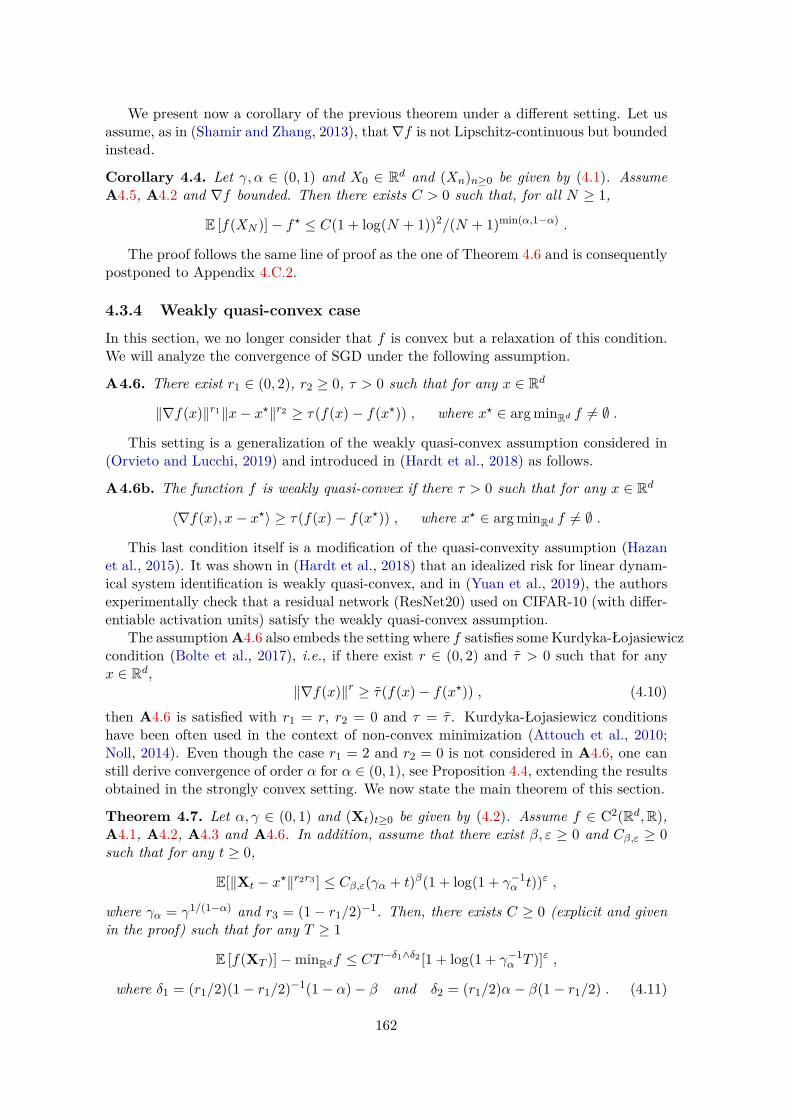
We present now a corollary of the previous theorem under a different setting. Let usassume, as in (Shamir and Zhang, 2013), that∇f is not Lipschitz-continuous but boundedinstead.

Corollary 4.4. Let γ, α ∈ (0, 1) and X0 ∈ Rd and (Xn)n≥0 be given by (4.1). AssumeA4.5, A4.2 and ∇f bounded. Then there exists C > 0 such that, for all N ≥ 1,

E [f(XN )]− f? ≤ C(1 + log(N + 1))2/(N + 1)min(α,1−α) .

The proof follows the same line of proof as the one of Theorem 4.6 and is consequentlypostponed to Appendix 4.C.2.

4.3.4 Weakly quasi-convex case

In this section, we no longer consider that f is convex but a relaxation of this condition.We will analyze the convergence of SGD under the following assumption.

A4.6. There exist r1 ∈ (0, 2), r2 ≥ 0, τ > 0 such that for any x ∈ Rd

‖∇f(x)‖r1‖x− x?‖r2 ≥ τ(f(x)− f(x?)) , where x? ∈ arg minRd f 6= ∅ .

This setting is a generalization of the weakly quasi-convex assumption considered in(Orvieto and Lucchi, 2019) and introduced in (Hardt et al., 2018) as follows.

A4.6b. The function f is weakly quasi-convex if there τ > 0 such that for any x ∈ Rd

〈∇f(x), x− x?〉 ≥ τ(f(x)− f(x?)) , where x? ∈ arg minRd f 6= ∅ .

This last condition itself is a modification of the quasi-convexity assumption (Hazanet al., 2015). It was shown in (Hardt et al., 2018) that an idealized risk for linear dynam-ical system identification is weakly quasi-convex, and in (Yuan et al., 2019), the authorsexperimentally check that a residual network (ResNet20) used on CIFAR-10 (with differ-entiable activation units) satisfy the weakly quasi-convex assumption.

The assumptionA4.6 also embeds the setting where f satisfies some Kurdyka-Łojasiewiczcondition (Bolte et al., 2017), i.e., if there exist r ∈ (0, 2) and τ > 0 such that for anyx ∈ Rd,

‖∇f(x)‖r ≥ τ(f(x)− f(x?)) , (4.10)then A4.6 is satisfied with r1 = r, r2 = 0 and τ = τ . Kurdyka-Łojasiewicz conditionshave been often used in the context of non-convex minimization (Attouch et al., 2010;Noll, 2014). Even though the case r1 = 2 and r2 = 0 is not considered in A4.6, one canstill derive convergence of order α for α ∈ (0, 1), see Proposition 4.4, extending the resultsobtained in the strongly convex setting. We now state the main theorem of this section.

Theorem 4.7. Let α, γ ∈ (0, 1) and (Xt)t≥0 be given by (4.2). Assume f ∈ C2(Rd,R),A4.1, A4.2, A4.3 and A4.6. In addition, assume that there exist β, ε ≥ 0 and Cβ,ε ≥ 0such that for any t ≥ 0,

E[‖Xt − x?‖r2r3 ] ≤ Cβ,ε(γα + t)β(1 + log(1 + γ−1α t))ε ,

where γα = γ1/(1−α) and r3 = (1− r1/2)−1. Then, there exists C ≥ 0 (explicit and givenin the proof) such that for any T ≥ 1

E [f(XT )]−minRdf ≤ CT−δ1∧δ2 [1 + log(1 + γ−1α T )]ε ,

where δ1 = (r1/2)(1− r1/2)−1(1− α)− β and δ2 = (r1/2)α− β(1− r1/2) . (4.11)

162

Note that if f satisfies a Kurdyka-Łojasiewicz condition of type (4.10) then A4.6 issatisfied with r1 = r and r2 = 0 and the rates in Theorem 4.7 simplify and we obtain thatδ = min((r/2)(1− r/2)−1(1−α), (r/2)α). The rate is maximized for α = (2− r/2)−1 andin this case, δ = r/(4− r). Therefore, if r → 2, then δ → 1 and we obtain at the limit thesame convergence rate that the case where f is strongly convex A4.4.

Proof. Without loss of generality, we assume that f? = 0. Let α, γ ∈ (0, 1), x0 ∈ Rd,at = γα + t, `t = 1 + log(1 + γ−1

α t) for any t ≥ 0 and δ = min(δ1, δ2) with δ1 and δ2 given inTheorem 4.7. Using Lemma 4.13, we have for any t ≥ 0

E[f(Xt)aδt `−εt

]− f(X0)γδα =

∫ t

0

−`−εs aδ−αs E[‖∇f(Xs)‖2] +(γα/2)`−εs aδ−2α

s E[〈∇2f(Xs),Σ(Xs)〉

]+δ`−εs aδ−1

s E [f(Xs)]− ε`−ε−1s aδsE [f(Xs)]

ds .

Define for any t ≥ 0, E(t) = E[f(Xt)]aδt `−εt . (t 7→ E(t)) is differentiable and using A4.1 andA4.2 we have for any t > 0,

dE(t)/ dt ≤ −`−εt aδ−αt E[‖∇f(Xt)‖2

]+ (γα/2)`−εt aδ−2α

t Lη + δa−1t E(t) .

Using, A4.6 and Hölder’s inequality we have for any t ≥ 0

τE [f(Xt)] ≤ E [‖Xt − x?‖r2r3 ]r−13 E[‖∇f(Xt)‖2]r1/2 .

Noting that (r3r1)−1 = r−11 − 1/2, we get for any t ≥ 0

E[‖∇f(Xt)‖2] ≥ τ2r−11 E [f(Xt)]2r

−11 E [‖Xt − x?‖r2r3 ]1−2r−1

1

≥ τ2r−11 C

1−2r−11

β,ε aβ(1−2r−1

1 )t `

ε(1−2r−11 )

t E [f(Xt)]2r−11

≥ τ2r−11 C

1−2r−11

β,ε aβ(1−2r−1

1 )−2r−11 δ

t `ε(1−2r−1

1 )−2r−11 −ε

t E(t)2r−11 .

Therefore, we have for any t ≥ 0

dE(t)/ dt ≤ −τ2r−11 C

1−2r−11

β,ε a(1−2r−1

1 )(δ+β)−αt E(t)2r−1

1 + γα`−εt aδ−2α

t Lη + δa−1t E(t) .

Let D3 = max(D1, D2) with

D1 = (|δ|C2r−11 −1

β,ε τ−2r−11 γ

(2r−11 −1)(δ+β)+α−1

α )(2r−11 −1)−1

,

D2 = ((Lη/2)C2r−11 −1

β,ε τ−2r−11 γ

(2r−11 −1)(δ+β)+δ−α+1

α )r1/2 .

If E(t) ≥ D3 then dE(t)/ dt ≤ 0. Let C = max(D3, E(0)), then for any t ≥ 0, E(t) ≤ C, whichconcludes the proof.

In the general case r2 6= 0, the convergence rates obtained in Theorem 4.7 depend onβ where (E[‖Xt − x?‖r2r3 ](γα + t)−β)t≥0 has at most logarithmic growth. If β 6= 0, thenthe convergence rates deteriorate. In what follows, we shall consider different scenariosunder which β can be explicitly controlled. These estimates imply explicit convergencerates for SGD using Theorem 4.7.

Corollary 4.5. Let α, γ ∈ (0, 1) and (Xt)t≥0 given by (4.2). Assume f ∈ C2(Rd,R),A4.1, A4.2 and A4.3.(a) If A4.6b holds, then there exists C ≥ 0 such that for any T ≥ 1

E [f(XT )]−minRdf ≤ C[T (1−3α)/2 + T−α/2 + Tα−1] .

163

(b) If A4.6b holds and there exist c,R > 0 such that for any x ∈ Rd with ‖x− x?‖ ≥ R,f(x)− f(x?) ≥ c‖x− x?‖ then there exists C ≥ 0 such that for any T ≥ 1

E [f(XT )]−minRdf ≤ C[T−α/2 + Tα−1] . (4.12)

(c) If A4.6 holds and if there exists R ≥ 0 such that for any x ∈ Rd with ‖x‖ ≥ R,〈∇f(x), x − x?〉 ≥ m ‖x− x?‖2, then there exists C ≥ 0 such that for any T ≥ 1, (4.12)holds.

The proof is postponed to Appendix 4.D. The main ingredient of the proof is to controlthe growth of t 7→ E[‖Xt− x?‖2] using either the SDE satisfied by (‖Xt− x?‖2)t≥0 in thecase of (a) and (c), or the SDE satisfied by (f(Xt)−minRdf)t≥0 in the case of (b).

Under A4.6b, we compare the rates we obtain using Corollary 4.5-(a) with the onesderived by (Orvieto and Lucchi, 2019) in Table 4.2 and Figure 4.3b. Note that comparedto (Orvieto and Lucchi, 2019), we establish that SGD converges as soon as α > 1/3 andnot α > 1/2. In addition, the convergence rates we obtain are always better than theones of (Orvieto and Lucchi, 2019) in the case α > 1/2. However, note that in both cases,the optimal convergence rate is 1/3 obtained using α = 2/3. Finally, under additionalgrowth conditions on the function f , and using Corollary 4.5-(b)-(c) we show that theconvergence of SGD in the weak quasi-convex case occurs as soon as α > 0.

Table 4.2 – Rates for continuous SGD with non-convex assumptions

Reference Corollary 4.5-(a) Corollary 4.5-(b) (OL’19)α ∈ (0, 1/3) × α/2 ×α ∈ (1/3, 1/2) (3α− 1)/2 α/2 ×

α = 1/2 1/4 + log. 1/4 + log. ×α ∈ (1/2, 2/3) α/2 1− α 2α− 1α ∈ (2/3, 1) 1− α 1− α 1− α

As in the previous sections, we extend our results to the discrete setting.

Theorem 4.8. Let α, γ ∈ (0, 1) and (Xn)n∈N be given by (4.1). Assume A4.1, A4.2and A4.6. In addition, assume that there exist β, ε, Cβ,ε ≥ 0 such that for any n ∈ N,E [‖Xn − x?‖r2r3 ] ≤ Cβ,ε(n+ 1)β1 + log(1 + n)ε, where r3 = (1− r1/2)−1. Then, thereexists C ≥ 0 (explicit and given in the proof) such that for any N ≥ 1

E [f(XN )]−minRdf ≤ CN−δ1∧δ2 (1 + log(1 +N)))ε ,

where δ1, δ2 are given in (4.11).

Proof. Without loss of generality, we assume that f? = 0. Let α, γ ∈ (0, 1), x0 ∈ Rd. Letδ = min(δ1, δ2), with δ1, δ2 given in Theorem 4.8 and let (Ek)k∈N such that for any k ∈ N,Ek = (k + 1)δE [f(Xk)] (1 + log(k + 1))−ε. There exists cδ ∈ R such that for any x ∈ [0, 1],(1 + x)δ ≤ 1 + cδx. Hence, for any n ∈ N we have

(n+ 2)δ − (n+ 1)δ ≤ (n+ 1)δ

(1 + (n+ 1)−1)δ − 1≤ cδ(n+ 1)δ−1 . (4.13)

Using (Nesterov, 2004, Lemma 1.2.3) and A4.2 we have for any n ∈ N such that n ≥ (2Lγ)1/α

E [f(Xn+1)|Fn] ≤ f(Xn)− γ(n+ 1)−αE [〈∇f(Xn), H(Xn, Zn+1)〉|Fn] (4.14)

+ (L/2)γ2(n+ 1)−2αE[‖H(Xn, Zn+1)‖2

∣∣∣Fn]164

E [f(Xn+1)] ≤ E [f(Xn)]− γ(n+ 1)−αE[‖∇f(Xn)‖2

]+ Lγ2(n+ 1)−2αE

[‖∇f(Xn)‖2

]+ Lγ2(n+ 1)−2αη

≤ E [f(Xn)]− γ(n+ 1)−α

1− Lγ(n+ 1)−αE[‖∇f(Xn)‖2

]+ Lγ2(n+ 1)−2αη

≤ E [f(Xn)]− γ(n+ 1)−αE[‖∇f(Xn)‖2

]/2 + Lγ2(n+ 1)−2αη .

Combining (4.13) and (4.14) we get for any n ∈ N such that n ≥ (2Lγ)1/2

En+1 − En = (n+ 2)δE [f(Xn+1)] (1 + log(n+ 2))−ε − (n+ 1)δE [f(Xn)] (1 + log(n+ 1))−ε(4.15)≤ (1 + log(n+ 1))−ε

[(n+ 2)δ − (n+ 1)δ

(E [f(Xn+1)])

+(n+ 1)δ E [f(Xn+1)]− E [f(Xn)]]

≤ (1 + log(n+ 1))−ε[

(n+ 2)δ − (n+ 1)δ

(E [f(Xn)] + Lγ2(n+ 1)−2αη)

+(n+ 1)δ−γ(n+ 1)−αE

[‖∇f(Xn)‖2

]/2 + Lγ2(n+ 1)−2αη

]≤ (1 + log(n+ 1))−ε

[cδ(n+ 1)δ−1(E [f(Xn)] + 2γ2(n+ 1)−2αη)

+(n+ 1)δ−γ(n+ 1)−αE

[‖∇f(Xn)‖2

]/2 + Lγ2(n+ 1)−2αη

]≤ cδEn + 2Lγ2(1 + cδ)(n+ 1)δ−2α(1 + log(n+ 1))−εη− γ(n+ 1)δ−α(1 + log(n+ 1))−εE

[‖∇f(Xn)‖2

]/2 .

Using (4.6) and the fact that for any k ∈ N, E [‖Xk − x?‖r2r3 ] ≤ Cβ,ε(k+ 1)β(1 + log(1 +k))εand Hölder’s inequality and that r1r3 = 2(2r−1

1 − 1)−1, we have for any k ∈ N

E[‖∇f(Xk)‖2

]≥ E [f(Xk)]2r

−11 C

−(2r−11 −1)−1

β,ε τ2r−11 (k+1)−β(2r−1

1 −1)(1+log(k+1))−ε(2r−11 −1) .

(4.16)Combining (4.15) and (4.16) we get that for any n ∈ N with n ≥ (4γ)1/α

En+1 − En ≤ cδEn + 2Lγ2(1 + cδ)(n+ 1)δ−2α(1 + log(n+ 1))−εη

− γ(n+ 1)δ−α−β(2r−11 −1)E [f(Xn)]2r

−11 C

−(2r−11 −1)−1

β,ε τ2r−11 (1 + log(n+ 1))−ε2r

−11 /2

≤ cδEn + 2Lγ2(1 + cδ)(n+ 1)δ−2α(1 + log(n+ 1))−εη

− γ(n+ 1)α−(δ+β)(2r−11 −1)E

2r−11

n C−(2r−1

1 −1)−1

β,ε τ2r−11 /2 .

Let D3 = max(D1, D2) with D1 = (2|cδ|C2r−1

1 −1β,ε τ−2r−1

1 )2r−11 −1 ,

D2 = (4Lγ2(1 + cδ)C2r−1

1 −1β,ε τ−2r−1

1 )r1/2 .

If En ≥ D3 and n ≥ (4γ)1/α then En+1 ≤ En. Therefore, we obtain by recursion that En ≤ Cwith C = max(E0, . . . , Ed(2Lγ)1/αe, D3).

We can conduct the same discussion as the one after Theorem 4.7 and Corollary 4.5can be extended to the discrete case.

Corollary 4.6. Let α, γ ∈ (0, 1) and x0 ∈ Rd. Assume A4.1, A4.2. Then we have:

(a) if A4.6b holds then, there exists C ≥ 0 such that for any N ∈ N?

E [f(XN )]− f? ≤ C[N (1−3α)/2 +N−α/2 +Nα−1

],

165

(b) if A4.6 holds and if there exists R ≥ 0 such that for any x ∈ Rd with ‖x‖ ≥ R,〈∇f(x), x− x?〉 ≥ m ‖x− x?‖2, then there exists C ≥ 0 such that for any N ∈ N?

E [f(XN )]− f? ≤ C[N−α/2 +Nα−1

].

Proof. Let α, γ ∈ (0, 1) and x0 ∈ Rd. We have for any n ∈ N,

E[‖Xn+1 − x?‖2

]= E

[‖Xn − x?‖2

]+ 2E [〈Xn − x?, Xn+1 −Xn〉] + E

[‖Xn+1 −Xn‖2

](4.17)

≤ E[‖Xn − x?‖2

]− 2γ(n+ 1)−αE [〈Xn − x?,∇f(Xn)〉]

+ 2γ2(n+ 1)−2αE[‖∇f(Xn)‖2

]+ 2γ(n+ 1)−2αη .

We now divide the proof into two parts.(a) Using A4.6b and Lemma 4.16 we have for any x ∈ Rd,

〈∇f(x), x− x?〉 ≥ τ(f(x)− f(x?)) ≥ τ ‖∇f(x)‖2 /(2L) . (4.18)

Using A4.1, (4.17) and (4.18) we have for any n ≥ (4γL/τ)1/α

E[‖Xn+1 − x?‖2

]≤ E

[‖Xn − x?‖2

]+ 2γ(n+ 1)−α(−τ/(2L) + γ(n+ 1)−α)E

[‖∇f(Xn)‖2

]+ 2γ(n+ 1)−2αη

≤ E[‖Xn − x?‖2

]+ 2γ(n+ 1)−2αη .

Therefore, there exist β, ε ≥ 0 and Cβ,ε ≥ 0 such that E[‖Xn − x?‖2] < Cβ,ε(n + 1)−β(1 +log(1 +n))ε with β = 0 and ε = 0 if α > 1/2, β = 1− 2α and ε = 0 if α < 1/2 and β = 0 andε = 1 if α = 1/2. Combining this result and Theorem 4.8 concludes the proof.(b) Finally, assume that there exists R ≥ 0 such that for any x ∈ Rd with ‖x‖ ≥ R,〈∇f(x), x − x?〉 ≥ m ‖x− x?‖2. Therefore, since (x 7→ ∇f(x)) is continuous, there existsa ≥ 0 such that for any x ∈ Rd, 〈∇f(x), x − x?〉 ≥ m ‖x− x?‖2 − a. Combining this resultand (4.17) we get that for any n ∈ N such that n ≥ (2/γ)α−1

E[‖Xn+1 − x?‖2

]≤ (1− γ(n+ 1)−α)E

[‖Xn − x?‖2

]+ 2γ(n+ 1)−αa + 2γ2(n+ 1)−2αη .

Hence, if n ≥ (2/γ)−α−1 and E[‖Xn−x?‖2] ≥ max(2a, 2γη) then E[‖Xn+1−x?‖2] ≤ E[‖Xn−x?‖2]. Therefore, we obtain by recursion that for any n ∈ N, that (E[‖Xn − x?‖2])n∈N isbounded which concludes the proof by applying Theorem 4.8.

166

0 1/3 1/2 2/3 1

1/41/3

1/2

1

α

rate

ofconv

ergence

strongly convex deterministicconvex (Thm 4.6) (Bach and Moulines, 2011, Table 1)

(a) Convex setting : comparison with (Bachand Moulines, 2011)

0 1/3 1/2 2/3 1

1/41/3

1/2

1

α

rate

ofconv

ergence

strongly convex deterministicCor.4.5-(a) Cor.4.5-(b)

(Orvieto and Lucchi, 2019, Table 1)

(b) Weakly quasi-convex setting : comparisonwith (Orvieto and Lucchi, 2019)

Figure 4.3 – Comparison of the convergence rates in the convex and weakly quasi-convexsettings.

4.4 ConclusionIn this chapter we investigated the connection of SGD with solutions of a particulartime inhomogenuous SDE. We first proved approximation bounds between these twoprocesses motivating convergence analysis of continuous SGD. Then, we turned to theconvergence behavior of SGD and showed how the continuous process can provide a betterunderstanding of SGD using tools from ODE and stochastic calculus. In particular, weobtained optimal convergence rates in the strongly convex and convex cases. In thenon-convex setting, we considered a relaxation of the weakly quasi-convex condition andimproved the state-of-the art convergence rates in both the continuous and discrete-timesetting.

4.A Proofs of the approximation resultsIn this section2, we present the proof of Proposition 4.1 in Appendix 4.A.3 and the oneof Proposition 4.2 in Appendix 4.A.4. We begin this section by some useful technicallemmas and results on moment bounds. Throughout this section we will denote all theconstants by the letter A followed by some subscript.

4.A.1 Technical Lemmas

The following lemma is well-known but is recalled as well as its proof for completeness

Lemma 4.4. Let f ∈ C1(Rd,R). Assume that there exists L ≥ 0 such that for anyx, y ∈ Rd, ∇f is L-Lipschitz and that f admits a minimum. Then for any x ∈ Rd

‖∇f(x)‖2 ≤ (L/2)(f(x)−min f) . (4.19)

Proof. Using (Nesterov, 2004, Lemma 1.2.3), we have for any x, y ∈ Rd

f(y)− f(x) ≤ 〈∇f(x), y − x〉+ (L/2) ‖y − x‖2 .

We obtain (4.19) by minimizing both side of the previous inequality.2This section is mainly the work of Valentin De Bortoli, but is put here for completeness.

167

Lemma 4.5. Let (un)n∈N, (vn)n∈N and (wn)n∈N such that for any n ∈ N, un, vn, wn ≥ 0,u0 ≥ 0 and un+1 ≤ (1 + vn)un + wn. Then for any n ∈ N

un ≤ exp[n−1∑k=0

vk

](u0 +

n−1∑k=0

wk

).

Proof. The proof is a straightforward consequence of the discrete Grönwall’s lemma.

Lemma 4.6. Let r > 0, γ > 0 and α ∈ [0, 1). Then for any T ≥ 0, there exists Aα,r ≥ 0such that for any N ∈ N with Nγα ≤ T we have

γrN−1∑k=0

(k + 1)−αr ≤

Aα,rγr(1 + log(γ−1))(1 + log(T )) , if α ≥ 1/r ,Aα,rγrγαr−1

α T 1−αr otherwise .

Note that if r = 1 then γr∑N−1k=0 (k+1)−αr ≤ Aα,1T 1−α. Using a slight modification of

Lemma 4.6 we also obtain that there exists A such that if r = 1 then γr∑N−1k=0 (k+1)−αr ≤

T 1−α + A.

Proof. Let r > 0, γ > 0 and α ∈ [0, 1). If α > 1/r then there exists Aα,r ≥ 0 such that

γrN−1∑k=0

(k + 1)−αr ≤ Aα,rγr .

If α < 1/r then there exists Aα,r ≥ 0 such that

γrN−1∑k=0

(k + 1)−αr ≤ Aα,rγrN−αr+1 ≤ Aα,rγrγαr−1α T 1−αr .

if α = 1/r then there exists Aα,r ≥ 0 such that

γrN−1∑k=0

(k + 1)−αr ≤ γr(1 + log(N)) ≤ Aα,rγr(1 + log(T ))(1 + log(γ−1)) .

4.A.2 Moment bounds

The following result is well-known in the field of SDE but its proof is given for complete-ness.

Lemma 4.7. Let p ∈ N, γ > 0 and α ∈ [0, 1). Assume A4.1 and A4.2. Then for anyT ≥ 0, there exists AT,1 ≥ 0, such that for any s ≥ 0 and t ∈ [s, s+ T ], γ ∈ (0, γ] andX0 ∈ Rd, we have

E[1 + ‖Xt‖2p

]≤ AT,1(1 + ‖X0‖2p) ,

where (Xt)t≥0 is the solution of (4.2) such that Xs = X0.If in addition, for any x ∈ Rd, µZ(‖H(x, ·)−∇f(x)‖2p) ≤ ηp, with ηp ≥ 0, then for any

T ≥ 0, there exists AT,1 ≥ 0, such that for any k0 ≥ 0, γ ∈ (0, γ] and k ∈ k0, . . . , k0 +Nwith Nγα ≤ T , and X0 ∈ Rd, we have

E[1 + ‖Xk‖2p

]≤ AT,1(1 + ‖X0‖2p) ,

where (Xk)k∈N satisfies the recursion (4.1) with Xk0 = X0

168

Proof. Let p ∈ N, α ∈ [0, 1), s, T ∈ [0,+∞), t ∈ [s, s+ T ], X0 ∈ Rd and gp ∈ C2(Rd, [0,+∞))such that for any x ∈ Rd, gp(x) = 1 + ‖x‖2p. Let γ > 0 and γ ∈ (0, γ].

We divide the proof into two parts(a) Let (Xt)t≥0 be a solution to (4.2) such that Xs = X0. We have for any x ∈ Rd

∇gp(x) = 2p ‖x‖2(p−1)x , ∇2gp(x) = 4p(p− 1) ‖x‖2(p−2)

xx>

+ 2p ‖x‖2(p−1) Id . (4.20)

Let n ∈ N, and set τn = infu ≥ 0 : gp(Xu) > n. Applying Itô’s lemma and using (4.2)and (4.20) we get

E [gp(Xt∧τn)]− E [gp(Xs∧τn)] = E[∫ t∧τn

s∧τn−(γα + u)−α〈∇f(Xu),∇gp(Xu)〉

]du (4.21)

+ (γα/2)E[∫ t∧τn

s∧τn(γα + u)−2α〈Σ(Xu),∇2gp(Xu)〉du

].

Using A4.1, (4.20) and the Cauchy-Schwarz inequality we get that for any u ∈ [s, s+ T ]

|〈∇f(Xu),∇gp(Xu)〉| ≤ 2p‖Xu‖2(p−1) |〈∇f(Xu)−∇f(0),Xu〉|+ ‖∇f(0)‖‖Xu‖(4.22)≤ 2p(L + ‖∇f(0)‖)gp(Xu) .

In addition, using A4.1, A4.2, (4.20) and the Cauchy-Schwarz inequality we get that for anyu ∈ [s, s+ T ]

〈Σ(Xu),∇2gp(Xu)〉 = 2p ‖Xu‖2(p−1)∫

Z‖∇f(Xu)−H(Xu, z)‖2 dµZ(z)

+ 4p(p− 1) ‖Xu‖2(p−2)∫

Z〈Xu, H(Xu, z)−∇f(Xu)〉2dµZ(z)

≤ 2p(2p− 1) ‖Xu‖2(p−1)η ≤ 2p(2p− 1)ηgp(Xu) . (4.23)

Combining (4.22) and (4.23) in (4.21) we get for large enough n ∈ N

E [gp(Xt∧τn)]− gp(X0) ≤ 2p(L + ‖∇f(0)‖)E[∫ t∧τn

s

gp(Xu)du]

+ γαp(2p− 1)E[∫ t∧τn

s

gp(Xu)du]

≤ 2p(L + ‖∇f(0)‖) + γαp(2p− 1)∫ t

s

E [gp(X∧τn)] du .

Using Grönwall’s lemma we obtain

E [gp(Xt∧τn)] ≤ gp(X0) exp [T 2p(L + ‖∇f(0)‖) + γαp(2p− 1)] .

We conclude upon using Fatou’s lemma and remarking that limn τn = +∞, since Xt iswell-defined for any t ≥ 0.(b) Let (Xk)k∈N be a sequence which satisfies the recursion (4.1) with Xk0 = X0. LetAk = Xk − γ(k + 1)−α∇f(Xk) and Bk = γ(k + 1)−α(∇f(Xk) − H(Xk, Zk+1)). We have,using Cauchy-Schwarz inequality and the binomial formula,

‖Xk+1‖2p = ‖Ak +Bk‖2p =‖Ak‖2 + 2〈Ak, Bk〉+ ‖Bk‖2

p≤

p∑i=0

i∑j=0

(p

i

)(i

j

)‖Ak‖2(p−i)+j ‖Bk‖2i−j × 2j

≤ ‖Ak‖2p + 2pp∑i=1

i∑j=0

(p

i

)(i

j

)‖Ak‖2(p−i)+j ‖Bk‖2i−j . (4.24)

169

Using A4.1, there exists A(a)T,1, A

(b)T,1, A

(c)T,1 ≥ 0 such that for any ` ∈ 0, . . . , 2p

‖Ak‖` ≤∑m=0

(`

m

)(1 + γ(k + 1)−αL)m ‖Xk‖m

(γ(k + 1)−α ‖∇f(0)‖

)`−m≤ (1 + γ(k + 1)−αA(a)

T,1) ‖Xk‖` + γ(k + 1)−αA(b)T,1(1 + ‖Xk‖2p)

≤ (1 + γ(k + 1)−αA(c)T,1)(1 + ‖Xk‖2p) .

Combining this result, (4.24), Jensen’s inequality and that for any ` ∈ N, E[‖Bk‖2`

∣∣Fk] ≤γ2`(k + 1)−2α`η` we have

E[‖Xk+1‖2p

∣∣Fk] ≤ (1 + γ(k + 1)−αA(a)T,1) ‖Xk‖` + γ(k + 1)−αA(b)

T,1(1 + ‖Xk‖2p)

+ 2p(1 + γ(k + 1)−αA(c)T,1)(1 + ‖Xk‖2p)

p∑i=1

i∑j=0

(p

i

)(i

j

)η

1/22i−jγ

2i−j(k + 1)−α(2i−j) .

Therefore, there exists A(d)T,1 ≥ 0 such that

E[1 + ‖Xk+1‖2p

]≤ (1 + A(d)

T,1γ(k + 1)−α)E[1 + ‖Xk‖2p

]+ A(d)

T,1γ(k + 1)−α .

We conclude combining this result, Lemma 4.5 and Lemma 4.6.

We use the previous result to prove the following lemma.

Lemma 4.8. Let p ∈ N, γ > 0 and α ∈ [0, 1). Assume A4.1, A4.2 and that for anyx ∈ Rd, µZ(‖H(x, ·) − ∇f(x)‖2p) ≤ ηp, with ηp ≥ 0. Then for any T ≥ 0, there existsAT,2 ≥ 0 such that for any γ ∈ (0, γ], k ∈ N with (k + 1)γα ≤ T , t ∈ [kγα, (k + 1)γα] andX0 ∈ Rd, we have

maxE[‖Xk+1 −X0‖2p

],E[‖Xt −X0‖2p

]≤ AT,2(k + 1)−2αpγ2p(1 + ‖X0‖2p) ,

where (Xk)k∈N satisfies the recursion (4.1) with Xk = X0 and (Xt)t≥0 is the solution of(4.2) with Xkγα = X0.

Proof. Let p ∈ N, α ∈ [0, 1), γ > 0, γ ∈ (0, γ], k ∈ N, t ∈ [kγα, (k + 1)γα] and X0 ∈ Rd. Wedivide the rest of the proof into two parts.(a) Let (Xt)t≥0 be a solution to (4.2) such that Xkγα = X0. Using A4.1, A4.2, Jensen’sinequality, Burkholder-Davis-Gundy’s inequality (Rogers and Williams, 2000, Theorem 42.1)and Lemma 4.7 there exists Bp ≥ 0 such that

E[‖Xt −X0‖2p

]≤ 22p−1E

[∥∥∥∥∫ t

kγα

(γα + s)−α∇f(Xs)ds∥∥∥∥2p]

+ 22p−1γpαE

[∥∥∥∥∫ t

kγα

(γα + s)−αΣ(Xs)1/2dBs

∥∥∥∥2p]

≤ 22p−1γ2p−1α

∫ t

kγα

(γα + s)−2αpE[‖∇f(Xs)‖2p

]ds

+Bp22p−1γpα

(∫ t

kγα

(γα + s)−2αE [Tr(Σ(Xs))] ds)p

≤ 22p−1γ2p−1−2αpα (k + 1)−2αp(Bp + 1)

∫ t

kγα

E[‖∇f(Xs)‖2p

]ds

170

+∫ t

kγα

E [Tr(Σ(Xs))]p ds

≤ 24p−2(1 + L2p)γ2pγ−1α (k + 1)−2αp(Bp + 1)

∫ t

kγα

‖∇f(0)‖2p ds

+∫ t

kγα

(E[‖Xs‖2p

]+ ηp

)ds

≤ 24p−2(1 + L2p)γ2p(k + 1)−2αp(Bp + 1)‖∇f(0)‖2p

+ηp + sups∈[kγα,t]

E[‖Xs‖2p

]≤ 24p−2(1 + L2p)γ2p(k + 1)−2αp(Bp + 1)

(‖∇f(0)‖2p + ηp + AT,1

)gp(X0) .

(4.25)

(b) Let (Xn)n∈N satisfying the recursion (4.1) with Xk = X0. Using A4.1 and A4.2 we getthat

E[‖Xk+1 −X0‖2p

]= E

[∥∥−γ(k + 1)−α(∇f(X0) +H(X0, Zk+1)−∇f(X0))∥∥2p]

≤ γ2p(k + 1)−2αp32p−1(

L2p ‖∇f(0)‖2p + L2p ‖X0‖2p

+∫

Z‖H(X0, z)−∇f(X0)‖2p dµZ(z)

)≤ γ2p(k + 1)−2αp32p−1(1 + L2p)

(1 + ‖∇f(0)‖2p + ηp

)(1 + ‖X0‖2p) .

(4.26)

Combining (4.25) and (4.26) and setting

AT,2 = 24p−2(1 + L2p)(‖∇f(0)‖2p + ηp + max(AT,1, 1)

),

conclude the proof upon remarking that ηp ≤ ηp.

4.A.3 Mean-square approximation

Now consider the stochastic process (Xt)t≥0 defined by X0 = X0 and solution of thefollowing SDE

dXt = −γ−1α

+∞∑k=0

1[kγα,(k+1)γα)(t)(1 + k)−αγ∇f(Xkγα)dt+ γ1/2

α Σ(Xkγα)1/2dBt

.

(4.27)Note that for any k ∈ N, we have

X(k+1)γα = Xkγα − γ(k + 1)−α∇f(Xkγα) + Σ(Xkγα)1/2Gk

,

with Gk = γ−1/2α

∫ (k+1)γαkγα

dBs. Hence, for any k ∈ N, Xkγα has the same distribution asXk given by (4.1) with H(x, z) = ∇f(x) + Σ(x)1/2z, (Z,Z) = (Rd,B(Rd)) and µZ theGaussian probability distribution with zero mean and covariance matrix identity.Lemma 4.9. Let γ > 0 and α ∈ [0, 1). Assume A4.2. Then for any T ≥ 0, there existsAT,3 ≥ 0 such that for any γ ∈ (0, γ], k ∈ N with (k + 1)γα ≤ T and X0 ∈ Rd we have

E[‖X(k+1)γα −Xk+1‖2

]≤ AT,3γ2(k + 1)−2α(1 + ‖X0‖2) ,

where (Xk)k∈N satisfies the recursion (4.1) with Xk = X0 and (Xt)t≥0 is the solution of(4.27) with Xkγα = X0.

171

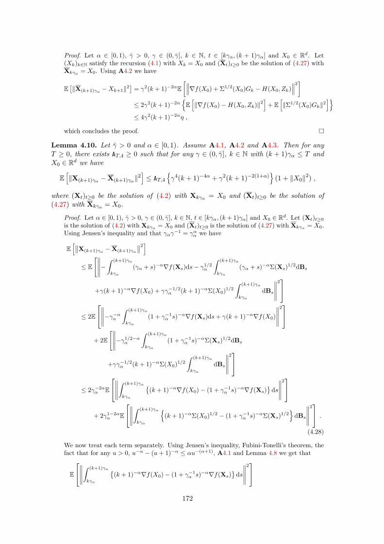
Proof. Let α ∈ [0, 1), γ > 0, γ ∈ (0, γ], k ∈ N, t ∈ [kγα, (k + 1)γα] and X0 ∈ Rd. Let(Xk)k∈N satisfy the recursion (4.1) with Xk = X0 and (Xt)t≥0 be the solution of (4.27) withXkγα = X0. Using A4.2 we have

E[‖X(k+1)γα −Xk+1‖2

]= γ2(k + 1)−2αE

[∥∥∥∇f(X0) + Σ1/2(X0)Gk −H(X0, Zk)∥∥∥2]

≤ 2γ2(k + 1)−2αE[‖∇f(X0)−H(X0, Zk)‖2

]+ E

[‖Σ1/2(X0)Gk‖2

]≤ 4γ2(k + 1)−2αη ,

which concludes the proof.

Lemma 4.10. Let γ > 0 and α ∈ [0, 1). Assume A4.1, A4.2 and A4.3. Then for anyT ≥ 0, there exists AT,4 ≥ 0 such that for any γ ∈ (0, γ], k ∈ N with (k + 1)γα ≤ T andX0 ∈ Rd we have

E[‖X(k+1)γα −X(k+1)γα‖

2]≤ AT,4

γ4(k + 1)−4α + γ2(k + 1)−2(1+α)

(1 + ‖X0‖2) ,

where (Xt)t≥0 be the solution of (4.2) with Xkγα = X0 and (Xt)t≥0 be the solution of(4.27) with Xkγα = X0.

Proof. Let α ∈ [0, 1), γ > 0, γ ∈ (0, γ], k ∈ N, t ∈ [kγα, (k + 1)γα] and X0 ∈ Rd. Let (Xt)t≥0is the solution of (4.2) with Xkγα = X0 and (Xt)t≥0 is the solution of (4.27) with Xkγα = X0.Using Jensen’s inequality and that γαγ−1 = γαα we have

E[∥∥X(k+1)γα −X(k+1)γα

∥∥2]≤ E

[∥∥∥∥∥−∫ (k+1)γα

kγα

(γα + s)−α∇f(Xs)ds− γ1/2α

∫ (k+1)γα

kγα

(γα + s)−αΣ(Xs)1/2dBs

+γ(k + 1)−α∇f(X0) + γγ−1/2α (k + 1)−αΣ(X0)1/2

∫ (k+1)γα

kγα

dBs

∥∥∥∥∥2

≤ 2E

∥∥∥∥∥−γ−αα∫ (k+1)γα

kγα

(1 + γ−1α s)−α∇f(Xs)ds+ γ(k + 1)−α∇f(X0)

∥∥∥∥∥2

+ 2E[∥∥∥∥∥−γ1/2−α

α

∫ (k+1)γα

kγα

(1 + γ−1α s)−αΣ(Xs)1/2dBs

+γγ−1/2α (k + 1)−αΣ(X0)1/2

∫ (k+1)γα

kγα

dBs

∥∥∥∥∥2

≤ 2γ−2αα E

∥∥∥∥∥∫ (k+1)γα

kγα

(k + 1)−α∇f(X0)− (1 + γ−1

α s)−α∇f(Xs)

ds∥∥∥∥∥

2

+ 2γ1−2αα E

∥∥∥∥∥∫ (k+1)γα

kγα

(k + 1)−αΣ(X0)1/2 − (1 + γ−1

α s)−αΣ(Xs)1/2

dBs

∥∥∥∥∥2 .

(4.28)

We now treat each term separately. Using Jensen’s inequality, Fubini-Tonelli’s theorem, thefact that for any u > 0, u−α − (u+ 1)−α ≤ αu−(α+1), A4.1 and Lemma 4.8 we get that

E

∥∥∥∥∥∫ (k+1)γα

kγα

(k + 1)−α∇f(X0)− (1 + γ−1

α s)−α∇f(Xs)

ds∥∥∥∥∥

2

172

≤ γ2α sups∈[kγα,(k+1)γα]

E[∥∥(k + 1)−α∇f(X0)− (1 + γ−1

α s)−α∇f(Xs)∥∥2]

ds

≤ 2γ2α sups∈[kγα,(k+1)γα]

‖∇f(X0)‖2|(k + 1)−α − (1 + γ−1

α s)−α|2

+(1 + γαs−1)−2αE

[‖∇f(Xs)−∇f(X0)‖2

]≤ 2γ2

α

[α2‖∇f(X0)‖2(k + 1)−2(1+α) + (k + 1)−2αL2 sup

s∈[kγα,(k+1)γα]E[‖Xs −X0‖2

]]≤ 2γ2

α

[α2‖∇f(X0)‖2(k + 1)−2(1+α) + (k + 1)−4αL2AT,2γ2(1 + ‖X0‖2)

]≤ 2γ2

α

[α2(‖∇f(0)‖2 + L2)(k + 1)−2(1+α) + (k + 1)−4αL2AT,2γ2

](1 + ‖X0‖2) . (4.29)

In addition, using Jensen’s inequality, Itô isometry, Fubini-Tonelli’s theorem, A4.1, A4.3and Lemma 4.8 we have

E

∥∥∥∥∥∫ (k+1)γα

kγα

(k + 1)−αΣ(X0)1/2 − (1 + γ−1

α s)−αΣ(Xs)1/2

dBs

∥∥∥∥∥2

≤ 2[

(k + 1)−2α|∫ (k+1)γα

kγα

E[‖Σ(X0)1/2 − Σ(Xs)1/2‖2

]ds|

+η|∫ (k+1)γα

kγα

(k + 1)−α − (1 + γ−1α s)2ds|

]

≤ 2γα

[(k + 1)−2αM2 sup

s∈[kγα,(k+1)γα]E[‖Xs −X0‖2

]+ ηα2(k + 1)−2(1+α)

]≤ 2γα

[(k + 1)−4αM2AT,2γ2 + ηα2(k + 1)−2(1+α)

](1 + ‖X0‖2) . (4.30)

Combining (4.28), (4.29) and (4.30) concludes the proof upon settingAT,4 = 4

[M2AT,2 + ηα2 + α2(‖∇f(0)‖2 + L2) + L2AT,2

].

Proposition 4.5. Let γ > 0 and α ∈ [0, 1). Assume A4.1, A4.2 and A4.3. Then forany T ≥ 0, there exists AT,5 ≥ 0 such that for any γ ∈ (0, γ], k ∈ N with (k + 1)γα ≤ Tand X0 ∈ Rd we have

E[‖X(k+1)γα −Xk+1‖2

]≤ AT,5

γ4(k + 1)−4α + γ2(k + 1)−2α

(1 + ‖X0‖2) ,

where (Xk)k∈N satisfies the recursion (4.1) with Xk = X0 and (Xt)t≥0 is the solution of(4.2) with Xkγα = X0.

Proof. The proof is straightforward upon combining Lemma 4.9 and Lemma 4.10.

We obtain now the following proposition which is a restatement of Proposition 4.1.Proposition 4.6. Let γ > 0 and α ∈ [0, 1). Assume A4.1, A4.2 and A4.3. Then forany T ≥ 0, there exists A1 ≥ 0 such that for any γ ∈ (0, γ], k ∈ N with kγα ≤ T we have

E1/2[‖Xkγα −Xk‖2

]≤ A1γ

δ(1 + log(γ−1)) ,

with δ = min(1, (1 − α)−1/2). If in addition, (Z,Z) = (Rd,B(Rd)) and for any x ∈ Rd,z ∈ Rd and n ∈ N,

H(x, z) = ∇f(x) + Σ(x)1/2z , Zn+1 = γ−1α

∫ (n+1)γα

nγαdBs ,

then δ = 1.

173

Proof. Let p ∈ N, α ∈ [0, 1), γ > 0, γ ∈ (0, γ], k ∈ N, and X0 ∈ Rd. Let (Ek)k∈Nsuch that for any k ∈ N, Ek = E

[‖Xkγα −Xk‖2

]. Note that E0 = 0. Let Y(k+1)γα =

Xkγα − γ(k + 1)−αH(Xkγα , Zk+1). We have

Ek+1 = E[∥∥X(k+1)γα −Xk+1

∥∥2]

= E[∥∥X(k+1)γα −Y(k+1)γα + Y(k+1)γα −Xk+1

∥∥2]

= E[∥∥X(k+1)γα −Y(k+1)γα

∥∥2]

+ 2E[〈X(k+1)γα −Y(k+1)γα ,Y(k+1)γα −Xk+1〉

]+ E

[∥∥Y(k+1)γα −Xk+1∥∥2]

= E[∥∥X(k+1)γα −Y(k+1)γα

∥∥2]

+ E[∥∥Y(k+1)γα −Xk+1

∥∥2]

+ 2E[〈X(k+1)γα −Y(k+1)γα ,Xkγα −Xk

]+ 2γ(k + 1)−αE

[〈X(k+1)γα −Y(k+1)γα , H(Xk, Zk+1)−H(Xkγα , Zk+1)〉

].(4.31)

Let ak = γ4(k + 1)−4α + γ2(k + 1)−2α. We now bound each of the four terms appearing in(4.31)(a) First, we have using Proposition 4.5 and Lemma 4.7

E[∥∥X(k+1)γα −Y(k+1)γα

∥∥2]

= E[E[∥∥X(k+1)γα −Y(k+1)γα

∥∥2∣∣∣Xkγα

]]≤ E

[AT,5(γ4(k + 1)−4α + γ2(k + 1)−2α)

(1 + ‖Xkγα‖

2)]

≤ AT,1AT,5(γ4(k + 1)−4α + γ2(k + 1)−2α)(

1 + ‖X0‖2)≤ A(a)

T,6ak ,

(4.32)

with A(a)T,6 ≥ 0 which does not depend on γ and k.

(b) Second, we have using A4.1, A4.5 and that for any a, b ≥ 0, (a+ b)2 ≤ 2a2 + 2b2

E[∥∥Y(k+1)γα −Xk+1

∥∥2]

= E[∥∥Xkγα −Xk − γ(k + 1)−α(H(Xkγα , Zk+1)−H(Xk, Zk+1))

∥∥2]

= E[∥∥Xkγα − γ(k + 1)−α∇f(Xkγα)−Xk + γ(k + 1)−α∇f(Xk)

∥∥2]

+ γ2(k + 1)−2αE [‖H(Xkγα , Zk+1)−∇f(Xkγα)

+H(Xk, Zk+1)−∇f(Xk)‖2]

≤ (1 + γL(k + 1)−α)2 ‖Xkγα −Xk‖2 + 4γ2(k + 1)−2α

≤ (1 + 2γL(k + 1)−α + γ2L2(k + 1)−2α)Ek + 4γ2(k + 1)−2α

≤ (1 + A(b)T,6a

1/2k )Ek + 4ak , (4.33)

with A(b)T,6 ≥ 0 which does not depend on γ and k.

(c) Let Y(k+1)γα = Xkγα−γ(k+1)−α∇f(Xkγα) + Σ(Xkγα)1/2Gk

, withGk = γ

−1/2α

∫ (k+1)γαkγα

dBs.Let bk = γ3(k + 1)−3α + γ(k + 1)−2(1+α/2).Using A4.2 we have E

[Y(k+1)γα

∣∣σ(Xkγα)]

= E[Y(k+1)γα

∣∣σ(Xkγα)]. Combining this result,

the Cauchy-Schwarz inequality, Lemma 4.10, Lemma 4.7 and that for any a, b ≥ 0, (a+b)1/2 ≤a1/2 + b1/2 and 2ab ≤ a2 + b2 we obtain

E[〈X(k+1)γα −Y(k+1)γα ,Xkγα −Xk〉

]= E

[〈E[X(k+1)γα −Y(k+1)γα

∣∣σ(Xkγα , Xk)],Xkγα −Xk〉

]= E

[〈E[X(k+1)γα −Y(k+1)γα

∣∣σ(Xkγα , Xk)],Xkγα −Xk〉

]174

≤ E[E1/2

[∥∥X(k+1)γα −Y(k+1)γα∥∥2∣∣∣σ(Xkγα , Xk)

]‖Xkγα −Xk‖

]≤ E1/2

[∥∥X(k+1)γα −Y(k+1)γα∥∥2]E1/2

[‖Xkγα −Xk‖2

]≤ A1/2

T,1A1/2T,4

γ4(k + 1)−4α + γ2(k + 1)−2(1+α)

1/2(1 + ‖X0‖2)E1/2

k

≤ A1/2T,1A1/2

T,4

γ3/2(k + 1)−3α/2 + γ1/2(k + 1)−(1+α/2)

(1 + ‖X0‖2)γ1/2(k + 1)−α/2E1/2

k

≤ A(c)T,6

γ3(k + 1)−3α + γ(k + 1)−2(1+α/2)

/2 + a

1/2k Ek/2 ≤ A(c)

T,6bk/2 + a1/2k Ek/2 .

(4.34)

with A(c)T,6 ≥ 0 which does not depend on γ and k.

(d) Finally, using the Cauchy-Schwarz inequality, (4.32), A4.2 and A4.1 and that for anya, b ≥ 0, (a+ b)1/2 ≤ a1/2 + b1/2, we have

γ(k + 1)−αE[〈X(k+1)γα −Y(k+1)γα , H(Xk, Zk+1)−H(Xkγα , Zk+1)〉

]≤ γ(k + 1)−αE1/2

[∥∥X(k+1)γα −Y(k+1)γα∥∥2]E1/2

[‖H(Xk, Zk+1)−H(Xkγα , Zk+1)‖2

]≤ (A(a)

T,6)1/2γ(k + 1)−αa1/2k

LE1/2

[‖Xkγα −Xk‖2

]+√

2η

≤ (A(a)T,6)1/2γ(k + 1)−αa1/2

k

√3LE1/2

[‖Xkγα −Xk‖2

]+√

6√η

≤ (A(a)T,6)1/2γ(k + 1)−αa1/2

k 2LE1/2k +

√6√η(A(a)

T,6)1/2γ(k + 1)−αa1/2k

≤ A(a)T,6γ

2(k + 1)−2αa1/2k L2 + a

1/2k Ek +

√6√η(A(a)

T,6)1/2γ(k + 1)−αa1/2k

≤ A(d)T,6

ak + a

3/2k

+ a

1/2k Ek , (4.35)

with A(d)T,6 ≥ 0 which does not depend on γ and k.

Finally, we have using (4.32), (4.33), (4.34) and (4.35) in (4.31)

Ek+1 ≤

1 + (2 + A(b)T,6)a1/2

k

Ek + (4 + A(a)

T,6 + A(d)T,6)ak + A(d)

T,6a3/2k + A(c)

T,6bk (4.36)

≤

1 + (2 + A(b)T,6)a1/2

k

Ek + (4 + A(a)

T,6 + 2A(d)T,6 + A(c)

T,6)(ak + a3/2k + bk) .

Using Lemma 4.6 and that a1/2k ≤ γ(k + 1)−α + γ2(k + 1)−2α, there exists A(e)

T,6 ≥ 0 whichdoes not depend on γ and k such that

(2 + A(b)T,6)

N−1∑k=0

a1/2k ≤ A(e)

T,6 . (4.37)

In addition, we have

ak + a3/2k + bk

≤ (1 + 23/2)[γ2(k + 1)−2α + γ3(k + 1)−3α + γ4(k + 1)−4α + γ6(k + 1)−6α + γ(k + 1)−2(1+α)

].

Therefore, using that γγαα = γα and Lemma 4.6 there exists A(f)T,6 ≥ 0 which does not depend

on γ and k such thatN−1∑k=0

(4 + A(a)T,6 + 2A(d)

T,6 + A(c)T,6)(ak + a

3/2k + bk) ≤

A(f)T,6γ

2(1 + log(γ−1)) if α ≥ 1/2 ,

A(f)T,6γα if α < 1/2 .

(4.38)

We denote vk = (2 + A(b)T,6)a1/2

k and wk = (4 + A(a)T,6 + 2A(d)

T,6 + A(c)T,6)(ak + a

3/2k + bk). Using

(4.36) and Lemma 4.5 we obtain that

Ek ≤N−1∑k=0

wk + exp[N−1∑k=0

vk

]N−1∑k=0

vkwk (4.39)

175

≤N−1∑k=0

wk + exp[N−1∑k=0

vk

](N−1∑k=0

vk

)(N−1∑k=0

wk

).

Combining (4.37), (4.38) and (4.39) concludes the first part of the proof.For the second part of the proof H(x, z) = ∇f(x) + Σ(x)1/2z and for any k ∈ N, we have

Zk+1 =∫ (k+1)γαkγα

dBs. We denote ck = γ4(k + 1)−4α + γ2(k + 1)−2(1+α). In (4.32), ak isreplaced by ck. The bound in (4.33) is replaced by (1 + A(b)

T,6a1/2k )Ek. The bound in (4.34)

remains unchanged and in (4.35) the upper-bound is replaced by A(c)T,6a

1/2k ck + a

1/2k Ek. The

rest of the proof is similar to the general case.

4.A.4 Weak approximation

We recall that Gp is the set of twice continuously differentiable functions from Rd to Rsuch that for any g ∈ Gp, there exists K ≥ 0 such that for any x ∈ Rd

max‖∇g(x)‖ ,

∥∥∥∇2g(x)∥∥∥ ≤ K(1 + ‖x‖p) , (4.40)

with p ∈ N.The following lemma will be useful.

Lemma 4.11. Let p ∈ N, g ∈ Gp and let K ≥ 0 as in (4.40). Then, for any x, y ∈ Rd

|g(y)− g(x)− 〈∇g(x), y − x〉| ≤ K(1 + ‖x‖p + ‖y‖p) ‖x− y‖2 .

Proof. Using that for any x 7→ ‖x‖p is convex, and Cauchy-Schwarz inequality we get for anyx, y ∈ Rd

|g(x)− g(y)− 〈∇g(x), y − x〉| ≤∫ 1

0|∇2g(x+ t(y − x))(y − x)⊗2|dt

≤ ‖x− y‖2∫ 1

0|∇2g(x+ t(y − x))(y − x)⊗2|dt

≤ K(1 + ‖x‖p + ‖y‖p) ‖x− y‖2 .

Before giving the proof of Proposition 4.2, we highlight that the result is straightfor-ward for α ∈ [1/2, 1).

Proposition 4.7. Let γ > 0 and α ∈ [1/2, 1) and p ∈ N. Assume A4.1, A4.2 and A4.3.In addition, assume that for any x ∈ Rd, µZ(‖H(x, ·) − ∇f(x)‖2p) ≤ ηp, with ηp ≥ 0.Then for any T ≥ 0 and g ∈ Gp, there exists AT,7 ≥ 0 such that for any γ ∈ (0, γ], k ∈ Nwith kγα ≤ T and X0 ∈ Rd we have

E [|g(Xkγα)− g(Xk)|] ≤ AT,7γ(1 + log(γ−1)) ,

where (Xk)k∈N satisfies the recursion (4.1) and (Xt)t≥0 is the solution of (4.2) with X0 =X0

Proof. Let p ∈ N, g ∈ Gp, α ∈ [1/2, 1), γ > 0, γ ∈ (0, γ], k ∈ N, and X0 ∈ Rd. Using that forany x 7→ ‖x‖p is convex, for any x, y ∈ Rd we get

|g(x)− g(y)| ≤∫ 1

0|〈∇g(x+ t(y − x)), y − x〉|dt ≤ ‖y − x‖

∫ 1

0‖∇g(x+ t(y − x))‖dt

≤ ‖y − x‖K(1 + ‖x‖p + ‖y‖p) .

176

Combining this result, Proposition 4.6, Lemma 4.7 and the Cauchy-Schwarz inequality weget that

E [|g(Xkγα)− g(Xk)|] ≤ KAT,6γ(1 + log(γ−1))(AT,1 + AT,1)1/2(1 + ‖X0‖2p)1/2 ,

which concludes the proof.

Proposition 4.8. Let p ∈ N and g ∈ Gp. Let γ > 0 and α ∈ [0, 1). Assume A4.1, A4.2,A4.3 and that for any x ∈ Rd, µZ(‖H(x, ·)−∇f(x)‖2p) ≤ ηp, with ηp ≥ 0. Then for anyT ≥ 0, there exists AT,8 ≥ 0 such that for any γ ∈ (0, γ], k ∈ N with (k + 1)γα ≤ T andX0 ∈ Rd we have

|E[g(X(k+1)γα)− g(Xk+1)

]| ≤ AT,8

γ2(k + 1)−2α + γ(k + 1)−(1+α)

(1 + ‖X0‖p+2) ,

where (Xk)k∈N satisfies the recursion (4.1) with Xk = X0 and (Xt)t≥0 is the solution of(4.2) with Xkγα = X0.

Proof. Let X(k+1)γα = X0−γ(k+1)−α∇f(Xkγα) + Σ(X0)1/2Gk

, withGk = γ

−1/2α

∫ (k+1)γαkγα

dBs.Using A4.2 we have E[X(k+1)γα ] = E[Xk+1]. Using Lemma 4.7, Lemma 4.8, Lemma 4.10,Lemma 4.11 and the Cauchy-Schwarz inequality we have

|E[g(X(k+1)γα)− g(Xk+1)

]|

≤ |E[〈∇g(X0),X(k+1)γα −Xk+1〉

]|+ KE

[∥∥X(k+1)γα −X0∥∥2 (1 + ‖X0‖p +

∥∥X(k+1)γα∥∥p)]

+ KE[‖Xk+1 −X0‖2 (1 + ‖X0‖p + ‖Xk+1‖p)

]≤ |〈∇g(X0),E

[X(k+1)γα −Xk+1

]〉|

+ 31/2KE[∥∥X(k+1)γα −X0

∥∥4]1/2

E[(1 + ‖X0‖2p + ‖Xk+1‖2p)

]1/2+ 31/2KE

[‖Xk+1 −X0‖4

]1/2E[(1 + ‖X0‖2p +

∥∥X(k+1)γα∥∥2p)

]1/2≤ K(1 + ‖X0‖p)E

[∥∥X(k+1)γα −Xk+1∥∥2]1/2

+ 31/2KE[∥∥X(k+1)γα −X0

∥∥4]1/2

(1 + AT,1)1/2(1 + ‖X0‖p)

+ 31/2KE[‖Xk+1 −X0‖4

]1/2(1 + AT,1)1/2(1 + ‖X0‖p)

≤ K(1 + ‖X0‖p)A1/2T,4

γ2(k + 1)−2α + γ(k + 1)−(1+α)

(1 + ‖X0‖)

+ 31/2KA1/2T,2γ

2(k + 1)−2α(1 + ‖X0‖2)(1 + AT,1)1/2(1 + ‖X0‖p)

+ 31/2KA1/2T,2γ

2(k + 1)−2α(1 + ‖X0‖2)(1 + AT,1)1/2(1 + ‖X0‖p) ,

which concludes the proof.

Proposition 4.9. Let γ > 0 and α ∈ [0, 1). Assume that f ∈ Gp,4, Σ1/2 ∈ Gp,3 A4.1,A4.2 and A4.3. Let p ∈ N and g ∈ Gp,2. In addition, assume that for any m ∈ N andx ∈ Rd, µZ(‖H(x, ·) − ∇f(x)‖2m) ≤ ηm with ηm ≥ 0. Then for any T ≥ 0, there existsAT,9 ≥ 0 such that for any γ ∈ (0, γ], k ∈ N with kγα ≤ T and X0 ∈ Rd we have

|E [g(Xkγα)− g(Xk)] | ≤ AT,9γ(1 + log(γ−1)) ,

where (Xk)k∈N satisfies the recursion (4.1) and (Xt)t≥0 is the solution of (4.2) withX0 = X0.

177

Proof. For any k ∈ N with kγα ≤ T , let gk(x) = E [g(Xkγα)] with X0 = x. Since f ∈ Gp,4,Σ1/2 ∈ Gp,3 and g ∈ Gp,2 one can show, see (Blagovescenskii and Freidlin, 1961) or (Kunita,1981, Proposition 2.1), that there exists m ∈ N and K ≥ 0 such that for any k ∈ N gk ∈Cm(Rd,R) and

max ‖gk(x)‖ , . . . , ‖∇mgk(x)‖ ≤ K(1 + ‖x‖p) .

Therefore, gk ∈ Gp,m with constants uniform in k ∈ N. In addition, for any k ∈ N withkγα ≤ T , let h(1)

k (x) = E [gk(Xk+1)] with Xk = x and h(2)k (x) = E

[gk(X(k+1)γα)

]with

Xkγα = x. Using Proposition 4.8 we have for any k ∈ N, kγα ≤ T

|h(1)k (x)− h(2)

k (x)| ≤ AT,8γ2(k + 1)−2α + γ(k + 1)−(1+α)

(1 + ‖x‖m+2) .

Therefore, using Lemma 4.7 we have for any k ∈ N with kγα ≤ T and j ≤ k,

|E[h

(1)k−j−1(Xj)− h(2)

k−j−1(Xj)]| ≤ AT,1AT,8

γ2(k + 1)−2α + γ(k + 1)−(1+α)

(1+‖X0‖m+2) .

(4.41)Now, let k ∈ N with kγα ≤ T and consider the family (Xj

` )`∈N : j = 0, . . . , N, definedby the following recursion: for any j ∈ 0, . . . , N Xj

0 = X0 and for any ` ∈ N:(a) if ` ≥ j,

Xj`+1 = Xj

` − γ(k + 1)−αH(Xj` , Z`+1) ,

(b) if ` < j, Xj`+1 = Xj

(`+1)γα , where Xj`γα

= Xj` and for any t ∈ [`γα, (`+ 1)γα] we have

Xjt = Xj

` −∫ t

`γα

(γα + s)−α∇f(Xjs)ds− γ1/2

α

∫ t

`γα

(γα + s)−αΣ1/2(Xjs)dBs .

We have

|E [g(Xkγα)− g(Xk)]| = |E[g(Xk

k )− g(X0k)]| =

k−1∑j=0|E[g(Xj+1

k )− g(Xjk)]| .

Using (4.41) we get

|E[g(Xj+1

k )− g(Xjk)]| = |E

[E[g(Xj

k)− g(Xj+1k )

∣∣∣Xjk

]]|

= |E[h

(1)k−j−1(Xj)− h(2)

k−j−1(Xj)]|

≤ AT,1AT,8γ2(k + 1)−2α + γ(k + 1)−(1+α)

(1 + ‖X0‖m+2)

≤ A(a)T,9γ

2(k + 1)−2α + γ(k + 1)−(1+α) ,

with A(a)T,9 ≥ 0 which does not depend on k or γ In addition, using Lemma 4.6 there exists

A(b)T,9 ≥ 0 such that

N−1∑k=0

γ2(k + 1)−2α + γ(k + 1)−(1+α)

≤ A(b)

T,9γ .

Combining these last two results concludes the proof.

4.A.5 Tightness of the mean-square approximation bound

In this section, we show that the upper-bound derived in Proposition 4.1 is sharp (up toa logarithmic term).

178

Proposition 4.10. Let γ > 0, α ∈ [0, 1), (Z,Z) = (Rd,B(Rd)), (Zk)k∈N a sequence of in-dependent d-dimensional Gaussian random variables independent from (

∫ (k+1)γαkγα

dBs)k∈N,H(x, z) = z and f = 0. Then there exists A1 ≥ 0 such that for any γ ∈ (0, γ] we have

E1/2[‖Xkγα −Xk‖2

]≥ A1γ

δ ,

with N = bT/γαc and δ = min(1, (1− α)−1/2).

Proof. First, remark that for any x ∈ Rd, Σ(x) = Id. We have using Itô’s isometry

E[‖XNγα −XN‖2

]= E

∥∥∥∥∥γ1/2α

∫ Nγα

0(s+ γα)−αdBs − γ

N−1∑k=0

(k + 1)−αZk+1

∥∥∥∥∥2

=N−1∑k=0

γαE

[∫ (k+1)γα

kγα

(s+ γα)−2αds]

+ γ2(k + 1)−2α

≥ γ2N−1∑k=0

(k + 1)−2α ≥ γ2∫ N+1/2

1/2(s+ 1)−2α .

We now distinguish three cases.(a) If α = 1/2 then

E[‖XNγα −XN‖2

]≥ γ2(log(N + 1/2)− log(1/2)) ≥ A(a)

1 γ2 ,

with A(a)1 which does not depend on N or γ.

(b) If α > 1/2,

E[‖XNγα −XN‖2

]≥ γ2(3/2)−2α+1(2α− 1)−1 ≥ A(b)

1 γ2 ,

with A(b)1 which does not depend on N or γ.

(c) If α < 1/2,

E[‖XNγα −XN‖2

]≥ γ2(N + 3/2)−2α+1(1− 2α)−1

≥ γ2γ2α−1α (T + 3γα/2)−2α+1(1− 2α)−1

≥ A(c)1 γα ,

with A(c)1 which does not depend on N or γ.

4.B Technical resultsWe present in this section technical results that are useful for all the proofs of the dif-ferent convergence rates. Most of them are known but are recalled here for clarity andcompleteness.

Lemma 4.12. Let f ∈ C2(Rd,R). Assume A4.1 and A4.2. Then for any x ∈ Rd wehave

|〈∇2f(x),Σ(x)〉| ≤ Lη , |〈∇f(x)∇f(x)>,Σ(x)〉| ≤ η ‖∇f(x)‖2 .

179

Proof. Let x ∈ Rd. Using Cauchy-Schwarz’s inequality, we have |〈∇2f(x),Σ(x)〉| ≤ ‖∇2f(x)‖‖Σ(x)‖∗,where ‖·‖ is the operator norm and ‖·‖∗ is the nuclear norm. Using A4.1 we have ‖∇2f(x)‖ ≤L for all x ∈ Rd.

In addition, denoting (λi)i∈1,...,d the eigenvalues of Σ(x), using that Σ is positive semi-definite and A4.2 we have

‖Σ(x)‖∗ =d∑i=1|λi| =

d∑i=1

λi = Tr(Σ(x)) ≤ η .

This concludes the first part of the proof.For the second part we have

|〈∇f(x)∇f(x)>,Σ(x)〉| ≤ supi∈1,...,d

λi ‖∇f(x)‖2 ≤ η ‖∇f(x)‖2 .

The following lemma consists into taking the expectation in Itô’s formula, and isknown as Dynkins’s lemma.

Lemma 4.13. Let α ∈ [0, 1) and γ > 0. Assume f, g ∈ C2(Rd,R), A4.1, A4.2 andA4.3 and let (Xt)t≥0 solution of (4.2). Then for any ϕ ∈ C1([0,+∞) ,R), Y ∈ F0 andE[‖Y ‖2 + |g(Y )|

]< +∞, we have the following results:

(a) For any t ≥ 0,

E[‖Xt − Y ‖2 ϕ(t)

]= E

[‖X0 − Y ‖2 ϕ(0)

]− 2

∫ t

0(γα + s)−αϕ(s)E [〈∇f(Xs),Xs − Y 〉] ds

+ γα

∫ t

0(γα + s)−2αϕ(s)E [Tr(Σ(Xs))] ds+

∫ t

0ϕ′(s)E

[‖Xs − Y ‖2

]ds ,

(4.42)

(b) For any t ≥ 0,

E [(f(Xt)− g(Y ))ϕ(t)] = E [(f(X0)− g(Y ))ϕ(0)]−∫ t

0(γα + s)−αϕ(s)E

[‖∇f(Xs)‖2

]ds

+ (γα/2)∫ t

0(γα + s)−2αϕ(s)E

[〈∇2f(Xs),Σ(Xs)〉

]ds+

∫ t

0ϕ′(s)E [f(Xs)− g(Y )] ds .

(c) If E[‖Y ‖2p] < +∞, then for any t ≥ 0

E[‖Xt − Y ‖2p ϕ(t)

]= E

[‖X0 − Y ‖2p ϕ(0)

]− 2p

∫ t

0(γα + s)−αϕ(s)E

[〈∇f(Xs),Xs − Y 〉 ‖Xt − Y ‖2(p−1)

]ds

+ γαp

∫ t

0(γα + s)−2αϕ(s)E

[Tr(Σ(Xs)) ‖Xs − Y ‖2(p−1)

]ds

+ γα2p(p− 1)∫ t

0(γα + s)−2αϕ(s)E

[〈Σ(Xs), (Xt − Y )(Xt − Y )>〉 ‖Xs − Y ‖2(p−2)

]ds

+∫ t

0ϕ′(s)E

[(f(Xs)− g(Y ))2p

]ds .

(d) If E[|g(Y )|p] < +∞, then for any t ≥ 0

E [(f(Xt)− g(Y ))pϕ(t)] = E [(f(X0)− g(Y ))pϕ(0)]

180

− p∫ t

0(γα + s)−αϕ(s)E

[‖∇f(Xs)‖2 (f(Xs)− g(Y ))p−1

]ds

+ γα(p/2)∫ t

0(γα + s)−2αϕ(s)E

[〈∇2f(Xs),Σ(Xs)〉(f(Xs)− g(Y ))p−2

]ds

+ γαp(p− 1)/2∫ t

0(γα + s)−2αϕ(s)E

[〈∇f(Xs)∇f(Xs)>,Σ(Xs)〉(f(Xs)− g(Y ))p−2

]+∫ t

0ϕ′(s)E [(f(Xs)− g(Y ))p] ds .

Proof. Let α ∈ [0, 1), γ > 0 and (Xt)t≥0 the solution of (4.2). Note that for any t ≥ 0, wehave

〈X〉t = γα

∫ t

0(γα + s)−2α Tr(Σ(Xs))ds .

We divide the rest of the proof into our parts.(a) First, let y ∈ Rd and Fy : [0,+∞)×Rd such that for any t ∈ [0,+∞), x ∈ Rd, Fy(t, x) =ϕ(t)‖x− y‖2. Since (Xt)t≥0 is a strong solution of (4.2) we have that (Xt)t≥0 is a continuoussemi-martingale. Using this result, the fact that F ∈ C1,2([0,+∞) ,Rd) and Itô’s lemma(Karatzas and Shreve, 1991, Chapter 3, Theorem 3.6) we obtain that for any t ≥ 0 almostsurely

Fy(t,Xt) = Fy(0,X0) +∫ t

0∂1Fy(s,Xs)ds+

∫ t

0〈∂2Fy(s,Xs), dXs〉 (4.43)

+ (1/2)∫ t

0〈∂2,2Fy(s,Xs), d〈X〉s〉

= Fy(0,X0) +∫ t

0ϕ′(s) ‖Xs − y‖2 ds+

∫ t

0〈∂2Fy(s,Xs), dXs〉

+ (1/2)∫ t

0〈∂2,2Fy(s,Xs), d〈X〉s〉

= Fy(0,X0) +∫ t

0ϕ′(s) ‖Xs − y‖2 ds− 2

∫ t

0(γα + s)−αϕ(s)〈∇f(Xs),Xs − y〉ds

+ 2γ1/2α

∫ t

0(γα + s)−αϕ(s)〈Xs − y,Σ(Xs)1/2dBs〉+ γα

∫ t

0(γα + s)−2αϕ(s) Tr(Σ(Xs))ds .

Using A4.1 have for any x ∈ Rd,

|〈∇f(x), x− y〉| ≤ ‖∇f(0)‖ ‖x− y‖+ L ‖x‖ ‖x− y‖ .

Therefore, using this result Lemma 4.7, Cauchy-Schwarz’s inequality and that E[‖Y ‖2] < +∞,we obtain that for any t ≥ 0 there exists A ≥ 0 such that

sups∈[0,t]

E[‖Xs − Y ‖2

]≤ A , sup

s∈[0,t]E [|〈∇f(Xs),Xs − Y 〉|] ≤ A . (4.44)

In addition, we have using A4.2 that for any t ≥ 0, E[|Tr(Σ(Xs))|] = E[Tr(Σ(Xs))] ≤ η.Combining this result, (4.44), (4.43), that (

∫ t0 (γα + t)−αϕ(t)〈Xt − Y,Σ(Xt)1/2dBt〉)t≥0 is a

martingale and Fubini-Lebesgue’s theorem we obtain for any t ≥ 0

E[ϕ(t) ‖Xt − Y ‖2

]= E [E [FY (t,Xt)|F0]]

= E[ϕ(0) ‖X0 − Y ‖2

]+∫ t

0ϕ′(s)E

[‖Xs − Y ‖2

]ds

− 2∫ t

0(γα + s)−αϕ(s)E [〈∇f(Xs),Xs − Y 〉] ds

181

+ γα

∫ t

0(γα + s)−2αϕ(s)E [Tr(Σ(Xs))] ds ,

which concludes the proof of (4.42).(b) Second, let y ∈ Rd and F : [0,+∞) × Rd such that for any t ∈ [0,+∞), x ∈ Rd,Fy(t, x) = ϕ(t)(f(x) − g(y)). Using that (Xt)t≥0 is a continuous semi-martingale, the factthat F ∈ C1,2([0,+∞) ,Rd) and Itô’s lemma (Karatzas and Shreve, 1991, Chapter 3, Theorem3.6) we obtain that for any t ≥ 0 almost surely

Fy(t,Xt) = Fy(0,X0) +∫ t

0∂1Fy(s,Xs)ds+

∫ t

0〈∂2Fy(s,Xs), dXs〉+ (1/2)

∫ t

0〈∂2,2Fy(s,Xs), d〈X〉s〉

= Fy(0,X0) +∫ t

0ϕ′(s)(f(Xs)− g(y))ds+

∫ t

0〈∂2Fy(s,Xs), dXs〉

+ (1/2)∫ t

0〈∂2,2Fy(s,Xs), d〈X〉s〉

= Fy(0,X0) +∫ t

0ϕ′(s)(f(Xs)− g(y))ds−

∫ t

0(γα + s)−αϕ(s) ‖∇f(Xs)‖2 ds

+ γ1/2α

∫ t

0(γα + s)−αϕ(s)〈∇f(Xs),Σ(Xs)1/2dBs〉

+ (γα/2)∫ t

0(γα + s)−2αϕ(s)〈∇2f(Xs),Σ(Xs)〉ds .

Using A4.1 and that for any a, b ≥ 0, (a+ b)2 ≤ 2(a2 + b2) we have for any x, y ∈ Rd,

|f(x)−g(y)| ≤ |f(0)|+‖〈∇f(0)‖‖x‖+(L/2)‖x‖2+|g(y)| , ‖∇f(x)‖2 ≤ 2 ‖∇f(0)‖2+2L2 ‖x‖2 .

Therefore, using this result Lemma 4.7, Cauchy-Schwarz’s inequality and that E[g(Y )2] <+∞, we obtain that for any t ≥ 0 there exists A ≥ 0 such that

sups∈[0,t]

E [|f(Xs)− g(Y )|] ≤ A , sups∈[0,t]

E[‖∇f(Xs)‖2

]≤ A .

Combining this result, Lemma 4.12, the fact that (∫ t

0 ϕ(s)〈∇f(Xs),Σ(Xs)1/2dBs〉)t≥0 is amartingale and Fubini-Lebesgue’s theorem we obtain that for any t ≥ 0

E [Fy(t,Xt)] = E [E [FY (t,Xt)|F0]]

= E [ϕ(0)(f(X0)− g(Y ))] +∫ t

0ϕ′(s)E [(f(Xs)− g(Y ))] ds

−∫ t

0(γα + s)−αϕ(s)E

[‖∇f(Xs)‖2

]ds

+ (γα/2)∫ t

0(γα + s)−2αϕ(s)E

[〈∇2f(Xs),Σ(Xs)〉

]ds .

(c) Let y ∈ Rd and Fy : [0,+∞) × Rd such that for any t ∈ [0,+∞), x, y ∈ Rd, Fy(t, x) =ϕ(t) ‖x− y‖2p. Using that (Xt)t≥0 is a continuous semi-martingale, the fact that Fy ∈C1,2([0,+∞) ,Rd) and Itô’s lemma (Karatzas and Shreve, 1991, Chapter 3, Theorem 3.6)we obtain that for any t ≥ 0 almost surely

Fy(t,Xt) = Fy(0,X0) +∫ t

0∂1Fy(s,Xs)ds+

∫ t

0〈∂2Fy(s,Xs), dXs〉+ (1/2)

∫ t

0〈∂2,2Fy(s,Xs), d〈X〉s〉

= Fy(0,X0) +∫ t

0ϕ′(s) ‖Xs − y‖2p ds+

∫ t

0〈∂2Fy(s,Xs), dXs〉

+ (1/2)∫ t

0〈∂2,2Fy(s,Xs), d〈X〉s〉

182

= Fy(0,X0) +∫ t

0ϕ′(s) ‖Xs − y‖2p ds

− 2p∫ t

0(γα + s)−αϕ(s)〈∇f(Xs),Xs − y〉 ‖Xs)− y‖2(p−1) ds

+ 2pγ1/2α

∫ t

0(γα + s)−αϕ(s)〈Xs − y,Σ(Xs)1/2 ‖Xs − y‖2(p−1) dBs〉

+ pγα

∫ t

0(γα + s)−2αϕ(s) Tr(Σ(Xs)) ‖Xs − y‖2(p−1) ds

+ 2p(p− 1)∫ t

0(γα + s)−2αϕ(s)〈(Xs − y)∇(Xs − y)>,Σ(Xs)〉 ‖Xs − y‖2(p−2) ds .

UsingA4.1 and that for any a, b ≥ 0, (a+b)2 ≤ 2(a2+b2) we have for any x, y ∈ Rd, Therefore,using this result Lemma 4.7, Cauchy-Schwarz’s inequality and that E[‖Y ‖2] < +∞, we obtainthat for any t ≥ 0 there exists A ≥ 0 such that

sups∈[0,t]

E[‖Xs − Y ‖2p

]≤ A , sup

s∈[0,t]E[|〈∇f(Xs),Xs − Y 〉 ‖Xs − Y ‖2(p−1)|

]≤ A .

Combining this result, Lemma 4.12, the fact that (∫ t

0 ϕ(s)〈∇f(Xs),Σ(Xs)1/2(f(Xs)−g(Y ))p−1dBs〉)t≥0is a martingale and Fubini-Lebesgue’s theorem we obtain that for any t ≥ 0

E [Fy(t,Xt)] = E [E [FY (t,Xt)|F0]]

= E[ϕ(0) ‖X0 − Y ‖2p

]+∫ t

0ϕ′(s)E

[‖Xs − Y ‖2p

]ds

− 2p∫ t

0(γα + s)−αϕ(s)E

[〈∇f(Xs),Xs − y〉 ‖Xs)− y‖2(p−1)

]ds

+ γαp

∫ t

0(γα + s)−2αϕ(s)E

[Tr(Σ(Xs)) ‖Xs − y‖2(p−1)

]ds

+ 2γαp(p− 1)∫ t

0(γα + s)−2αϕ(s)E

[〈(Xs − y)∇(Xs − y)>,Σ(Xs)〉 ‖Xs − y‖2(p−2)

]ds .

(d) Let y ∈ Rd and F : [0,+∞) × Rd such that for any t ∈ [0,+∞), x, y ∈ Rd, Fy(t, x) =ϕ(t)(f(x) − g(y))2p. Using that (Xt)t≥0 is a continuous semi-martingale, the fact that F ∈C1,2([0,+∞) ,Rd) and Itô’s lemma (Karatzas and Shreve, 1991, Chapter 3, Theorem 3.6) weobtain that for any t ≥ 0 almost surely

Fy(t,Xt) = Fy(0,X0) +∫ t

0∂1Fy(s,Xs)ds+

∫ t

0〈∂2Fy(s,Xs), dXs〉+ (1/2)

∫ t

0〈∂2,2Fy(s,Xs), d〈X〉s〉

= Fy(0,X0) +∫ t

0ϕ′(s)(f(Xs)− g(y))2pds

+∫ t

0〈∂2Fy(s,Xs), dXs〉+ (1/2)

∫ t

0〈∂2,2Fy(s,Xs),d〈X〉s〉

= Fy(0,X0) +∫ t

0ϕ′(s)(f(Xs)− g(y))2pds

− 2p∫ t

0(γα + s)−αϕ(s) ‖∇f(Xs)‖2 (f(Xs)− g(y))2(p−1)ds

+ 2pγ1/2α

∫ t

0(γα + s)−αϕ(s)〈∇f(Xs),Σ(Xs)1/2(f(Xs)− g(y))2(p−1)dBs〉

+ pγα

∫ t

0(γα + s)−2αϕ(s)〈∇2f(Xs),Σ(Xs)〉(f(Xs)− g(y))2(p−1)ds

+ 2p(p− 1)∫ t

0(γα + s)−αϕ(s)〈∇f(Xs)∇f(Xs)>,Σ(Xs)〉(f(Xs)− g(y))2(p−2)ds

183

Using A4.1 and that for any a, b ≥ 0, (a+ b)2 ≤ 2(a2 + b2) we have for any x, y ∈ Rd,

|f(x)− g(y)|2p ≤ 42p−1|f(0)|2p + 42p−1‖∇f(0)‖2p‖x‖2p + (42p−1L/2)‖x‖4p + 42p−1|g(y)|2p ,‖∇f(x)‖2 ≤ 2 ‖∇f(0)‖2 + 2L2 ‖x‖2 .

Therefore, using this result Lemma 4.7, Lemma 4.12, Hölder’s inequality and that E[g(Y )2] <+∞, we obtain that for any t ≥ 0 there exists A ≥ 0 such that

sups∈[0,t]

E[|f(Xs)− g(Y )|2p

]≤ A , sup

s∈[0,t]E[‖∇f(Xs)‖2 |f(Xs)− g(Y )|2(p−1)

]≤ A ,

sups∈[0,t]

E[|〈∇f(Xs)∇f(Xs)>,Σ(Xs)〉(f(Xs)− g(Y ))2(p−2)|

]≤ A .

Combining this result, Lemma 4.12, the fact that (∫ t

0 ϕ(s)〈∇f(Xs),Σ(Xs)1/2(f(Xs)−g(Y ))p−1dBs〉)t≥0is a martingale and Fubini-Lebesgue’s theorem we obtain that for any t ≥ 0

E [Fy(t,Xt)] = E [E [FY (t,Xt)|F0]]

= E[ϕ(0)(f(X0)− g(Y ))2p]+

∫ t

0ϕ′(s)E

[(f(Xs)− g(Y ))2p]ds

− 2p∫ t

0(γα + s)−αϕ(s)E

[‖∇f(Xs)‖2 (f(Xs)− g(y))2(p−1)

]ds

+ γαp

∫ t

0(γα + s)−2αϕ(s)E

[〈∇2f(Xs),Σ(Xs)〉(f(Xs)− g(Y ))2(p−1)

]ds

+ 2γαp(p− 1)∫ t

0(γα + s)−2αϕ(s)E

[〈∇f(Xs)∇f(Xs)>,Σ(Xs)〉(f(Xs)− g(Y ))2(p−2)

]ds .

The following lemma is a useful tool that converts results on C2 functions to smoothfunctions.

Lemma 4.14. Assume A4.1, A4.5, A4.3 and that arg minx∈Rd f is bounded. Then thereexists (fε)ε>0 such that for any ε > 0, fε is convex, C2 with L-Lipschitz continuousgradient. In addition, there exists C ≥ 0 such that the following properties are satisfied.

(a) For all ε > 0, fε admits a minimize x?ε and lim supε→0 fε(x?ε) ≤ f(x?).

(b) lim infε→0 ‖x?ε‖ ≤ C.

(c) for any T ≥ 0, limε→0 E [|fε(XT,ε)− f(XT )|] = 0 , where (Xt,ε)t≥0 is the solutionof (4.2) replacing f by fε.

Proof. Let ϕ ∈ C∞c (Rd,R+) be an even compactly-supported function such that∫Rd ϕ(z)dz =

1. For any ε > 0 and x ∈ Rd, let ϕε(x) = ε−dϕ(x/ε) and fε = ϕε ∗ f . Since ϕ ∈ C∞c (Rd,R+)and is compactly-supported, we have fε ∈ C∞(Rd,R). In addition, we have for any ε > 0,(∇f)ε = ∇fε.

First, we show that for any ε, f is convex and ∇fε is L-Lipschitz continuous. Let ε > 0,x, y ∈ Rd and t ∈ [0, 1]. Using A4.5 we have

fε(tx+ (1− t)y) =∫Rdf(tx+ (1− t)y − z)ϕε(z)dz ≤

∫Rdtf(x− z) + (1− t)f(y − z)ϕε(z) dz

≤ tfε(x) + (1− t)fε(y) .

184

Hence, fε is convex. In addition, using A4.1 and that∫Rd ϕε(z)dz = 1 we have

‖∇fε(x)−∇fε(y)‖ ≤∫Rd‖∇f(x− z)−∇f(y − z)‖ϕε(z) dz ≤ L ‖x− y‖ ,

which proves that ∇fε is L-Lipschitz continuous.Second we show that fε and ∇fε converge uniformly towards f and ∇f . Let ε > 0,

x ∈ Rd. Using the convexity of f and that ϕε is even, we get

fε(x)− f(x) =∫Rd

(f(x− z)− f(x))ϕε(z)dz (4.45)

≥ −∫Rd〈∇f(x), z〉ϕε(z)dz

≥ −〈∇f(x),∫Rdzϕε(z) dz〉 ≥ 0 ,

Conversely, using the descent lemma (Nesterov, 2004, Lemma 1.2.3) and that ϕε is even, wehave

fε(x)− f(x) =∫Rd

(f(x− z)− f(x))ϕε(z) dz (4.46)

≤∫Rd

(−〈∇f(x), z〉+ (L/2) ‖z‖2

)ϕε(z) dz

≤ (L/2)∫Rdε2 ‖z/ε‖2 ε−dϕ(z/ε) dz ≤ (L/2)ε2

∫Rd‖u‖2 ϕ(u) du .

Combining (4.45) and (4.46) we get that limε→0 ‖f − fε‖∞ = 0. Using A4.1 we have for anyx ∈ Rd

‖∇fε(x)−∇f(x)‖ ≤ ‖(∇f)ε(x)−∇f(x)‖ ≤∫Rd‖∇f(x−z)−∇f(x)‖ϕε(z)dz ≤ Lε

∫Rd‖z‖ϕ(z)dz ,

Hence, we obtain that limε→0 ‖∇fε−∇f‖∞ = 0. Finally, since f is coercive (Bertsekas, 1997,Proposition B.9) and (fε)ε>0 converges uniformly towards f we have that for any ε > 0, fεis coercive.

We divide the rest of the proof into three parts.(a) Let ε > 0. Since fε is coercive and continuous it admits a minimizer x?ε. In addition, wehave

fε(x?ε) ≤ fε(x?) ≤ f(x?) + ‖fε − f‖∞ . (4.47)Therefore, lim supε→0 fε(x?ε) ≤ f(x?).(b) Let ε ∈ (0, 1]. Using (4.47), we obtain that |fε(x?)| ≤ |f(x?)| + supε∈(0,1] ‖fε − f‖∞.Since f is coercive, we obtain that (x?ε)ε∈(0,1] is bounded and therefore there exists C ≥ 0such that lim infε→0 ‖x?ε‖ ≤ C.(c) Let ε > 0, T ≥ 0 and (Xt,ε)t≥0 be the solution of (4.2) replacing f by fε. Using (4.2),the fact that limε→0 ‖∇f − ∇fε‖∞ = 0, A4.1 and Grönwall’s inequality (Pachpatte, 1998,Theorem 1.2.2) we have

E[‖XT,ε −XT ‖2

]≤ E

∥∥∥∥∥∫ T

0(γα + s)−α −∇fε(Xt,ε) +∇f(Xt) dt

∥∥∥∥∥2 (4.48)

≤ 2γ−2αα T

∫ T

0E[‖∇f(Xt,ε)−∇f(Xt)‖2

]dt+ 2γ−2α

α T 2‖∇f −∇fε‖2∞

≤ 2Lγ−2αα T

∫ T

0E[‖Xt,ε −Xt‖2

]dt+ 2γ−2α

α T 2‖∇f −∇fε‖2∞

≤ 2γ−2αα T 2‖∇f −∇fε‖2∞ exp

[2Lγ−2α

α T 2] .185

Therefore limε→0 E[‖XT,ε −XT ‖2

]= 0. In addition, using the Cauchy-Schwarz inequality,

A4.1 and Lemma 4.7 we have

E [|f(XT,ε)− f(XT )|] ≤ E[∫ 1

0‖∇f(XT + t(XT,ε −XT ))‖‖XT,ε −XT ‖dt

](4.49)

≤ E [(‖XT,ε‖+ ‖XT ‖+ ‖x?‖)‖XT,ε −XT ‖]

≤ 31/2(‖x?‖2 + E

[‖XT ‖2

]+ E

[‖XT,ε‖2

])1/2E[‖XT,ε −XT ‖2

]1/2≤ 31/2(‖x?‖+ 2AT,1)1/2(1 + ‖x0‖2)1/2E

[‖XT,ε −XT ‖2

]1/2.

Therefore, using (4.48), (4.49) and the fact that limε→0 ‖f − fε‖∞ = 0 we obtain that

limε→0

E [|fε(XT,ε)− f(XT )|] ≤ limε→0

E [|f(XT,ε)− f(XT )|] + limε→0‖f − fε‖∞ = 0 ,

which concludes the proof.

Lemma 4.15. Let x, y ≥ 1. Let α ∈ (0, 1/2]. If y < x then xα − yα ≤ x1−α − y1−α.

Proof. Let λ ∈ (0, 1) such that y = λx. Then xα − yα = xα(1 − λα) ≤ x1−α(1 − λ1−α) =x1−α − y1−α because x > 1, λ < 1 and α ≤ 1− α.

The following property is a well-known property of functions with Lipschitz gradientbut is recalled here for completeness.

Lemma 4.16. Assume A4.1. Then for any x ∈ Rd, ‖∇f(x)‖2 ≤ 2L(f(x)− f?).Proof. Using A4.1 and that f? = minRd f , we have for any x ∈ Rd

f?− f(x) ≤ f(x−∇f(x)/L)− f(x) ≤ −‖∇f(x)‖2 /L + ‖∇f(x)‖2 /(2L) ≤ −‖∇f(x)‖2 /(2L) ,

which concludes the proof.

4.C Analysis of SGD in the convex case

4.C.1 Proof of Theorem 4.4

In this section we prove Theorem 4.4. We begin with a lemma to bound E[‖Xt − x?‖2

].

Lemma 4.17. Assume A4.1, A4.2, A4.3 and A4.5. Let (Xt)t≥0 be given by (4.2). Then,for any α, γ ∈ (0, 1), there exists C(c)

1,α ≥ 0 and C(c)2,α ≥ 0 and a function Φ(c)

α : R+ → R+such that, for any t ≥ 0,

E[‖Xt − x?‖2

]≤ C(c)

1,αΦ(c)α (t+ γα) + C(c)

2,α .

And we have

Φ(c)α (t) =

t1−2α if α < 1/2 ,log(t) if α = 1/2 ,0 if α > 1/2 .

The values of the constants are given by

C(c)1,α =

γαη(1− 2α)−1 if α < 1/2 ,γαη if α = 1/2 ,0 if α > 1/2 .

186

C(c)2,α =

‖X0 − x?‖2 if α < 1/2 ,‖X0 − x?‖2 − γαη log(γα) if α = 1/2 ,‖X0 − x?‖2 + (2α− 1)−1γ2−2α

α η if α > 1/2 ,

Proof. Let α, γ ∈ (0, 1) and t ≥ 0. Let (Xt)t≥0 be given by (4.2). We consider the functionF : R× Rd → R+ defined as follows

∀(t, x) ∈ R× Rd, F (t, x) = ‖x− x?‖2 .

Applying Lemma 4.13 to the stochastic process (F (t,Xt))t≥0 and using A4.5 and A4.2 givesthat for all t ≥ 0,

E[‖Xt − x?‖2

]− E

[‖X0 − x?‖2

]= −2

∫ T

0(t+ γα)−αE [〈Xt − x?,∇f(Xt)〉] dt

+∫ T

0γα(t+ γα)−2αE [Tr(Σ(Xt))] dt

≤ γαη∫ T

0(t+ γα)−2α dt .

We now distinguish three cases:(a) Case where α < 1/2: In that case we have:

E[‖Xt − x?‖2

]≤ ‖X0 − x?‖2 + γαη(1− 2α)−1((T + γα)1−2α − γ1−2α

α )

≤ ‖X0 − x?‖2 + γαη(1− 2α)−1(T + γα)1−2α .

(b) Case where α = 1/2: In that case we obtain:

E[‖Xt − x?‖2

]≤ ‖X0 − x?‖2 + γαη(log(T + γα)− log(γα))

≤ γαη log(T + γα) + ‖X0 − x?‖2 − γαη log(γα) .

(c) Case where α > 1/2: In that case we have:

E[‖Xt − x?‖2

]≤ ‖X0 − x?‖2 + γαη(1− 2α)−1((T + γα)1−2α − γ1−2α

α )

≤ ‖X0 − x?‖2 + (2α− 1)−1γ2−2αα η .

We now turn to the proof of Theorem 4.4.

Proof of Theorem 4.4. Let f ∈ C2(Rd,R). Let γ ∈ (0, 1) and α ∈ (0, 1] and T ≥ 1. Let(Xt)t≥0 be given by (4.2).

Let S : [0, T ]→ [0,+∞) defined byS(t) = t−1∫ T

T−tE [f(Xs)]− f? ds , if t > 0 ,

S(0) = E [f(XT )] .

With this notation we have

E [f(XT )]− f? = S(0)− S(1) + S(1)− S(T ) + S(T )− f? .

We preface the rest of the proof with the following computation. For any y0 ∈ Rd we definethe function Fy0 : R+ × Rd → R by

Fy0(t, x) = (t+ γα)α ‖x− y0‖2 .

187

In the following we will choose either y0 = x? or y0 = Xs for s ∈ [0, T ]. Using Lemma 4.17,that Φ(c)

α is non-decreasing and that for any a, b ≥ 0, (a+ b)2 ≤ 2(a2 + b2), we have

E[‖Xt − y0‖2

]= E

[‖(Xt − x?) + (x? − y0)‖2

]≤ 2E

[‖Xt − x?‖2

]+ 2E

[‖y0 − x?‖2

]≤ 2C(c)

1,αΦ(c)α (t+ γα) + 4C(c)

2,α + 2C(c)1,αΦ(c)

α (T + γα)

≤ 2C(c)1,αΦ(c)

α (t+ γα) + 2C(c)1,αΦ(c)

α (T + γα) + C(c)3,α .

with C(c)3,α = 4C(c)

2,α. This gives in particular, for every t ∈ [0, T ],

(t+ γα)α−1E[‖Xt − y0‖2

]≤[C(c)

3,α + 2C(c)1,α(T + γα)1−2α log(T + γα)

](t+ γα)α−1(4.50)

+ 2C(c)1,α log(T + γα)(t+ γα)−α ,

with C(c)1,α = 0 if α > 1/2. Notice that the additional log(T + γα) term is only needed in the

case where α = 1/2. For any (t, x) ∈ R+ × Rd, we have

∂tFy0(t, x) = α(t+γα)α−1 ‖x− y0‖2 , ∂xFy0(t, x) = 2(t+γα)α(x−y0) , ∂xxFy0(t, x) = 2(t+γα)α .

Using Lemma 4.13 on the stochastic process (Fy0(t,Xt))t≥0, we have that for any u ∈ [0, T ]

E [Fy0(T,XT )]− E [Fy0(T − u,XT−u)] =∫ T

T−uα(t+ γα)α−1E

[‖Xt − y0‖2

]dt (4.51)

− 2∫ T

T−uE [〈Xt − y0,∇f(Xt)〉] dt

+∫ T

T−uγα(t+ γα)−αE [Tr(Σ(Xt))] dt .

Combining this result, A4.5, A4.2, (4.50) and (4.51) we obtain for any u ∈ [0, T ]

− (T − u+ γα)αE[‖XT−u − y0‖2

]≤ C(c)

3,α

∫ T

T−uα(t+ γα)α−1 dt+ ηγα

∫ T

T−u(t+ γα)−α dt

+ 2αC(c)1,α log(T + γα)

∫ T

T−u(t+ γα)−α dt+ (T + γα)1−2α

∫ T

T−u(t+ γα)α−1 dt

− 2∫ T

T−uE [f(Xt)− f(y0)] dt

≤ C(c)3,α ((T + γα)α − (T − u+ γα)α)− 2

∫ T

T−uE [f(Xt)− f(y0)] dt

+ (γαη + 2αC(c)1,α)(1− α)−1 ((T + γα)1−α − (T − u+ γα)1−α) log(T + γα)

+ 2C(c)1,α log(T + γα) (T + γα)α − (T − u+ γα)α (T + γα)1−2α .

Therefore, we get for any u ∈ [0, T ]∫ T

T−uE [f(Xt)− f(y0)] dt ≤ (C1/2) ((T + γα)α − (T − u+ γα)α) (4.52)

+ (1/2)(T − u+ γα)αE[‖XT−u − y0‖2

]+ (C1/2)

((T + γα)1−α − (T − u+ γα)1−α) log(T + γα) ,

with C1 = max(C(c)3,α, (γαη + 4αC(c)

1,α)(1 − α)−1). We divide the rest of the proof into threeparts, to bound the quantities S(1)− S(T ), S(T )− f? and S(0)− S(1).

188

(a) Bounding S(1)− S(T ):In the case where α ≤ 1/2, Lemma 4.15 gives that for all u ∈ [0, T ]:

((T + γα)α − (T − u+ γα)α) ≤((T + γα)1−α − (T − u+ γα)1−α) ,

and we also have, for all u ∈ [0, T ]:

(T + γα)1−α − (T + γα − u)1−α (4.53)=(((T + γα)1−α − (T + γα − u)1−α)((T + γα)α + (T + γα − u)α)

)/((T + γα)α + (T + γα − u)α)

≤((T + γα)− (T + γα − u) + (T + γα)1−α(T + γα − u)α − (T + γα)α(T + γα − u)1−α)/(T + γα)α

≤ 2u/(T + γα)α .

And in the case where α > 1/2, for all u ∈ [0, T ]:((T + γα)1−α − (T − u+ γα)1−α) ≤ ((T + γα)α − (T − u+ γα)α) ,

and we also have, for all u ∈ [0, T ]:

(T + γα)α − (T + γα − u)α

=(((T + γα)α − (T + γα − u)α)((T + γα)1−α + (T + γα − u)1−α)

)/((T + γα)1−α + (T + γα − u)1−α)

≤((T + γα)− (T + γα − u) + (T + γα)α(T + γα − u)1−α − (T + γα)1−α(T + γα − u)α

)/(T + γα)1−α

≤ 2u/(T + γα)1−α .

Now, plugging y0 = XT−u in (4.52) we obtain, for all u ∈ [0, T ]:

E

[∫ T

T−uf(Xt)− f(XT−u) dt

]≤ 2C1 log(T + γα)(T + γα)−min(α,1−α)u . (4.54)

Since S is a differentiable function and using (4.54), we have for all u ∈ (0, T ),

S′(u) = −u−2∫ T

T−uE [f(Xt)] dt+ u−1E [f(XT−u)] = −u−1(S(u)− E [f(XT−u)]) . (4.55)

This last result implies −S′(u) ≤ 2C1 log(T +γα)/(T +γα)−min(α,1−α)u−1 and integrating weget

S(1)− S(T ) ≤ 2C1 log(T + γα) log(T )(T + γα)−min(α,1−α) .

(b) Bounding S(T )− f?:Using (4.51), with u = T and y0 = x?, and ‖X0 − x?‖ ≤ C1 we obtain∫ T

0E [f(Xs)] ds− Tf? ≤ (C1/2)

((T + γα)α − γαα +

(T + γα)1−α − γ

log(T + γα)

)+ (1/2)γαE

[‖X0 − x?‖2

]. (4.56)

Using this result we have

S(T )− f? ≤ T−1C1(T + γα)max(1−α,α) log(T + γα) + C1γαT−1/2 ≤ 2C1T

−min(α,1−α) log(T + γα) .

(c) Bounding S(0)− S(1):We have

S(0)− S(1) = E [f(XT )]− S(1) =∫ T

T−1(E [f(XT )]− E [f(Xs)]) ds . (4.57)

Using Lemma 4.13 on the stochastic process f(Xt)t≥0 and A4.1, we have for all s ∈ [T −1, T ]

E [f(XT )]− E [f(Xs)] = −∫ T

s

(γα + t)−αE[‖∇f(Xt)‖2

]dt+ (L/2)γα

∫ T

s

(t+ γα)−2αE [Tr(Σ(Xt))] dt

189

≤ (ηL/2)γα∫ T

s

(t+ γα)−2α dt

≤ (C1L/2)(s+ γα)−2α(T − s) .

Plugging this result into (4.57) yields

S(0)− S(1) ≤ (C1L/2)∫ T

T−1(T − s)(s+ γα)−2α ds ≤ C1L(T − 1 + γα)−2α ≤ C1L(T − 1)−2α .

(4.58)

Combining (4.55), (4.56) and (4.58) gives the desired result

E [f(XT )]−f? ≤ C(c)[log(T )2T−min(α,1−α) + log(T )T−min(α,1−α) + T−min(α,1−α) + (T − 1)−2α

],

with C(c) = 4C1(1 + L). We note C = C(c).

4.C.2 Proof of Theorem 4.6

In this section we prove Theorem 4.6. The proof is clearly more involved than the oneof Theorem 4.4. We will follow a similar way as in the proof of Theorem 4.4, with moretechnicalities. One of the main argument of the proof is the suffix averaging techniquethat was introduced in (Shamir and Zhang, 2013).

We begin with the discrete counterpart of Lemma 4.17.

Lemma 4.18. Assume A4.1, A4.2 and A4.5. Let α, γ ∈ (0, 1) and let (Xn)n≥0 be givenby (4.1). Then there exists C(d)

1,α ≥ 0, C(d)2,α ≥ 0 and a function Φ(d)

α : R+ → R+ such that,for any n ≥ 0,

E[‖Xn − x?‖2

]≤ C(d)

1,αΦ(d)α (n+ 1) + C(d)

2,α .

And we have

Φ(d)α (t) =

t1−2α if α < 1/2 ,log(t) if α = 1/2 ,0 if α > 1/2 .

The values of the constants are given by

C(d)1,α =

2γ2η(1− 2α)−1 if α < 1/2 ,γ2η if α = 1/2 ,0 if α > 1/2 .

C(d)2,α =

2 maxk≤(γL/2)1/α E

[‖Xk − x?‖2

]if α < 1/2 ,

2 maxk≤(γL/2)1/α E[‖Xk − x?‖2

]+ 2γ2η if α = 1/2 ,

2 maxk≤(γL/2)1/α E[‖Xk − x?‖2

]+ γ2η(2α− 1)−1 if α > 1/2 ,

Proof. Let f : Rd → R verifying assumptions A4.1 andA4.5. We consider (Xn)n≥0 satisfying(4.1). Let x? ∈ Rd be given byA4.5. We have, using (4.1) andA4.2 that for all n ≥ (γL/2)1/α,

E[‖Xn+1 − x?‖2

∣∣∣Fn] = E[∥∥Xn − x? − γ(n+ 1)−αH(Xn, Zn+1)

∥∥2∣∣∣Fn] (4.59)

= ‖Xn − x?‖2 − 2γ/(n+ 1)α〈Xn − x?,E [H(Xn, Zn+1)|Fn]〉

+ γ2(n+ 1)−2αE[‖H(Xn, Zn+1)‖2

∣∣∣Fn]= ‖Xn − x?‖2 − 2γ/(n+ 1)α〈Xn − x?,∇f(Xn)〉

190

+ γ2(n+ 1)−2αE[‖H(Xn, Zn+1)−∇f(Xn) +∇f(Xn)‖2

∣∣∣Fn]= ‖Xn − x?‖2 − 2γ/(n+ 1)α〈Xn − x?,∇f(Xn)〉

+ γ2(n+ 1)−2αE[‖H(Xn, Zn+1)−∇f(Xn)‖2

∣∣∣Fn]+ γ2(n+ 1)−2α

(E[‖∇f(Xn)‖2

∣∣∣Fn]+ 2E [〈H(Xn, Zn+1)−∇f(Xn),∇f(Xn)〉|Fn]

)= ‖Xn − x?‖2 − 2γ/(n+ 1)α〈Xn − x?,∇f(Xn)〉+ γ2η(n+ 1)−2α

+ γ2(n+ 1)−2α ‖∇f(Xn)‖2

≤ ‖Xn − x?‖2 − 2γ/L(n+ 1)−α ‖∇f(Xn)‖2 + γ2η(n+ 1)−2α

+ γ2(n+ 1)−2α ‖∇f(Xn)‖2

≤ ‖Xn − x?‖2 + γ/(n+ 1)α ‖∇f(Xn)‖2 [γ/(n+ 1)α − 2/L] + γ2η(n+ 1)−2α

≤ ‖Xn − x?‖2 + γ2η(n+ 1)−2α

E[‖Xn+1 − x?‖2

]≤ E

[‖Xn − x?‖2

]+ γ2η(n+ 1)−2α ,

where we used the co-coercivity of f . Summing the previous inequality leads to

E[‖Xn − x?‖2

]− E

[‖X0 − x?‖2

]≤ γ2η

n∑k=1

k−2α .

As in the previous proof we now distinguish three cases:(a) Case where α < 1/2: In that case we have:

E[‖Xn − x?‖2

]≤ ‖X0 − x?‖2 + γ2η(1− 2α)−1(n+ 1)1−2α ≤ ‖X0 − x?‖2 + 2γ2η(1− 2α)−1n1−2α .

(b) Case where α = 1/2: In that case we obtain:

E[‖Xn − x?‖2

]≤ ‖X0 − x?‖2 + γ2η(log(n) + 2) .

(c) Case where α > 1/2: In that case we have:

E[‖Xn − x?‖2

]≤ ‖X0 − x?‖2 + γ2η(2α− 1)−1 .

We now turn to the proof of Theorem 4.6 by stating an intermediate result wherewe assume a condition bounding E

[‖∇f(Xn)‖2

]. This Proposition provides non-optimal

convergence rates for SGD but will be used as a central tool to improve them and obtainoptimal convergence rates.

Proposition 4.11. Let γ, α ∈ (0, 1) and x0 ∈ Rd and (Xn)n≥0 be given by (4.1). AssumeA4.1, A4.2 and A4.5. Suppose additionally that there exists α? ∈ [0, 1/2], β > 0 andC0 ≥ 0 such that for all n ∈ 0, · · · , N

E[‖∇f(Xn)‖2

]≤

C0(n+ 1)β log(n+ 1) if α ≤ α? ,C0 if α > α? .

(4.60)

Then there exists Cα ≥ 0 such that, for all N ≥ 1,

E [f(XN )]− f? ≤ Cα

(1 + log(N + 1))2/(N + 1)min(α,1−α)Ψα(N + 1) + 1/(N + 1),

191

with

Ψα(n) =nβ(1 + log(n)) if α ≤ α? ,1 if α > α? .

Proof. Let α, γ ∈ (0, 1) and N ≥ 1. Let (Xn)n≥0 be given by (4.1). Let (Sk)k∈0,··· ,N definedby

∀k ∈ 0, · · · , N , Sk = (k + 1)−1N∑

t=N−kE [f(Xt)] .

With this notation we have E [f(XN )] − f? = (S0 − SN ) + (SN − f?). As in the proof ofTheorem 4.4, we preface the proof with the following computation. Let ` ∈ 0, · · · , N, letk ≥ `, let y0 ∈ F`. Using A4.5 we have

E[‖Xk+1 − y0‖2

∣∣∣Fk] = E[∥∥Xk − y0 − γ(k + 1)−αH(Xk, Zk+1)

∥∥2∣∣∣Fk] (4.61)

= ‖Xk − y0‖2 + γ2(k + 1)−2αE[‖H(Xk, Zk+1)‖2

∣∣∣Fk]− 2γ(k + 1)−α〈Xk − y0,∇f(Xk)〉

E [f(Xk)− f(y0)] ≤ (2γ)−1(k + 1)α(E[‖Xk − y0‖2

]− E

[‖Xk+1 − y0‖2

])+ (γ/2)(k + 1)−αE

[E[‖H(Xk, Zk+1)‖2

∣∣∣Fk]]E [f(Xk)− f(y0)] ≤ (2γ)−1(k + 1)α

(E[‖Xk − y0‖2

]− E

[‖Xk+1 − y0‖2

])+ (γ/2)(k + 1)−α

(η + E

[‖∇f(Xk)‖2

]).

Let u ∈ 0, · · · , N. Summing now (4.61) between k = N − u and k = N gives

E

[N∑

k=N−uf(Xk)− f(y0)

]≤ (γη/2)

N∑k=N−u

(k + 1)−α (4.62)

+ (2γ)−1N∑

k=N−u+1E[‖Xk − y0‖2

]((k + 1)α − kα)

+ (γ/2)N∑

k=N−uE[‖∇f(Xk)‖2

](k + 1)−α

+ (2γ)−1(N − u+ 1)αE[‖XN−u − y0‖2

].

In the following we will take for y0 either x? or Xm for m ∈ [0, N ]. We now have to runseparate analyses depending on the value of α.(a) Case α ≤ α?: In that case (4.60) gives that

E[‖∇f(Xk)‖2

]≤ C0(N + 1)β log(N + 1),

and Lemma 4.18 gives that for all k ∈ 0, . . . , N,

E[‖Xk − y0‖2

]≤ 2E

[‖Xk − x?‖2

]+ 2E

[‖y0 − x?‖2

]≤ 2C(d)

1,α(k + 1)1−2α log(k + 1) + 2C(d)1,α(N + 1)1−2α log(N + 1) + 4C(d)

2,α

≤ 4C(d)1,α(N + 1)1−2α log(N + 1) + 4C(d)

2,α .

We note C(d)3,α , 4C(d)

2,α. Equation (4.62) leads therefore to, with C(b) = ((γη/2) + (γ/2)C0)(1−α)−1.

E

[N∑

k=N−uf(Xk)− f(y0)

]≤ (γη/2)(1− α)−1 ((N + 1)1−α − (N − u)1−α)

192

+ (2γ)−1(N − u+ 1)αE[‖XN−u − y0‖2

]+ (2γ)−1

(C(d)

3,α + 4C(d)1,α(N + 1)1−2α log(N + 1)

)((N + 1)α − (N − u+ 1)α)

+ (γ/2)C0(N + 1)β log(N + 1)(1− α)−1 ((N + 1)1−α − (N − u)1−α)≤ C(b)(N + 1)β(1 + log(N + 1))2 ((N + 1)1−α − (N − u)1−α)

+ (2γ)−1(N − u+ 1)αE[‖XN−u − y0‖2

]+ (2γ)−1C(d)

3,α ((N + 1)α − (N − u)α)

+ (2γ)−14C(d)1,α((N + 1)1−α − (N − u)1−α)

≤ C(d)(N + 1)β(1 + log(N + 1))2 ((N + 1)1−α − (N − u)1−α)+ (2γ)−1(N − u+ 1)αE

[‖XN−u − y0‖2

],

where we used Lemma 4.15 and where we noted C(d) , C(b) + (2γ)−1(C(d)3,α + 4C(d)

1,α).Notice now that, similarly to Equation (4.53) we have

(N + 1)1−α − (N − u)1−α

=(

(N + 1)1−α − (N − u)1−α) ((N + 1)α + (N − u)α)

((N + 1)α + (N − u)α)−1

≤ 2(u+ 1)/(N + 1)α .

(b) Case α ∈ (α?, 1/2]: In that case Lemma 4.18 gives that for all k ∈ 0, . . . , N,

E[‖Xk − y0‖2

]≤ 2E

[‖Xk − x?‖2

]+ 2E

[‖y0 − x?‖2

]≤ 2C(d)

1,α(k + 1)1−2α log(k + 1) + 2C(d)1,α(N + 1)1−2α log(N + 1) + 4C(d)

2,α

≤ 4C(d)1,α(N + 1)1−2α log(N + 1) + 4C(d)

2,α .

Using (4.60), Equation (4.62) rewrites

E

[N∑

k=N−uf(Xk)− f(y0)

]≤ (γη/2)(1− α)−1 ((N + 1)1−α − (N − u)1−α)

+ (2γ)−1(N − u+ 1)αE[‖XN−u − y0‖2

]+ (2γ)−1

(C(d)

3,α + 4C(d)1,α log(N + 1)(N + 1)1−2α

)((N + 1)α − (N − u+ 1)α)

+ (γ/2)C0(1− α)−1 ((N + 1)1−α − (N − u)1−α)≤ C(b) ((N + 1)1−α − (N − u)1−α)+ (2γ)−1(N − u+ 1)αE

[‖XN−u − y0‖2

]+ (2γ)−1

(C(d)

3,α + 4C(d)1,α

)(1 + log(N + 1)) ((N + 1)α − (N − u)α)

≤ C(d)(1 + log(N + 1))((N + 1)1−α − (N − u)1−α)

+ (2γ)−1(N − u+ 1)αE[‖XN−u − y0‖2

].

(c) Case α > 1/2: In that case, α > α? and Lemma 4.18 gives

∀k ∈ 0, . . . , N , E[‖Xk − y0‖2

]≤ 2E

[‖Xk − x?‖2

]+ 2E

[‖y0 − x?‖2

]≤ 4C(d)

2,α = C(d)3,α .

Using Lemma 4.15 and (4.60) we rewrite Equation (4.62) as

E

[N∑

k=N−uf(Xk)− f(y0)

]≤ ((γη/2) + γC0/2)(1− α)−1 ((N + 1)1−α − (N − u)1−α)

+ (2γ)−1(N − u+ 1)αE[‖XN−u − y0‖2

]193

+ (2γ)−1C(d)3,α ((N + 1)α − (N − u+ 1)α)

≤ C(b) ((N + 1)1−α − (N − u)1−α)+ (2γ)−1(N − u+ 1)αE[‖XN−u − y0‖2

]+ (2γ)−1C(d)

3,α ((N + 1)α − (N − u)α)

≤ C(d) ((N + 1)α − (N − u)α) + (2γ)−1(N − u+ 1)αE[‖XN−u − y0‖2

].

Notice now that, similarly to Equation (4.53) we have

(N + 1)α − (N − u)α

=

((N + 1)α − (N − u)α)((N + 1)1−α + (N − u)1−α) ((N + 1)1−α + (N − u)1−α)−1

≤ 2(u+ 1)/(N + 1)1−α .

Finally, putting the three cases above together we obtain

E

[N∑

k=N−uf(Xk)− f(XN−u)

]≤ 2C(d)(u+ 1)/(N + 1)min(α,1−α)(1 + log(N + 1))Ψα(N + 1)(4.63)

+ (2γ)−1(N − u+ 1)αE[‖XN−u − y0‖2

],

with

Ψα(n) =nβ(1 + log(n)) if α ≤ α? ,1 if α > α? .

Note that the additional log(N + 1) factor can be removed if α 6= 1/2.We bound now the quantities (S0 − SN ) and (SN − f?).

(a) Bounding (S0 − SN ):Let u ∈ 0, . . . , N. Equation (4.63) with the choice y0 = XN−u gives

E

[N∑

k=N−uf(Xk)− f(XN−u)

]≤ 2C(d)(u+ 1)/(N + 1)min(α,1−α)(1 + log(N + 1))Ψα(N + 1) .

And then,

Su = (u+ 1)−1N∑

k=N−uE [f(Xk)] (4.64)

≤ 2C(d)(N + 1)−min(α,1−α)(1 + log(N + 1))Ψα(N + 1) + E [f(XN−u)] .

We have now, using (4.64),

uSu−1 = (u+ 1)Su − E [f(XN−u)] (4.65)= uSu + Su − E [f(XN−u)]≤ uSu + 2C(d)(N + 1)−min(α,1−α)(1 + log(N + 1))Ψα(N + 1)

Su−1 − Su ≤ 2C(d)u−1(N + 1)−min(α,1−α) log(N + 1)

S0 − SN ≤ 2C(d)(N + 1)−min(α,1−α)(1 + log(N + 1))Ψα(N + 1)N∑u=1

(1/u)

S0 − SN ≤ 2C(d)(N + 1)−min(α,1−α)(1 + log(N + 1))2Ψα(N + 1) .

(b) Bounding (SN − f?):Equation (4.63) with the choice y0 = x? and u = N gives

(N + 1)−1E

[N∑k=0

f(Xk)− f(x?)]≤ 2C(d)(1 + log(N + 1))(N + 1)−min(α,1−α)Ψα(N + 1)(4.66)

194

+ (2γ)−1(N + 1)−1 ‖X0 − x?‖2

SN − f? ≤ 2C(d)(1 + log(N + 1))2(N + 1)−min(α,1−α)Ψα(N + 1)+ (2γ)−1(N + 1)−1 ‖X0 − x?‖2 .

And finally, choosing Cα , 2 max((2γ)−1 ‖X0 − x?‖2 , 2C(d)) and putting Equations (4.65)and (4.66) together gives

E [f(XN )]− f? ≤ Cα

(1 + log(N + 1))2/(N + 1)min(α,1−α)Ψα(N + 1) + 1/(N + 1).

We can finally conclude the proof of Theorem 4.6.

Proof of Theorem 4.6. We begin by proving by induction overm ∈ N∗ the following statementHm:

For any α > 1/(m+1), there exists C+α > 0 such that for all n ∈ 0, . . . , N , E

[‖∇f(Xn)‖2

]≤

C+α ,

and for any α ≤ 1/(m+1), there exists C−α > 0 such that for all n ∈ 0, . . . , N , E[‖∇f(Xn)‖2

]≤

C−αn1−(m+1)α(1 + log(n))3.

For m = 1, H1 is an immediate consequence of A4.1 and Lemma 4.18, with C+α = L2C(d)

2,α andC−α = L2 max(C(d)

1,α, C(d)2,α).

Now, let m ∈ N∗ and suppose that Hm holds. Let α ∈ (0, 1). Setting α? = 1/(m+ 1) wesee that (4.60) is verified with β = 1− (m+ 1)α.

Consequently, using A4.1, A4.5, A4.2 we can apply Proposition 4.11 which shows that,for α ≤ 1/(m+ 1):

E [f(XN )]− f? ≤ Cα

(1 + log(N + 1))2/(N + 1)min(α,1−α)Ψα(N + 1) + 1/(N + 1)(4.67)

≤ Cα

(1 + log(N + 1))3(N + 1)−α(N + 1)1−(m+1)α + 1/(N + 1)

≤ Cα

(1 + log(N + 1))3(N + 1)1−(m+2)α + 1/(N + 1).

In particular, if α > 1/(m+2) we have the existence of Cα > 0 such that for all n ∈ 0, · · · , N,E [f(Xn)]− f? ≤ Cα. And using A4.1 and Lemma 4.16 we get that, for all n ∈ 0, · · · , N

E[‖∇f(Xn)‖2

]≤ 2LE [f(Xn)− f?] ≤ 2LCα ,

which proves Hm+1 for α > 1/(m + 2), with C+α = 2LCα. And (4.67) proves Hm+1 for

α ≤ 1/(m+ 2) with C−α = 2Cα.Finally this proves that Hm is true for any n ≥ 1.Now, let α ∈ (0, 1). Since R is archimedean, there exists m ∈ N∗ such that α > 1/(m+ 1)

and therefore Hm shows the existence of C0 > 0 such that E[‖∇f(Xn)‖2

]≤ C0 for all n ∈ N∗.

Applying Proposition 4.11 gives the existence of C(d) > 0 such that for all N ≥ 1

E [f(XN )]− f? ≤ C(d)(1 + log(N + 1))2/(N + 1)min(α,1−α) ,

with C(d) = 2Cα. Choosing C = C(d) concludes the proof.

We finally prove Corollary 4.4.

Proof of Corollary 4.4. The proof follows the same lines as the ones of Lemma 4.18 andProposition 4.11. We show that both conclusions hold under the assumption that ∇f isbounded instead of being Lipschitz-continuous.

195

In order to prove that Lemma 4.18 still holds, let us do the following computation. Weconsider (Xn)n≥0 satisfying (4.1). We have, using (4.1), A4.5 and A4.2 that for all n ≥ 0,

E[‖Xn+1 − x?‖2

∣∣∣Fn] = E[∥∥Xn − x? − γ(n+ 1)−αH(Xn, Zn+1)

∥∥2∣∣∣Fn]

= ‖Xn − x?‖2 − 2γ/(n+ 1)α〈Xn − x?,E [H(Xn, Zn+1)|Fn]〉

+ γ2(n+ 1)−2αE[‖H(Xn, Zn+1)‖2

∣∣∣Fn]= ‖Xn − x?‖2 − 2γ/(n+ 1)α〈Xn − x?,∇f(Xn)〉

+ γ2η(n+ 1)−2α + γ2(n+ 1)−2α ‖∇f(Xn)‖2

E[‖Xn+1 − x?‖2

]≤ E

[‖Xn − x?‖2

]+ γ2(η + ‖∇f‖∞)(n+ 1)−2α .

And we obtain the same equation as in (4.59), with a different constant before (n + 1)−2α.Hence the conclusions of Lemma 4.18 still hold, because A4.1 is never used in the rest of theproof.

We can now apply safely Proposition 4.11 (since A4.1 is only used to use Lemma 4.18)with α? = 0. This concludes the proof.

4.D Analysis of SGD in the weakly quasi-convex caseIn this section we give the proof of Corollary 4.5.

4.D.1 Technical lemmas

We begin with a series of technical lemmas.

Lemma 4.19. Assume that f is continuous, that x? ∈ arg minx∈Rd f(x) and that thereexist c,R ≥ 0 such that for any x ∈ Rd with ‖x−x?‖ ≥ R we have f(x)−f(x?) ≥ c‖x−x?‖.Let p ∈ N, X a d-dimensional random variable and D4 ≥ 1 such that E[(f(X)−f(x?))2p] ≤D4. Then there exists D5 ≥ 0 such that

E[‖X − x?‖2p

]≤ D5D4 .

Proof. Since f is continuous there exists a ≥ 0 such that for any x ∈ Rd, f(x) − f(x?) ≥c‖x− x?‖ − a. Therefore, using Jensen’s inequality and that D4 ≥ 1 we have

E[‖X − x?‖2p

]≤ c−2p

2p∑k=0

(k

2p

)E[(f(X)− f(x?))k

]a2p−k

≤ c−2p2p∑k=0

(k

2p

)E[(f(X)− f(x?))2p]k/(2p) a2p−k

≤ c−2p2p∑k=0

(k

2p

)Dk/(2p)4 a2p−k ≤ D5D4 ,

with D5 = c−2p∑2pk=0

(k2p)a2p−k.

Lemma 4.20. Assume A4.6 with r1 = r2 = 1. Then for any p ∈ N with p ≥ 2 andd-dimensional random variable X we have

E[‖∇f(X)‖2 (f(X)− f(x?))p−1

]≥ E [(f(X)− f(x?))p]1+1/p E

[‖X − x?‖2p

]−1/p,

196

Proof. Let p ∈ N with p ≥ 2 and let $ = 2p/(p+ 1). Using A4.6 we have for any x ∈ Rd

‖x− x?‖$ ‖∇f(x)‖$ (f(x)− f(x?))$(p−1)/2 ≥ (f(x)− f(x?))$(p+1)/2 ≥ (f(x)− f(x?))p .

Let ς = 2$−1 = 1 + p−1 and κ such that ς−1 + κ−1 = 1. Using Hölder’s inequality the factthat κ$ = 2p we have

E[‖X − x?‖$ ‖∇f(X)‖$ (f(X)− f(x?))$(p−1)/2

]≤ E

[‖∇f(X)‖2 (f(X)− f(x?))p−1

]1/ςE[‖X − x?‖2p

]1/κ.

Since, κ−1 = (1 + p)−1 we have

E[‖∇f(X)‖2 (f(X)− f(x?))p−1

]≥ E [(f(X)− f(x?))p]1+1/p E

[‖X − x?‖2p

]−1/p,

which concludes the proof.

Lemma 4.21. Let α, γ ∈ (0, 1). Assume A4.1, A4.2, A4.3 and A4.6b holds. Then forany p ∈ N, there exists Dp,4 ≥ 0 such that for any t ≥ 0

E[‖Xt − x?‖2p

]1/p≤ Dp,4

1 + (γα + t)1−2α

.

Proof. Let α, γ ∈ (0, 1) and p ∈ N. Let Et,p = E[‖Xt − x?‖2p

]. Using Lemma 4.12 and

Lemma 4.13 we have for any t > 0

dEt,p/ dt = −2p(γα + t)−αE[〈∇f(Xt),Xt − x?〉‖Xt − x?‖2(p−1)

](4.68)

+ pγα(γα + t)−2αE[Tr(Σ(Xt)) ‖Xt − x?‖2(p−1)

]+2(p− 1)E

[〈(Xt − x?)>(Xt − x?),Σ(Xt)〉 ‖Xt − x?‖2(p−2))

]≤ 2pγαη(2p− 1)(γα + t)−2αE

[‖Xt − x?‖2(p−1)

]≤ pγαη(2p− 1)(γα + t)−2αEt,(p−1) .

If p = 1, the proposition holds and by recursion and using (4.68) we obtain the result forp ∈ N.

4.D.2 Control of the norm in the convex case

Proposition 4.12. Let α, γ ∈ (0, 1). Let m ∈ [0, 2] and ϕ > 0 such that for any p ∈ Nthere exists Dp,2 ≥ 0 such that for any t ≥ 0, E[‖Xt − x?‖2p]1/p ≤ Dp,11 + (γα + t)m−ϕα.Assume A4.1, A4.2, A4.3 and A4.6b and that there exist R ≥ 0 and c > 0 such that forany x ∈ Rd, with ‖x‖ ≥ R, f(x)− f(x?) ≥ c ‖x− x?‖. Then, for any p ∈ N, there existsDp,2 ≥ 0 such that for any t ≥ 0,

E[‖Xt − x?‖2p

]1/p≤ Dp,21 + (γα + t)m−(1+ϕ)α .

Proof. If α ≥ m/ϕ the proof is immediate since supt≥0E[‖Xt − x?‖2p]1/p < +∞. Nowassume that α < m/ϕ. Let p ∈ N, δp = p(1 + ϕ)α − pm and (t 7→ Et,p) such that for anyt ≥ 0, Et,p = (f(Xt)− f(x?))2p(γα + t)δp . Using Lemma 4.13 we have for any t > 0

dEt,p/dt = −2p(γα + t)−α+δpE[‖∇f(Xt)‖2 (f(Xt)− f(x?))2p−1

](4.69)

+ pγα(γα + t)−2α+δpE[〈∇2f(Xt),Σ(Xt)〉(f(Xt)− f(x?))2p−1]

197

+ (2p− 1)E[〈∇f(Xt)∇f(Xt)>,Σ(Xt)〉(f(Xt)− f(x?)2p−2)

]+ δp(γα + t)−1Et,p .

Combining (4.69), Lemma 4.12, Lemma 4.16, Lemma 4.20 and the fact that for any t ≥ 0,E[‖Xt − x?‖4p]1/(2p) ≤ Dp,11 + (γα + t)m−ϕα we get

dEt,p/dt ≤ −2p(γα + t)−α+δpE[(f(Xt)− f(x?))2p]1+1/(2p) E

[‖Xt − x?‖4p

]−1/(2p)

+ pγα(γα + t)−2α+δp

LηE[(f(Xt)− f(x?))2p−1]

+ L(2p− 1)ηE[(f(Xt)− f(x?))2p−1]+ δp(γα + t)−1Et,p

≤ −2p(γα + t)−α−δp/(2p)E1+1/(2p)t,p E

[‖Xt − x?‖2p

]−1/(2p)

+ pγα(d+ 2p− 1)Lη(1 + η)(γα + t)−2α+δp/(2p)E1−1/(2p)t,p + δp(γα + t)−1Et,p

≤ −2p(γα + t)−α−δp/(2p)E1+1/(2p)t,p D−1

p,11 + (γα + t)m−ϕα−1

+ pγα(d+ 2p− 1)Lη(1 + η)(γα + t)−2α+δp/pE1−1/pt,p + δp(γα + t)−1Et,p

≤ −2p(γα + t)(ϕ−1)α−δp/(2p)−mE1+1/(2p)t,p D−1

p,11 + (γα + t)−m+ϕα−1

+ 2pγα(d+ 2p− 1)Lη(1 + η)(γα + t)−2α+δp/(2p)E1−1/(2p)t,p + δp(γα + t)−1Et,p

≤ −pD−1p,11 + γ−m+ϕα

α −1(γα + t)(ϕ−1)α−δp/(2p)−mE1+1/(2p)t,p

+ 2pγα(d+ 2p− 1)Lη(1 + η)(γα + t)−2α+δp/(2p)E1−1/(2p)t,p + δp(γα + t)−1Et,p .

Since m ∈ [0, 2], we have that 1−m+ (ϕ− 1)α ≥ (1 + ϕ)α/2−m/2. Hence,

(1− ϕ)α− δp/(2p)−m ≤ 2α+ δp/(2p) , (1− ϕ)α− δp/(2p)−m ≤ 1 .

Therefore, using Lemma 4.1, there exists D(a)p ≥ 1 such that for any t ≥ 0, Et,p ≤ D(a)

p . Hence,for any t ≥ 0,

E[(f(Xt)− f(x?))2p] ≤ D(a)

p (1 + (γα + t)pm−p(1+ϕ)α) .Using Lemma 4.19, there exists D5 ≥ 0 such that

E[‖Xt − x?‖2p

]≤ D5(1 + (γα + t)pm−p(1+ϕ)α) ,

which concludes the proof upon using that for any a, b ≥ 0, (a+ b)1/2 ≤ a1/2 + b1/2.

The following corollary is of independent interest.Corollary 4.7. Let α, γ ∈ (0, 1). Assume A4.1, A4.2, A4.3 and A4.5 and that arg minRd fis bounded. Then, for any p ≥ 0 and t ≥ 0,

E [‖Xt − x?‖p] < +∞ .

Proof. Without loss of generality we assume that x? = 0 and f(x?) = 0. First, sincearg minRd f is bounded, there exists R ≥ 0 such that for any x ∈ Rd with ‖x‖ ≥ R, f(x) > 0.Let S = x ∈ Rd, ‖x‖ = 1 and consider m : S → (0,+∞) such that for any θ ∈ S,m(θ) = f(Rθ). m is continuous since f is convex and therefore it attains its minimum andthere exists m? > 0 such that for any θ ∈ S, m(θ) ≥ m?. Let x ∈ Rd with ‖x‖ ≥ 2R. Sincefx : [0,+∞)→ R such that fx(t) = f(tx) is convex we have

(f(x)− f(Rx/ ‖x‖))(‖x‖ − R)−1 ≥ (f(Rx/ ‖x‖))R−1 ≥ m?R−1 .

Therefore, there exists c > 0 and R ≥ 0 such that for any x ∈ Rd with ‖x‖ ≥ R, f(x) ≥ c‖x‖.Let p ∈ N. Noticing that A4.5 implies that A4.6b holds we can apply Lemma 4.21 andProposition 4.12 with m = 1 and ϕ = 2. Applying repeatedly Proposition 4.12 we obtainthat there exists Dp ≥ 0 such that

E[‖Xt − x?‖2p

]1/p≤ Dp1+(γα+t)m−dα

−1eα ≤ Dp1+(γα+t)m−dm/αeα ≤ Dp1+γm−dm/αeαα ,

which concludes the proof.

198

4.D.3 Proof of Corollary 4.5Proof of Corollary 4.5. Let α, γ ∈ (0, 1) and X0 ∈ Rd. Using Lemma 4.13, we have for anyt ≥ 0

E[‖Xt − x?‖2

]= ‖X0 − x?‖2 −

∫(γα + s)−α〈f(Xs),Xs − x?〉ds (4.70)

+ (γα/2)∫

(γα + s)−2α〈Σ(Xs),∇2f(Xs)〉ds .

Let Et = E[‖Xt − x?‖2]. Using, (4.70) we have for any t ≥ 0,

E ′t ≤ −(γα + t)−αE [〈∇f(Xs),Xs − x?〉] + (γαLη/2)(γα + t)−2α . (4.71)

We divide the proof into three parts.(a) First, assume that A4.6b holds. Combining this result and (4.71), we get that for anyt ≥ 0, E ′t ≤ γαLη2d(γα + t)−2α. Therefore, there exist β, ε ≥ 0 and Cβ,ε ≥ 0 such thatE[‖Xt − x?‖2] < Cβ,ε(γα + t)−β(1 + log(1 + γ−1

α t))ε with β = 0 and ε = 0 if α > 1/2,β = 1− 2α and ε = 0 if α < 1/2 and β = 0 and ε = 1 if α = 1/2. Combining this result andTheorem 4.7 concludes the proof.(b) We can apply Lemma 4.21 and Proposition 4.12 with m = 1 and ϕ = 2. Applyingrepeatedly Proposition 4.12 we obtain that there exists Dp ≥ 0 such that

E[‖Xt − x?‖2p

]1/p≤ Dp1+(γα+t)m−dα

−1eα ≤ Dp1+(γα+t)m−dm/αeα ≤ Dp1+γm−dm/αeαα ,

which concludes the proof.(c) Finally, assume that there exists R ≥ 0 such that for any x ∈ Rd with ‖x‖ ≥ R,〈∇f(x), x − x?〉 ≥ m ‖x− x?‖2. Therefore, since (x 7→ ∇f(x)) is continuous, there existsa ≥ 0 such that for any x ∈ Rd, 〈∇f(x), x − x?〉 ≥ m ‖x− x?‖2 − a. Combining this resultand (4.71), we get that for any t ≥ 0,

E ′t ≤ −m(γα + t)−αEt + (γα + t)−αa + γαLη(γα + t)−2α

Hence, if Et ≥ max(a/m, Lη) we have that E ′t ≤ 0 and for any t ≥ 0, Et ≤ max(a/m, Lη, E0)and is bounded. Therefore, there exist β, ε ≥ 0 and Cβ,ε ≥ 0 such that E[‖Xt − x?‖2] <Cβ,ε(γα + t)−β(1 + log(1 + γ−1

α t))ε with β = ε = 0, which concludes the proof.

199

200

Conclusion

As we have seen in this thesis, stochastic optimization techniques are central in statisti-cal learning and machine learning. Moreover they are very diverse because of the largeamount of problems and settings that can be encountered in machine learning. In the firstpart of this thesis we have focused our study on sequential learning and we have exhibitedlinks between sequential learning and stochastic optimization, and particularly for convexfunctions. The situations that we analyzed in the previous chapters of this manuscript,though relatively different, were all instances of the classical trade-off between explorationand exploitation that arises often in sequential or active learning. In these chapters wedemonstrated how stochastic convex optimization algorithms could help to solve theseproblems. Thus in Chapter 1 we explored the problem of stochastic contextual banditsin the case where regularization has been added to the loss function. This study wasmotivated by situations where the decision maker did not want to deviate too much froman existing policy by using bandits techniques. We adopted a strategy which consisted inpartitioning the context space into bins on which separate convex optimization problemshad to be solved. We constructed then a piecewise constant solution using an algorithmmixing convex optimization and UCB techniques. Using regularity assumptions on thereward functions we were able to obtain fast convergence rates for this problem, that coin-cide with classical nonparametric regression rates. We further discarded the dependencyin the problem parameters by adding a margin condition on the regularization term andobtained convergence rates interpolating between slow and fast rates for this problem.The results we obtained show that it is possible to implement a contextual bandit strat-egy without diverging too much from an existing policy. This is an incentive for decisionmakers to try and adopt bandit algorithms by continuously decreasing the weight of theregularization term. A possible extension of this line of research would be to consider theadversarial setting and not only the stochastic one.

In Chapter 2 we considered an active learning problem where the goal was to performlinear regression in an online manner, or equivalently to solve online A-optimal design.It consisted in choosing actively which experiment to perform while the variance of theexperiments were unknown. The goal was therefore to be able to estimate those varianceswhile minimizing the estimation error on the parameter to measure. Once again theexploration/exploitation trade-off appeared and we used a similar idea as in the previouschapter to deal with it. With a stochastic convex optimization algorithm using confidenceestimates on the variances of the different covariates we obtained optimal convergencerates in the particular setting where the number of points is equal to the dimension andprobably suboptimal convergence rates in the general case. Despite the fact that theresults we obtained are probably not optimal in the general case our algorithm has stillgood experimental results and can be used as a first brick toward finding a minimaxoptimal algorithm for this problem. We do not know yet if the lower bound we provided

201

can be reached by an algorithm i.e., whether it is the lower bound or the upper boundthat has to be improved.

In Chapter 3 we continued on the path linking active learning and convex optimiza-tion. In this chapter we exhibited connections between those two fields by studying theproblem of resource allocation under the diminishing returns assumption. In this problemour goal was to repeatedly allocate a fixed budget between several resources. We pro-posed an algorithm using imbricated binary searches to find the optimal allocation. Sincewe were working under a noisy gradient feedback assumption, the idea was to sampleseveral times each query point in order to obtain the sign of the gradient of the functionto maximize with high probability, which helped us to find out which region of the fea-sible domain to discard. Thus we have seen that in order to solve what was originallya sequential learning problem we ended up designing a stochastic convex optimizationalgorithm. In this problem we were interested in the more challenging objective of regretminimization instead of function error minimization. In order to quantify the difficultyof the problem at hand we assumed that the reward functions followed what we calledan inductive Łojasiewicz assumption that we leveraged to obtain convergence rates de-pending on the exponent in the Łojasiewicz inequality. We obtained this result, which weshowed to be minimax optimal up to the logarithmic terms by deriving a lower bound,in an adaptive manner, meaning that the algorithm does not need to know the values ofthe parameters of the objective function to be run, but will adapt to them. Obtainingadaptive algorithms is currently an active domain of convex optimization because in mostof the real-world situations the decision makers do not know the convexity constants andthe other regularity measures parameters. Future work on this subject of adaptive regretminimization could consist in dealing with functions that are not restricted to the resourceallocation problem, and hence of a more general form.

In the second part of this thesis we did not work on particular machine learningproblems but we rather focused on one of the most used stochastic optimization algo-rithms, which is Stochastic Gradient Descent (SGD). After having explored several se-quential learning problems and having worked on their links with stochastic optimizationwe wanted to analyze the central brick of stochastic optimization, which is used in manydomains of application, such as neural network training. The goal of Chapter 4 is to pro-vide an extensive analysis of SGD in the convex case and in some non-convex situations,such as the weakly quasi-convex setting. In order to do that we adopted a new viewpointconsisting in analyzing the continuous-time model associated with the discrete scheme ofSGD, that can be obtained by considering the limit of SGD when the learning rate goesto 0. This continuous-time model consists in a Stochastic Differential Equation (SDE),which is non-homogeneous in time since we consider the case of decreasing stepsizes inSGD. Using appropriate Lyapunov energy functions we can derive convergence resultsfor the associated SDE and this provided us with good insights to design similar discreteenergy functions for the analysis of SGD. We were thus able to obtain more intuitive andshorter proofs in the strongly convex case, as well as new optimal results in the convexcase, removing the compactness assumption that was made in a previous work. In thischapter we obtained convergence bound for the last point iterate, while most of the worksanalyzed the case of averaging, which is easier. Our analysis in the convex setting finallydisproved a conjecture on the rate of SGD. We concluded the chapter with new rates inthe weakly quasi-convex setting which outperform existing results. These results, togetherwith the new analysis framework we developed in this chapter, can be interestingly usedto push forward the analysis of SGD in other non-convex landscapes.

Finally we have studied in this thesis several learning and optimization problems which

202

are all linked together, with a particular emphasis on settings which can be applied toreal-world situations. This was the goal of adding regularization in contextual bandits,this was also the idea of using active learning techniques in optimal design, because onlinelearning is much more appropriate than passive learning in many real situations. Thiswas also the aim of designing adaptive algorithms in Chapter 3. In the second part of thisthesis we wanted to study a well-known stochastic optimization algorithm to understandwhy and how it worked. We have continued in this direction with the work (De Bortoliet al., 2020) which we did not discussed in the present thesis, where we investigated thebehavior of SGD in wide neural networks in the over-parameterized setting, the goal ofthis work being to gain a better understanding of neural networks. All of these works,though different in appearance, are therefore similar in the sense that they aim at findingsolutions to real-life learning and optimization problems. We can consequently say thatusing mathematics to solve and understand real-world learning problems was one of thegoals of this thesis, which we wish to continue exploring in the future.

203

204

Bibliography

Abbasi-Yadkori, Y., Pál, D., and Szepesvári, C. (2011). Improved Algorithms for LinearStochastic Bandits. In Proceedings of the 24th International Conference on NeuralInformation Processing Systems, NIPS’11, pages 2312–2320, USA. Curran AssociatesInc.

Afriat, S. (1971). Theory of maxima and the method of Lagrange. SIAM Journal onApplied Mathematics, 20(3):343–357.

Agarwal, A., Bartlett, P. L., Ravikumar, P., and Wainwright, M. J. (2012). Information-Theoretic Lower Bounds on the Oracle Complexity of Stochastic Convex Optimization.IEEE Trans. Information Theory, 58(5):3235–3249.

Agarwal, A., Foster, D. P., Hsu, D. J., Kakade, S. M., and Rakhlin, A. (2011). Stochasticconvex optimization with bandit feedback. In Shawe-Taylor, J., Zemel, R. S., Bartlett,P. L., Pereira, F., and Weinberger, K. Q., editors, Advances in Neural InformationProcessing Systems 24, pages 1035–1043. Curran Associates, Inc.

Agrawal, R. (1995). Sample mean based index policies by o(log(n)) regret for the multi-armed bandit problem. Advances in Applied Probability, 27(4):1054–1078.

Agrawal, S. and Devanur, N. R. (2014). Bandits with concave rewards and convex knap-sacks. In Proceedings of the fifteenth ACM conference on Economics and computation,pages 989–1006.

Agrawal, S. and Devanur, N. R. (2015). Fast Algorithms for Online Stochastic ConvexProgramming. In Proceedings of the Twenty-sixth Annual ACM-SIAM Symposium onDiscrete Algorithms, SODA ’15, pages 1405–1424, Philadelphia, PA, USA. Society forIndustrial and Applied Mathematics.

Agrawal, S. and Goyal, N. (2013). Thompson sampling for contextual bandits with linearpayoffs. In International Conference on Machine Learning, pages 127–135.

Allen-Zhu, Z., Li, Y., Singh, A., and Wang, Y. (2020). Near-optimal discrete optimizationfor experimental design: A regret minimization approach. Mathematical Programming,pages 1–40.

Antos, A., Grover, V., and Szepesvári, C. (2010). Active learning in heteroscedastic noise.Theoretical Computer Science, 411(29-30):2712–2728.

Apidopoulos, V., Aujol, J.-F., Dossal, C., and Rondepierre, A. (2020). Convergencerates of an inertial gradient descent algorithm under growth and flatness conditions.Mathematical Programming, pages 1–43.

205

Atkeson, L. R. and Alvarez, R. M. (2018). The Oxford handbook of polling and surveymethods. Oxford University Press.

Attouch, H., Bolte, J., Redont, P., and Soubeyran, A. (2010). Proximal alternatingminimization and projection methods for nonconvex problems: An approach based onthe Kurdyka-Łojasiewicz inequality. Mathematics of Operations Research, 35(2):438–457.

Audibert, J.-Y., Tsybakov, A. B., et al. (2007). Fast learning rates for plug-in classifiers.The Annals of statistics, 35(2):608–633.

Auer, P., Cesa-Bianchi, N., and Fischer, P. (2002). Finite-time Analysis of the MultiarmedBandit Problem. Mach. Learn., 47(2-3):235–256.

Auer, P., Cesa-Bianchi, N., Freund, Y., and Schapire, R. E. (1995). Gambling in a riggedcasino: The adversarial multi-armed bandit problem. In Proceedings of IEEE 36thAnnual Foundations of Computer Science, pages 322–331. IEEE.

Aujol, J.-F., Dossal, C., and Rondepierre, A. (2019). Optimal convergence rates forNesterov acceleration. SIAM Journal on Optimization, 29(4):3131–3153.

Bach, F. and Perchet, V. (2016). Highly-Smooth Zero-th Order Online Optimization.In Feldman, V., Rakhlin, A., and Shamir, O., editors, 29th Annual Conference onLearning Theory, volume 49 of Proceedings of Machine Learning Research, pages 257–283, Columbia University, New York, New York, USA. PMLR.

Bach, F. R. and Moulines, E. (2011). Non-Asymptotic Analysis of Stochastic Approxima-tion Algorithms for Machine Learning. In Advances in Neural Information ProcessingSystems 24: 25th Annual Conference on Neural Information Processing Systems 2011.Proceedings of a meeting held 12-14 December 2011, Granada, Spain, pages 451–459.

Bastani, H. and Bayati, M. (2015). Online Decision-Making with High-Dimensional Co-variates. In SSRN Electronic Journal.

Benaim, M. (1996). A dynamical system approach to stochastic approximations. SIAMJ. Control Optim., 34(2):437–472.

Benveniste, A., Métivier, M., and Priouret, P. (1990). Adaptive algorithms and stochas-tic approximations, volume 22 of Applications of Mathematics (New York). Springer-Verlag, Berlin. Translated from the French by Stephen S. Wilson.

Berger, M. S. (1977). Nonlinearity and functional analysis: lectures on nonlinear problemsin mathematical analysis, volume 74. Academic press.

Berger, R. and Casella, G. (2002). Statistical inference (2nd ed.). Duxbury / ThomsonLearning, Pacific Grove, USA.

Berthet, Q. and Perchet, V. (2017). Fast rates for bandit optimization with upper-confidence Frank-Wolfe. In Advances in Neural Information Processing Systems, pages2225–2234.

Bertsekas, D. P. (1997). Nonlinear programming. Journal of the Operational ResearchSociety, 48(3):334–334.

206

Bierstone, E. and Milman, P. (1988). Semianalytic and subanalytic sets. PublicationsMathématiques de l’IHÉS, 67:5–42.

Blagovescenskii, J. N. and Freidlin, M. I. (1961). Some properties of diffusion processesdepending on a parameter. Dokl. Akad. Nauk SSSR, 138:508–511.

Bolte, J., Daniilidis, A., Ley, O., and Mazet, L. (2010). Characterizations of Łojasiewiczinequalities: Subgradient flows, Talweg, Convexity. Transactions of the American Math-ematical Society, 362(6):3319–3363.

Bolte, J., Nguyen, T. P., Peypouquet, J., and Suter, B. W. (2017). From error boundsto the complexity of first-order descent methods for convex functions. MathematicalProgramming, 165(2):471–507.

Bordes, A., Ertekin, S., Weston, J., and Bottou, L. (2005). Fast kernel classifiers withonline and active learning. Journal of Machine Learning Research, 6(Sep):1579–1619.

Bottou, L. and Cun, Y. L. (2005). On-line learning for very large data sets. AppliedStochastic Models in Business and Industry, 21(2):137–151.

Boyd, S. and Vandenberghe, L. (2004). Convex optimization. Cambridge university press.

Bubeck, S. and Cesa-Bianchi, N. (2012). Regret Analysis of Stochastic and NonstochasticMulti-armed Bandit Problems. Foundations and Trends in Machine Learning, 5(1):1–122.

Burnashev, M. V. and Zigangirov, K. (1974). An interval estimation problem for controlledobservations. Problemy Peredachi Informatsii, 10(3):51–61.

Carpentier, A., Lazaric, A., Ghavamzadeh, M., Munos, R., and Auer, P. (2011). Upper-confidence-bound algorithms for active learning in multi-armed bandits. In Interna-tional Conference on Algorithmic Learning Theory, pages 189–203. Springer.

Castro, R. M. and Nowak, R. D. (2006). Upper and lower error bounds for active learning.In The 44th Annual Allerton Conference on Communication, Control and Computing,volume 2, page 1.

Castro, R. M. and Nowak, R. D. (2008). Minimax bounds for active learning. IEEETransactions on Information Theory, 54(5):2339–2353.

Cauchy, A. (1847). Méthode générale pour la résolution des systemes d’équations simul-tanées. Comp. Rend. Sci. Paris, 25(1847):536–538.

Chafaï, D., Guédon, O., Lecué, G., and Pajor, A. (2012). Interactions between compressedsensing random matrices and high dimensional geometry. Société Mathématique deFrance France.

Chen, X. and Price, E. (2019). Active Regression via Linear-Sample Sparsification. InBeygelzimer, A. and Hsu, D., editors, Proceedings of the Thirty-Second Conferenceon Learning Theory, volume 99 of Proceedings of Machine Learning Research, pages663–695, Phoenix, USA. PMLR.

Cohn, D. A., Ghahramani, Z., and Jordan, M. I. (1996). Active learning with statisticalmodels. Journal of artificial intelligence research, 4:129–145.

207

Colom, J. M. (2003). The Resource Allocation Problem in Flexible Manufacturing Sys-tems. In van der Aalst, W. M. P. and Best, E., editors, Applications and Theory ofPetri Nets 2003, pages 23–35, Berlin, Heidelberg. Springer Berlin Heidelberg.

Cowan, W., Honda, J., and Katehakis, M. N. (2017). Normal bandits of unknown meansand variances. The Journal of Machine Learning Research, 18(1):5638–5665.

Dagan, Y. and Crammer, K. (2018). A Better Resource Allocation Algorithm with Semi-Bandit Feedback. In Janoos, F., Mohri, M., and Sridharan, K., editors, Proceedings ofAlgorithmic Learning Theory, volume 83 of Proceedings of Machine Learning Research,pages 268–320. PMLR.

Dani, V., Hayes, T. P., and Kakade, S. M. (2008). Stochastic Linear Optimization underBandit Feedback. In Conference on Learning Theory (COLT), 2008.

De Bortoli, V., Durmus, A., Fontaine, X., and Şimşekli, U. (2020). Quantitative Propa-gation of Chaos for SGD in Wide Neural Networks. In Advances in Neural InformationProcessing Systems.

Dereziński, M., Warmuth, M. K., and Hsu, D. (2019). Unbiased estimators for randomdesign regression. arXiv preprint arXiv:1907.03411.

Devanur, N. R., Jain, K., Sivan, B., and Wilkens, C. A. (2019). Near optimal onlinealgorithms and fast approximation algorithms for resource allocation problems. Journalof the ACM (JACM), 66(1):7.

Dudik, M., Hsu, D., Kale, S., Karampatziakis, N., Langford, J., Reyzin, L., and Zhang,T. (2011). Efficient Optimal Learning for Contextual Bandits. In Proceedings of theTwenty-Seventh Conference on Uncertainty in Artificial Intelligence, UAI’11, pages169–178, Arlington, Virginia, United States. AUAI Press.

Erraqabi, A., Lazaric, A., Valko, M., Brunskill, E., and Liu, Y.-E. (2017). Trading offRewards and Errors in Multi-Armed Bandits. In Singh, A. and Zhu, J., editors, Pro-ceedings of the 20th International Conference on Artificial Intelligence and Statistics,volume 54 of Proceedings of Machine Learning Research, pages 709–717, Fort Laud-erdale, FL, USA. PMLR.

Even-Dar, E., Mannor, S., and Mansour, Y. (2006). Action Elimination and StoppingConditions for the Multi-Armed Bandit and Reinforcement Learning Problems. J.Mach. Learn. Res., 7:1079–1105.

Feng, Y., Gao, T., Li, L., Liu, J., and Lu, Y. (2019). Uniform-in-Time Weak Error Anal-ysis for Stochastic Gradient Descent Algorithms via Diffusion Approximation. CoRR,abs/1902.00635.

Fontaine, X., Berthet, Q., and Perchet, V. (2019a). Regularized Contextual Bandits.In Chaudhuri, K. and Sugiyama, M., editors, Proceedings of the 22nd InternationalConference on Artificial Intelligence and Statistics, volume 89 of Proceedings of MachineLearning Research, pages 2144–2153. PMLR.

Fontaine, X., De Bortoli, V., and Durmus, A. (2020a). Convergence rates and ap-proximation results for SGD and its continuous-time counterpart. arXiv preprintarXiv:2004.04193.

208

Fontaine, X., Mannor, S., and Perchet, V. (2020b). An adaptive stochastic optimizationalgorithm for resource allocation. In Kontorovich, A. and Neu, G., editors, Proceedingsof the 31st International Conference on Algorithmic Learning Theory, volume 117 ofProceedings of Machine Learning Research, pages 319–363, San Diego, California, USA.PMLR.

Fontaine, X., Perrault, P., Valko, M., and Perchet, V. (2019b). Online A-Optimal Designand Active Linear Regression. arXiv preprint arXiv:1906.08509.

Frankel, P., Garrigos, G., and Peypouquet, J. (2015). Splitting methods with variablemetric for Kurdyka–Łojasiewicz functions and general convergence rates. Journal ofOptimization Theory and Applications, 165(3):874–900.

Freund, Y., Seung, H. S., Shamir, E., and Tishby, N. (1997). Selective sampling using thequery by committee algorithm. Machine learning, 28(2-3):133–168.

Gao, W., Chan, P. S., Ng, H. K. T., and Lu, X. (2014). Efficient computational algorithmfor optimal allocation in regression models. Journal of Computational and AppliedMathematics, 261:118–126.

García, J. and Fernández, F. (2015). A comprehensive survey on safe reinforcementlearning. Journal of Machine Learning Research, 16(1):1437–1480.

Gentle, J. E., Härdle, W., and Mori, Y. (2004). Computational statistics: an introduction.In Handbook of computational statistics, pages 3–16. Springer, Berlin.

Goldenshluger, A., Zeevi, A., et al. (2009). Woodroofe’s one-armed bandit problem revis-ited. The Annals of Applied Probability, 19(4):1603–1633.

Goos, P. and Jones, B. (2011). Optimal design of experiments: a case study approach.John Wiley & Sons.

Gross, O. (1956). Notes on Linear Programming: Class of Discrete-type MinimizationProblems. Number pt. 30 in Research memorandum. Rand Corporation.

Györfi, L., Kohler, M., Krzyzak, A., and Walk, H. (2006). A distribution-free theory ofnonparametric regression. Springer Science & Business Media.

Hanneke, S. and Yang, L. (2015). Minimax analysis of active learning. The Journal ofMachine Learning Research, 16(1):3487–3602.

Hardt, M., Ma, T., and Recht, B. (2018). Gradient Descent Learns Linear DynamicalSystems. J. Mach. Learn. Res., 19:29:1–29:44.

Harvey, N. J. A., Liaw, C., Plan, Y., and Randhawa, S. (2019). Tight analyses for non-smooth stochastic gradient descent. In Beygelzimer, A. and Hsu, D., editors, Conferenceon Learning Theory, COLT 2019, 25-28 June 2019, Phoenix, AZ, USA, volume 99 ofProceedings of Machine Learning Research, pages 1579–1613. PMLR.

Hazan, E. and Kale, S. (2014). Beyond the Regret Minimization Barrier: Optimal Al-gorithms for Stochastic Strongly-Convex Optimization. Journal of Machine LearningResearch, 15:2489–2512.

Hazan, E. and Karnin, Z. (2014). Hard-margin active linear regression. In InternationalConference on Machine Learning, pages 883–891.

209

Hazan, E., Levy, K. Y., and Shalev-Shwartz, S. (2015). Beyond Convexity: StochasticQuasi-Convex Optimization. In Advances in Neural Information Processing Systems 28:Annual Conference on Neural Information Processing Systems 2015, December 7-12,2015, Montreal, Quebec, Canada, pages 1594–1602.

Hazan, E. and Megiddo, N. (2007). Online Learning with Prior Knowledge. In LearningTheory, 20th Annual Conference on Learning Theory, COLT 2007, San Diego, CA,USA, June 13-15, 2007, Proceedings, pages 499–513.

Hiriart-Urruty, J.-B. and Lemaréchal, C. (2013a). Convex analysis and minimizationalgorithms I, volume 305. Springer science & business media.

Hiriart-Urruty, J.-B. and Lemaréchal, C. (2013b). Convex analysis and minimizationalgorithms II, volume 306. Springer science & business media.

Hsu, D., Kakade, S. M., and Zhang, T. (2011). An analysis of random design linearregression. arXiv preprint arXiv:1106.2363.

Juditsky, A. and Nesterov, Y. (2014). Primal-dual subgradient methods for minimizinguniformly convex functions. arXiv preprint arXiv:1401.1792.

Karatzas, I. and Shreve, S. E. (1991). Brownian motion and stochastic calculus, volume113 of Graduate Texts in Mathematics. Springer-Verlag, New York, second edition.

Karimi, H., Nutini, J., and Schmidt, M. (2016). Linear convergence of gradient andproximal-gradient methods under the Polyak-Łojasiewicz condition. In Joint EuropeanConference on Machine Learning and Knowledge Discovery in Databases, pages 795–811. Springer.

Katoh, N. and Ibaraki, T. (1998). Resource allocation problems. In Handbook of combi-natorial optimization, pages 905–1006. Springer.

Kingma, D. P. and Ba, J. (2014). Adam: A method for stochastic optimization. InProceedings of the 3rd International Conference on Learning Representations (ICLR).

Kirschner, J. and Krause, A. (2018). Information Directed Sampling and Bandits withHeteroscedastic Noise. In Bubeck, S., Perchet, V., and Rigollet, P., editors, Proceedingsof the 31st Conference On Learning Theory, volume 75 of Proceedings of MachineLearning Research, pages 358–384. PMLR.

Kleinberg, R., Li, Y., and Yuan, Y. (2018). An Alternative View: When Does SGDEscape Local Minima? In Proceedings of the 35th International Conference on MachineLearning, ICML 2018, Stockholmsmässan, Stockholm, Sweden, July 10-15, 2018, pages2703–2712.

Kloeden, P. and Platen, E. (2011). Numerical Solution of Stochastic Differential Equa-tions. Stochastic Modelling and Applied Probability. Springer Berlin Heidelberg.

Koopman, B. O. (1953). The optimum distribution of effort. Journal of the OperationsResearch Society of America, 1(2):52–63.

Korula, N., Mirrokni, V., and Zadimoghaddam, M. (2018). Online submodular wel-fare maximization: Greedy beats 1/2 in random order. SIAM Journal on Computing,47(3):1056–1086.

210

Krichene, W., Bayen, A., and Bartlett, P. L. (2015). Accelerated Mirror Descent inContinuous and Discrete Time. In Cortes, C., Lawrence, N. D., Lee, D. D., Sugiyama,M., and Garnett, R., editors, Advances in Neural Information Processing Systems 28,pages 2845–2853. Curran Associates, Inc.

Kunita, H. (1981). On the decomposition of solutions of stochastic differential equations.In Stochastic integrals (Proc. Sympos., Univ. Durham, Durham, 1980), volume 851 ofLecture Notes in Math., pages 213–255. Springer, Berlin-New York.

Kushner, H. J. and Clark, D. S. (1978). Stochastic approximation methods for constrainedand unconstrained systems, volume 26 of Applied Mathematical Sciences. Springer-Verlag, New York-Berlin.

Lai, T. L. and Robbins, H. (1985). Asymptotically efficient adaptive allocation rules.Advances in applied mathematics, 6(1):4–22.

Langford, J. and Zhang, T. (2008). The epoch-greedy algorithm for multi-armed banditswith side information. In Advances in neural information processing systems, pages817–824.

Lattimore, T., Crammer, K., and Szepesvari, C. (2015). Linear Multi-Resource Allocationwith Semi-Bandit Feedback. In Cortes, C., Lawrence, N. D., Lee, D. D., Sugiyama,M., and Garnett, R., editors, Advances in Neural Information Processing Systems 28,pages 964–972. Curran Associates, Inc.

Li, L., Chu, W., Langford, J., and Schapire, R. E. (2010). A contextual-bandit approachto personalized news article recommendation. In Proceedings of the 19th internationalconference on World wide web, pages 661–670. ACM.

Li, Q., Tai, C., and E, W. (2017). Stochastic Modified Equations and Adaptive StochasticGradient Algorithms. In Proceedings of the 34th International Conference on MachineLearning, ICML 2017, Sydney, NSW, Australia, 6-11 August 2017, pages 2101–2110.

Li, Q., Tai, C., and E, W. (2019). Stochastic Modified Equations and Dynamics ofStochastic Gradient Algorithms I: Mathematical Foundations. J. Mach. Learn. Res.,20:40:1–40:47.

Li, Y. and Yuan, Y. (2017). Convergence Analysis of Two-layer Neural Networks withReLU Activation. In Advances in Neural Information Processing Systems 30: AnnualConference on Neural Information Processing Systems 2017, 4-9 December 2017, LongBeach, CA, USA, pages 597–607.

Ljung, L. (1977). Analysis of recursive stochastic algorithms. IEEE Trans. AutomaticControl, AC-22(4):551–575.

Łojasiewicz, S. (1965). Ensembles semi-analytiques. preprint, IHES.

Mannor, S., Perchet, V., and Stoltz, G. (2014). Approachability in unknown games:Online learning meets multi-objective optimization. In Conference on Learning Theory,pages 339–355.

Maurer, A. and Pontil, M. (2009). Empirical Bernstein Bounds and Sample-VariancePenalization. In Conference on Learning Theory (COLT).

211

McCallumzy, A. K. and Nigamy, K. (1998). Employing EM and pool-based active learningfor text classification. In International Conference on Machine Learning (ICML), pages359–367.

Métivier, M. and Priouret, P. (1984). Applications of a Kushner and Clark lemma togeneral classes of stochastic algorithms. IEEE Trans. Inform. Theory, 30(2, part 1):140–151.

Métivier, M. and Priouret, P. (1987). Théorèmes de convergence presque sure pour uneclasse d’algorithmes stochastiques à pas décroissant. Probab. Theory Related Fields,74(3):403–428.

Milstein, G. N. (1995). Numerical integration of stochastic differential equations, vol-ume 313 of Mathematics and its Applications. Kluwer Academic Publishers Group,Dordrecht. Translated and revised from the 1988 Russian original.

Nadaraya, E. A. (1964). On estimating regression. Theory of Probability & Its Applica-tions, 9(1):141–142.

Nemirovski, A., Juditsky, A., Lan, G., and Shapiro, A. (2009). Robust stochastic ap-proximation approach to stochastic programming. SIAM Journal on optimization,19(4):1574–1609.

Nemirovsky, A. S. and Yudin, D. B. a. (1983). Problem complexity and method efficiencyin optimization. A Wiley-Interscience Publication. John Wiley & Sons, Inc., New York.Translated from the Russian and with a preface by E. R. Dawson, Wiley-InterscienceSeries in Discrete Mathematics.

Nesterov, Y. (2004). Introductory lectures on convex optimization, volume 87 of AppliedOptimization. Kluwer Academic Publishers, Boston, MA. A basic course.

Nesterov, Y. (2009). Primal-dual subgradient methods for convex problems. Mathematicalprogramming, 120(1):221–259.

Nesterov, Y. E. (1983). A method for solving the convex programming problem withconvergence rate O(1/k2). In Dokl. akad. nauk Sssr, volume 269, pages 543–547.

Noll, D. (2014). Convergence of non-smooth descent methods using the Kurdyka-Łojasiewicz inequality. Journal of Optimization, Theory and Applications.

Orvieto, A. and Lucchi, A. (2019). Continuous-time Models for Stochastic OptimizationAlgorithms. In Advances in Neural Information Processing Systems 32: Annual Con-ference on Neural Information Processing Systems 2019, NeurIPS 2019, 8-14 December2019, Vancouver, BC, Canada, pages 12589–12601.

Pachpatte, B. G. (1998). Inequalities for differential and integral equations, volume 197of Mathematics in Science and Engineering. Academic Press, Inc., San Diego, CA.

Perchet, V. and Rigollet, P. (2013). The multi-armed bandit problem with covariates.The Annals of Statistics, pages 693–721.

Polyak, B. (1964). Some methods of speeding up the convergence of iteration methods.Ussr Computational Mathematics and Mathematical Physics, 4:1–17.

212

Polyak, B. T. and Juditsky, A. B. (1992). Acceleration of Stochastic Approximation byAveraging. SIAM Journal on Control and Optimization, 30(4):838–855.

Pukelsheim, F. (2006). Optimal Design of Experiments. Society for Industrial and AppliedMathematics, USA.

Raginsky, M. and Rakhlin, A. (2009). Information complexity of black-box convex opti-mization: A new look via feedback information theory. In 2009 47th Annual AllertonConference on Communication, Control, and Computing (Allerton), pages 803–510.IEEE.

Rakhlin, A., Shamir, O., and Sridharan, K. (2012). Making Gradient Descent Optimalfor Strongly Convex Stochastic Optimization. In Proceedings of the 29th InternationalConference on Machine Learning, ICML 2012, Edinburgh, Scotland, UK, June 26 -July 1, 2012. icml.cc / Omnipress.

Ramdas, A. and Singh, A. (2013a). Algorithmic connections between active learning andstochastic convex optimization. In International Conference on Algorithmic LearningTheory, pages 339–353. Springer.

Ramdas, A. and Singh, A. (2013b). Optimal rates for first-order stochastic convex op-timization under tsybakov noise condition. In Proceedings of the 30th InternationalConference on International Conference on Machine Learning.

Recht, B., Ré, C., Wright, S. J., and Niu, F. (2011). Hogwild: A Lock-Free Approach toParallelizing Stochastic Gradient Descent. In Advances in Neural Information Process-ing Systems 24: 25th Annual Conference on Neural Information Processing Systems2011. Proceedings of a meeting held 12-14 December 2011, Granada, Spain, pages 693–701.

Rigollet, P. and Zeevi, A. J. (2010). Nonparametric Bandits with Covariates. In Confer-ence on Learning Theory (COLT).

Riquelme, C., Ghavamzadeh, M., and Lazaric, A. (2017a). Active Learning for AccurateEstimation of Linear Models. In Precup, D. and Teh, Y. W., editors, Proceedings of the34th International Conference on Machine Learning, volume 70 of Proceedings of Ma-chine Learning Research, pages 2931–2939, International Convention Centre, Sydney,Australia. PMLR.

Riquelme, C., Johari, R., and Zhang, B. (2017b). Online active linear regression viathresholding. In Thirty-First AAAI Conference on Artificial Intelligence.

Robbins, H. (1952). Some aspects of the sequential design of experiments. Bull. Amer.Math. Soc., 58(5):527–535.

Robbins, H. and Monro, S. (1951). A stochastic approximation method. The annals ofmathematical statistics, pages 400–407.

Rogers, L. C. G. and Williams, D. (2000). Diffusions, Markov processes, and martingales.Vol. 2. Cambridge Mathematical Library. Cambridge University Press, Cambridge. Itôcalculus, Reprint of the second (1994) edition.

Ruppert, D. (1988). Efficient estimations from a slowly convergent Robbins-Monro pro-cess. Technical report, Cornell University Operations Research and Industrial Engi-neering.

213

Sabato, S. and Munos, R. (2014). Active Regression by Stratification. In Ghahramani,Z., Welling, M., Cortes, C., Lawrence, N. D., and Weinberger, K. Q., editors, Advancesin Neural Information Processing Systems 27, pages 469–477. Curran Associates, Inc.

Sagnol, G. (2010). Optimal design of experiments with application to the inference oftraffic matrices in large networks: second order cone programming and submodularity.PhD thesis, École Nationale Supérieure des Mines de Paris.

Salehi, M. A., Smith, J., Maciejewski, A. A., Siegel, H. J., Chong, E. K., Apodaca,J., Briceno, L. D., Renner, T., Shestak, V., Ladd, J., et al. (2016). Stochastic-basedrobust dynamic resource allocation for independent tasks in a heterogeneous computingsystem. Journal of Parallel and Distributed Computing, 97:96–111.

Samuelson, P. and Nordhaus, W. (2005). Macroeconomics. McGraw-Hill internationaleditions. Irwin McGraw-Hill.

Settles, B. (2009). Active learning literature survey. Technical report, University ofWisconsin-Madison Department of Computer Sciences.

Shalev-Shwartz, S. (2012). Online learning and online convex optimization. Foundationsand Trends in Machine Learning, 4(2):107–194.

Shalev-Shwartz, S., Singer, Y., Srebro, N., and Cotter, A. (2011). Pegasos: primal esti-mated sub-gradient solver for SVM. Math. Program., 127(1):3–30.

Shamir, O. (2013). On the Complexity of Bandit and Derivative-Free Stochastic ConvexOptimization. In Shalev-Shwartz, S. and Steinwart, I., editors, Proceedings of the 26thAnnual Conference on Learning Theory, volume 30 of Proceedings of Machine LearningResearch, pages 3–24, Princeton, NJ, USA. PMLR.

Shamir, O. and Zhang, T. (2013). Stochastic gradient descent for non-smooth optimiza-tion: Convergence results and optimal averaging schemes. In International Conferenceon Machine Learning, pages 71–79.

Shi, B., Du, S. S., Jordan, M. I., and Su, W. J. (2018). Understanding the AccelerationPhenomenon via High-Resolution Differential Equations. CoRR, abs/1810.08907.

Slivkins, A. (2014). Contextual bandits with similarity information. The Journal ofMachine Learning Research, 15(1):2533–2568.

Smith, A. (1776). An Inquiry into the Nature and Causes of the Wealth of Nations.McMaster University Archive for the History of Economic Thought.

Soare, M. (2015). Sequential Resource Allocation in Linear Stochastic Bandits . Thèses,Université Lille 1 - Sciences et Technologies.

Srinivas, N., Krause, A., Kakade, S., and Seeger, M. (2010). Gaussian Process Optimiza-tion in the Bandit Setting: No Regret and Experimental Design. In Proceedings ofthe 27th International Conference on International Conference on Machine Learning,ICML’10, pages 1015–1022, USA. Omnipress.

Stoian, R., Colombier, J.-P., Mauclair, C., Cheng, G., Bhuyan, M., Praveen Kumar, V.,and Srisungsitthisunti, P. (2013). Spatial and temporal laser pulse design for materialprocessing on ultrafast scales. Applied Physics A, 114.

214

Su, W., Boyd, S. P., and Candès, E. J. (2016). A Differential Equation for ModelingNesterov’s Accelerated Gradient Method: Theory and Insights. J. Mach. Learn. Res.,17:153:1–153:43.

Sugiyama, M. and Rubens, N. (2008). Active learning with model selection in linearregression. In Proceedings of the 2008 SIAM International Conference on Data Mining,pages 518–529. SIAM.

Tadić, V. B. and Doucet, A. (2017). Asymptotic bias of stochastic gradient search. Ann.Appl. Probab., 27(6):3255–3304.

Talay, D. and Tubaro, L. (1990). Expansion of the global error for numerical schemessolving stochastic differential equations. Stochastic analysis and applications, 8(4):483–509.

Tang, L., Rosales, R., Singh, A., and Agarwal, D. (2013). Automatic ad format selectionvia contextual bandits. In Proceedings of the 22nd ACM international conference onConference on information & knowledge management, pages 1587–1594. ACM.

Taylor, A. and Bach, F. (2019). Stochastic first-order methods: non-asymptotic andcomputer-aided analyses via potential functions. In Beygelzimer, A. and Hsu, D.,editors, Proceedings of the Thirty-Second Conference on Learning Theory, volume 99 ofProceedings of Machine Learning Research, pages 2934–2992, Phoenix, USA. PMLR.

Tewari, A. and Murphy, S. A. (2017). From Ads to Interventions: Contextual Bandits inMobile Health. In Mobile Health - Sensors, Analytic Methods, and Applications, pages495–517.

Thompson, W. R. (1933). On the likelihood that one unknown probability exceeds anotherin view of the evidence of two samples. Biometrika, 25(3/4):285–294.

Tosh, C. and Dasgupta, S. (2017). Diameter-Based Active Learning. volume 70 of Proceed-ings of Machine Learning Research, pages 3444–3452, International Convention Centre,Sydney, Australia. PMLR.

Tsybakov, A. B. (2008). Introduction to Nonparametric Estimation. Springer PublishingCompany, Incorporated, 1st edition.

Vershynin, R. (2018). High-dimensional probability: An introduction with applications indata science, volume 47. Cambridge University Press.

Wainwright, M. J. (2019). High-dimensional statistics: A non-asymptotic viewpoint, vol-ume 48. Cambridge University Press.

Wang, C.-C., Kulkarni, S. R., and Poor, H. V. (2005). Bandit problems with side obser-vations. IEEE Transactions on Automatic Control, 50(3):338–355.

Wang, Q. and Chen, W. (2017). Improving regret bounds for combinatorial semi-banditswith probabilistically triggered arms and its applications. In Neural Information Pro-cessing Systems.

Watson, G. S. (1964). Smooth regression analysis. Sankhya: The Indian Journal ofStatistics, Series A, pages 359–372.

215

Whittle, P. (1958). A multivariate generalization of Tchebichev’s inequality. The Quar-terly Journal of Mathematics, 9(1):232–240.

Willett, R., Nowak, R., and Castro, R. M. (2006). Faster rates in regression via activelearning. In Advances in Neural Information Processing Systems, pages 179–186.

Woodroofe, M. (1979). A one-armed bandit problem with a concomitant variable. Journalof the American Statistical Association, 74(368):799–806.

Wu, Y., Shariff, R., Lattimore, T., and Szepesvári, C. (2016). Conservative bandits. InInternational Conference on Machine Learning, pages 1254–1262.

Yang, M., Biedermann, S., and Tang, E. (2013). On optimal designs for nonlinear mod-els: a general and efficient algorithm. Journal of the American Statistical Association,108(504):1411–1420.

Yang, Y. and Loog, M. (2016). Active learning using uncertainty information. In 201623rd International Conference on Pattern Recognition (ICPR), pages 2646–2651. IEEE.

Yuan, Z., Yan, Y., Jin, R., and Yang, T. (2019). Stagewise Training Accelerates Conver-gence of Testing Error Over SGD. In Advances in Neural Information Processing Sys-tems 32: Annual Conference on Neural Information Processing Systems 2019, NeurIPS2019, 8-14 December 2019, Vancouver, BC, Canada, pages 2604–2614.

Zalinescu, C. (1983). On uniformly convex functions. Journal of Mathematical Analysisand Applications, 95(2):344–374.

Zhang, H., Fang, F., Cheng, J., Long, K., Wang, W., and Leung, V. C. (2018). Energy-efficient resource allocation in NOMA heterogeneous networks. IEEE Wireless Com-munications, 25(2):48–53.

Zhang, T. (2004). Solving large scale linear prediction problems using stochastic gradientdescent algorithms. In Machine Learning, Proceedings of the Twenty-first InternationalConference (ICML 2004), Banff, Alberta, Canada, July 4-8, 2004.

216

217

Titre: Apprentissage séquentiel et optimisation stochastique de fonctions convexes

Mots clés: Optimisation stochastique, apprentissage séquentiel

Résumé: Dans cette thèse nous étudionsplusieurs problèmes d’apprentissage automa-tique qui sont tous liés à la minimisation d’unefonction bruitée, qui sera souvent convexe. Dufait de leurs nombreuses applications nous nousconcentrons sur des problèmes d’apprentissageséquentiel, qui consistent à traiter des données“à la volée”, ou en ligne. La première partie decette thèse est ainsi consacrée à l’étude de troisdifférents problèmes d’apprentissage séquentieldans lesquels nous rencontrons le compromisclassique “exploration vs. exploitation”. Danschacun de ces problèmes un agent doit pren-dre des décisions pour maximiser une récom-pense ou pour évaluer un paramètre dans unenvironnement incertain, dans le sens où les ré-

compenses ou les résultats des différentes ac-tions sont inconnus et bruités. Nous étu-dions tous ces problèmes à l’aide de techniquesd’optimisation stochastique convexe, et nousproposons et analysons des algorithmes pourles résoudre. Dans la deuxième partie de cettethèse nous nous concentrons sur l’analyse del’algorithme de descente de gradient stochas-tique qui est vraisemblablement l’un des al-gorithmes d’optimisation stochastique les plusutilisés en apprentissage automatique. Nous enprésentons une analyse complète dans le cas con-vexe ainsi que dans certaines situations non con-vexes en étudiant le modèle continu qui lui estassocié, et obtenons de nouveaux résultats deconvergence optimaux.

Title: Sequential learning and stochastic optimization of convex functions

Keywords: Stochastic optimization, sequential learning

Abstract: In this thesis we study several ma-chine learning problems that are all linked withthe minimization of a noisy function, which willoften be convex. Inspired by real-life applica-tions we focus on sequential learning problemswhich consist in treating the data “on the fly”, orin an online manner. The first part of this the-sis is thus devoted to the study of three differentsequential learning problems which all face theclassical “exploration vs. exploitation” trade-off.Each of these problems consists in a situationwhere a decision maker has to take actions inorder to maximize a reward or to evaluate a pa-rameter under uncertainty, meaning that the re-

wards or the feedback of the possible actions areunknown and noisy. We demonstrate that all ofthese problems can be studied under the scopeof stochastic convex optimization, and we pro-pose and analyze algorithms to solve them. Inthe second part of this thesis we focus on theanalysis of the Stochastic Gradient Descent al-gorithm, which is likely one of the most usedstochastic optimization algorithms in machinelearning. We provide an exhaustive analysis inthe convex setting and in some non-convex sit-uations by studying the associated continuous-time model, and obtain new optimal conver-gence results.

Université Paris-SaclayEspace Technologique / Immeuble Discovery

Route de l’Orme aux Merisiers RD 128 / 91190 Saint-Aubin, France