sequential factor analysis as a new approach to...

Applied Geochemistry 20 (2005) 2233–2251

www.elsevier.com/locate/apgeochem

AppliedGeochemistry

Sequential Factor Analysis as a new approach tomultivariate analysis of heterogeneous geochemical datasets:

An application to a bulk chemical characterization offluvial deposits (Rhine–Meuse delta, The Netherlands)

Pieter-Jan van Helvoort a,*, Peter Filzmoser b, Pauline F.M. van Gaans c

a School of Geography and the Environment, University of Oxford, Oxford, United Kingdomb Department of Statistics and Probability Theory, Vienna University of Technology, Vienna, Austria

c Department of Physical Geography, Utrecht University, Utrecht, The Netherlands

Received 20 September 2004; accepted 4 August 2005

Available online 4 November 2005Editorial handling by A. Danielsson

Abstract

Sequential Factor Analysis (seqFA) is presented here as an enhanced alternative to multivariate factorial techniquesincluding robust and classical Factor Analysis (FA) or Principal Component Analysis (PCA). A geochemical data setof 145 sediment samples from very heterogeneous, mainly riverine, deposits of the Rhine-Meuse delta (The Netherlands)analyzed for 27 bulk parameters was used as a test case. The innovative approach explicitly addresses the priority issueswhen performing PCA or FA: heterogeneity and overall integrity of the data, the number of factors to be extracted, andwhich optimum minimal set of key variables to be included in the model. The stepwise decision process is based on quan-titative and objectively derived statistical criteria, yet also permitting arguments based on geochemical expertize. Theresults show that seqFA, preferably in combination with robust methods, yields a highly consistent factor model, andis favorable over classical methods when dealing with heterogeneous data sets. It optimizes rotation of the factors, andallows the extraction of less distinct factors supported by only a few variables, thus uncovering additional geochemicalprocesses and properties that would easily be missed with other approaches. The identification of key variables simplifiesthe geochemical interpretation of the factors, and greatly facilitates the construction of a geochemical conceptual model.For the case of the fluvial deposits, the conceptual model effectively describes their bulk chemical variation in terms of alimited number of governing processes.� 2005 Elsevier Ltd. All rights reserved.

0883-2927/$ - see front matter � 2005 Elsevier Ltd. All rights reserved

doi:10.1016/j.apgeochem.2005.08.009

* Corresponding author. Present address: Zeemanlaan 166,3572ZH, The Netherlands. Fax: +31 30 2564755.

E-mail addresses: [email protected], [email protected](P.-J. van Helvoort).

1. Introduction

Factor Analysis (FA) and Principal ComponentAnalysis (PCA) are widely used statisticaltechniques in environmental geochemistry. Thesemultivariate approaches are used to reduce the large

.

mailto:[email protected]

mailto:[email protected]

2234 P.-J. van Helvoort et al. / Applied Geochemistry 20 (2005) 2233–2251

number of variables that result from extensive labo-ratory characterization of sediment or soil samples.More importantly, they are applied to identify themain sources of variance within geochemical data-sets, and link them to geochemical processes orproperties.

In geochemical baseline and exploration studies,FA or PCA has been used to analyze geochemicaldata for soil or stream sediment samples trying toidentify possible imprints of contamination or min-eralization over the natural geochemical backgroundcomposition (Chork and Salminen, 1993; De Vivoet al., 1997; Morsy, 1993; Reimann et al., 2002; Tri-pathi, 1979). In these types of studies, factor scoreshave usually been plotted as geochemical maps toidentify geochemical anomalies, which are indicativefor mineralization or contaminant sources. The geo-chemical maps have also been combined with otherattribute maps like land use, geology, or soil type,to explain the spatial distribution of geochemicalanomalies. Factor analysis and PCA have also beenapplied in sedimentary geochemistry, mainly toidentify the effects of provenance and diagenetic pro-cesses on the bulk chemistry of unconsolidatedmaterial (Hakstege et al., 1993; Huisman and Kiden,1998; Moura and Kroonenberg, 1990; Tebbenset al., 1999, 2001). Also in many hydrogeochemicalstudies (Cameron, 1996; Dalton and Upchurch,1979; Duffy and Brandes, 2001; Evans et al., 1996;Frapporti et al., 1993; Gupta and Subramanian,1998; Lawrence and Upchurch, 1982; Lee et al.,2001; Meng and Maynard, 2001; Suk and Lee,1999) multivariate techniques have been used toidentify a variety of processes that control waterchemistry, including natural mineral dissolution,ground water contamination, salt water intrusionin fresh water aquifers, recharge area, and seasonalvariation in surface water composition.

Although FA and PCA are widely applied in geo-chemistry and hydrochemistry, there are still veryfew studies that explicitly evaluate the quality ofthe results and their reproducibility, as these dependon several, often implicit, assumptions and the statis-tical distribution of the data. Reimann et al. (2002)state some of the most critical issues that should bedealt with when performing FA or PCA, being:

1. What is the role of extreme values (or multivari-ate outliers, which may not be extreme in any ofthe individual attribute space directions) on themultivariate results?

2. How many factors should be extracted?

3. Which variables should be included in the factormodel?

The first question is relevant considering thereproducibility of the results and the stability ofthe multivariate model that is adopted. Since inmany environmental studies the datasets are largeand samples may come from many different loca-tions, these datasets may be subject to a large de-gree of heterogeneity. This will translate into(groups) of outlying values, which may corruptthe assumption that the dataset meets with someminimum degree of normality, which is neededfor a proper application of FA or PCA. It hasbeen proposed in several studies (Reimann andFilzmoser, 2000; Reimann et al., 2002) to apply arobust version of the multivariate statistical meth-ods to overcome this problem. Although thereare many different robust methods available andthere are still new ones developing, they all usethe main principle of selecting subsets of observa-tions that would be most homogeneous and repre-sentative for the dataset as a whole. This way, thechance of outlying values distorting the multivari-ate analysis is minimized.

Answers to the second question, i.e., how manyfactors should be in the factor model, have beengenerally formulated as criteria for minimumeigenvalues, explained portion of variance, orscree plots (Cattell, 1966), and more objectivelyby statistical tests, information criteria, or resam-pling methods (Basilevski, 1994; Johnson andWichern, 1998). Answers to the third questionare less easily found in the literature, and in mostapplied studies they are not addressed at all. Anexception is the study of Reimann et al. (2002).Although they do not formulate unique answers,they perform an extensive analysis of differentsubsets of variables. Still, the criteria used to dealwith these last two issues appear to remain subjec-tive as they heavily depend on the experience andindividual research goals.

In this paper, the main goal is to presentsequential Factor Analysis (seqFA) as a new ap-proach to standard FA or PCA. The new ap-proach explicitly addresses the questions 1–3,considering heterogeneity of the input data, thenumber of factors to be extracted, and the set ofvariables to be chosen, where it permits both sta-tistical arguments and geochemical expertize. Inaddition, the approach is developed in robustand non-robust versions and both have been

P.-J. van Helvoort et al. / Applied Geochemistry 20 (2005) 2233–2251 2235

applied to the same geochemical dataset, which al-lows comparison. The dataset consists of geochem-ical data of unconsolidated Late Quaternarydeposits as found in the Rhine-Meuse delta plain,The Netherlands. The final result of this case studyis, in the terminology of (Meng and Maynard,2001), a conceptual model for the geochemicalproperties and processes that govern the chemicalcomposition of these sedimentary deposits. Thisconceptual model is a clever balance between theavailable data, geochemical expert knowledge,and statistical arguments.

2. Materials and methods

2.1. The geochemical data set

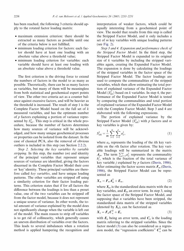
A geochemical dataset was derived from 145sediment samples taken from Late Quaternarydeposits (Holocene and Pleistocene), mainly ofmeandering rivers, in the Rhine-Meuse delta,The Netherlands (see Fig. 1). Geochemical charac-terization of these deposits has been more exten-sively treated in van Helvoort (2003). As a resultof abundant channel avulsing during the Holocene(Stouthamer and Berendsen, 2000), a dense,stacked network of palaeo-channels exists causinga high degree of heterogeneity over short distances(see cross-section in Fig. 1). The sedimentary het-erogeneity translates into geochemical heterogene-ity because there are close relations between grainsize and mineralogy (Huisman and Kiden, 1998;Johnsson, 1993; Moura and Kroonenberg, 1990;Nesbitt and Young, 1996; Passmore and Macklin,1994; Tebbens et al., 2001). For this reason, thedeposits have been grouped into 6 sedimentary fa-cies (Table 1) based on textural and structuralproperties, using an existing facies classificationfor fluvial deposits (Miall, 1985, 1996) that hasbeen adapted to this region (Berendsen, 1984;Tornqvist et al., 1994). Each facies has been sam-pled at various locations and depths along severaltransects (Fig. 1), covering most of the composi-tional variation present in these deposits. The sed-iment samples were dried at 70 �C andmechanically ground (Herzog HSM apparatus).X-ray Fluorescence (XRF) was used for majorelement (Al2O3, CaO, Fe2O3, K2O, MgO, MnO,Na2O, P2O5, SiO2 and Ti2O), and trace element(As, Ba, Bi, Cd, Ce, Cr, Cs, Cu, Ga, La, Mo,Nb, Ni, Pb, Rb, S, Sb, Sn, Sr, Th, U, V, Y, Znand Zr) determinations. Loss on ignition (LOI)

was determined at 1150 �C. In addition, theCEC was determined on freeze dried sub samples(unground) using a standard buffered salt method(Hesse, 1971). For a selection of samples, theCEC determination was carried out in quadrupli-cates and in each batch of 32 samples 3 blanksand 3 ISE standards were analyzed. Soil OrganicMatter (SOM) and carbonate contents were deter-mined on ground samples by Thermal GravimetricAnalysis, using a LECO TGA 608 apparatus.Grain size analysis was done by laser-diffraction,after removal of the >2000 lm fraction by sieving,and removal of both organic matter and carbon-ates using standard methods (van Doesburg,1996). All samples were analyzed in duplicateusing a Coulter LS230 apparatus, which has adetection range between 0.04 and 2000 lm discret-ized into 116 grain size classes. Quality of all ana-lytical procedures was checked by incorporatingrandom duplicates and international standards.

Prior to statistical analysis, the data were checkedfor accuracy and measurement artefacts. The obser-vations for Bi, Cd,Ce, La,Mo, Sb, Sn, Th andUwereleft out of further analysis because over 10% of theobservations were below the detection limit. For theother elements, observations under detectionwere re-placed by 2/3 times the detection limit. In addition,log transformation was applied, which for most vari-ables yielded improved normal distributions, or atleast improved symmetry. In the non-robust or classi-cal PCA, the removal of obvious outliers was com-bined with the first step of the seqFA procedure (seeSection 2.2).

The authors realize that compositional data isalways subject to (some degree of) data closure,because major components analysis usually sumup to 100% (Aitchison, 1981, 1984; Otero et al.,2005). Aitchison (1981) introduced the log-ratiotransformation, which diminishes data closure byeliminating the constant-sum and associated cur-vature in the data set. However, a log-ratio trans-formation was not applied, because the authorspreferred as few data manipulations as possiblewhile focussing on the new approach to factoranalysis. Instead of log-ratio transformation, themajor component analysis was not normalizedon 100%, leading to ‘‘open’’ total analyses varyingbetween 97% and 104%. Also, it was found thatcurvature in the data was scarce but present,and was reduced after log transformation of allcomponents. In addition, SiO2 was excluded fromfactor analysis, being the dominant component in

Fig. 1. Location of case study field area, sampling sites, and geological transect.


most samples (up to 95 wt%). The a priori re-moval of SiO2 therefore reduced the presence ofcurvatured relation ships down to a minimum,

while the most relevant geochemical relations werepreserved. This approach seemed to be satisfyingfor the goals of this paper.

Table 1Facies units, facies properties, and sample classification

Facies unit Lithology Geometry Number of samples

Channel deposits Very fine to coarse sand (105–2000 lm) 5–10 m thick, 50–2000 m wide 43Natural levee andcrevasse-splay deposits

Horizontally laminated sandy–silty clay,small lenses of (very) fine sand (105–210 lm)

Levees: 0.5–1.10 m thick,50–500 m wide; crevasse-splays:1–2 m thick, 0.1–5 km wide

23

Flood basin deposits Massive to very thin laminated clay and humic clay 1–5 m thick, 0.1–10�s km wide 30Organic deposits Peat 0.1–5 thick, 0.1–10�s km wide 20Eolian dune deposits Structureless of very fine to fine sand (105–210 lm) 1–10 m thick, 50–2000 m wide 17Loam bed deposits Massive sandy–clay to clayey sand; clay in

admixture with sand in the fraction 210–300 lm0.1–1.5 m thick, 1–10�s km wide 12

Total 145


2.2. Sequential Factor Analysis approach

2.2.1. General approach

The general procedure of the seqFA approach issummarized in Fig. 2, which shows the 4 consecutivesteps. Defining k, m and n as integers, and definingk = m + n, these steps can be explained as follows:

1. Define the optimum number of factors (andremove obvious outliers when using non-robustmethods). The resulting factor model is calledthe Complete Factor Model based on kmeasuredvariables.

2. Reduce the number of k variables to a set of mkey variables, by stripping off n highly correlatedvariables. The result is the Stripped FactorModel, with only m key variables.

Fig. 2. The general procedure of seqF

3. Expand the Stripped Factor Model with m keyvariables back to its full size of k variables by cal-culating the loadings for the stripped variables.The result is the Expanded Factor Model.

4. Compare the Expanded Factor Model with theComplete Factor Model in terms of explainedvariance.

Step 1. Optimizing the number of factors extracted

and identifying outliers. The optimum number offactors (step 1 in Fig. 2) is found by an iterative pro-cess, in which the number of factors (to which anyrotation method may be applied), is increased byone at a time, starting from a minimum of twofactors. Each time the factor model is extended bya new factor, the distributions of the loadings areexamined. When the optimum factor configuration

A, indicating the 4 main steps.


has been reached, the following 3 criteria should ap-ply to the rotated factor loading matrix:

• maximum extension criterion: there should beextracted as many factors as possible until oneof the criteria below is not fulfilled;

• minimum loading criterion for factors: each fac-tor should have at least one loading with anabsolute value above a threshold value;

• minimum loading criterion for variables: eachvariable should have at least one loading withan absolute value above a threshold value.

The first criterion is the driving force to extendthe numbers of factors in the model to as many aspossible. Theoretically, there can be as many factorsas variables, but many of them will be meaninglessfrom both statistical and geochemical expert pointsof view. The other two criteria act as a counter bal-ance against excessive factors, and will be heavier asthe threshold is increased. The result of step 1 is theComplete Factor Model based on the full set of kmeasured variables, and has the optimum numberof p factors explaining a portion of variance repre-sented by S2

kC. This step is critical in the whole pro-cedure, because the number of factors determineshow many sources of variance will be acknowl-edged, and how many unique geochemical processesor properties can be isolated from the dataset. In thecase of classical PCA, also the removal of obviousoutliers is included in this step (see Section 2.2.2).

Step 2. Selecting the key variables by variable

stripping. In this step, the number (m) and identityof the principal variables that represent uniquesources of variance are identified, giving the factorsdiscerned in the Complete Factor Model their coreor �key� identity. These principal variables are there-fore called key variables, and have unique loadingpatterns. The other variables are stripped off usinga similarity criterion for their factor loading pat-terns. This criterion states that if for all factors thedifference between the loadings is less than a presetvalue, one of the two variables can be stripped offfrom the factor model, because it does not representa unique source of variance. In other words, the to-tal amount of variance explained by the model doesnot significantly change when the variable is left outof the model. The main reason to strip off variablesis to get rid of collinearity, which generally causesan uneven distribution of variables over the factors.This leads to several imbalances when a rotationmethod is applied hampering the recognition and

interpretation of weaker factors, which could beequally interesting from a geochemical point ofview. The model that results from this step is calledthe Stripped Factor Model, and it only includes aset of m key variables with unique loading patterns(see Fig. 2).

Step 3 and 4. Expansion and performance check of

the Stripped Factor Model. In the third step, theStripped Factor Model is expanded to its originalsize of k variables by including the stripped vari-ables again, creating the Expanded Factor Model.The expansion is done by calculating the loadingsof the stripped variables in the factor space of theStripped Factor Model. The factor loadings areused to compute the communalities of the strippedvariables, which then allow estimating the total por-tion of explained variance of the Expanded FactorModel ðS2

kEÞ based on k variables. In step 4, the per-formance of the Expanded Factor Model is testedby comparing the communalities and total portionof explained variance of the Expanded FactorModelwith the Complete Factor Model. Step 3 and 4 areelaborated with the following expressions.

The portion of explained variance by theStripped Factor Model ðS2

mSÞ with p factors and m

key variables is given by:

S2mS ¼

1

m

Xmi¼1

Xp

r¼1

a2ir; ð1Þ

where air represents the loading of the ith key vari-able on the rth factor after rotation. The key vari-able loadings will be summarized in the matrixAm. The term

Ppr¼1a

2ir represents the communality

h2i , which is the fraction of the total variance ofkey variable j explained by p factors (Davis, 1986).After estimating the factor scores matrix Fm (Davis,1986), the Stripped Factor Model can be repre-sented as

Xm ¼ FmATm þ Em; ð2Þ

where Xm is the standardized data matrix with the mkey variables, and Em an error term. In step 3, usingthe factor space of the Stripped Factor Model, andsupposing that n variables have been stripped, thestandardized data matrix of the stripped variables(denoted by Xn), can be factorized as

Xn ¼ FmCTn þ En ð3Þ

with En being an error term, and Cn is the loadingmatrix referring to the stripped variables. Since thefactor model (3) can also be considered as a regres-sion model, the ‘‘regression coefficients’’ CT

n can be


estimated by multivariate linear regression (Johnsonand Wichern, 1998). For a more formal representa-tion on the estimation of the loadings Cn is given inFilzmoser (1997). Now, the portion of explainedvariance of n stripped variables in the ExpandedFactor Model is analogous to (1):

S2nE ¼ 1

n

Xn

j¼1

Xp

r¼1

c2jr ð4Þ

with cjr being an element of Cn, representing the esti-mated loading of the jth stripped variable on the rthfactor. Also,

Ppr¼1c

2jr represents the communality h2j

of the stripped variable j. Combining expressions (1)and (4), the portion of explained variance by theExpanded Factor Model ðS2

kEÞ with k variables canbe calculated:

S2kE ¼ m

mþ n

� �S2mS þ

nmþ n

� �S2nE. ð5Þ

In the evaluation step 4, the overall performance ofthe Stripped Factor Model can be expressed as theratio of the explained portions of variance by theExpanded Factor Model ðS2

kEÞ and the CompleteFactor Model ðS2

kCÞ:

Model performance ¼ S2kE

S2kC

. ð6Þ

Accordingly, the performance per variable can beexpressed as the ratio of communalities in the Ex-panded Factor Model and the Complete FactorModel for any variable k:

Variable performance ¼ h2kEh2kC

. ð7Þ

With these two indicators, the effect of stripping offvariables on both the overall portion of explainedvariance and the individual communalities can beassessed.

2.2.2. Computational procedures and outlier

replacement

All statistical computations were made in the Renvironment (version, 1.9.1), a powerful statisticalsoftware package which is freely available athttp://www.R-project.org. PCA was performed onthe correlation matrix with Varimax rotation (Kai-ser, 1958). Although any FA method can be used in-stead in combination with the seqFA procedure, wepreferred PCA here because it is the simplest multi-variate method and needs no additional assump-

tions. Hence, the authors used a slightly adaptedversion of an R-function initially designed for Prin-cipal Factor Analysis (PFA), but setting the unique-nesses all to zero. For the robust version, the fastMCD algorithm (Pison et al., 2003; Rousseeuwand van Driessen, 1999) was used to calculate therobust correlation matrix, based on 75% of the data.Thus, a maximum amount of 25% of outliers mightbe present in the data without affecting the estima-tion of the correlation matrix, which is consideredacceptable (see Pison et al. (2003)).

For the non-robust PCA, the classical samplecorrelation matrix was used, after some obviousoutliers were replaced by median values. First, po-tential outliers were identified by box plots and Q–Q plots. Second, as a part of the step 1 of seqFA,the factor score distributions of the unrotatedPCA model were examined on extreme values, pro-duced by outliers. The outliers responsible for ex-treme factor scores were eliminated one by onethrough substitution of median values of the faciesto which the cases belonged. It was decided not toleave out the entire case, because the observationsfor the other variables were not marked as outliersand should not disturb the PCA model. This was re-peated, until the unrotated PCA model produced noextreme factor scores anymore. This resulted inreplacement of only 6 observations (for Fe2O3,MnO, and P2O5), occurring in 3 cases, and 2 ofthem belonging to the organic deposits. The extremevalues were associated with dense concentrations ofvivianite or Fe/Mn-(hydr)oxides, which had alreadybeen spotted during field sampling. Note that thenumber of replacements was very small comparedto the whole data array of 3915 observations (145cases times 27 variables). The rest of the computa-tional procedure is explained below.

Step 1. In step 1 of seqFA, PCA was repeatedwhile increasing the number of factors one by one,until the loading matrix did not meet with one ofthe minimum loading criteria. The largest factorconfiguration that still fulfilled all criteria wasmarked as the optimum configuration, being themaximum number of factors that should be in-cluded in the Complete Factor Model. The mini-mum loading criteria were set to 0.60 for robustand non-robust PCA, this will be discussed furtherin the Section 3.1.1.

Step 2. In step 2, variable stripping was appliedto the loading matrix belonging to the optimumconfiguration selected in the previous step. Variablestripping was done as follows:

http://www.R-project.org

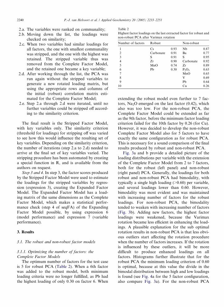
Table 2Highest factor loadings on the last extracted factor for robust andnon-robust PCA after Varimax rotation

Number of factors Robust Non-robust

1 Cs 0.93 Nb 0.872 Carbonate 0.91 Ba 0.773 S 0.91 S 0.954 Zr 0.90 Carbonate 0.925 MnO 0.74 Zr 0.896 Pb 0.30 P2O5 0.637 MnO 0.658 V 0.699 Pb 0.64

10 Cu 0.26


2.a. The variables were ranked on communality;2.b. Moving down the list, the loadings were

checked on similarity;2.c. When two variables had similar loadings for

all factors, the one with smallest communalitywas stripped, and the one with the highest wasretained. The stripped variable thus wasremoved from the Complete Factor Model,and the retained one became a key variable;

2.d. After working through the list, the PCA wasrun again without the stripped variables togenerate a new rotated loading matrix, butusing the appropriate rows and columns ofthe initial (robust) correlation matrix esti-mated for the Complete Factor Model;

2.e. Step 2.a through 2.d were iterated, until nofurther variables could be stripped off accord-ing to the similarity criterion.

The final result is the Stripped Factor Model,with key variables only. The similarity criterion(threshold for loadings) for stripping off was variedto see how this would influence the resulting set ofkey variables. Depending on the similarity criterion,the number of iterations (step 2.a to 2.d) needed toarrive at the final set of key variables varied. Thestripping procedure has been automated by creatinga special function in R, and is available from theauthors on request.

Step 3 and 4. In step 3, the factor scores producedby the Stripped Factor Model were used to estimatethe loadings for the stripped variables by regres-sion (expression 3), creating the Expanded FactorModel. The Expanded Factor Model has a load-ing matrix of the same dimensions as the CompleteFactor Model, which makes a statistical perfor-mance check (step 4 of seqFA) of the ExpandingFactor Model possible, by using expression 6(model performance) and expression 7 (variableperformance).

3. Results

3.1. The robust and non-robust factor models

3.1.1. Optimizing the number of factors: the

Complete Factor Models

The optimum number of factors for the test caseis 5 for robust PCA (Table 2). When a 6th factorwas added to the robust model, both minimumloading criteria were no longer fulfilled, as Pb hadthe highest loading of only 0.30 on factor 6. When

extending the robust model even further to 7 fac-tors, Na2O emerged on the last factor (0.42), whichalso was too low. For the non-robust PCA, theComplete Factor Model could be extended as faras the 9th factor, before the minimum factor loadingcriterion failed for the 10th factor by 0.26 (for Cu).However, it was decided to develop the non-robustComplete Factor Model also for 5 factors to haveexactly the same configuration as for robust PCA.This is necessary for a sound comparison of the finalresults produced by robust and non-robust PCA.

Fig. 3a and b provide a detailed picture of theloading distributions per variable with the extensionof the Complete Factor Model from 2 to 7 factors,both for the robust (left panel) and non-robust(right panel) PCA. Generally, the loadings for bothrobust and non-robust PCA had bimodality, withtypically a single high loading (>0.60) per variable,and several loadings lower than 0.60. However,bimodality was most evident and was maintainedwith increasing number of factors for the robustloadings. For non-robust PCA, the bimodalitytended to weaken with increasing number of factors(Fig. 3b). Adding new factors, the highest factorloadings were weakened, because the Varimaxrotation became less efficient in enhancing the load-ings. A plausible explanation for the sub optimalrotation results in non-robust PCA is that less obvi-ous outliers start affecting the rotation procedurewhen the number of factors increases. If the rotationis influenced by these outliers, it will be moredifficult to produce enhanced loadings on allfactors. Histograms further illustrate that for therobust PCA the minimum loading criterion of 0.60is optimal, because at this value the divide in thebimodal distribution between high and low loadingsis found (see Fig. 4a for the 5 factor configuration,also compare Fig. 3a). For the non-robust PCA

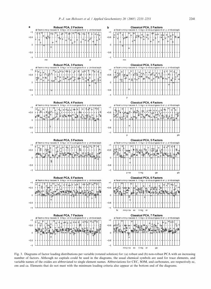
Fig. 3. Diagrams of factor loading distributions per variable (rotated solution) for: (a) robust and (b) non-robust PCA with an increasingnumber of factors. Although no capitals could be used in the diagrams, the usual chemical symbols are used for trace elements, andvariable names of the oxides are abbreviated to single element names. Abbreviations for CEC, SOM, and carbonates, are respectively ec,om and ca. Elements that do not meet with the minimum loading criteria also appear at the bottom end of the diagrams.


1.0.9.8.7.6.4.3.2.1.0

Absolute factor loading

1.0.9.8.7.6.4.3.2.1.0

Absolute factor loading

Fre

quen

cyF

requ

ency

20

15

10

5

0

40

30

20

10

0

a

b

Fig. 4. Bimodality of absolute factor loadings for the: (a) robustand (b) non-robust PCA configuration of 5 factors (rotatedsolution).


an optimal threshold for minimum loadings cannotactually be defined (Figs. 4b and 3b), hence also theoptimum number of factors could not objectively bederived (Table 2). This further justifies the choice ofa 5 factor model also for the non-robust case.

Anotherway to visualize the progressive extensionof theComplete FactorModels is presented inFig. 5aandb.These diagrams showper factorwhich variablehad the highest loading (i.e., the principal variable),depict the relations between consecutive factor con-figurations, and give a brief geochemical interpreta-tion. The extension of the robust Complete FactorModel shows a very regular pattern, as all new factorsoriginated from the first or the second factor. This isindicated by the dotted connections between the prin-cipal variables of the new factors and the factors onwhich they previously had the highest loadings. In

addition, there were very few changes in principalvariable of the same factor, and all factors remainedin the same order with respect to the relative portionof variance explained. The diagram for non-robustPCA is very different, with several changes of princi-pal variables, and factors that swapped position. Thisirregular pattern is evidence for instability of themodel, as the factors changed identity and rank whenincluding more factors for Varimax rotation. Thus,increasing the number of factors, the whole modelchanged fundamentally, because the Varimax rota-tion was very susceptible to a newly included sourceof variance. From these diagrams it is concluded thatrobust PCA yields much more stable – i.e., less sensi-tive to the number of factors chosen – and betterreproducible results than non-robust PCA.

3.1.2. Selection of key variables: The Stripped Factor

Models

Table 3 lists the key variable sets for the 5 factorconfiguration resulting from different similarity cri-teria for the robust and non-robust Stripped FactorModels. As expected, the number of stripped vari-ables always increased with decreasing strictness ofthe similarity criterion (from 0.10 to 0.30). Whensimilarity was set to 0.40 or more, the 5 factor con-figuration was not supported by the remaining set ofkey variables in terms of the minimum loading cri-teria defined previously, and therefore was consid-ered invalid.

The composition of the key variable set was quitesimilar for the robust and non-robust PCA,although the stripping usually proceeded more effi-ciently for the robust PCA (mostly one iteration)versus the non-robust PCA (2 or 3 iterations). Witha similarity of 0.30, the common key variables iden-tified are Cs, MnO, S, Na2O, Zr, Sr, SOM, andAl2O3, in order of decreasing communality ratios(see expression 7). The non-robust solution has onemore variable (Y) in the Stripped Factor Model.Thus, it is concluded that for the selected factor con-figuration with 5 factors, the robust and non-robustPCA Stripped Factor Models are highly congruent.The results for the most condensed Stripped FactorModels, i.e., with a similarity stated at 0.30, will bediscussed quantitatively in the next section.

3.1.3. The Expanded Factor Models and statistical

performance

Tables 4A and 4B show the factor loadings(>0.30) for the Complete Factor Model and theExpanded Factor Model, both for the robust

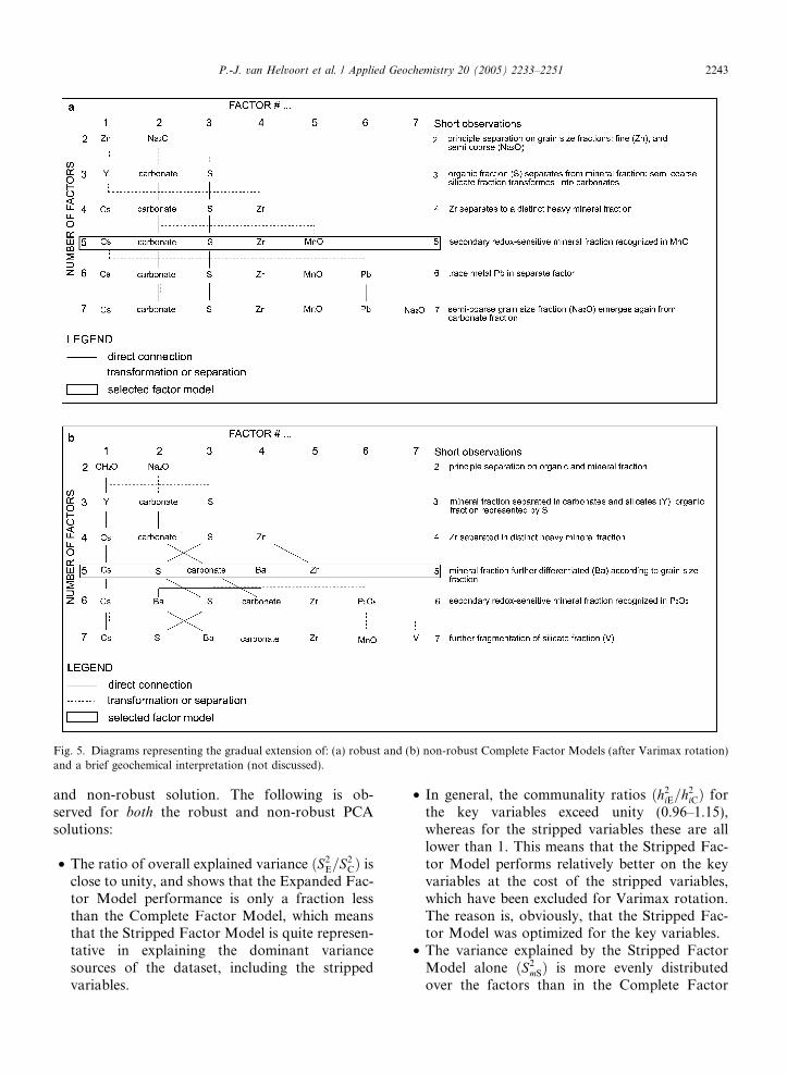
Fig. 5. Diagrams representing the gradual extension of: (a) robust and (b) non-robust Complete Factor Models (after Varimax rotation)and a brief geochemical interpretation (not discussed).


and non-robust solution. The following is ob-served for both the robust and non-robust PCAsolutions:

• The ratio of overall explained variance ðS2E=S

2CÞ is

close to unity, and shows that the Expanded Fac-tor Model performance is only a fraction lessthan the Complete Factor Model, which meansthat the Stripped Factor Model is quite represen-tative in explaining the dominant variancesources of the dataset, including the strippedvariables.

• In general, the communality ratios ðh2iE=h2iCÞ forthe key variables exceed unity (0.96–1.15),whereas for the stripped variables these are alllower than 1. This means that the Stripped Fac-tor Model performs relatively better on the keyvariables at the cost of the stripped variables,which have been excluded for Varimax rotation.The reason is, obviously, that the Stripped Fac-tor Model was optimized for the key variables.

• The variance explained by the Stripped FactorModel alone ðS2

mSÞ is more evenly distributedover the factors than in the Complete Factor

Table 3Key variable sets (>0.30) for the 5-factor configuration with different similarity criteria for variable stripping, both for robust and non-robust Stripped Factor Models

All variables Robust Stripped Factor Models Non-robust Stripped Factor Models

0.10 0.15 0.20 0.25 0.30 0.10 0.15 0.20 0.25 0.30

Al2O3 Al2O3 Al2O3 Al2O3 Al2O3 Al2O3 Al2O3 Al2O3 Al2O3 Al2O3 Al2O3

As As As As AsBa Ba Ba BaCarbonate Carbonate Carbonate CarbonateCECCr CrCs Cs Cs Cs Cs Cs Cs Cs Cs Cs CsCu Cu Cu Cu Cu CuFe2O3 Fe2O3 Fe2O3

GaK2O K2O K2O K2O K2OMgOMnO MnO MnO MnO MnO MnO MnO MnO MnO MnO MnONa2O Na2O Na2O Na2O Na2O Na2O Na2O Na2O Na2O Na2O Na2ONb Nb Nb NbNiPb Pb PbP2O5 P2O5 P2O5 P2O5 P2O5 P2O5 P2O5 P2O5

Rb RbS S S S S S S S S S SSOM SOM SOM SOM SOM SOM SOM SOM SOM SOMSr Sr Sr Sr Sr Sr Sr Sr Sr Sr SrTiO2 TiO2 TiO2 TiO2 TiO2 TiO2 TiO2

V V V VY Y Y Y Y Y Y YZn Zn Zn Zn Zn ZnZr Zr Zr Zr Zr Zr Zr Zr Zr Zr Zr


Model (compare S2mS with S2

C for the individualfactors in Tables 4A and 4B). The reason is thatin the Complete Factor Model most high load-ings were found on the first factor (F1), andtherefore this factor explains the larger part ofthe variance. However, in the Stripped FactorModel the highest loadings are more evenly dis-tributed over the factors, because much of thecollinearity has been removed by variablestripping.

Comparing results between the robust and non-robust solution, it is evident that the results forthe Stripped/Extended Factor Model are far moresimilar to each other than those for the CompleteFactor Model. For the Complete Factor Models,the Varimax rotation obviously leads to distinctlydifferent orientations of the principal axes. The dif-ference is also evident in the communalities of the(key) variables. The Stripped/Expanded Modelsshow highly similar orientations, but for a shufflingof ranks between F3 and F4, and also very similarcommunalities.

The main implications of these results are 4-fold.First of all, the Stripped Factor Model is the mostcondensed way to summarize the main sources ofvariance in a geochemical dataset, without loosingany key information, and without loosing signifi-cant explained variance via the Expanded FactorModel. Secondly, the Stripped Factor Model yieldshigher loadings for the remaining key variables,which facilitates interpretation of the factors.Thirdly, the Stripped Factor Model enhances weak-er factors at the cost of stronger ones. This validatesthe extraction of weaker factors with smaller eigen-values in the first step of the seqFA. Finally, theStripped (and Extended) Factor Model is morerobust to outliers in minor variables than the Com-plete Factor Model.

3.2. A conceptual geochemical model for riverine

deposits

3.2.1. Interpretation of the factors

The loading matrix of the robust ExpandedFactor Model (Table 4A) was used to develop a

Table 4AFactor loadings (>0.30) for the robust Complete and Expanded Factor Model (variables sorted on communality ratiosb)

Complete Factor Model Expanded Factor Model E/Cb

F1 F2 F3 F4 F5 Communality F1 F2 F3 F4 F5 Communality

Csa 0.92 0.88 0.96 0.97 1.11MnOa 0.35 0.52 0.65 0.90 0.91 0.98 1.09Sa 0.31 0.90 0.91 0.94 0.98 1.07Na2O

a 0.76 0.44 0.94 0.89 0.33 0.97 1.02Zra 0.30 0.90 0.97 0.91 0.99 1.02Sra 0.35 0.86 0.94 0.73 0.53 0.95 1.01SOMa 0.70 0.59 0.97 0.60 0.63 0.39 0.97 1.00Al2O3

a 0.86 0.33 0.99 0.75 0.36 0.31 0.31 0.95 0.96

TiO2 0.75 0.31 0.31 0.47 0.99 0.62 0.36 0.34 0.50 0.96 0.98Y 0.83 0.38 0.97 0.74 0.31 0.32 0.44 0.95 0.98CEC 0.77 0.45 0.95 0.66 0.48 0.36 0.34 0.92 0.97Fe2O3 0.79 0.35 0.97 0.67 0.38 0.47 0.32 0.95 0.97Ni 0.78 0.32 0.30 0.92 0.67 0.38 0.38 0.34 0.90 0.97Cr 0.78 0.33 0.35 0.35 0.98 0.64 0.41 0.35 0.39 0.94 0.96MgO 0.81 0.35 0.32 0.97 0.69 0.39 0.39 0.93 0.96Nb 0.83 0.37 0.91 0.76 0.42 0.88 0.96Rb 0.86 0.37 0.98 0.74 0.38 0.32 0.35 0.94 0.96Zn 0.83 0.42 0.97 0.71 0.47 0.35 0.94 0.96V 0.83 0.38 0.98 0.71 0.43 0.36 0.31 0.94 0.96Carbonate 0.91 0.93 0.72 0.57 0.89 0.95Ga 0.85 0.30 0.34 0.97 0.72 0.41 0.33 0.92 0.95K2O 0.84 0.48 0.97 0.72 0.47 0.30 0.92 0.94Cu 0.83 0.36 0.87 0.72 0.43 0.32 0.81 0.93Pb 0.64 0.32 0.36 0.41 0.81 0.52 0.38 0.31 0.40 0.75 0.92As 0.58 0.69 0.89 0.47 0.64 0.35 0.81 0.91P2O5 0.63 0.43 0.46 0.86 0.51 0.58 0.78 0.91Ba 0.89 0.31 0.93 0.78 0.32 0.83 0.90

S2mS 0.26 0.20 0.19 0.18 0.14 0.97S2nE 0.43 0.15 0.08 0.14 0.09 0.89

S2kC 0.51 0.15 0.13 0.09 0.05 0.94 S2kE 0.38 0.16 0.11 0.15 0.11 0.92 0.97

a Key variables.b Ratio of communality in Expanded Factor Model (E) to Complete Factor Model (C).


geochemical model for the Late Quarternary depos-its in the Rhine-Meuse delta by interpreting eachfactor carefully. The factor scores were plotted inFig. 6 to illustrate the geochemical differences be-tween the facies. The non-robust Expanded FactorModel is not discussed in a separate section, becauseof its similarity to the robust model.

Factor 1. Variation in clay content. The first fac-tor represents the variation of the finest grain sizefraction in the riverine deposits. The factor scoresof F1 reflect the textural difference between faciesvery well, placing them in order of increasing claycontent. As a result of (hydrodynamic) sorting pro-cesses, clay content increases from eolian dune,channel, loam bed, crevasse-levee, organic to floodplain deposits (see Table 1). Note that in the organicdeposits the clastic matrix has been diluted by SOM,leading to lower clay contents than in the flood

plain deposits. Factor 1 has the highest loadingsfor the key variables Cs (0.96) and Al2O3 (0.75),and almost all other trace elements that have beenstripped off (Table 4A). Cesium is highly adsorptiveto clay mineral surfaces (Gier and Johns, 2000;Shahwan and Erten, 2001), whereas Al2O3 is themost important building block of clay minerals.However, contrary to other regional studies usingfactor analysis to describe geochemical variation insedimentary deposits (Huisman and Kiden, 1998;Moura and Kroonenberg, 1990; Tebbens et al.,2001), Al2O3 was not found to be the principal var-iable describing clay mineral content. The explana-tion is that Al2O3 does not occur uniquely in clayminerals, but also in other silicates that occur in lar-ger grain size categories (see F3).

Factor 2. Variation in reduced sulfur and SOM

contents. Factor 2 is interpreted as the variation in

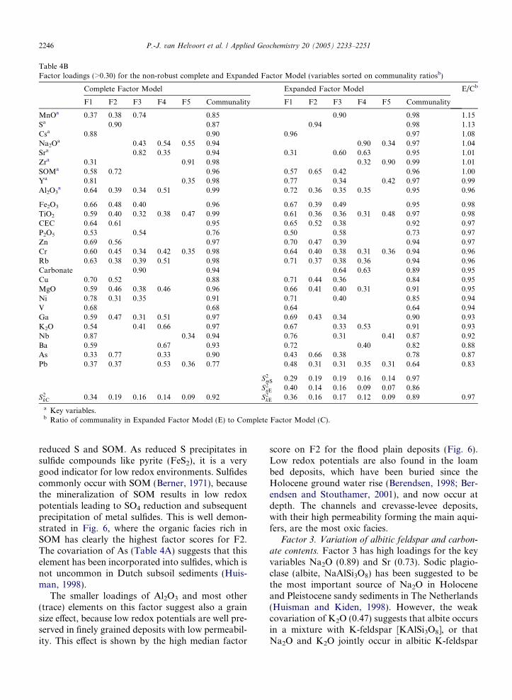
Table 4BFactor loadings (>0.30) for the non-robust complete and Expanded Factor Model (variables sorted on communality ratiosb)

Complete Factor Model Expanded Factor Model E/Cb

F1 F2 F3 F4 F5 Communality F1 F2 F3 F4 F5 Communality

MnOa 0.37 0.38 0.74 0.85 0.90 0.98 1.15Sa 0.90 0.87 0.94 0.98 1.13Csa 0.88 0.90 0.96 0.97 1.08Na2O

a 0.43 0.54 0.55 0.94 0.90 0.34 0.97 1.04Sra 0.82 0.35 0.94 0.31 0.60 0.63 0.95 1.01Zra 0.31 0.91 0.98 0.32 0.90 0.99 1.01SOMa 0.58 0.72 0.96 0.57 0.65 0.42 0.96 1.00Ya 0.81 0.35 0.98 0.77 0.34 0.42 0.97 0.99Al2O3

a 0.64 0.39 0.34 0.51 0.99 0.72 0.36 0.35 0.35 0.95 0.96

Fe2O3 0.66 0.48 0.40 0.96 0.67 0.39 0.49 0.95 0.98TiO2 0.59 0.40 0.32 0.38 0.47 0.99 0.61 0.36 0.36 0.31 0.48 0.97 0.98CEC 0.64 0.61 0.95 0.65 0.52 0.38 0.92 0.97P2O5 0.53 0.54 0.76 0.50 0.58 0.73 0.97Zn 0.69 0.56 0.97 0.70 0.47 0.39 0.94 0.97Cr 0.60 0.45 0.34 0.42 0.35 0.98 0.64 0.40 0.38 0.31 0.36 0.94 0.96Rb 0.63 0.38 0.39 0.51 0.98 0.71 0.37 0.38 0.36 0.94 0.96Carbonate 0.90 0.94 0.64 0.63 0.89 0.95Cu 0.70 0.52 0.88 0.71 0.44 0.36 0.84 0.95MgO 0.59 0.46 0.38 0.46 0.96 0.66 0.41 0.40 0.31 0.91 0.95Ni 0.78 0.31 0.35 0.91 0.71 0.40 0.85 0.94V 0.68 0.68 0.64 0.64 0.94Ga 0.59 0.47 0.31 0.51 0.97 0.69 0.43 0.34 0.90 0.93K2O 0.54 0.41 0.66 0.97 0.67 0.33 0.53 0.91 0.93Nb 0.87 0.34 0.94 0.76 0.31 0.41 0.87 0.92Ba 0.59 0.67 0.93 0.72 0.40 0.82 0.88As 0.33 0.77 0.33 0.90 0.43 0.66 0.38 0.78 0.87Pb 0.37 0.37 0.53 0.36 0.77 0.48 0.31 0.31 0.35 0.31 0.64 0.83

S2mS 0.29 0.19 0.19 0.16 0.14 0.97S2nE 0.40 0.14 0.16 0.09 0.07 0.86

S2kC 0.34 0.19 0.16 0.14 0.09 0.92 S2kE 0.36 0.16 0.17 0.12 0.09 0.89 0.97

a Key variables.b Ratio of communality in Expanded Factor Model (E) to Complete Factor Model (C).


reduced S and SOM. As reduced S precipitates insulfide compounds like pyrite (FeS2), it is a verygood indicator for low redox environments. Sulfidescommonly occur with SOM (Berner, 1971), becausethe mineralization of SOM results in low redoxpotentials leading to SO4 reduction and subsequentprecipitation of metal sulfides. This is well demon-strated in Fig. 6, where the organic facies rich inSOM has clearly the highest factor scores for F2.The covariation of As (Table 4A) suggests that thiselement has been incorporated into sulfides, which isnot uncommon in Dutch subsoil sediments (Huis-man, 1998).

The smaller loadings of Al2O3 and most other(trace) elements on this factor suggest also a grainsize effect, because low redox potentials are well pre-served in finely grained deposits with low permeabil-ity. This effect is shown by the high median factor

score on F2 for the flood plain deposits (Fig. 6).Low redox potentials are also found in the loambed deposits, which have been buried since theHolocene ground water rise (Berendsen, 1998; Ber-endsen and Stouthamer, 2001), and now occur atdepth. The channels and crevasse-levee deposits,with their high permeability forming the main aqui-fers, are the most oxic facies.

Factor 3. Variation of albitic feldspar and carbon-

ate contents. Factor 3 has high loadings for the keyvariables Na2O (0.89) and Sr (0.73). Sodic plagio-clase (albite, NaAlSi3O8) has been suggested to bethe most important source of Na2O in Holoceneand Pleistocene sandy sediments in The Netherlands(Huisman and Kiden, 1998). However, the weakcovariation of K2O (0.47) suggests that albite occursin a mixture with K-feldspar [KAlSi3O8], or thatNa2O and K2O jointly occur in albitic K-feldspar

Fig. 6. Boxplots showing the factor score distributions per factor and per facies. Boxes represent interquartiles, with median indicated bythe horizontal bar. Whiskers show maximum and minimum scores that fall within 1.5 times the interquartile range of the box measuredfrom the upper and lower quartiles, respectively.

0 0.4 0.8 1.2Na2O (wt%)

0

0. 4

0. 8

1. 2

1. 6

2

K2O

(wt%

)

Fig. 7. K2O vs. Na2O (weight percentages) for the sandy eoliandune and channel facies.


[(Na,K)AlSi3O8]. Fig. 7 shows a steady increase ofK with Na in a ratio of about 3:2 (weight percent-ages) in the sandy facies, suggesting that the albiticK-feldspar or the mineralogical mixture has aconstant composition. According to Fig. 8, these sil-icates are enriched in the 20–150 lm grain size frac-tion, and should be abundant in the channel, eoliandune and crevasse-levee facies. The weak loadingfor Al2O3 on this factor confirms that the variation

of Al2O3 is not solely dictated by clay mineralcontent.

The high loading for Sr translates into the varia-tion of carbonate content, because Sr is a commonsubstitute for Ca in carbonates and aragonites(Kinsman and Holland, 1969). This is clear fromthe identical loading patterns for Sr and carbonatein the Expanded Factor Model. In these deposits,carbonate has mainly been identified as being pres-ent as detrital fragments of biogenic origin, whichhave been concentrated in silty facies (crevasse-leveedeposits) along with Na-bearing silicates (see Fig. 6)because of their similar weight. For this reason, car-bonate content covaries with Na2O content, andloads on the same factor.

As F3 has a mixed geochemical significance, thefactor score distributions in Fig. 6 should be inter-preted with care. On geochemical grounds, it mightbe better to consider the principal variables sepa-rately, i.e., the Na2O and Sr/carbonate contents.Though Table 4A and Fig. 8 suggest high carbonatecontents occurring with intermediate grain sizes, forthe eolian dune facies this relation is not present be-cause all carbonate was leached out during the EarlyHolocene when the eolian dunes were uncovered.The covariation of carbonate and feldspar contentsin the crevasse-levee facies tends to dominate this

-1

-0.5

0

0.5

1

Co

rre

latio

n

CLAY SILT VFS FS CS

Na2O

Cs

carbonates

Zr

0.10 µm 8.0 µm 50.0 µm 150 µm 2000 µm

Grain size classes (0.10 -2000 µm)

Fig. 8. Correlation of selected key variables to laser particle data (0.10–2000 lm).


relationship, but it should be assessed for the otherfacies individually.

Factor 4. Variation in Mn and P mineral contents.

This factor has the highest loading for key variableMnO (0.91), and weaker loadings for P2O5, Fe2O3,carbonate, and Sr. The factor is interpreted as thevariation in secondarily formed Mn and P-bearing minerals like Mn-(hydr)oxides, vivianite[Fe3(PO4)2 Æ 8H2O], and apatite [Ca5(PO4)3(OH)].In aquifer sediments, Mn (hydr)oxides commonlyoccur with Fe(III)-(hydr)oxides under (sub)oxicconditions (Appelo and Postma, 1994; Heron andChristensen, 1994; Larsen and Postma, 1997), whilevivianite has been reported as a sink for P andFe(II) in anaerobic, clayey abandoned channeldeposits of the Meuse river (Tebbens et al., 1999).In addition, apatite forms under alkaline conditionsin the presence of Ca, which is often the case in theshallow subsoil under arable land as a result ofexcessive Ca and P-fertilizer application (Sposito,1989). Hence, MnO, P2O5 and Fe2O3 are relatedvia secondary mineral phases and therefore occurin the same factor. Fig. 6 shows that the organicand crevasse-levee deposits have been enriched inMn/P bearing minerals. This is complementary tofield observations of vivianite occurrence in reducedorganic deposits, and Mn/Fe (hydr)oxides in sub-oxic crevasse-levee deposits occurring close to theground water table. The covariation of Sr/carbonatewith MnO largely follows grain size (see Fig. 8), be-cause the silty crevasse-levee facies is enriched in bothFe/Mn (hydr)oxides and carbonates. The eoliandune deposits are depleted of Mn/P minerals.

Factor 5. Variation in heavy mineral content. Thisfactor has the highest loading for Zr, and weakerones for TiO2, Nb, and Y. It is interpreted as reflect-ing the variation in heavy mineral content, includingzircon (Zr), rutile (TiO2), and associated trace ele-

ments Nb and Y, which are known to be least mo-bile during weathering processes (Humphris andThompson, 1982; Thompson, 1973). Fig. 8 suggestthat Zr is enriched in the silt fraction, and Fig. 6confirms that heavy minerals have indeed beenenriched in the silty crevasse-levee and loam bed fa-cies. In addition, heavy minerals have been enrichedin the sandy eolian dune facies, which are not silty.The explanation is that the sandy eolian dunes havebeen depleted of most other components by leach-ing and eolian sorting processes, leaving a relativeconcentration of heavy minerals.

3.2.2. A conceptual geochemical model

The robust Expanded Factor Model can betranslated into a conceptual geochemical model,describing the chemical variation in the sedimen-tary deposits of the Rhine-Meuse delta plain interms of independent physical and chemical pro-cesses. This approach is very similar to Mengand Maynard (2001), who formulated a conceptualmodel describing the dominant processes governingwater chemistry in a Brazilian aquifer. Tables 5Aand 5B list the 4 processes derived from the Ex-panded Factor Model, being: depositional sorting,peat formation, redox processes, and dissolution/precipitation of secondary minerals. These pro-cesses have been grouped as either syn-depositionalor post-depositional processes.

Table 5A shows that F1 and F5 represent onlyone process, whereas the other factors incorporateseveral processes. For this reason, F1 and F5 arelabelled as ‘‘pure’’ factors, and F2, F3, and F4 as‘‘mixed’’ factors. The pure factors were easiest tointerpret but for the mixed factors, additionalgeochemical expertize or field observations areneeded to assess their meaning properly. Likewise,variables can be classified as ‘‘pure’’ or ‘‘mixed’’,

Table 5BRepresentation of governing processes by the key variables in the robust Expanded Factor Model

Process Cs Al2O3 SOM S Na2O Sr MnO Zr

Syn-depositionalDepositional sorting · · · · · · ·Peat formation · ·

Post-depositionalRedox · ·Precipitation/dissolution · ·

Table 5ARepresentation of governing processes by the individual factors of the robust Expanded Factor Model

Process F1 F2 F3 F4 F5

Syn-depositionalDepositional sorting (clay minerals, feldspar, heavy minerals, carbonate fragments) · · · ·Peat formation (SOM accumulation) ·

Post-depositionalRedox (formation of sulphides, Mn/Fe oxides, vivianite) · ·Precipitation/dissolution (carbonate leaching, apatite precipitation) · ·


dependent on whether they are associated with asingle or several processes. Table 5B shows thatthe key variables Cs, Al2O3, Na2O, and Zr are‘‘pure’’, and associated with only one process (syn-depositional grain sorting). The distribution ofother constituents has been affected by several pro-cesses, and thus are of the ‘‘mixed’’ type. Note thatTables 5A and 5B are complementary because a fac-tor can only be ‘‘pure’’ when the key variable withthe highest loading is ‘‘pure’’ as well.

It is concluded that the robust Expanded Modelis more than just 5 separated sources of varianceextracted from a geochemical dataset, but alsoaccurately describes many geochemical and miner-alogical properties of the sedimentary deposits inthe Rhine-Meuse delta. These properties can belinked to 4 governing independent physical andgeochemical processes, leading to a conceptualmodel that helps understanding of the geochemicalvariation of these deposits in detail.

4. Discussion and conclusions

Over the years, there has been extensive discussionabout how FA or PCA should be applied (Garrett,1993; Reimann and Filzmoser, 2000; Reimannet al., 2002). Important issues invariably have beenthe effect of outliers, and the number of factors andvariables that should be included in the multivariatesolution. The novel sequential approach presentedin this paper clarifies these issues substantially.

Using a heterogeneous geochemical dataset, theauthors took the opportunity to assess the effect ofmultivariate outliers on PCA by comparing the ro-bust and non-robust solutions. Using the robustestimate of the correlation matrix as input forPCA, it was observed from the gradual extensionof the Complete Factor Model that the rotated fac-tor solutions are very consistent whereas the non-robust solutions are not. Also, the change fromthe Complete Factor Model towards the Stripped/Extended Factor Model seems to be more moderatefor the robust solution. Therefore, it is concludedthat a robust approach is superior to a non-robustapproach, and the authors recommend alwaysapplying robust PCA or FA to geochemical data-sets, minimizing the effect of multivariate outlierson the rotated factor solutions.

The number of factors that should be extractedhas been identified in an objective manner. A mini-mum loading criterion has been identified from therotated loading distributions produced by robustPCA. The loading distributions showed a persistentbimodality, indicating that Varimax rotation worksoptimally for the robust case. The minimum loadingcriterion should therefore be set at the lower bound-ary of the high end distribution, and used for deter-mining objectively the optimum number of factorsthat should be extracted. This is an importantachievement of seqFA, because so far, there wereno adequate objective guides for factor extraction.However, the researcher may decide to deviate from


the optimum, but in doing so should realize that thefactor model tends to become over or underspecifiedwith too many or too few factors respectively.

The issue of variable extraction has been ad-dressed in a systematical approach. In this study,similarity criteria and communality sorting wereused to identify key variables. The results aretherefore objective and statistically optimized,highly condensed, and easy to interpret. However,the results could also be generated in a more flex-ible way. For instance, if researchers are interestedin trace element chemistry, they could manuallypreset for each factor the trace element with thehighest communality as the key variable.Although they would not find the statistical opti-mum, they would be developing the factor modeltowards trace element chemistry, because the fac-tor rotation is manipulated (optimized) towardsthe preset keys. This makes the variable strippingprocedure flexible, as the results can always bechecked by comparing the explained varianceand communalities of the Complete Factor Modeland the Expanded Factor Model.

In general, it is concluded that seqFA is a veryuseful approach to explore heterogeneous geochem-ical datasets multivariately. Using robust statistics,seqFA leads to a balanced set of factors and vari-ables, because the results are produced in severalsteps. Within each step, the researcher obtains newinformation concerning the multivariate structuresin the dataset, the stability of the factor model,and the developing identities of the extracted fac-tors. This opens the way to a broad range of appli-cations of robust PCA or FA, includingmultivariate outlier detection and stability analysis,variance source identification, and variable cluster-ing. In addition, the identification of hidden geo-chemical processes and properties is improvedrelative to traditional approaches. This appliedstudy demonstrates that with seqFA, the authorswere able to derive a consistent geochemical concep-tual model to explain the compositional variabilityof the heterogeneous Late Quaternary deposits inthe Rhine-Meuse delta (The Netherlands).

References

Aitchison, J., 1981. A new approach to null correlations ofproportions. Math. Geol. 13, 175–189.

Aitchison, J., 1984. Reducing the dimensionality of composi-tional data sets. Math. Geol. 16, 617–634.

Appelo, C.A.J., Postma, D., 1994. Geochemistry, Groundwaterand Pollution. Balkema, Rotterdam.

Basilevski, A., 1994. Statistical Factor Analysis and RelatedMethods. Theory and Applications. Wiley, New York.

Berendsen, H.J.A., 1984. Problems of lithostratigraphic classifi-cation of Holocene deposits in the perimarine area of theNetherlands. Geol. Mijnbouw 63, 351–354.

Berendsen, H.J.A., 1998. Birds-Eye view of the Rhine-Meusedelta (The Netherlands). J. Coastal Res. 14, 740–752.

Berendsen, H.J.A., Stouthamer, E., 2001. Late Weichselian andHolocene palaeogeography of the Rhine-Meuse delta, TheNetherlands. Palaeogeog. Palaeoclim. Palaeoecol. 161, 311–335.

Berner, R.A., 1971. Principles of Chemical Sedimentology.McGraw-Hill, New York.

Cameron, E.M., 1996. Hydrochemistry of the Fraser River,British Columbia: seasonal variation in major and minorcomponents. J. Hydrol. 182, 209–215.

Cattell, R.B., 1966. The scree test for the number of factors.Multivar. Behav. Res. 1, 245–276.

Chork, C.Y., Salminen, R., 1993. Interpreting explorationgeochemical data from Outokumpu, Finland: MVE-robustfactor analysis. J. Geochem. Explor. 48, 1–20.

Dalton, M., Upchurch, S., 1979. Interpretation of hydrochemicalfacies by factor analysis. Ground Water 16, 228–233.

Davis, J.C., 1986. Statistics and Data Analysis in Geology. Wiley,New York.

De Vivo, B., Boni, M., Marcello, A., Di Bonito, M., Russo, A.,1997. Baseline geochemical mapping of Sardinia (Italy). J.Geochem. Explor. 60, 77–90.

Duffy, C.J., Brandes, D., 2001. Dimension reduction and sourceidentification for multispecies groundwater contamination. J.Contam. Hydrol. 48, 151–165.

Evans, C.D., Davies, T.D., Wigington Jr., P.J., Tranter, M.,Kretser, W.A., 1996. Use of factor analysis to investigateprocesses controlling the chemical composition of fourstreams in the Adirondack Mountains, New York. J. Hydrol.185, 297–316.

Filzmoser, P., 1997. Finding structures of interest in a largedataset using factor analysis. Austrian J. Statistics 26, 27–34.

Frapporti, G., Vriend, S.P., van Gaans, P.F.M., 1993. Hydro-chemistry of the shallow Dutch groundwater; interpretationof the national ground water monitoring network. WaterResour. Res. 17, 2993–3004.

Garrett, R.G., 1993. Another cry from the heart. Explore 81, 9–14.

Gier, S., Johns, W.D., 2000. Heavy metal-adsorption on micasand clay minerals studied by X-ray photoelectron spectros-copy. Appl. Clay Sci. 16, 289–299.

Gupta, L.P., Subramanian, V., 1998. Geochemical factorscontrolling the chemical nature of water and sediments inthe Gomti River, India. Environ. Geol. 36, 102–108.

Hakstege, A.L., Kroonenberg, S.B., van Wijk, H., 1993. Geo-chemistry of Holocene clays of the Rhine and Meuse rivers inthe centra-eastern Netherlands. Geol. Mijnbouw 71, 301–315.

Heron, G., Christensen, T.H., 1994. The role of aquifer sedimentin controlling redox conditions in polluted groundwater. In:Dracos, T., Stauffer, F. (Eds.), Transport and ReactiveProcesses in Aquifers. Balkema, Rotterdam, pp. 73–77.

Hesse, P.R., 1971. Cation and anion exchange properties. In: ATextbook of Soil Chemical Analyses. John Murray, London,pp. 88–105.


Huisman, D.J., 1998. Geochemical Characterization of Subsur-face Sediments in The Netherlands. Netherlands Institute ofApplied Geoscience, TNO.

Huisman, D.J., Kiden, P., 1998. A geochemical record of LateCenozoic sedimentation history in the soutern Netherlands.Geol. Mijnbouw 76, 277–292.

Humphris, S.E., Thompson, G., 1982. A geochemical study ofrocks from the Walvis Ridge, South Atlantic. Chem. Geol. 36,253–274.

Johnson, R., Wichern, D., 1998. Applied Multivariate StatisticalAnalysis. Prentice-Hall, London.

Johnsson, M.J., 1993. The system controlling the composition ofclastic sediments. In: Johnsson, M.J., Basu, A. (Eds.),Geological Society of America Special Paper 284, vol. 284.GSA, pp. 1–19.

Kaiser, H.F., 1958. The Varimax criterion for analytic rotation infactor analysis. Psychometrika 23, 187–200.

Kinsman, D.J.J., Holland, H.D., 1969. The co-precipitation ofcations with CaCO3 – IV. The co-precipitation of Sr2+ witharagonite between 16 and 96 �C. Geochim. Cosmochim. Acta33, 1–17.

Larsen, F., Postma, D., 1997. Nickel mobilization in a ground-water well field: Release by pyrite oxidation and desorptionfrom manganese oxides. Environ. Sci. Technol. 31, 2589–2595.

Lawrence, F.W., Upchurch, S.B., 1982. Identification of rechargeareas using geochemical factor analysis. Ground Water 20,680–687.

Lee, J.Y., Cheon, J.Y., Lee, K.K., Lee, S.Y., Lee, M.H., 2001.Statistical evaluation of geochemical parameter distributionin a ground water system contaminated with petroleumhydrocarbons. J. Eviron. Qual. 30, 1548–1563.

Meng, S.X., Maynard, J.B., 2001. Use of statistical analysis toformulate conceptual models of geochemical behavior: waterchemical data from the Botucatu aquifer in Sao Paulo state,Brazil. J. Hydrol. 250, 78–97.

Miall, A.D., 1985. Architectural-elements analysis: a new methodof facies analysis applied to fluvial deposits. Earth-Sci. Rev.22, 261–308.

Miall, A.D., 1996. The Geology of Fluvial Deposits. Springer,Heidelberg.

Morsy, M.A., 1993. An example of application of factor analysison geochemical stream sediment survey in Umm Kharigaarea, Eastern Desert, Egypt. Math. Geol. 25, 833–850.

Moura, M.L., Kroonenberg, S.B., 1990. Geochemistry of Quar-ternary fluvial and eolian sediment in the southeasternNetherlands. Geol. Mijnbouw 69, 359–373.

Nesbitt, W., Young, G.M., 1996. Petrogenesis of sediments in theabsence of chemical weathering: effects of abrasion andsorting on bulk composition and mineralogy. Sedimentology43, 341–358.

Otero, N., Tolosana-Delgado, R., Soler, A., Pawlowsky-Glahn,V., Canals, A., 2005. Relative vs. absolute statisical analysisof compositions: A comparative study of surface waters of aMediterranean river. Water Res. 39, 1404–1414.

Passmore, D.G., Macklin, M.G., 1994. Provenance of fine-grained alluvium and late Holocene land-use change in theTyne basin, northern England. Geomorphology 9, 127–142.

Pison, G., Rousseeuw, P.J., Filzmoser, P., Croux, C., 2003.Robust factor analysis. J. Multivar. Anal. 84, 145–172.

Reimann, C., Filzmoser, P., 2000. Normal and lognormal datadistribution in geochemistry: dead of a myth. Consequencesof geochemical and environmental data. Environ. Geol. 39,1001–1014.

Reimann, C., Filzmoser, P., Garrett, R.G., 2002. Factor analysisapplied to regional geochemical data: problems and possibil-ities. Appl. Geochem. 17, 185–206.

Rousseeuw, P.J., van Driessen, A., 1999. A fast algorithm for theminimum covariance determinant estimator. Technometrics41, 212–223.

Shahwan, T., Erten, H.N., 2001. Thermodynamic parameters ofCs+ sorption on natural clays. J. Radioanal. Nucl. Chem.253, 115–120.

Sposito, G., 1989. The Chemistry of Soils. Oxford UniversityPress, New York/Oxford.

Stouthamer, E., Berendsen, H.J.A., 2000. Factors controlling theHolocene avulsion history of the Rhine-Meuse delta (TheNetherlands). J. Sed. Res. 70, 1051–1064.

Suk, H., Lee, K.K., 1999. Characterization of a groundwater hydrochemical system through multivariate analysis:clustering into ground water zones. Ground Water 37,358–366.

Tebbens, L., Veldkamp, A., Kroonenberg, S.B., 1999. Naturalcompositional variation of the river Meuse (Maas) suspendedload: a 13 Ka geochemical record from the upper Kreftenheyeand Betuwe Fromations in Northern Limburg. Geol. Mijn-bouw 79, 391–409.

Tebbens, L., Veldkamp, A., Kroonenberg, S.B., 2001. The impactof climate change on the bulk and clay geochemistry of fluvialresidual channel infillings: The Late Weichselian and EarlyHolocene River Meuse sediments (The Netherlands). J.Quatern. Sci. 13, 345–356.

Thompson, G., 1973. A geochemical study of the low-tempera-ture interaction of seawater and oceanic igneous rocks. EOR(Trans. Am. Geophys. Union) 54, 1015.

Tornqvist, T.E., Weerts, H.T.J., Berendsen, H.J.A., 1994. Def-inition of two new members in the upper Kreftenheye andTwente Formations (Quaternary, the Netherlands): a finalsolution to persistent confusion? Geol. Mijnbouw 72, 251–264.

Tripathi, V.S., 1979. Factor analysis in geochemical exploration.J. Geochem. Explor. 11, 263–275.

van Doesburg, J.D.J., 1996. Particle-size analysis and mineral-ogical analysis. In: Buurman, P., van Lagen, B., Velthorst,E.J. (Eds.), Manual for Soil and Water Analysis. BackhuysPublishers, Leiden, pp. 251–278.

van Helvoort, P.J., 2003. Complex Confining Layers. A physicaland geochemical characterization of heterogeneous unconsol-idated fluvial deposits using a facies-based approach. Neth-erlands Geographical Studies, Utrecht University.

sequential factor analysis as a new approach to...

Documents