Sequences Genomes and Genes in R Bioconductor

Martin Morgan

October 21 2013

Contents

1 Introduction 311 High-throughput workflows 3

111 Technologies 3112 Research questions 4113 Analysis 4

12 R and Bioconductor 6121 Essential R 7122 Bioconductor for high-throughput analysis 14123 Strategies for working with large data 15

2 Sequences 1921 Biostrings and GenomicRanges 1922 From whole genome to short read 25

221 Large and whole-genome sequences 25222 Short reads 25

23 Exercises 28

3 Genes and Genomes 3231 Gene annotation 32

311 Bioconductor data annotation packages 32312 Internet resources 32313 Exercises 33

32 Genome annotation 35321 Bioconductor transcript annotation packages 35322 AnnotationHub 35323 rtracklayer 36324 VariantAnnotation 36325 Exercises 39

33 Visualization 43

Bibliography 44

2

Chapter 1

Introduction

The first part of todayrsquos activities provide an introduction to high-throughput sequence analysis including key lsquoinfrastruc-turersquo in R and Bioconductor The main objectives are to arrive at a common language for discussing sequence analysisand to become familiar with concepts in R and Bioconductor that are necessary for effective analysis and comprehensionof high-throughput sequence data An approximate schedule is in Table 11

11 High-throughput workflows

Recent technological developments introduce high-throughput sequencing approaches A variety of experimental protocolsand analysis work flows address gene expression regulation encoding of genetic variants and microbial communitystructure Experimental protocols produce a large number (tens of millions per sample) of short (eg 35-150 singleor paired-end) nucleotide sequences These are aligned to a reference or other genome Analysis work flows use thealignments to infer levels of gene expression (RNA-seq) binding of regulatory elements to genomic locations (ChIP-seq)or prevalence of structural variants (eg SNPs short indels large-scale genomic rearrangements) Sample sizes rangefrom minimal replication (eg 2 samples per treatment group) to thousands of individuals

111 Technologies

The most common lsquosecond generationrsquo technologies readily available to labs are

Illumina single- and paired-end reads Short (100minus 150 per end) and very numerous Flow cell lane bar-code Roche 454 100rsquos of nucleotides 100000rsquos of reads Life Technologies SOLiD Unique lsquocolor spacersquo model Complete Genomics Whole genome sequence variants etc as a service end user gets derived results

Figure 11 illustrates Illumina and 454 sequencing Bioconductor has good support for Illumina and derived data such asaligned reads or called variants and some support for Roche 454 sequencing use of SOLiD color space reads typicallyrequires conversion to FASTQ files that undermine the benefit of the color space model

Table 11 Partial agenda Day 1

Time Topic830 0915 Introduction to high-throughput workflows with R examples1015 Tea coffee break1030 Sequences Long and Short1130 Genomes and Genes1230 Lunch1330 Genomes and Genes (continued)1400

3

4 Sequences Genomes and Genes in R Bioconductor

Figure 11 High-throughput sequencing Left Illumina bridge PCR [2] mis-call errors Right Roche 454 [15] ho-mopolymer errors

All second-generation technologies rely on PCR and other techniques to generate reads from samples that representaggregations of many DNA molecules lsquoThird-generationrsquo technologies shift to single-molecule sequencing with relevantplayers including Pacific Biosciences and IonTorent This very exciting data (eg [16]) will not be discussed further

112 Research questions

Sequence data can be derived from a tremendous diversity of research questions Some of the most common includeVariation DNA-Seq Sequencing of whole or targeted (eg exome) genomic DNA Common goals include SNP detec-

tion indel and other large-scale structural polymorphisms and CNV (copy number variation) DNA-seq is alsoused for de novo assembly but de novo assembly is not an area where Bioconductor contributes Key reference[7 11]

Expression RNA-seq Sequencing of reverse-complemented mRNA from the entire expressed transcriptome typicallyUsed for differential expression studies like micro-arrays or for novel transcript discovery

Regulation ChIP-seq ChIP (chromatin immuno-precipitation) is used to enrich genomic DNA for regulatory elementsfollowed by sequencing and mapping of the enriched DNA to a reference genome The initial statistical challengeis to identify regions where the mapped reads are enriched relative to a sample that did not undergo ChIP[12] asubsequent task is to identify differential binding across a designed experiment eg [14] Survey of diversity ofmethods [6]

Metagenomics Sequencing generates sequences from samples containing multiple species typically microbial commu-nities sampled from niches such as the human oral cavity Goals include inference of species composition (whensequencing typically targets phylogenetically informative genes such as 16S) or metabolic contribution [10 5]

Special challenges Non-model organisms Small budgets

113 Analysis

Work flows RNA-seq to measure gene expression through assessment of mRNA abundance represents major steps ina typical high-throughput sequence work flow Typical steps include

1 Experimental design2 Wet-lab protocols for mRNA extraction and reverse transcription to cDNA3 Sequencing QA4 Alignment of sequenced reads to a reference genome QA5 Summarizing of the number of reads aligning to a region QA6 Normalization of samples to accommodate purely technical differences in preparation

Sequences Genomes and Genes in R Bioconductor 5

Table 12 Common file types and Bioconductor packages used for input

File Description PackageFASTQ Unaligned sequences identifier sequence and encoded quality score

tuplesShortRead

BAM Aligned sequences identifier sequence reference sequence name strandposition cigar and additional tags

Rsamtools

VCF Called single nucleotide indel copy number and structural variantsoften compressed and indexed (with Rsamtools bgzip indexTabix)

VariantAnnotation

GFF GTF Gene annotations reference sequence name data source feature typestart and end positions strand etc

rtracklayer

BED Range-based annotation reference sequence name start end coordi-nates

rtracklayer

WIG bigWig lsquoContinuousrsquo single-nucleotide annotation rtracklayer2bit Compressed FASTA files with lsquomasksrsquo

7 Statistical assessment including specification of an appropriate error model8 Interpretation of results in the context of original biological questions QA

The central inference is that higher levels of gene expression translate to more abundant cDNA and greater numbers ofreads aligned to the reference genome

Common file formats The lsquobig datarsquo component of high-throughput sequence analyses seems to be a tangle oftransformations between file types common files are summarized in Table 12 FASTQ and BAM (sometimes CRAM)files are the primary formats for representing raw sequences and their alignments VCF are used to summarize calledvariants in DNA-seq BED and sometimes WIG files are used to represent ChIP and other regulatory peaks and lsquocoveragersquoGTF GFF files are important for providing feature annotations eg of exons organization into transcripts and genes

Third-party (non-R) tools Common analyses often use well-established third-party tools for initial stages of theanalysis some of these have Bioconductor counterparts that are particularly useful when the question under investigationdoes not meet the assumptions of other facilities Some common work flows (a more comprehensive list is available onthe SeqAnswers wiki1) includeDNA-seq especially variant calling can be facilitated by software such as the GATK2 toolkitRNA-seq In addition to the aligners mentioned above RNA-seq for differential expression might use the HTSeq3 python

tools for counting reads within regions of interest (eg known genes) or a pipeline such as the bowtie (basicalignment) tophat (splice junction mapper) cufflinks (esimated isoform abundance) (eg 4) or RSEM5 suiteof tools for estimating transcript abundance

ChIP-seq ChIP-seq experiments typically use DNA sequencing to identify regions of genomic DNA enriched in preparedsamples relative to controls A central task is thus to identify peaks with common tools including MACS andPeakRanger

Programs such as those outlined the previous paragraph often rely on information about gene or other structure asinput or produce information about chromosomal locations of interesting features The GTF and BED file formats arecommon representations of this information Representing these files as R data structures is often facilitated by thertracklayer package We explore these files in Chapter 323 Variants are very commonly represented in VCF (VariantCall Format) files these are explored in Chapter 324

Common statistical issues Important statistical issues are summarized in Table 13 These will be discussed furtherin later parts of the course but similar types of issues are relevant in all high-throughput sequence work flows Animportant general point is that wet-lab protocols sequencing reactions and alignment or other technological processing

1httpseqanswerscomwikiRNA-Seq2httpwwwbroadinstituteorggatk3httpwww-huberembldeusersandersHTSeqdocoverviewhtml4httpbowtie-biosourceforgenetindexshtml5httpdeweylabbiostatwiscedursem

Contents

1 Introduction 311 High-throughput workflows 3

111 Technologies 3112 Research questions 4113 Analysis 4

12 R and Bioconductor 6121 Essential R 7122 Bioconductor for high-throughput analysis 14123 Strategies for working with large data 15

2 Sequences 1921 Biostrings and GenomicRanges 1922 From whole genome to short read 25

221 Large and whole-genome sequences 25222 Short reads 25

23 Exercises 28

3 Genes and Genomes 3231 Gene annotation 32

311 Bioconductor data annotation packages 32312 Internet resources 32313 Exercises 33

32 Genome annotation 35321 Bioconductor transcript annotation packages 35322 AnnotationHub 35323 rtracklayer 36324 VariantAnnotation 36325 Exercises 39

33 Visualization 43

Bibliography 44

2

Chapter 1

Introduction

The first part of todayrsquos activities provide an introduction to high-throughput sequence analysis including key lsquoinfrastruc-turersquo in R and Bioconductor The main objectives are to arrive at a common language for discussing sequence analysisand to become familiar with concepts in R and Bioconductor that are necessary for effective analysis and comprehensionof high-throughput sequence data An approximate schedule is in Table 11

11 High-throughput workflows

Recent technological developments introduce high-throughput sequencing approaches A variety of experimental protocolsand analysis work flows address gene expression regulation encoding of genetic variants and microbial communitystructure Experimental protocols produce a large number (tens of millions per sample) of short (eg 35-150 singleor paired-end) nucleotide sequences These are aligned to a reference or other genome Analysis work flows use thealignments to infer levels of gene expression (RNA-seq) binding of regulatory elements to genomic locations (ChIP-seq)or prevalence of structural variants (eg SNPs short indels large-scale genomic rearrangements) Sample sizes rangefrom minimal replication (eg 2 samples per treatment group) to thousands of individuals

111 Technologies

The most common lsquosecond generationrsquo technologies readily available to labs are

Illumina single- and paired-end reads Short (100minus 150 per end) and very numerous Flow cell lane bar-code Roche 454 100rsquos of nucleotides 100000rsquos of reads Life Technologies SOLiD Unique lsquocolor spacersquo model Complete Genomics Whole genome sequence variants etc as a service end user gets derived results

Figure 11 illustrates Illumina and 454 sequencing Bioconductor has good support for Illumina and derived data such asaligned reads or called variants and some support for Roche 454 sequencing use of SOLiD color space reads typicallyrequires conversion to FASTQ files that undermine the benefit of the color space model

Table 11 Partial agenda Day 1

Time Topic830 0915 Introduction to high-throughput workflows with R examples1015 Tea coffee break1030 Sequences Long and Short1130 Genomes and Genes1230 Lunch1330 Genomes and Genes (continued)1400

3

4 Sequences Genomes and Genes in R Bioconductor

Figure 11 High-throughput sequencing Left Illumina bridge PCR [2] mis-call errors Right Roche 454 [15] ho-mopolymer errors

All second-generation technologies rely on PCR and other techniques to generate reads from samples that representaggregations of many DNA molecules lsquoThird-generationrsquo technologies shift to single-molecule sequencing with relevantplayers including Pacific Biosciences and IonTorent This very exciting data (eg [16]) will not be discussed further

112 Research questions

Sequence data can be derived from a tremendous diversity of research questions Some of the most common includeVariation DNA-Seq Sequencing of whole or targeted (eg exome) genomic DNA Common goals include SNP detec-

tion indel and other large-scale structural polymorphisms and CNV (copy number variation) DNA-seq is alsoused for de novo assembly but de novo assembly is not an area where Bioconductor contributes Key reference[7 11]

Expression RNA-seq Sequencing of reverse-complemented mRNA from the entire expressed transcriptome typicallyUsed for differential expression studies like micro-arrays or for novel transcript discovery

Regulation ChIP-seq ChIP (chromatin immuno-precipitation) is used to enrich genomic DNA for regulatory elementsfollowed by sequencing and mapping of the enriched DNA to a reference genome The initial statistical challengeis to identify regions where the mapped reads are enriched relative to a sample that did not undergo ChIP[12] asubsequent task is to identify differential binding across a designed experiment eg [14] Survey of diversity ofmethods [6]

Metagenomics Sequencing generates sequences from samples containing multiple species typically microbial commu-nities sampled from niches such as the human oral cavity Goals include inference of species composition (whensequencing typically targets phylogenetically informative genes such as 16S) or metabolic contribution [10 5]

Special challenges Non-model organisms Small budgets

113 Analysis

Work flows RNA-seq to measure gene expression through assessment of mRNA abundance represents major steps ina typical high-throughput sequence work flow Typical steps include

1 Experimental design2 Wet-lab protocols for mRNA extraction and reverse transcription to cDNA3 Sequencing QA4 Alignment of sequenced reads to a reference genome QA5 Summarizing of the number of reads aligning to a region QA6 Normalization of samples to accommodate purely technical differences in preparation

Sequences Genomes and Genes in R Bioconductor 5

Table 12 Common file types and Bioconductor packages used for input

File Description PackageFASTQ Unaligned sequences identifier sequence and encoded quality score

tuplesShortRead

BAM Aligned sequences identifier sequence reference sequence name strandposition cigar and additional tags

Rsamtools

VCF Called single nucleotide indel copy number and structural variantsoften compressed and indexed (with Rsamtools bgzip indexTabix)

VariantAnnotation

GFF GTF Gene annotations reference sequence name data source feature typestart and end positions strand etc

rtracklayer

BED Range-based annotation reference sequence name start end coordi-nates

rtracklayer

WIG bigWig lsquoContinuousrsquo single-nucleotide annotation rtracklayer2bit Compressed FASTA files with lsquomasksrsquo

7 Statistical assessment including specification of an appropriate error model8 Interpretation of results in the context of original biological questions QA

The central inference is that higher levels of gene expression translate to more abundant cDNA and greater numbers ofreads aligned to the reference genome

Common file formats The lsquobig datarsquo component of high-throughput sequence analyses seems to be a tangle oftransformations between file types common files are summarized in Table 12 FASTQ and BAM (sometimes CRAM)files are the primary formats for representing raw sequences and their alignments VCF are used to summarize calledvariants in DNA-seq BED and sometimes WIG files are used to represent ChIP and other regulatory peaks and lsquocoveragersquoGTF GFF files are important for providing feature annotations eg of exons organization into transcripts and genes

Third-party (non-R) tools Common analyses often use well-established third-party tools for initial stages of theanalysis some of these have Bioconductor counterparts that are particularly useful when the question under investigationdoes not meet the assumptions of other facilities Some common work flows (a more comprehensive list is available onthe SeqAnswers wiki1) includeDNA-seq especially variant calling can be facilitated by software such as the GATK2 toolkitRNA-seq In addition to the aligners mentioned above RNA-seq for differential expression might use the HTSeq3 python

tools for counting reads within regions of interest (eg known genes) or a pipeline such as the bowtie (basicalignment) tophat (splice junction mapper) cufflinks (esimated isoform abundance) (eg 4) or RSEM5 suiteof tools for estimating transcript abundance

ChIP-seq ChIP-seq experiments typically use DNA sequencing to identify regions of genomic DNA enriched in preparedsamples relative to controls A central task is thus to identify peaks with common tools including MACS andPeakRanger

Programs such as those outlined the previous paragraph often rely on information about gene or other structure asinput or produce information about chromosomal locations of interesting features The GTF and BED file formats arecommon representations of this information Representing these files as R data structures is often facilitated by thertracklayer package We explore these files in Chapter 323 Variants are very commonly represented in VCF (VariantCall Format) files these are explored in Chapter 324

Common statistical issues Important statistical issues are summarized in Table 13 These will be discussed furtherin later parts of the course but similar types of issues are relevant in all high-throughput sequence work flows Animportant general point is that wet-lab protocols sequencing reactions and alignment or other technological processing

1httpseqanswerscomwikiRNA-Seq2httpwwwbroadinstituteorggatk3httpwww-huberembldeusersandersHTSeqdocoverviewhtml4httpbowtie-biosourceforgenetindexshtml5httpdeweylabbiostatwiscedursem

Chapter 1

Introduction

The first part of todayrsquos activities provide an introduction to high-throughput sequence analysis including key lsquoinfrastruc-turersquo in R and Bioconductor The main objectives are to arrive at a common language for discussing sequence analysisand to become familiar with concepts in R and Bioconductor that are necessary for effective analysis and comprehensionof high-throughput sequence data An approximate schedule is in Table 11

11 High-throughput workflows

Recent technological developments introduce high-throughput sequencing approaches A variety of experimental protocolsand analysis work flows address gene expression regulation encoding of genetic variants and microbial communitystructure Experimental protocols produce a large number (tens of millions per sample) of short (eg 35-150 singleor paired-end) nucleotide sequences These are aligned to a reference or other genome Analysis work flows use thealignments to infer levels of gene expression (RNA-seq) binding of regulatory elements to genomic locations (ChIP-seq)or prevalence of structural variants (eg SNPs short indels large-scale genomic rearrangements) Sample sizes rangefrom minimal replication (eg 2 samples per treatment group) to thousands of individuals

111 Technologies

The most common lsquosecond generationrsquo technologies readily available to labs are

Illumina single- and paired-end reads Short (100minus 150 per end) and very numerous Flow cell lane bar-code Roche 454 100rsquos of nucleotides 100000rsquos of reads Life Technologies SOLiD Unique lsquocolor spacersquo model Complete Genomics Whole genome sequence variants etc as a service end user gets derived results

Figure 11 illustrates Illumina and 454 sequencing Bioconductor has good support for Illumina and derived data such asaligned reads or called variants and some support for Roche 454 sequencing use of SOLiD color space reads typicallyrequires conversion to FASTQ files that undermine the benefit of the color space model

Table 11 Partial agenda Day 1

Time Topic830 0915 Introduction to high-throughput workflows with R examples1015 Tea coffee break1030 Sequences Long and Short1130 Genomes and Genes1230 Lunch1330 Genomes and Genes (continued)1400

3

4 Sequences Genomes and Genes in R Bioconductor

Figure 11 High-throughput sequencing Left Illumina bridge PCR [2] mis-call errors Right Roche 454 [15] ho-mopolymer errors

All second-generation technologies rely on PCR and other techniques to generate reads from samples that representaggregations of many DNA molecules lsquoThird-generationrsquo technologies shift to single-molecule sequencing with relevantplayers including Pacific Biosciences and IonTorent This very exciting data (eg [16]) will not be discussed further

112 Research questions

Sequence data can be derived from a tremendous diversity of research questions Some of the most common includeVariation DNA-Seq Sequencing of whole or targeted (eg exome) genomic DNA Common goals include SNP detec-

tion indel and other large-scale structural polymorphisms and CNV (copy number variation) DNA-seq is alsoused for de novo assembly but de novo assembly is not an area where Bioconductor contributes Key reference[7 11]

Expression RNA-seq Sequencing of reverse-complemented mRNA from the entire expressed transcriptome typicallyUsed for differential expression studies like micro-arrays or for novel transcript discovery

Regulation ChIP-seq ChIP (chromatin immuno-precipitation) is used to enrich genomic DNA for regulatory elementsfollowed by sequencing and mapping of the enriched DNA to a reference genome The initial statistical challengeis to identify regions where the mapped reads are enriched relative to a sample that did not undergo ChIP[12] asubsequent task is to identify differential binding across a designed experiment eg [14] Survey of diversity ofmethods [6]

Metagenomics Sequencing generates sequences from samples containing multiple species typically microbial commu-nities sampled from niches such as the human oral cavity Goals include inference of species composition (whensequencing typically targets phylogenetically informative genes such as 16S) or metabolic contribution [10 5]

Special challenges Non-model organisms Small budgets

113 Analysis

Work flows RNA-seq to measure gene expression through assessment of mRNA abundance represents major steps ina typical high-throughput sequence work flow Typical steps include

1 Experimental design2 Wet-lab protocols for mRNA extraction and reverse transcription to cDNA3 Sequencing QA4 Alignment of sequenced reads to a reference genome QA5 Summarizing of the number of reads aligning to a region QA6 Normalization of samples to accommodate purely technical differences in preparation

Sequences Genomes and Genes in R Bioconductor 5

Table 12 Common file types and Bioconductor packages used for input

File Description PackageFASTQ Unaligned sequences identifier sequence and encoded quality score

tuplesShortRead

BAM Aligned sequences identifier sequence reference sequence name strandposition cigar and additional tags

Rsamtools

VCF Called single nucleotide indel copy number and structural variantsoften compressed and indexed (with Rsamtools bgzip indexTabix)

VariantAnnotation

GFF GTF Gene annotations reference sequence name data source feature typestart and end positions strand etc

rtracklayer

BED Range-based annotation reference sequence name start end coordi-nates

rtracklayer

WIG bigWig lsquoContinuousrsquo single-nucleotide annotation rtracklayer2bit Compressed FASTA files with lsquomasksrsquo

7 Statistical assessment including specification of an appropriate error model8 Interpretation of results in the context of original biological questions QA

The central inference is that higher levels of gene expression translate to more abundant cDNA and greater numbers ofreads aligned to the reference genome

Common file formats The lsquobig datarsquo component of high-throughput sequence analyses seems to be a tangle oftransformations between file types common files are summarized in Table 12 FASTQ and BAM (sometimes CRAM)files are the primary formats for representing raw sequences and their alignments VCF are used to summarize calledvariants in DNA-seq BED and sometimes WIG files are used to represent ChIP and other regulatory peaks and lsquocoveragersquoGTF GFF files are important for providing feature annotations eg of exons organization into transcripts and genes

Third-party (non-R) tools Common analyses often use well-established third-party tools for initial stages of theanalysis some of these have Bioconductor counterparts that are particularly useful when the question under investigationdoes not meet the assumptions of other facilities Some common work flows (a more comprehensive list is available onthe SeqAnswers wiki1) includeDNA-seq especially variant calling can be facilitated by software such as the GATK2 toolkitRNA-seq In addition to the aligners mentioned above RNA-seq for differential expression might use the HTSeq3 python

tools for counting reads within regions of interest (eg known genes) or a pipeline such as the bowtie (basicalignment) tophat (splice junction mapper) cufflinks (esimated isoform abundance) (eg 4) or RSEM5 suiteof tools for estimating transcript abundance

ChIP-seq ChIP-seq experiments typically use DNA sequencing to identify regions of genomic DNA enriched in preparedsamples relative to controls A central task is thus to identify peaks with common tools including MACS andPeakRanger

Programs such as those outlined the previous paragraph often rely on information about gene or other structure asinput or produce information about chromosomal locations of interesting features The GTF and BED file formats arecommon representations of this information Representing these files as R data structures is often facilitated by thertracklayer package We explore these files in Chapter 323 Variants are very commonly represented in VCF (VariantCall Format) files these are explored in Chapter 324

Common statistical issues Important statistical issues are summarized in Table 13 These will be discussed furtherin later parts of the course but similar types of issues are relevant in all high-throughput sequence work flows Animportant general point is that wet-lab protocols sequencing reactions and alignment or other technological processing

1httpseqanswerscomwikiRNA-Seq2httpwwwbroadinstituteorggatk3httpwww-huberembldeusersandersHTSeqdocoverviewhtml4httpbowtie-biosourceforgenetindexshtml5httpdeweylabbiostatwiscedursem

4 Sequences Genomes and Genes in R Bioconductor

Figure 11 High-throughput sequencing Left Illumina bridge PCR [2] mis-call errors Right Roche 454 [15] ho-mopolymer errors

All second-generation technologies rely on PCR and other techniques to generate reads from samples that representaggregations of many DNA molecules lsquoThird-generationrsquo technologies shift to single-molecule sequencing with relevantplayers including Pacific Biosciences and IonTorent This very exciting data (eg [16]) will not be discussed further

112 Research questions

Sequence data can be derived from a tremendous diversity of research questions Some of the most common includeVariation DNA-Seq Sequencing of whole or targeted (eg exome) genomic DNA Common goals include SNP detec-

tion indel and other large-scale structural polymorphisms and CNV (copy number variation) DNA-seq is alsoused for de novo assembly but de novo assembly is not an area where Bioconductor contributes Key reference[7 11]

Expression RNA-seq Sequencing of reverse-complemented mRNA from the entire expressed transcriptome typicallyUsed for differential expression studies like micro-arrays or for novel transcript discovery

Regulation ChIP-seq ChIP (chromatin immuno-precipitation) is used to enrich genomic DNA for regulatory elementsfollowed by sequencing and mapping of the enriched DNA to a reference genome The initial statistical challengeis to identify regions where the mapped reads are enriched relative to a sample that did not undergo ChIP[12] asubsequent task is to identify differential binding across a designed experiment eg [14] Survey of diversity ofmethods [6]

Metagenomics Sequencing generates sequences from samples containing multiple species typically microbial commu-nities sampled from niches such as the human oral cavity Goals include inference of species composition (whensequencing typically targets phylogenetically informative genes such as 16S) or metabolic contribution [10 5]

Special challenges Non-model organisms Small budgets

113 Analysis

Work flows RNA-seq to measure gene expression through assessment of mRNA abundance represents major steps ina typical high-throughput sequence work flow Typical steps include

1 Experimental design2 Wet-lab protocols for mRNA extraction and reverse transcription to cDNA3 Sequencing QA4 Alignment of sequenced reads to a reference genome QA5 Summarizing of the number of reads aligning to a region QA6 Normalization of samples to accommodate purely technical differences in preparation

Sequences Genomes and Genes in R Bioconductor 5

Table 12 Common file types and Bioconductor packages used for input

File Description PackageFASTQ Unaligned sequences identifier sequence and encoded quality score

tuplesShortRead

BAM Aligned sequences identifier sequence reference sequence name strandposition cigar and additional tags

Rsamtools

VCF Called single nucleotide indel copy number and structural variantsoften compressed and indexed (with Rsamtools bgzip indexTabix)

VariantAnnotation

GFF GTF Gene annotations reference sequence name data source feature typestart and end positions strand etc

rtracklayer

BED Range-based annotation reference sequence name start end coordi-nates

rtracklayer

WIG bigWig lsquoContinuousrsquo single-nucleotide annotation rtracklayer2bit Compressed FASTA files with lsquomasksrsquo

7 Statistical assessment including specification of an appropriate error model8 Interpretation of results in the context of original biological questions QA

The central inference is that higher levels of gene expression translate to more abundant cDNA and greater numbers ofreads aligned to the reference genome

Common file formats The lsquobig datarsquo component of high-throughput sequence analyses seems to be a tangle oftransformations between file types common files are summarized in Table 12 FASTQ and BAM (sometimes CRAM)files are the primary formats for representing raw sequences and their alignments VCF are used to summarize calledvariants in DNA-seq BED and sometimes WIG files are used to represent ChIP and other regulatory peaks and lsquocoveragersquoGTF GFF files are important for providing feature annotations eg of exons organization into transcripts and genes

Third-party (non-R) tools Common analyses often use well-established third-party tools for initial stages of theanalysis some of these have Bioconductor counterparts that are particularly useful when the question under investigationdoes not meet the assumptions of other facilities Some common work flows (a more comprehensive list is available onthe SeqAnswers wiki1) includeDNA-seq especially variant calling can be facilitated by software such as the GATK2 toolkitRNA-seq In addition to the aligners mentioned above RNA-seq for differential expression might use the HTSeq3 python

tools for counting reads within regions of interest (eg known genes) or a pipeline such as the bowtie (basicalignment) tophat (splice junction mapper) cufflinks (esimated isoform abundance) (eg 4) or RSEM5 suiteof tools for estimating transcript abundance

ChIP-seq ChIP-seq experiments typically use DNA sequencing to identify regions of genomic DNA enriched in preparedsamples relative to controls A central task is thus to identify peaks with common tools including MACS andPeakRanger

Programs such as those outlined the previous paragraph often rely on information about gene or other structure asinput or produce information about chromosomal locations of interesting features The GTF and BED file formats arecommon representations of this information Representing these files as R data structures is often facilitated by thertracklayer package We explore these files in Chapter 323 Variants are very commonly represented in VCF (VariantCall Format) files these are explored in Chapter 324

Common statistical issues Important statistical issues are summarized in Table 13 These will be discussed furtherin later parts of the course but similar types of issues are relevant in all high-throughput sequence work flows Animportant general point is that wet-lab protocols sequencing reactions and alignment or other technological processing

1httpseqanswerscomwikiRNA-Seq2httpwwwbroadinstituteorggatk3httpwww-huberembldeusersandersHTSeqdocoverviewhtml4httpbowtie-biosourceforgenetindexshtml5httpdeweylabbiostatwiscedursem

Sequences Genomes and Genes in R Bioconductor 5

Table 12 Common file types and Bioconductor packages used for input

File Description PackageFASTQ Unaligned sequences identifier sequence and encoded quality score

tuplesShortRead

BAM Aligned sequences identifier sequence reference sequence name strandposition cigar and additional tags

Rsamtools

VCF Called single nucleotide indel copy number and structural variantsoften compressed and indexed (with Rsamtools bgzip indexTabix)

VariantAnnotation

GFF GTF Gene annotations reference sequence name data source feature typestart and end positions strand etc

rtracklayer

BED Range-based annotation reference sequence name start end coordi-nates

rtracklayer

WIG bigWig lsquoContinuousrsquo single-nucleotide annotation rtracklayer2bit Compressed FASTA files with lsquomasksrsquo

7 Statistical assessment including specification of an appropriate error model8 Interpretation of results in the context of original biological questions QA

The central inference is that higher levels of gene expression translate to more abundant cDNA and greater numbers ofreads aligned to the reference genome

Common file formats The lsquobig datarsquo component of high-throughput sequence analyses seems to be a tangle oftransformations between file types common files are summarized in Table 12 FASTQ and BAM (sometimes CRAM)files are the primary formats for representing raw sequences and their alignments VCF are used to summarize calledvariants in DNA-seq BED and sometimes WIG files are used to represent ChIP and other regulatory peaks and lsquocoveragersquoGTF GFF files are important for providing feature annotations eg of exons organization into transcripts and genes

Third-party (non-R) tools Common analyses often use well-established third-party tools for initial stages of theanalysis some of these have Bioconductor counterparts that are particularly useful when the question under investigationdoes not meet the assumptions of other facilities Some common work flows (a more comprehensive list is available onthe SeqAnswers wiki1) includeDNA-seq especially variant calling can be facilitated by software such as the GATK2 toolkitRNA-seq In addition to the aligners mentioned above RNA-seq for differential expression might use the HTSeq3 python

tools for counting reads within regions of interest (eg known genes) or a pipeline such as the bowtie (basicalignment) tophat (splice junction mapper) cufflinks (esimated isoform abundance) (eg 4) or RSEM5 suiteof tools for estimating transcript abundance

ChIP-seq ChIP-seq experiments typically use DNA sequencing to identify regions of genomic DNA enriched in preparedsamples relative to controls A central task is thus to identify peaks with common tools including MACS andPeakRanger

Programs such as those outlined the previous paragraph often rely on information about gene or other structure asinput or produce information about chromosomal locations of interesting features The GTF and BED file formats arecommon representations of this information Representing these files as R data structures is often facilitated by thertracklayer package We explore these files in Chapter 323 Variants are very commonly represented in VCF (VariantCall Format) files these are explored in Chapter 324

Common statistical issues Important statistical issues are summarized in Table 13 These will be discussed furtherin later parts of the course but similar types of issues are relevant in all high-throughput sequence work flows Animportant general point is that wet-lab protocols sequencing reactions and alignment or other technological processing

1httpseqanswerscomwikiRNA-Seq2httpwwwbroadinstituteorggatk3httpwww-huberembldeusersandersHTSeqdocoverviewhtml4httpbowtie-biosourceforgenetindexshtml5httpdeweylabbiostatwiscedursem

6 Sequences Genomes and Genes in R Bioconductor

Table 13 Common statistical issues in RNA-seq differential expression and other high-throughput experiments

Analysis stage IssuesExperimental design Technical versus biological replication sample size complexity of design feasibility

of intended analysisBatch effects Known and unknown factors technical artifactsSummary Data reduction without loss of information eg counts versus RPKMNormalization Robust estimates of library sizeDifferential expression Appropriate error model (Negative Binomial Poisson ) lsquoshrinkagersquo to balance

accuracy of per-gene estimates with precision of experiment-wide estimatesTesting Filtering to reduce multiple comparisons amp false discovery rate

steps introduce artifacts that need to be acknowledged and if possible accommodated in down-stream analysis egthrough modeling or remediation of batch effects

12 R and Bioconductor

R is an open-source statistical programming language It is used to manipulate data to perform statistical analysisand to present graphical and other results R consists of a core language additional lsquopackagesrsquo distributed with the Rlanguage and a very large number of packages contributed by the broader community Packages add specific functionalityto an R installation R has become the primary language of academic statistical analysis and is widely used in diverseareas of research government and industry

R has several unique features It has a surprisingly lsquoold schoolrsquo interface users type commands into a console scriptsin plain text represent work flows tools other than R are used for editing and other tasks R is a flexible programminglanguage so while one person might use functions provided by R to accomplish advanced analytic tasks another mightimplement their own functions for novel data types As a programming language R adopts syntax and grammar thatdiffer from many other languages objects in R are lsquovectorsrsquo and functions are lsquovectorizedrsquo to operate on all elements ofthe object R objects have lsquocopy on changersquo and lsquopass by valuersquo semantics reducing unexpected consequences for users atthe expense of less efficient memory use common paradigms in other languages such as the lsquoforrsquo loop are encounteredmuch less commonly in R Many authors contribute to R so there can be a frustrating inconsistency of documentationand interface R grew up in the academic community so authors have not shied away from trying new approachesCommon statistical analysis functions are very well-developed

A first session Opening an R session results in a prompt The user types instructions at the prompt Here is anexample

assign values 5 4 3 2 1 to variable x

x lt- c(5 4 3 2 1)

x

[1] 5 4 3 2 1

The first line starts with a to represent a comment the line is ignored by R The next line creates a variable x Thevariable is assigned (using lt- we could have used = almost interchangeably) a value The value assigned is the result ofa call to the c function That it is a function call is indicated by the symbol named followed by parentheses c() The c

function takes zero or more arguments and returns a vector The vector is the value assigned to x R responds to thisline with a new prompt ready for the next input The next line asks R to display the value of the variable x R respondsby printing [1] to indicate that the subsequent number is the first element of the vector It then prints the value of x

R has many features to aid common operations Entering sequences is a very common operation and expressions ofthe form 24 create a sequence from 2 to 4 Sub-setting one vector by another is enabled with [ Here we create aninteger sequence from 2 to 4 and use the sequence as an index to select the second third and fourth elements of x

Sequences Genomes and Genes in R Bioconductor 7

Table 14 Essential aspects of the R language

Category Function DescriptionVectors integer numeric Vectors of length gt= 0 holding a single data type

complex characterraw factor

Statistical NA factor Essential statistical concepts integral to the languageList-like list Arbitrary collections of elements

dataframe List of equal-length vectorsenvironment Pass-by-reference data storage hash

Array-like dataframe Homogeneous columns row- and column indexingarray 0 or more dimensionsmatrix Two-dimensional homogeneous types

Classes lsquoS3rsquo List-like structured data simple inheritance amp dispatchlsquoS4rsquo Formal classes multiple inheritance amp dispatch

Functions lsquofunctionrsquo A simple function with arguments body and return valuelsquogenericrsquo A (S3 or S4) function with associated methodslsquomethodrsquo A function implementing a generic for an S3 or S4 class

x[24]

[1] 4 3 2

Index values can be repeated and if outside the domain of x return the special value NA Negative index values removeelements from the vector Logical and character vectors (described below) can also be used for sub-setting

R functions operate on variables Functions are usually vectorized acting on all elements of their argument andobviating the need for explicit iteration Functions can generate warnings when performing suspect operations or errorsif evaluation cannot proceed try log(-1)

log(x)

[1] 16094 13863 10986 06931 00000

121 Essential R

Built-in (atomic) data types R has a number of built-in data types summarized in Table 14 These representinteger numeric (floating point) complex character logical (Boolean) and raw (byte) data It is possible toconvert between data types and to discover the type or mode of a variable

c(11 12 13) numeric

[1] 11 12 13

c(FALSE TRUE FALSE) logical

[1] FALSE TRUE FALSE

c(foo bar baz) character single or double quote ok

[1] foo bar baz

ascharacter(x) convert x to character

[1] 5 4 3 2 1

class(x) the number 5 is numeric

[1] numeric

8 Sequences Genomes and Genes in R Bioconductor

R includes data types particularly useful for statistical analysis including factor to represent categories and NA (usedin any vector) to represent missing values

sex lt- factor(c(Male Female NA) levels=c(Female Male))

sex

[1] Male Female ltNAgt

Levels Female Male

Lists data frames and matrices All of the vectors mentioned so far are homogeneous consisting of a single typeof element A list can contain a collection of different types of elements and like all vectors these elements can benamed to create a key-value association

lst lt- list(a=13 b=c(foo bar) c=sex)

lst

$a

[1] 1 2 3

$b

[1] foo bar

$c

[1] Male Female ltNAgt

Levels Female Male

Lists can be subset like other vectors to get another list or subset with [[ to retrieve the actual list element as withother vectors sub-setting can use names

lst[c(3 1)] another list -- class isomorphism

$c

[1] Male Female ltNAgt

Levels Female Male

$a

[1] 1 2 3

lst[[a]] the element itself selected by name

[1] 1 2 3

A dataframe is a list of equal-length vectors representing a rectangular data structure not unlike a spread sheetEach column of the data frame is a vector so data types must be homogeneous within a column A dataframe can besubset by row or column and columns can be accessed with $ or [[

df lt- dataframe(age=c(27L 32L 19L)

sex=factor(c(Male Female Male)))

df

age sex

1 27 Male

2 32 Female

3 19 Male

Sequences Genomes and Genes in R Bioconductor 9

df[c(1 3)]

age sex

1 27 Male

3 19 Male

df[df$age gt 20]

age sex

1 27 Male

2 32 Female

A matrix is also a rectangular data structure but subject to the constraint that all elements are the same type Amatrix is created by taking a vector and specifying the number of rows or columns the vector is to represent

m lt- matrix(112 nrow=3)

m

[1] [2] [3] [4]

[1] 1 4 7 10

[2] 2 5 8 11

[3] 3 6 9 12

m[c(1 3) c(2 4)]

[1] [2]

[1] 4 10

[2] 6 12

On sub-setting R coerces a single column dataframe or single row or column matrix to a vector if possible usedrop=FALSE to stop this behavior

m[ 3]

[1] 7 8 9

m[ 3 drop=FALSE]

[1]

[1] 7

[2] 8

[3] 9

An array is a data structure for representing homogeneous rectangular data in higher dimensions

S3 (and S4) classes More complicated data structures are represented using the lsquoS3rsquo or lsquoS4rsquo object system Objectsare often created by functions (for example lm below) with parts of the object extracted or assigned using accessorfunctions The following generates 1000 random normal deviates as x and uses these to create another 1000 deviates ythat are linearly related to x but with some error We fit a linear regression using a lsquoformularsquo to describe the relationshipbetween variables summarize the results in a familiar ANOVA table and access fit (an S3 object) for the residuals ofthe regression using these as input first to the var (variance) and then sqrt (square-root) functions Objects can beinterrogated for their class

x lt- rnorm(1000 sd=1)

y lt- x + rnorm(1000 sd=5)

10 Sequences Genomes and Genes in R Bioconductor

fit lt- lm(y ~ x) formula describes linear regression

fit an S3 object

Call

lm(formula = y ~ x)

Coefficients

(Intercept) x

00104 09847

anova(fit)

Analysis of Variance Table

Response y

Df Sum Sq Mean Sq F value Pr(gtF)

x 1 1023 1023 4141 lt2e-16

Residuals 998 247 0

---

Signif codes 0 0001 001 005 01 1

sqrt(var(resid(fit))) residuals accessor and subsequent transforms

[1] 04969

class(fit)

[1] lm

Many Bioconductor packages implement S4 objects to represent data S3 and S4 systems are quite different froma programmerrsquos perspective but conceptually similar from a userrsquos perspective both systems encapsulate complicateddata structures and allow for methods specialized to different data types accessors are used to extract information fromthe objects A quick guide to using S4 methods is in Table 15

Functions R has a very large number of functions Table 16 provides a brief list of those that might be commonlyused and particularly useful See the help pages (eg lm) and examples (example(match)) for more details on eachof these functions

R functions accept arguments and return values Arguments can be required or optional Some functions may takevariable numbers of arguments eg the columns in a dataframe

y lt- 51

log(y)

[1] 16094 13863 10986 06931 00000

args(log) arguments x and base see log

function (x base = exp(1))

NULL

log(y base=2) base is optional with default value

[1] 2322 2000 1585 1000 0000

try(log()) x required try continues even on error

args(dataframe) represents variable number of arguments

Sequences Genomes and Genes in R Bioconductor 11

Table 15 Using S4 classes and methods

Best practicesgr lt- GRanges() lsquoConstructorrsquo create an instance of the GRanges classseqnames(gr) lsquoAccessorrsquo extract information from an instancecountOverlaps(gr1 gr2) A method implementing a generic with useful functionality

Older packagess lt- new(MutliSet) A constructorsannotation A lsquoslotrsquo accessor

Helpclass(gr) Discover class of instancegetClass(gr) Display class structure eg inheritanceshowMethods(findOverlaps) Classes for which methods of findOverlaps are implementedshowMethods(class=GRanges where=search())

Generics with methods implemented for the GRanges class limited tocurrently loaded packages

classGRanges Documentation for the GRanges classmethodfindOverlapsGRangesGRanges

Documentation for the findOverlaps method when the two argumentsare both GRanges instances

selectMethod(findOverlaps c(GRanges GRanges))

View source code for the method including method lsquodispatchrsquo

Table 16 A selection of R function

dir readtable (and friends) scan List files in a directory read spreadsheet-like data intoR efficiently read homogeneous data (eg a file of numeric values) to be represented as amatrix

c factor dataframe matrix Create a vector factor data frame or matrixsummary table xtabs Summarize create a table of the number of times elements occur in a

vector cross-tabulate two or more variablesttest aov lm anova chisqtest Basic comparison of two (ttest) groups or several

groups via analysis of variance linear models (aov output is probably more familiar tobiologists) or compare simpler with more complicated models (anova) χ2 tests

dist hclust Cluster dataplot Plot datals str library search List objects in the current (or specified) workspace or peak at the

structure of an object add a library to or describe the search path of attached packageslapply sapply mapply aggregate Apply a function to each element of a list (lapply

sapply) to elements of several lists (mapply) or to elements of a list partitioned byone or more factors (aggregate)

with Conveniently access columns of a data frame or other element without having to repeatthe name of the data frame

match in Report the index or existence of elements from one vector that match anothersplit cut unlist Split one vector by an equal length factor cut a single vector into intervals

encoded as levels of a factor unlist (concatenate) list elementsstrsplit grep sub Operate on character vectors splitting it into distinct fields searching for

the occurrence of a patterns using regular expressions (see regex or substituting a stringfor a regular expression

biocLite installpackages Install a package from an on-line repository into your Rtraceback debug browser Report the sequence of functions under evaluation at the time of

the error enter a debugger when a particular function or statement is invoked

12 Sequences Genomes and Genes in R Bioconductor

Table 17 Selected base and contributed packages

Package Descriptionbase Data input and manipulation scripting and programmingstats Essential statistical and plotting functionslattice ggplot2 Approaches to advanced graphicsmethods lsquoS4rsquo classes and methodsparallel Facilities for parallel evaluationMatrix Diverse matrix representationsdatatable Efficient management of large data tables

function ( rownames = NULL checkrows = FALSE checknames = TRUE

stringsAsFactors = defaultstringsAsFactors())

NULL

Arguments can be matched by name or position If an argument appears after it must be named

log(base=2 y) match argument base by name x by position

[1] 2322 2000 1585 1000 0000

A function such as anova is a generic that provides an overall signature but dispatches the actual work to the methodcorresponding to the class(es) of the arguments used to invoke the generic A generic may have fewer arguments than amethod as with the S3 function anova and its method anovaglm

args(anova)

function (object )

NULL

args(anovaglm)

function (object dispersion = NULL test = NULL)

NULL

The argument in the anova generic means that additional arguments are possible the anova generic passes thesearguments to the method it dispatches to

Packages Packages provide functionality beyond that available in base R There are over 4000 packages in CRAN(Comprehensive R Archive Network) and 749 Bioconductor packages Packages are contributed by diverse members of thecommunity they vary in quality (many are excellent) and sometimes contain idiosyncratic aspects to their implementationTable 17 outlines key base packages and selected contributed packages see a local CRAN mirror (including the taskviews summarizing packages in different domains) and Bioconductor for additional contributed packages New packages(from Bioconductor or CRAN) can be added to an R installation using biocLite()

source(httpbioconductororgbiocLiteR)

biocLite(c(GenomicRanges ShortRead))

A package is installed only once per R installation but needs to be loaded (with library) in each session in which it isused Loading a package also loads any package that it depends on Packages loaded in the current session are displayedwith search The ordering of packages returned by search represents the order in which the global environment (wherecommands entered at the prompt are evaluated) and attached packages are searched for symbols

Sequences Genomes and Genes in R Bioconductor 7

Table 14 Essential aspects of the R language

Category Function DescriptionVectors integer numeric Vectors of length gt= 0 holding a single data type

complex characterraw factor

Statistical NA factor Essential statistical concepts integral to the languageList-like list Arbitrary collections of elements

dataframe List of equal-length vectorsenvironment Pass-by-reference data storage hash

Array-like dataframe Homogeneous columns row- and column indexingarray 0 or more dimensionsmatrix Two-dimensional homogeneous types

Classes lsquoS3rsquo List-like structured data simple inheritance amp dispatchlsquoS4rsquo Formal classes multiple inheritance amp dispatch

Functions lsquofunctionrsquo A simple function with arguments body and return valuelsquogenericrsquo A (S3 or S4) function with associated methodslsquomethodrsquo A function implementing a generic for an S3 or S4 class

x[24]

[1] 4 3 2

Index values can be repeated and if outside the domain of x return the special value NA Negative index values removeelements from the vector Logical and character vectors (described below) can also be used for sub-setting

R functions operate on variables Functions are usually vectorized acting on all elements of their argument andobviating the need for explicit iteration Functions can generate warnings when performing suspect operations or errorsif evaluation cannot proceed try log(-1)

log(x)

[1] 16094 13863 10986 06931 00000

121 Essential R

Built-in (atomic) data types R has a number of built-in data types summarized in Table 14 These representinteger numeric (floating point) complex character logical (Boolean) and raw (byte) data It is possible toconvert between data types and to discover the type or mode of a variable

c(11 12 13) numeric

[1] 11 12 13

c(FALSE TRUE FALSE) logical

[1] FALSE TRUE FALSE

c(foo bar baz) character single or double quote ok

[1] foo bar baz

ascharacter(x) convert x to character

[1] 5 4 3 2 1

class(x) the number 5 is numeric

[1] numeric

8 Sequences Genomes and Genes in R Bioconductor

R includes data types particularly useful for statistical analysis including factor to represent categories and NA (usedin any vector) to represent missing values

sex lt- factor(c(Male Female NA) levels=c(Female Male))

sex

[1] Male Female ltNAgt

Levels Female Male

Lists data frames and matrices All of the vectors mentioned so far are homogeneous consisting of a single typeof element A list can contain a collection of different types of elements and like all vectors these elements can benamed to create a key-value association

lst lt- list(a=13 b=c(foo bar) c=sex)

lst

$a

[1] 1 2 3

$b

[1] foo bar

$c

[1] Male Female ltNAgt

Levels Female Male

Lists can be subset like other vectors to get another list or subset with [[ to retrieve the actual list element as withother vectors sub-setting can use names

lst[c(3 1)] another list -- class isomorphism

$c

[1] Male Female ltNAgt

Levels Female Male

$a

[1] 1 2 3

lst[[a]] the element itself selected by name

[1] 1 2 3

A dataframe is a list of equal-length vectors representing a rectangular data structure not unlike a spread sheetEach column of the data frame is a vector so data types must be homogeneous within a column A dataframe can besubset by row or column and columns can be accessed with $ or [[

df lt- dataframe(age=c(27L 32L 19L)

sex=factor(c(Male Female Male)))

df

age sex

1 27 Male

2 32 Female

3 19 Male

Sequences Genomes and Genes in R Bioconductor 9

df[c(1 3)]

age sex

1 27 Male

3 19 Male

df[df$age gt 20]

age sex

1 27 Male

2 32 Female

A matrix is also a rectangular data structure but subject to the constraint that all elements are the same type Amatrix is created by taking a vector and specifying the number of rows or columns the vector is to represent

m lt- matrix(112 nrow=3)

m

[1] [2] [3] [4]

[1] 1 4 7 10

[2] 2 5 8 11

[3] 3 6 9 12

m[c(1 3) c(2 4)]

[1] [2]

[1] 4 10

[2] 6 12

On sub-setting R coerces a single column dataframe or single row or column matrix to a vector if possible usedrop=FALSE to stop this behavior

m[ 3]

[1] 7 8 9

m[ 3 drop=FALSE]

[1]

[1] 7

[2] 8

[3] 9

An array is a data structure for representing homogeneous rectangular data in higher dimensions

S3 (and S4) classes More complicated data structures are represented using the lsquoS3rsquo or lsquoS4rsquo object system Objectsare often created by functions (for example lm below) with parts of the object extracted or assigned using accessorfunctions The following generates 1000 random normal deviates as x and uses these to create another 1000 deviates ythat are linearly related to x but with some error We fit a linear regression using a lsquoformularsquo to describe the relationshipbetween variables summarize the results in a familiar ANOVA table and access fit (an S3 object) for the residuals ofthe regression using these as input first to the var (variance) and then sqrt (square-root) functions Objects can beinterrogated for their class

x lt- rnorm(1000 sd=1)

y lt- x + rnorm(1000 sd=5)

10 Sequences Genomes and Genes in R Bioconductor

fit lt- lm(y ~ x) formula describes linear regression

fit an S3 object

Call

lm(formula = y ~ x)

Coefficients

(Intercept) x

00104 09847

anova(fit)

Analysis of Variance Table

Response y

Df Sum Sq Mean Sq F value Pr(gtF)

x 1 1023 1023 4141 lt2e-16

Residuals 998 247 0

---

Signif codes 0 0001 001 005 01 1

sqrt(var(resid(fit))) residuals accessor and subsequent transforms

[1] 04969

class(fit)

[1] lm

Many Bioconductor packages implement S4 objects to represent data S3 and S4 systems are quite different froma programmerrsquos perspective but conceptually similar from a userrsquos perspective both systems encapsulate complicateddata structures and allow for methods specialized to different data types accessors are used to extract information fromthe objects A quick guide to using S4 methods is in Table 15

Functions R has a very large number of functions Table 16 provides a brief list of those that might be commonlyused and particularly useful See the help pages (eg lm) and examples (example(match)) for more details on eachof these functions

R functions accept arguments and return values Arguments can be required or optional Some functions may takevariable numbers of arguments eg the columns in a dataframe

y lt- 51

log(y)

[1] 16094 13863 10986 06931 00000

args(log) arguments x and base see log

function (x base = exp(1))

NULL

log(y base=2) base is optional with default value

[1] 2322 2000 1585 1000 0000

try(log()) x required try continues even on error

args(dataframe) represents variable number of arguments

Sequences Genomes and Genes in R Bioconductor 11

Table 15 Using S4 classes and methods

Best practicesgr lt- GRanges() lsquoConstructorrsquo create an instance of the GRanges classseqnames(gr) lsquoAccessorrsquo extract information from an instancecountOverlaps(gr1 gr2) A method implementing a generic with useful functionality

Older packagess lt- new(MutliSet) A constructorsannotation A lsquoslotrsquo accessor

Helpclass(gr) Discover class of instancegetClass(gr) Display class structure eg inheritanceshowMethods(findOverlaps) Classes for which methods of findOverlaps are implementedshowMethods(class=GRanges where=search())

Generics with methods implemented for the GRanges class limited tocurrently loaded packages

classGRanges Documentation for the GRanges classmethodfindOverlapsGRangesGRanges

Documentation for the findOverlaps method when the two argumentsare both GRanges instances

selectMethod(findOverlaps c(GRanges GRanges))

View source code for the method including method lsquodispatchrsquo

Table 16 A selection of R function

dir readtable (and friends) scan List files in a directory read spreadsheet-like data intoR efficiently read homogeneous data (eg a file of numeric values) to be represented as amatrix

c factor dataframe matrix Create a vector factor data frame or matrixsummary table xtabs Summarize create a table of the number of times elements occur in a

vector cross-tabulate two or more variablesttest aov lm anova chisqtest Basic comparison of two (ttest) groups or several

groups via analysis of variance linear models (aov output is probably more familiar tobiologists) or compare simpler with more complicated models (anova) χ2 tests

dist hclust Cluster dataplot Plot datals str library search List objects in the current (or specified) workspace or peak at the

structure of an object add a library to or describe the search path of attached packageslapply sapply mapply aggregate Apply a function to each element of a list (lapply

sapply) to elements of several lists (mapply) or to elements of a list partitioned byone or more factors (aggregate)

with Conveniently access columns of a data frame or other element without having to repeatthe name of the data frame

match in Report the index or existence of elements from one vector that match anothersplit cut unlist Split one vector by an equal length factor cut a single vector into intervals

encoded as levels of a factor unlist (concatenate) list elementsstrsplit grep sub Operate on character vectors splitting it into distinct fields searching for

the occurrence of a patterns using regular expressions (see regex or substituting a stringfor a regular expression

biocLite installpackages Install a package from an on-line repository into your Rtraceback debug browser Report the sequence of functions under evaluation at the time of

the error enter a debugger when a particular function or statement is invoked

12 Sequences Genomes and Genes in R Bioconductor

Table 17 Selected base and contributed packages

Package Descriptionbase Data input and manipulation scripting and programmingstats Essential statistical and plotting functionslattice ggplot2 Approaches to advanced graphicsmethods lsquoS4rsquo classes and methodsparallel Facilities for parallel evaluationMatrix Diverse matrix representationsdatatable Efficient management of large data tables

function ( rownames = NULL checkrows = FALSE checknames = TRUE

stringsAsFactors = defaultstringsAsFactors())

NULL

Arguments can be matched by name or position If an argument appears after it must be named

log(base=2 y) match argument base by name x by position

[1] 2322 2000 1585 1000 0000

A function such as anova is a generic that provides an overall signature but dispatches the actual work to the methodcorresponding to the class(es) of the arguments used to invoke the generic A generic may have fewer arguments than amethod as with the S3 function anova and its method anovaglm

args(anova)

function (object )

NULL

args(anovaglm)

function (object dispersion = NULL test = NULL)

NULL

The argument in the anova generic means that additional arguments are possible the anova generic passes thesearguments to the method it dispatches to

Packages Packages provide functionality beyond that available in base R There are over 4000 packages in CRAN(Comprehensive R Archive Network) and 749 Bioconductor packages Packages are contributed by diverse members of thecommunity they vary in quality (many are excellent) and sometimes contain idiosyncratic aspects to their implementationTable 17 outlines key base packages and selected contributed packages see a local CRAN mirror (including the taskviews summarizing packages in different domains) and Bioconductor for additional contributed packages New packages(from Bioconductor or CRAN) can be added to an R installation using biocLite()

source(httpbioconductororgbiocLiteR)

biocLite(c(GenomicRanges ShortRead))

A package is installed only once per R installation but needs to be loaded (with library) in each session in which it isused Loading a package also loads any package that it depends on Packages loaded in the current session are displayedwith search The ordering of packages returned by search represents the order in which the global environment (wherecommands entered at the prompt are evaluated) and attached packages are searched for symbols

8 Sequences Genomes and Genes in R Bioconductor

R includes data types particularly useful for statistical analysis including factor to represent categories and NA (usedin any vector) to represent missing values

sex lt- factor(c(Male Female NA) levels=c(Female Male))

sex

[1] Male Female ltNAgt

Levels Female Male

Lists data frames and matrices All of the vectors mentioned so far are homogeneous consisting of a single typeof element A list can contain a collection of different types of elements and like all vectors these elements can benamed to create a key-value association

lst lt- list(a=13 b=c(foo bar) c=sex)

lst

$a

[1] 1 2 3

$b

[1] foo bar

$c

[1] Male Female ltNAgt

Levels Female Male

Lists can be subset like other vectors to get another list or subset with [[ to retrieve the actual list element as withother vectors sub-setting can use names

lst[c(3 1)] another list -- class isomorphism

$c

[1] Male Female ltNAgt

Levels Female Male

$a

[1] 1 2 3

lst[[a]] the element itself selected by name

[1] 1 2 3

A dataframe is a list of equal-length vectors representing a rectangular data structure not unlike a spread sheetEach column of the data frame is a vector so data types must be homogeneous within a column A dataframe can besubset by row or column and columns can be accessed with $ or [[

df lt- dataframe(age=c(27L 32L 19L)

sex=factor(c(Male Female Male)))

df

age sex

1 27 Male

2 32 Female

3 19 Male

Sequences Genomes and Genes in R Bioconductor 9

df[c(1 3)]

age sex

1 27 Male

3 19 Male

df[df$age gt 20]

age sex

1 27 Male

2 32 Female

A matrix is also a rectangular data structure but subject to the constraint that all elements are the same type Amatrix is created by taking a vector and specifying the number of rows or columns the vector is to represent

m lt- matrix(112 nrow=3)

m

[1] [2] [3] [4]

[1] 1 4 7 10

[2] 2 5 8 11

[3] 3 6 9 12

m[c(1 3) c(2 4)]

[1] [2]

[1] 4 10

[2] 6 12

On sub-setting R coerces a single column dataframe or single row or column matrix to a vector if possible usedrop=FALSE to stop this behavior

m[ 3]

[1] 7 8 9

m[ 3 drop=FALSE]

[1]

[1] 7

[2] 8

[3] 9

An array is a data structure for representing homogeneous rectangular data in higher dimensions

S3 (and S4) classes More complicated data structures are represented using the lsquoS3rsquo or lsquoS4rsquo object system Objectsare often created by functions (for example lm below) with parts of the object extracted or assigned using accessorfunctions The following generates 1000 random normal deviates as x and uses these to create another 1000 deviates ythat are linearly related to x but with some error We fit a linear regression using a lsquoformularsquo to describe the relationshipbetween variables summarize the results in a familiar ANOVA table and access fit (an S3 object) for the residuals ofthe regression using these as input first to the var (variance) and then sqrt (square-root) functions Objects can beinterrogated for their class

x lt- rnorm(1000 sd=1)

y lt- x + rnorm(1000 sd=5)

10 Sequences Genomes and Genes in R Bioconductor

fit lt- lm(y ~ x) formula describes linear regression

fit an S3 object

Call

lm(formula = y ~ x)

Coefficients

(Intercept) x

00104 09847

anova(fit)

Analysis of Variance Table

Response y

Df Sum Sq Mean Sq F value Pr(gtF)

x 1 1023 1023 4141 lt2e-16

Residuals 998 247 0

---

Signif codes 0 0001 001 005 01 1

sqrt(var(resid(fit))) residuals accessor and subsequent transforms

[1] 04969

class(fit)

[1] lm

Many Bioconductor packages implement S4 objects to represent data S3 and S4 systems are quite different froma programmerrsquos perspective but conceptually similar from a userrsquos perspective both systems encapsulate complicateddata structures and allow for methods specialized to different data types accessors are used to extract information fromthe objects A quick guide to using S4 methods is in Table 15

Functions R has a very large number of functions Table 16 provides a brief list of those that might be commonlyused and particularly useful See the help pages (eg lm) and examples (example(match)) for more details on eachof these functions

R functions accept arguments and return values Arguments can be required or optional Some functions may takevariable numbers of arguments eg the columns in a dataframe

y lt- 51

log(y)

[1] 16094 13863 10986 06931 00000

args(log) arguments x and base see log

function (x base = exp(1))

NULL

log(y base=2) base is optional with default value

[1] 2322 2000 1585 1000 0000

try(log()) x required try continues even on error

args(dataframe) represents variable number of arguments

Sequences Genomes and Genes in R Bioconductor 11

Table 15 Using S4 classes and methods

Best practicesgr lt- GRanges() lsquoConstructorrsquo create an instance of the GRanges classseqnames(gr) lsquoAccessorrsquo extract information from an instancecountOverlaps(gr1 gr2) A method implementing a generic with useful functionality

Older packagess lt- new(MutliSet) A constructorsannotation A lsquoslotrsquo accessor

Helpclass(gr) Discover class of instancegetClass(gr) Display class structure eg inheritanceshowMethods(findOverlaps) Classes for which methods of findOverlaps are implementedshowMethods(class=GRanges where=search())

Generics with methods implemented for the GRanges class limited tocurrently loaded packages

classGRanges Documentation for the GRanges classmethodfindOverlapsGRangesGRanges

Documentation for the findOverlaps method when the two argumentsare both GRanges instances

selectMethod(findOverlaps c(GRanges GRanges))

View source code for the method including method lsquodispatchrsquo

Table 16 A selection of R function

dir readtable (and friends) scan List files in a directory read spreadsheet-like data intoR efficiently read homogeneous data (eg a file of numeric values) to be represented as amatrix

c factor dataframe matrix Create a vector factor data frame or matrixsummary table xtabs Summarize create a table of the number of times elements occur in a

vector cross-tabulate two or more variablesttest aov lm anova chisqtest Basic comparison of two (ttest) groups or several

groups via analysis of variance linear models (aov output is probably more familiar tobiologists) or compare simpler with more complicated models (anova) χ2 tests

dist hclust Cluster dataplot Plot datals str library search List objects in the current (or specified) workspace or peak at the

structure of an object add a library to or describe the search path of attached packageslapply sapply mapply aggregate Apply a function to each element of a list (lapply

sapply) to elements of several lists (mapply) or to elements of a list partitioned byone or more factors (aggregate)

with Conveniently access columns of a data frame or other element without having to repeatthe name of the data frame

match in Report the index or existence of elements from one vector that match anothersplit cut unlist Split one vector by an equal length factor cut a single vector into intervals

encoded as levels of a factor unlist (concatenate) list elementsstrsplit grep sub Operate on character vectors splitting it into distinct fields searching for

the occurrence of a patterns using regular expressions (see regex or substituting a stringfor a regular expression

biocLite installpackages Install a package from an on-line repository into your Rtraceback debug browser Report the sequence of functions under evaluation at the time of

the error enter a debugger when a particular function or statement is invoked

12 Sequences Genomes and Genes in R Bioconductor

Table 17 Selected base and contributed packages

Package Descriptionbase Data input and manipulation scripting and programmingstats Essential statistical and plotting functionslattice ggplot2 Approaches to advanced graphicsmethods lsquoS4rsquo classes and methodsparallel Facilities for parallel evaluationMatrix Diverse matrix representationsdatatable Efficient management of large data tables

function ( rownames = NULL checkrows = FALSE checknames = TRUE

stringsAsFactors = defaultstringsAsFactors())

NULL

Arguments can be matched by name or position If an argument appears after it must be named

log(base=2 y) match argument base by name x by position

[1] 2322 2000 1585 1000 0000

A function such as anova is a generic that provides an overall signature but dispatches the actual work to the methodcorresponding to the class(es) of the arguments used to invoke the generic A generic may have fewer arguments than amethod as with the S3 function anova and its method anovaglm

args(anova)

function (object )

NULL

args(anovaglm)

function (object dispersion = NULL test = NULL)

NULL

The argument in the anova generic means that additional arguments are possible the anova generic passes thesearguments to the method it dispatches to

Packages Packages provide functionality beyond that available in base R There are over 4000 packages in CRAN(Comprehensive R Archive Network) and 749 Bioconductor packages Packages are contributed by diverse members of thecommunity they vary in quality (many are excellent) and sometimes contain idiosyncratic aspects to their implementationTable 17 outlines key base packages and selected contributed packages see a local CRAN mirror (including the taskviews summarizing packages in different domains) and Bioconductor for additional contributed packages New packages(from Bioconductor or CRAN) can be added to an R installation using biocLite()

source(httpbioconductororgbiocLiteR)

biocLite(c(GenomicRanges ShortRead))

A package is installed only once per R installation but needs to be loaded (with library) in each session in which it isused Loading a package also loads any package that it depends on Packages loaded in the current session are displayedwith search The ordering of packages returned by search represents the order in which the global environment (wherecommands entered at the prompt are evaluated) and attached packages are searched for symbols

Sequences Genomes and Genes in R Bioconductor 9

df[c(1 3)]

age sex

1 27 Male

3 19 Male

df[df$age gt 20]

age sex

1 27 Male

2 32 Female

A matrix is also a rectangular data structure but subject to the constraint that all elements are the same type Amatrix is created by taking a vector and specifying the number of rows or columns the vector is to represent

m lt- matrix(112 nrow=3)

m

[1] [2] [3] [4]

[1] 1 4 7 10

[2] 2 5 8 11

[3] 3 6 9 12

m[c(1 3) c(2 4)]

[1] [2]

[1] 4 10

[2] 6 12

On sub-setting R coerces a single column dataframe or single row or column matrix to a vector if possible usedrop=FALSE to stop this behavior

m[ 3]

[1] 7 8 9

m[ 3 drop=FALSE]

[1]

[1] 7

[2] 8

[3] 9

An array is a data structure for representing homogeneous rectangular data in higher dimensions

S3 (and S4) classes More complicated data structures are represented using the lsquoS3rsquo or lsquoS4rsquo object system Objectsare often created by functions (for example lm below) with parts of the object extracted or assigned using accessorfunctions The following generates 1000 random normal deviates as x and uses these to create another 1000 deviates ythat are linearly related to x but with some error We fit a linear regression using a lsquoformularsquo to describe the relationshipbetween variables summarize the results in a familiar ANOVA table and access fit (an S3 object) for the residuals ofthe regression using these as input first to the var (variance) and then sqrt (square-root) functions Objects can beinterrogated for their class

x lt- rnorm(1000 sd=1)

y lt- x + rnorm(1000 sd=5)

10 Sequences Genomes and Genes in R Bioconductor

fit lt- lm(y ~ x) formula describes linear regression

fit an S3 object

Call

lm(formula = y ~ x)

Coefficients

(Intercept) x

00104 09847

anova(fit)

Analysis of Variance Table

Response y

Df Sum Sq Mean Sq F value Pr(gtF)

x 1 1023 1023 4141 lt2e-16

Residuals 998 247 0

---

Signif codes 0 0001 001 005 01 1

sqrt(var(resid(fit))) residuals accessor and subsequent transforms

[1] 04969

class(fit)

[1] lm

Many Bioconductor packages implement S4 objects to represent data S3 and S4 systems are quite different froma programmerrsquos perspective but conceptually similar from a userrsquos perspective both systems encapsulate complicateddata structures and allow for methods specialized to different data types accessors are used to extract information fromthe objects A quick guide to using S4 methods is in Table 15

Functions R has a very large number of functions Table 16 provides a brief list of those that might be commonlyused and particularly useful See the help pages (eg lm) and examples (example(match)) for more details on eachof these functions

R functions accept arguments and return values Arguments can be required or optional Some functions may takevariable numbers of arguments eg the columns in a dataframe

y lt- 51

log(y)

[1] 16094 13863 10986 06931 00000

args(log) arguments x and base see log

function (x base = exp(1))

NULL

log(y base=2) base is optional with default value

[1] 2322 2000 1585 1000 0000

try(log()) x required try continues even on error

args(dataframe) represents variable number of arguments

Sequences Genomes and Genes in R Bioconductor 11

Table 15 Using S4 classes and methods

Best practicesgr lt- GRanges() lsquoConstructorrsquo create an instance of the GRanges classseqnames(gr) lsquoAccessorrsquo extract information from an instancecountOverlaps(gr1 gr2) A method implementing a generic with useful functionality

Older packagess lt- new(MutliSet) A constructorsannotation A lsquoslotrsquo accessor

Helpclass(gr) Discover class of instancegetClass(gr) Display class structure eg inheritanceshowMethods(findOverlaps) Classes for which methods of findOverlaps are implementedshowMethods(class=GRanges where=search())

Generics with methods implemented for the GRanges class limited tocurrently loaded packages

classGRanges Documentation for the GRanges classmethodfindOverlapsGRangesGRanges

Documentation for the findOverlaps method when the two argumentsare both GRanges instances

selectMethod(findOverlaps c(GRanges GRanges))

View source code for the method including method lsquodispatchrsquo

Table 16 A selection of R function

dir readtable (and friends) scan List files in a directory read spreadsheet-like data intoR efficiently read homogeneous data (eg a file of numeric values) to be represented as amatrix

c factor dataframe matrix Create a vector factor data frame or matrixsummary table xtabs Summarize create a table of the number of times elements occur in a

vector cross-tabulate two or more variablesttest aov lm anova chisqtest Basic comparison of two (ttest) groups or several

groups via analysis of variance linear models (aov output is probably more familiar tobiologists) or compare simpler with more complicated models (anova) χ2 tests

dist hclust Cluster dataplot Plot datals str library search List objects in the current (or specified) workspace or peak at the

structure of an object add a library to or describe the search path of attached packageslapply sapply mapply aggregate Apply a function to each element of a list (lapply

sapply) to elements of several lists (mapply) or to elements of a list partitioned byone or more factors (aggregate)

with Conveniently access columns of a data frame or other element without having to repeatthe name of the data frame

match in Report the index or existence of elements from one vector that match anothersplit cut unlist Split one vector by an equal length factor cut a single vector into intervals

encoded as levels of a factor unlist (concatenate) list elementsstrsplit grep sub Operate on character vectors splitting it into distinct fields searching for

the occurrence of a patterns using regular expressions (see regex or substituting a stringfor a regular expression

biocLite installpackages Install a package from an on-line repository into your Rtraceback debug browser Report the sequence of functions under evaluation at the time of

the error enter a debugger when a particular function or statement is invoked

12 Sequences Genomes and Genes in R Bioconductor

Table 17 Selected base and contributed packages

Package Descriptionbase Data input and manipulation scripting and programmingstats Essential statistical and plotting functionslattice ggplot2 Approaches to advanced graphicsmethods lsquoS4rsquo classes and methodsparallel Facilities for parallel evaluationMatrix Diverse matrix representationsdatatable Efficient management of large data tables

function ( rownames = NULL checkrows = FALSE checknames = TRUE

stringsAsFactors = defaultstringsAsFactors())

NULL

Arguments can be matched by name or position If an argument appears after it must be named

log(base=2 y) match argument base by name x by position

[1] 2322 2000 1585 1000 0000

A function such as anova is a generic that provides an overall signature but dispatches the actual work to the methodcorresponding to the class(es) of the arguments used to invoke the generic A generic may have fewer arguments than amethod as with the S3 function anova and its method anovaglm

args(anova)

function (object )

NULL

args(anovaglm)

function (object dispersion = NULL test = NULL)

NULL

The argument in the anova generic means that additional arguments are possible the anova generic passes thesearguments to the method it dispatches to

Packages Packages provide functionality beyond that available in base R There are over 4000 packages in CRAN(Comprehensive R Archive Network) and 749 Bioconductor packages Packages are contributed by diverse members of thecommunity they vary in quality (many are excellent) and sometimes contain idiosyncratic aspects to their implementationTable 17 outlines key base packages and selected contributed packages see a local CRAN mirror (including the taskviews summarizing packages in different domains) and Bioconductor for additional contributed packages New packages(from Bioconductor or CRAN) can be added to an R installation using biocLite()

source(httpbioconductororgbiocLiteR)

biocLite(c(GenomicRanges ShortRead))

A package is installed only once per R installation but needs to be loaded (with library) in each session in which it isused Loading a package also loads any package that it depends on Packages loaded in the current session are displayedwith search The ordering of packages returned by search represents the order in which the global environment (wherecommands entered at the prompt are evaluated) and attached packages are searched for symbols

10 Sequences Genomes and Genes in R Bioconductor

fit lt- lm(y ~ x) formula describes linear regression

fit an S3 object

Call

lm(formula = y ~ x)

Coefficients

(Intercept) x

00104 09847

anova(fit)

Analysis of Variance Table

Response y

Df Sum Sq Mean Sq F value Pr(gtF)

x 1 1023 1023 4141 lt2e-16

Residuals 998 247 0

---

Signif codes 0 0001 001 005 01 1

sqrt(var(resid(fit))) residuals accessor and subsequent transforms

[1] 04969

class(fit)

[1] lm

Many Bioconductor packages implement S4 objects to represent data S3 and S4 systems are quite different froma programmerrsquos perspective but conceptually similar from a userrsquos perspective both systems encapsulate complicateddata structures and allow for methods specialized to different data types accessors are used to extract information fromthe objects A quick guide to using S4 methods is in Table 15

Functions R has a very large number of functions Table 16 provides a brief list of those that might be commonlyused and particularly useful See the help pages (eg lm) and examples (example(match)) for more details on eachof these functions

R functions accept arguments and return values Arguments can be required or optional Some functions may takevariable numbers of arguments eg the columns in a dataframe

y lt- 51

log(y)

[1] 16094 13863 10986 06931 00000

args(log) arguments x and base see log

function (x base = exp(1))

NULL

log(y base=2) base is optional with default value

[1] 2322 2000 1585 1000 0000

try(log()) x required try continues even on error

args(dataframe) represents variable number of arguments

Sequences Genomes and Genes in R Bioconductor 11

Table 15 Using S4 classes and methods

Best practicesgr lt- GRanges() lsquoConstructorrsquo create an instance of the GRanges classseqnames(gr) lsquoAccessorrsquo extract information from an instancecountOverlaps(gr1 gr2) A method implementing a generic with useful functionality

Older packagess lt- new(MutliSet) A constructorsannotation A lsquoslotrsquo accessor

Helpclass(gr) Discover class of instancegetClass(gr) Display class structure eg inheritanceshowMethods(findOverlaps) Classes for which methods of findOverlaps are implementedshowMethods(class=GRanges where=search())

Generics with methods implemented for the GRanges class limited tocurrently loaded packages

classGRanges Documentation for the GRanges classmethodfindOverlapsGRangesGRanges

Documentation for the findOverlaps method when the two argumentsare both GRanges instances

selectMethod(findOverlaps c(GRanges GRanges))

View source code for the method including method lsquodispatchrsquo

Table 16 A selection of R function

dir readtable (and friends) scan List files in a directory read spreadsheet-like data intoR efficiently read homogeneous data (eg a file of numeric values) to be represented as amatrix

c factor dataframe matrix Create a vector factor data frame or matrixsummary table xtabs Summarize create a table of the number of times elements occur in a

vector cross-tabulate two or more variablesttest aov lm anova chisqtest Basic comparison of two (ttest) groups or several

groups via analysis of variance linear models (aov output is probably more familiar tobiologists) or compare simpler with more complicated models (anova) χ2 tests

dist hclust Cluster dataplot Plot datals str library search List objects in the current (or specified) workspace or peak at the

structure of an object add a library to or describe the search path of attached packageslapply sapply mapply aggregate Apply a function to each element of a list (lapply

sapply) to elements of several lists (mapply) or to elements of a list partitioned byone or more factors (aggregate)

with Conveniently access columns of a data frame or other element without having to repeatthe name of the data frame

match in Report the index or existence of elements from one vector that match anothersplit cut unlist Split one vector by an equal length factor cut a single vector into intervals

encoded as levels of a factor unlist (concatenate) list elementsstrsplit grep sub Operate on character vectors splitting it into distinct fields searching for

the occurrence of a patterns using regular expressions (see regex or substituting a stringfor a regular expression

biocLite installpackages Install a package from an on-line repository into your Rtraceback debug browser Report the sequence of functions under evaluation at the time of

the error enter a debugger when a particular function or statement is invoked

12 Sequences Genomes and Genes in R Bioconductor

Table 17 Selected base and contributed packages

Package Descriptionbase Data input and manipulation scripting and programmingstats Essential statistical and plotting functionslattice ggplot2 Approaches to advanced graphicsmethods lsquoS4rsquo classes and methodsparallel Facilities for parallel evaluationMatrix Diverse matrix representationsdatatable Efficient management of large data tables

function ( rownames = NULL checkrows = FALSE checknames = TRUE

stringsAsFactors = defaultstringsAsFactors())

NULL

Arguments can be matched by name or position If an argument appears after it must be named

log(base=2 y) match argument base by name x by position

[1] 2322 2000 1585 1000 0000

A function such as anova is a generic that provides an overall signature but dispatches the actual work to the methodcorresponding to the class(es) of the arguments used to invoke the generic A generic may have fewer arguments than amethod as with the S3 function anova and its method anovaglm

args(anova)

function (object )

NULL

args(anovaglm)

function (object dispersion = NULL test = NULL)

NULL

The argument in the anova generic means that additional arguments are possible the anova generic passes thesearguments to the method it dispatches to

Packages Packages provide functionality beyond that available in base R There are over 4000 packages in CRAN(Comprehensive R Archive Network) and 749 Bioconductor packages Packages are contributed by diverse members of thecommunity they vary in quality (many are excellent) and sometimes contain idiosyncratic aspects to their implementationTable 17 outlines key base packages and selected contributed packages see a local CRAN mirror (including the taskviews summarizing packages in different domains) and Bioconductor for additional contributed packages New packages(from Bioconductor or CRAN) can be added to an R installation using biocLite()

source(httpbioconductororgbiocLiteR)

biocLite(c(GenomicRanges ShortRead))

A package is installed only once per R installation but needs to be loaded (with library) in each session in which it isused Loading a package also loads any package that it depends on Packages loaded in the current session are displayedwith search The ordering of packages returned by search represents the order in which the global environment (wherecommands entered at the prompt are evaluated) and attached packages are searched for symbols

Sequences Genomes and Genes in R Bioconductor 11

Table 15 Using S4 classes and methods

Best practicesgr lt- GRanges() lsquoConstructorrsquo create an instance of the GRanges classseqnames(gr) lsquoAccessorrsquo extract information from an instancecountOverlaps(gr1 gr2) A method implementing a generic with useful functionality

Older packagess lt- new(MutliSet) A constructorsannotation A lsquoslotrsquo accessor

Helpclass(gr) Discover class of instancegetClass(gr) Display class structure eg inheritanceshowMethods(findOverlaps) Classes for which methods of findOverlaps are implementedshowMethods(class=GRanges where=search())

Generics with methods implemented for the GRanges class limited tocurrently loaded packages

classGRanges Documentation for the GRanges classmethodfindOverlapsGRangesGRanges

Documentation for the findOverlaps method when the two argumentsare both GRanges instances

selectMethod(findOverlaps c(GRanges GRanges))

View source code for the method including method lsquodispatchrsquo

Table 16 A selection of R function

dir readtable (and friends) scan List files in a directory read spreadsheet-like data intoR efficiently read homogeneous data (eg a file of numeric values) to be represented as amatrix

c factor dataframe matrix Create a vector factor data frame or matrixsummary table xtabs Summarize create a table of the number of times elements occur in a

vector cross-tabulate two or more variablesttest aov lm anova chisqtest Basic comparison of two (ttest) groups or several

groups via analysis of variance linear models (aov output is probably more familiar tobiologists) or compare simpler with more complicated models (anova) χ2 tests

dist hclust Cluster dataplot Plot datals str library search List objects in the current (or specified) workspace or peak at the

structure of an object add a library to or describe the search path of attached packageslapply sapply mapply aggregate Apply a function to each element of a list (lapply

sapply) to elements of several lists (mapply) or to elements of a list partitioned byone or more factors (aggregate)

with Conveniently access columns of a data frame or other element without having to repeatthe name of the data frame

match in Report the index or existence of elements from one vector that match anothersplit cut unlist Split one vector by an equal length factor cut a single vector into intervals

encoded as levels of a factor unlist (concatenate) list elementsstrsplit grep sub Operate on character vectors splitting it into distinct fields searching for

the occurrence of a patterns using regular expressions (see regex or substituting a stringfor a regular expression

biocLite installpackages Install a package from an on-line repository into your Rtraceback debug browser Report the sequence of functions under evaluation at the time of

the error enter a debugger when a particular function or statement is invoked

12 Sequences Genomes and Genes in R Bioconductor

Table 17 Selected base and contributed packages

Package Descriptionbase Data input and manipulation scripting and programmingstats Essential statistical and plotting functionslattice ggplot2 Approaches to advanced graphicsmethods lsquoS4rsquo classes and methodsparallel Facilities for parallel evaluationMatrix Diverse matrix representationsdatatable Efficient management of large data tables

function ( rownames = NULL checkrows = FALSE checknames = TRUE

stringsAsFactors = defaultstringsAsFactors())

NULL

Arguments can be matched by name or position If an argument appears after it must be named

log(base=2 y) match argument base by name x by position

[1] 2322 2000 1585 1000 0000

A function such as anova is a generic that provides an overall signature but dispatches the actual work to the methodcorresponding to the class(es) of the arguments used to invoke the generic A generic may have fewer arguments than amethod as with the S3 function anova and its method anovaglm

args(anova)

function (object )

NULL

args(anovaglm)

function (object dispersion = NULL test = NULL)

NULL

The argument in the anova generic means that additional arguments are possible the anova generic passes thesearguments to the method it dispatches to

Packages Packages provide functionality beyond that available in base R There are over 4000 packages in CRAN(Comprehensive R Archive Network) and 749 Bioconductor packages Packages are contributed by diverse members of thecommunity they vary in quality (many are excellent) and sometimes contain idiosyncratic aspects to their implementationTable 17 outlines key base packages and selected contributed packages see a local CRAN mirror (including the taskviews summarizing packages in different domains) and Bioconductor for additional contributed packages New packages(from Bioconductor or CRAN) can be added to an R installation using biocLite()

source(httpbioconductororgbiocLiteR)

biocLite(c(GenomicRanges ShortRead))

A package is installed only once per R installation but needs to be loaded (with library) in each session in which it isused Loading a package also loads any package that it depends on Packages loaded in the current session are displayedwith search The ordering of packages returned by search represents the order in which the global environment (wherecommands entered at the prompt are evaluated) and attached packages are searched for symbols

12 Sequences Genomes and Genes in R Bioconductor

Table 17 Selected base and contributed packages

Package Descriptionbase Data input and manipulation scripting and programmingstats Essential statistical and plotting functionslattice ggplot2 Approaches to advanced graphicsmethods lsquoS4rsquo classes and methodsparallel Facilities for parallel evaluationMatrix Diverse matrix representationsdatatable Efficient management of large data tables

function ( rownames = NULL checkrows = FALSE checknames = TRUE

stringsAsFactors = defaultstringsAsFactors())

NULL

Arguments can be matched by name or position If an argument appears after it must be named

log(base=2 y) match argument base by name x by position

[1] 2322 2000 1585 1000 0000

A function such as anova is a generic that provides an overall signature but dispatches the actual work to the methodcorresponding to the class(es) of the arguments used to invoke the generic A generic may have fewer arguments than amethod as with the S3 function anova and its method anovaglm

args(anova)

function (object )

NULL

args(anovaglm)

function (object dispersion = NULL test = NULL)

NULL

The argument in the anova generic means that additional arguments are possible the anova generic passes thesearguments to the method it dispatches to

Packages Packages provide functionality beyond that available in base R There are over 4000 packages in CRAN(Comprehensive R Archive Network) and 749 Bioconductor packages Packages are contributed by diverse members of thecommunity they vary in quality (many are excellent) and sometimes contain idiosyncratic aspects to their implementationTable 17 outlines key base packages and selected contributed packages see a local CRAN mirror (including the taskviews summarizing packages in different domains) and Bioconductor for additional contributed packages New packages(from Bioconductor or CRAN) can be added to an R installation using biocLite()

source(httpbioconductororgbiocLiteR)

biocLite(c(GenomicRanges ShortRead))

A package is installed only once per R installation but needs to be loaded (with library) in each session in which it isused Loading a package also loads any package that it depends on Packages loaded in the current session are displayedwith search The ordering of packages returned by search represents the order in which the global environment (wherecommands entered at the prompt are evaluated) and attached packages are searched for symbols

Sequences Genomes and Genes in R Bioconductor 13

length(search())

[1] 37

head(search() 3)

[1] GlobalEnv packageEMBO2013 packagertracklayer

It is possible for a package earlier in the search path to mask symbols later in the search path these can bedisambiguated using

pi lt- 32 httpenwikipediaorgwikiIndiana_Pi_Bill

basepi

[1] 3142

rm(pi) remove from the GlobalEnv

Help Find help using the R help system Start a web browser with helpstart() The lsquoSearch Engine and Keywordsrsquolink is helpful in day-to-day use

Manual pages provided detailed descriptions of the arguments and return values of functions and the structure andmethods of classes Find help within an R session as

dataframe

lm

anova

anovalm

S3 and S4 methods can be queried interactively For S3

methods(anova)

[1] anovaglm anovaglmlist anovalm anovaloess anovamlm anovanls

Non-visible functions are asterisked

methods(class=glm)

[1] add1glm anovaglm confintglm cooksdistanceglm

[5] devianceglm drop1glm effectsglm extractAICglm

[9] familyglm formulaglm influenceglm logLikglm

[13] modelframeglm nobsglm predictglm printglm

[17] residualsglm rstandardglm rstudentglm summaryglm

[21] vcovglm weightsglm

Non-visible functions are asterisked

It is often useful to view a method definition either by typing the method name at the command line or for lsquonon-visiblersquomethods using getAnywhere

anovalm

getAnywhere(anovaloess)

For instance the source code of a function is printed if the function is invoked without parentheses Here we discoverthat the function head (which returns the first 6 elements of anything) defined in the utils package is an S3 generic

14 Sequences Genomes and Genes in R Bioconductor

(indicated by UseMethod) and has several methods We use head to look at the first six lines of the head methodspecialized for matrix objects

utilshead

function (x )

UseMethod(head)

ltenvironment namespaceutilsgt

methods(head)

[1] headdataframe headdefault headftable headfunction headmatrix

[6] headtable headVector

Non-visible functions are asterisked

head(headmatrix)

1 function (x n = 6L )

2

3 stopifnot(length(n) == 1L)

4 n lt- if (n lt 0L)

5 max(nrow(x) + n 0L)

6 else min(n nrow(x))

Vignettes especially in Bioconductor packages provide an extensive narrative describing overall package functionalityUse

vignette(package=GenomicRanges)

to see a list of vignettes available in the GenomicRanges package add the short name of the vignette to view in yourweb browser Vignettes usually consist of text with embedded R code a form of literate programming The vignette canbe read as a PDF document while the R source code is present as a script file ending with extension R The script filecan be sourced or copied into an R session to evaluate exactly the commands used in the vignette For Bioconductorpackages vignettes are available on the package lsquolanding pagersquo eg for GenomicRanges

Scripts Many users implement analyses as scripts that load packages and input data (including massaging raw datainto formats that are conducive to down-stream analysis) and then perform one or several statistical analyses to generateoutput in the form of summary tables or figures R scripts are plain text files so easily shared

Experienced users rapidly migrate to several lsquobest practicesrsquo for managing their scripts (1) R has the notion of avignette that integrates a textual description with the actual analysis code a form of literate programming Simple andelegant vignettes can be constructed using markdown and the knitr package (RStudio has great integration of thesetechnologies) more elaborate vignettes are based on LATEX Sweave documents (2) Version control including git runningon your own computer or in github is really amazing with a relatively moderate speed-bump to get going Versioncontrol allows one to lsquocheck inrsquo a current working version of a script and data and proceeed with modifications withoutworrying about arbitrary file naming conventions or corrupting a previously working version (3) It is surprisingly easy tocreate an R package that coordinates scripts specialized and potentially re-usable functions data and vignettes into aneasy-to-share (with lab mates or more broadly) package

122 Bioconductor for high-throughput analysis

Bioconductor is a collection of R packages for the analysis and comprehension of high-throughput genomic data Biocon-ductor started more than 10 years ago and is widely used (Figure 12) It gained credibility for its statistically rigorousapproach to microarray pre-processing and analysis of designed experiments and integrative and reproducible approaches

14 Sequences Genomes and Genes in R Bioconductor

(indicated by UseMethod) and has several methods We use head to look at the first six lines of the head methodspecialized for matrix objects

utilshead

function (x )

UseMethod(head)

ltenvironment namespaceutilsgt

methods(head)

[1] headdataframe headdefault headftable headfunction headmatrix

[6] headtable headVector

Non-visible functions are asterisked

head(headmatrix)

1 function (x n = 6L )

2

3 stopifnot(length(n) == 1L)

4 n lt- if (n lt 0L)

5 max(nrow(x) + n 0L)

6 else min(n nrow(x))

Vignettes especially in Bioconductor packages provide an extensive narrative describing overall package functionalityUse

vignette(package=GenomicRanges)

to see a list of vignettes available in the GenomicRanges package add the short name of the vignette to view in yourweb browser Vignettes usually consist of text with embedded R code a form of literate programming The vignette canbe read as a PDF document while the R source code is present as a script file ending with extension R The script filecan be sourced or copied into an R session to evaluate exactly the commands used in the vignette For Bioconductorpackages vignettes are available on the package lsquolanding pagersquo eg for GenomicRanges

Scripts Many users implement analyses as scripts that load packages and input data (including massaging raw datainto formats that are conducive to down-stream analysis) and then perform one or several statistical analyses to generateoutput in the form of summary tables or figures R scripts are plain text files so easily shared

Experienced users rapidly migrate to several lsquobest practicesrsquo for managing their scripts (1) R has the notion of avignette that integrates a textual description with the actual analysis code a form of literate programming Simple andelegant vignettes can be constructed using markdown and the knitr package (RStudio has great integration of thesetechnologies) more elaborate vignettes are based on LATEX Sweave documents (2) Version control including git runningon your own computer or in github is really amazing with a relatively moderate speed-bump to get going Versioncontrol allows one to lsquocheck inrsquo a current working version of a script and data and proceeed with modifications withoutworrying about arbitrary file naming conventions or corrupting a previously working version (3) It is surprisingly easy tocreate an R package that coordinates scripts specialized and potentially re-usable functions data and vignettes into aneasy-to-share (with lab mates or more broadly) package

122 Bioconductor for high-throughput analysis

Bioconductor is a collection of R packages for the analysis and comprehension of high-throughput genomic data Biocon-ductor started more than 10 years ago and is widely used (Figure 12) It gained credibility for its statistically rigorousapproach to microarray pre-processing and analysis of designed experiments and integrative and reproducible approaches

Sequences Genomes and Genes in R Bioconductor 15

Figure 12 Bioconductor use September-October 2012 (orange) and 2013 (blue)

to bioinformatic tasks There are now 749 Bioconductor packages for expression and other microarrays sequence analysisflow cytometry imaging and other domains The Bioconductor web site provides installation package repository helpand other documentation

The Bioconductor web site is at bioconductororg Features include Introductory work flows A manifest of Bioconductor packages arranged in BiocViews Annotation (data bases of relevant genomic information eg Entrez gene ids in model organisms KEGG pathways)

and experiment data (containing relatively comprehensive data sets and their analysis) packages Mailing lists including searchable archives as the primary source of help Course and conference information including extensive reference material General information about the project Package developer resources including guidelines for creating and submitting new packagesTable 18 enumerates some of the packages available for sequence analysis The table includes packages for repre-

senting sequence-related data (eg GenomicRanges Biostrings) as well as domain-specific analysis such as RNA-seq(eg edgeR DEXSeq) ChIP-seq (eg ChIPpeakAnno DiffBind) variants (eg VariantAnnotation VariantTools)and SNPs and copy number variation (eg genoset ggtools) [1] illustrate integration of Bioconductor packages into atypical high-throughput work flow in this case for RNA-seq analysis

123 Strategies for working with large data

Bioinformatics data is now very large it is not reasonable to expect all of a FASTQ or BAM file for instance to fit intomemory How is this data to be processed This challenge confronts us in whatever language or tool we are using InR and Bioconductor the main approaches are to (1) write efficient R code (2) restrict data input to an interestingsubset of the larger data set (3) sample from the large data knowing that an appropriately sized sample will accuratelyestimate statistics we are interested in (4) iterate through large data in chunks and (5) use parallel evaluation on oneor several computers

There are often many ways to accomplish a result in R but these different ways often have very different speedor memory requirements For small data sets these performance differences are not that important but for large datasets (eg high-throughput sequencing genome-wide association studies GWAS) or complicated calculations (eg boot-strapping) performance can be important Several approaches to achieving efficient R programming are summarized inTable 19 common tools used to help with assessing performance (including comparison of results from different imple-mentations) are in Table 110 Several common performance bottlenecks often have easy or moderate solutions themost common of these are highlighted here

R is vectorized so traditional programming for loops are often not necessary Rather than calculating 100000 randomnumbers one at a time or squaring each element of a vector or iterating over rows and columns in a matrix to calculaterow sums invoke the single function that performs each of these operations

x lt- runif(100000) x2 lt- x^2

m lt- matrix(x2 nrow=1000) y lt- rowSums(m)

16 Sequences Genomes and Genes in R Bioconductor

Table 18 Selected Bioconductor packages for high-throughput sequence analysis

Concept PackagesData representation IRanges GenomicRanges Biostrings BSgenome VariantAnnotationInput output ShortRead (FASTQ) Rsamtools (BAM) rtracklayer (GFF WIG BED) Vari-

antAnnotation (VCF)Annotation AnnotationHub biomaRt GenomicFeatures TxDb org ChIPpeakAnno

VariantAnnotationAlignment gmapR Rsubread BiostringsVisualization ggbio Gviz Quality assessment qrqc seqbias ReQON htSeqTools TEQC ShortRead RNA-seq BitSeq cqn cummeRbund DESeq2 DEXSeq EDASeq edgeR gage goseq

iASeq tweeDEseqChIP-seq etc BayesPeak baySeq ChIPpeakAnno chipseq ChIPseqR ChIPsim CSAR

DiffBind MEDIPS mosaics NarrowPeaks nucleR PICS PING REDseqRepitools TSSi

Variants VariantAnnotation VariantTools gmapRSNPs snpStats GWASTools SeqVarTools hapFabia GGtoolsCopy number cnmops genoset fastseq CNAnorm exomeCopy seqmentSeqMotifs MotifDb BCRANK cosmo MotIV seqLogo rGADEM3C etc HiTC r3CseqMicrobiome phyloseq DirichletMultinomial clstutils manta mcaGUI Work flows QuasR ReportingTools easyRNASeq ArrayExpressHTS oneChannelGUI Database SRAdb GEOquery

Table 19 Common ways to improve efficiency of R code

Easy1 Selective input2 Vectorize3 Pre-allocate and fill4 Avoid expensive conveniences

Moderate1 Know relevant packages2 Understand algorithm complexity3 Use parallel evaluation4 Exploit libraries and C++ code

This often requires a change of thinking turning the sequence of operations lsquoinside-outrsquo For instance calculate the logof the square of each element of a vector by calculating the square of all elements followed by the log of all elements x2lt- x^2 x3 lt- log(x2) or simply logx2 lt- log(x^2)

It may sometimes be natural to formulate a problem as a for loop or the formulation of the problem may requirethat a for loop be used In these circumstances the appropriate strategy is to pre-allocate the result object and to fillthe result during loop iteration

result lt- numeric(nrow(df)) pre-allocate

for (i in seq_len(nrow(df)))

result[[i]] lt- some_calc(df[i]) fill

Table 110 Tools for measuring performance

Function Descriptionidentical allequal Compare content of objectssystemtime Time required to evaluate an expressionRprof Time spent in each function also summaryRproftracemem Indicate when memory copies occur (R must be configured to support this)microbenchmark Packages for standardizing speed measurment

Sequences Genomes and Genes in R Bioconductor 17

Failure to pre-allocate and fill is the second cirle of R hell [4]Using appropriate functions can greatly influence performance it takes experience to know when an appropriate

function exists For instance the lm function could be used to assess differential expression of each gene on a microarraybut the limma package implements this operation in a way that takes advantage of the experimental design that iscommon to each probe on the microarray and does so in a very efficient manner

not evaluated

library(limma) microarray linear models

fit lt- lmFit(eSet design)

Using appropriate algorithms can have significant performance benefits especially as data becomes larger Thissolution requires moderate skills because one has to be able to think about the complexity (eg expected number ofoperations) of an algorithm and to identify algorithms that accomplish the same goal in fewer steps For example anaive way of identifying which of 100 numbers are in a set of size 10 might look at all 100times 10 combinations of numbers(ie polynomial time) but a faster way is to create a lsquohashrsquo table of one of the set of elements and probe that for eachof the other elements (ie linear time) The latter strategy is illustrated with

x lt- 1100 s lt- sample(x 10)

inS lt- x in s

Restriction Just because a data file contains a lot of data does not mean that we are interested in all of it In baseR one might use the colClasses argument to readdelim or similar function (eg setting some elements to NULL) toread only some columns of a large comma-separated value file

not evaluated

colClasses lt-

c(NULL integer numeric NULL)

df lt- readtable(myfile colClasses=colClasses)

In addition to the obvious benefit of using less memory than if all of the file had been read in input will be substan-tially faster because less computation needs to be done to coerce values from their representation in the file to theirrepresentation in Rrsquos memory

A variation on the idea of restricting data input is to organize the data on disk into a representation that facilitatesrestriction In R large data might be stored in a relational data base like the sqlite data bases made available by theRSQLite package and used in the AnnotationDbi Bioconductor packages In addition to facilitating restriction theseapproaches are typically faster than parsing a plain text file because the data base software has stored data in a way thatefficiently transforms from on-disk to in-memory representation

Restriction is such a useful concept that many Bioconductor high throughput sequence analysis functions enabledoing the right thing Functions such as coverageBamFile-method or readGAlignments use restrictions to readin the specific data required for them to compute the statistic of interest Most ldquohigher levelrdquo functions have aparam=ScanBamParam() argument to allow the user to specify additional fields if desired

Sampling R is after all a statistical language and it sometimes makes sense to draw inferences from a sample of largedata For instance many quality assessment statistics summarize overall properties (eg GC content or per-nucleotidebase quality of FASTQ reads) that donrsquot require processing of the entire data For these statistics to be valid the samplefrom the file needs to be a random sample rather than a sample of convenience

There are two advantages to sampling from a FASTQ (or BAM) file The sample uses less memory than the full dataAnd because less data needs to be parsed from the on-disk to in-memory representation the input is faster

Iteration Restriction may not be enough to wrestle large data down to size and sampling may be inappropriate for thetask at hand A solution is then to iterate through the file An example in base R is to open a file connection and thenread and process successive chunks of the file eg reading chunks of 10000 lines

18 Sequences Genomes and Genes in R Bioconductor

NOT RUN

con lt- file(lthypothetical-filegttxt)

open(f)

repeat

x lt- readLines(f n=10000) or other input function

if (length(x) == 0)

break

work on character vector x

close(f)

This paradigm extends to parsing FASTQ BAM VCF and other files

Parallel evaluation The preceding paragraphs emphasize that the starting point for analysis of large data is efficientvectorized code Performance differences between poorly written versus well written R code can easily span two orders ofmagnitude whereas parallel processing can only increase throughput by an amount inversely proportional to the numberof processing units (eg CPUs) available The memory management techniques outlined earlier in this chapter areimportant in a parallel evaluation context This is because we will typically be trying to exploit multiple processing coreson a single computer and the cores will be competing for the same pool of shared memory We thus want to arrange forthe collection of processors to cooperate in dividing available memory between them ie each processor needs to useonly a fraction of total memory

There are a number of ways in which R code can be made to run in parallel The least painful and most effectivewill use lsquomulticorersquo functionality provided by the parallel package the parallel package is installed by default with baseR and has a useful vignette [13]

Parallel evaluation on several cores of a single Linux or MacOS computer is particularly easy to achieve when thecode is already vectorized The solution on these operating systems is to use the functions mclapply or pvec Thesefunctions allow the lsquomasterrsquo process to lsquoforkrsquo processes for parallel evaluation on each of the cores of a single machineThe forked processes initially share memory with the master process and only make copies when the forked processmodifies a memory location (lsquocopy on changersquo semantics) On Linux and MacOS the mclapply function is meant to bea lsquodrop-inrsquo replacement for lapply but with iterations being evaluated on different cores

The parallel package does not support fork-like behavior on Windows where users need to more explicitly create acluster of R workers and arrange for each to have the same data loaded into memory similarly parallel evaluation acrosscomputers (eg in a cluster) require more elaborate efforts to coordinate workers this is typically done using lapply-likefunctions provided by the parallel package but specialized for simple (lsquosnowrsquo) or more robust (lsquoMPIrsquo) communicationprotocols between workers

Data movement and random numbers are two important additional considerations in parallel evaluation Movingdata to and from cores to the manager can be expensive so strategies that minimize explicit movement (eg passing filenames data base queries rather than R objects read from files reducing data on the worker before transmitting results tothe manager) can be important Random numbers need to be synchronized across cores to avoid generating the samesequences on each lsquoindependentrsquo computation

Chapter 2

Sequences

21 Biostrings and GenomicRanges

Biostrings The Biostrings package provides tools for working with sequences The essential data structures are DNAS-tring and DNAStringSet for working with one or multiple DNA sequences The Biostrings package contains addi-tional classes for representing amino acid and general biological strings The BSgenome and related packages (egBSgenomeDmelanogasterUCSCdm3) are used to represent whole-genome sequences Table 22 summarizes commonoperations

library(Biostrings)

DNAString(c(ACACTTG))

7-letter DNAString instance

seq ACACTTG

dna lt- DNAStringSet(c(AACCAA GCCGTCGNM))

dna

A DNAStringSet instance of length 2

width seq

[1] 6 AACCAA

[2] 9 GCCGTCGNM

alphabetFrequency(dna baseOnly=TRUE)

A C G T other

[1] 4 2 0 0 0

[2] 0 3 3 1 2

Table 21 Selected Bioconductor packages for representing strings and reads

Package DescriptionBiostrings Classes (eg DNAStringSet) and methods (eg alphabetFrequency

pairwiseAlignment) for representing and manipulating DNA and other bio-logical sequences

BSgenome Representation and manipulation of large (eg whole-genome) sequencesShortRead IO and manipulation of FASTQ files

19

Chapter 2

Sequences

21 Biostrings and GenomicRanges

Biostrings The Biostrings package provides tools for working with sequences The essential data structures are DNAS-tring and DNAStringSet for working with one or multiple DNA sequences The Biostrings package contains addi-tional classes for representing amino acid and general biological strings The BSgenome and related packages (egBSgenomeDmelanogasterUCSCdm3) are used to represent whole-genome sequences Table 22 summarizes commonoperations

library(Biostrings)

DNAString(c(ACACTTG))

7-letter DNAString instance

seq ACACTTG

dna lt- DNAStringSet(c(AACCAA GCCGTCGNM))

dna

A DNAStringSet instance of length 2

width seq

[1] 6 AACCAA

[2] 9 GCCGTCGNM

alphabetFrequency(dna baseOnly=TRUE)

A C G T other

[1] 4 2 0 0 0

[2] 0 3 3 1 2

Table 21 Selected Bioconductor packages for representing strings and reads

Package DescriptionBiostrings Classes (eg DNAStringSet) and methods (eg alphabetFrequency

pairwiseAlignment) for representing and manipulating DNA and other bio-logical sequences

BSgenome Representation and manipulation of large (eg whole-genome) sequencesShortRead IO and manipulation of FASTQ files

19

20 Sequences Genomes and Genes in R Bioconductor

Table 22 Operations on strings in the Biostrings package

Function DescriptionAccess length names Number and names of sequences

[ head tail rev Subset first last or reverse sequencesc Concatenate two or more objectswidth nchar Number of letters of each sequenceViews Light-weight sub-sequences of a sequence

Compare == = match in Element-wise comparisonduplicated unique Analog to duplicated and unique on character vectorssort order Locale-independent sort ordersplit relist Split or relist objects to eg DNAStringSetList

Edit subseq subseqlt- Extract or replace sub-sequences in a set of sequencesreverse complement Reverse complement or reverse-complement DNAreverseComplement

translate Translate DNA to Amino Acid sequenceschartr Translate between lettersreplaceLetterAt Replace letters at a set of positions by new letterstrimLRPatterns Trim or find flanking patterns

Count alphabetFrequency Tabulate letter occurrenceletterFrequency

letterFrequencyInSlidingView

consensusMatrix Nucleotide times position summary of letter countsdinucleotideFrequency 2-mer 3-mer and k-mer countingtrinucleotideFrequency

oligonucleotideFrequency

nucleotideFrequencyAt Nucleotide counts at fixed sequence positionsMatch matchPattern countPattern Short patterns in one or many (v) sequences

vmatchPattern vcountPatternmatchPDict countPDict Short patterns in one or many (v) sequences (mismatch only)whichPDict vcountPDictvwhichPDict

pairwiseAlignment Needleman-Wunsch Smith-Waterman etc pairwise alignmentmatchPWM countPWM Occurrences of a position weight matrixmatchProbePair Find left or right flanking patternsfindPalindromes Palindromic regions in a sequence Also

findComplementedPalindromes

stringDist Levenshtein Hamming or pairwise alignment scoresI0 readDNAStringSet FASTA (or sequence only from FASTQ) Also

readBStringSet readRNAStringSet readAAStringSetwriteXStringSet

writePairwiseAlignments Write pairwiseAlignment as ldquopairrdquo formatreadDNAMultipleAlignment Multiple alignments (FASTA ldquostockholmrdquo or ldquoclustalrdquo) Also

readRNAMultipleAlignment readAAMultipleAlignmentwritephylip

GenomicRanges Ranges describe both features of interest (eg genes exons promoters) and reads aligned to thegenome Bioconductor has very powerful facilities for working with ranges some of which are summarized in Table 23These are implemented in the GenomicRanges package see [9] for a more comprehensive conceptual orientation

The GRanges class Instances of GRanges are used to specify genomic coordinates Suppose we wish to representtwo D melanogaster genes The first is located on the positive strand of chromosome 3R from position 19967117 to19973212 The second is on the minus strand of the X chromosome with lsquoleft-mostrsquo base at 18962306 and right-most

Sequences Genomes and Genes in R Bioconductor 21

Table 23 Selected Bioconductor packages for representing and manipulating ranges strings and other data structures

Package DescriptionIRanges Defines important classes (eg IRanges Rle) and methods (eg findOverlaps

countOverlaps) for representing and manipulating ranges of consecutive valuesAlso introduces DataFrame SimpleList and other classes tailored to representingvery large data

GenomicRanges Range-based classes tailored to sequence representation (eg GRanges GRanges-List) with information about strand and sequence name

GenomicFeatures Foundation for manipulating data bases of genomic ranges eg representing coor-dinates and organization of exons and transcripts of known genes

base at 18962925 The coordinates are 1-based (ie the first nucleotide on a chromosome is numbered 1 rather than 0)left-most (ie reads on the minus strand are defined to lsquostartrsquo at the left-most coordinate rather than the 5rsquo coordinate)and closed (the start and end coordinates are included in the range a range with identical start and end coordinateshas width 1 a 0-width range is represented by the special construct where the end coordinate is one less than the startcoordinate) A complete definition of these genes as GRanges is

genes lt- GRanges(seqnames=c(chr3R chrX)

ranges=IRanges(

start=c(19967117 18962306)

end=c(19973212 18962925))

strand=c(+ -)

seqlengths=c(chr3R=27905053L chrX=22422827L))

The components of a GRanges object are defined as vectors eg of seqnames much as one would define a dataframeThe start and end coordinates are grouped into an IRanges instance The optional seqlengths argument specifiesthe maximum size of each sequence in this case the lengths of chromosomes 3R and X in the lsquodm2rsquo build of the Dmelanogaster genome This data is displayed as

genes

GRanges with 2 ranges and 0 metadata columns

seqnames ranges strand

ltRlegt ltIRangesgt ltRlegt

[1] chr3R [19967117 19973212] +

[2] chrX [18962306 18962925] -

---

seqlengths

chr3R chrX

27905053 22422827

The GRanges class has many useful methods defined on it Consult the help page

GRanges

and package vignettes

vignette(package=GenomicRanges)

for a comprehensive introduction A GRanges instance can be subset with accessors for getting and updating information

22 Sequences Genomes and Genes in R Bioconductor

genes[2]

GRanges with 1 range and 0 metadata columns

seqnames ranges strand

ltRlegt ltIRangesgt ltRlegt

[1] chrX [18962306 18962925] -

---

seqlengths

chr3R chrX

27905053 22422827

strand(genes)

factor-Rle of length 2 with 2 runs

Lengths 1 1

Values + -

Levels(3) + -

width(genes)

[1] 6096 620

length(genes)

[1] 2

names(genes) lt- c(FBgn0039155 FBgn0085359)

genes now with names

GRanges with 2 ranges and 0 metadata columns

seqnames ranges strand

ltRlegt ltIRangesgt ltRlegt

FBgn0039155 chr3R [19967117 19973212] +

FBgn0085359 chrX [18962306 18962925] -

---

seqlengths

chr3R chrX

27905053 22422827

strand returns the strand information in a compact representation called a run-length encoding The lsquonamesrsquo couldhave been specified when the instance was constructed once named the GRanges instance can be subset by name likea regular vector

As the GRanges function suggests the GRanges class extends the IRanges class by adding information aboutseqnames strand and other information particularly relevant to representing ranges that are on genomes The IRangesclass and related data structures (eg RangedData) are meant as a more general description of ranges defined in anarbitrary space Many methods implemented on the GRanges class are lsquoawarersquo of the consequences of genomic locationfor instance treating ranges on the minus strand differently (reflecting the 5rsquo orientation imposed by DNA) from rangeson the plus strand

Operations on ranges The GRanges class has many useful methods We use IRanges to illustrate these operations toavoid complexities associated with strand and seqnames but the operations are comparable on GRanges We begin witha simple set of ranges

ir lt- IRanges(start=c(7 9 12 14 2224)

end=c(15 11 12 18 26 27 28))

Sequences Genomes and Genes in R Bioconductor 23

Figure 21 Ranges

These and some common operations are illustrated in the upper panel of Figure 21 and summarized in Table 24Common operations on ranges are summarized in Table 24 Methods on ranges can be grouped as follows

Intra-range methods act on each range independently These include flank narrow reflect resize restrictand shift among others An illustration is shift which translates each range by the amount specified by theshift argument Positive values shift to the right negative to the left shift can be a vector with each elementof the vector shifting the corresponding element of the IRanges instance Here we shift all ranges to the right by5 with the result illustrated in the middle panel of Figure 21

shift(ir 5)

IRanges of length 7

start end width

[1] 12 20 9

[2] 14 16 3

[3] 17 17 1

[4] 19 23 5

[5] 27 31 5

[6] 28 32 5

[7] 29 33 5

Inter-range methods act on the collection of ranges as a whole These include disjoin reduce gaps and rangeAn illustration is reduce which reduces overlapping ranges into a single range as illustrated in the lower panel ofFigure 21

reduce(ir)

IRanges of length 2

start end width

[1] 7 18 12

[2] 22 28 7

coverage is an inter-range operation that calculates how many ranges overlap individual positions Rather thanreturning ranges coverage returns a compressed representation (run-length encoding)

coverage(ir)

integer-Rle of length 28 with 12 runs

Lengths 6 2 4 1 2 3 3 1 1 3 1 1

Values 0 1 2 1 2 1 0 1 2 3 2 1

The run-length encoding can be interpreted as lsquoa run of length 6 of nucleotides covered by 0 ranges followed by arun of length 2 of nucleotides covered by 1 range rsquo

Between methods act on two (or sometimes more) IRanges instances These include intersect setdiff union

24 Sequences Genomes and Genes in R Bioconductor

Table 24 Common operations on IRanges GRanges and GRangesList

Category Function DescriptionAccessors start end width Get or set the starts ends and widths

names Get or set the namesmcols metadata Get or set metadata on elements or objectlength Number of ranges in the vectorrange Range formed from min start and max end

Ordering lt lt= gt gt= == = Compare ranges ordering by start then widthsort order rank Sort by the orderingduplicated Find ranges with multiple instancesunique Find unique instances removing duplicates

Arithmetic r + x r - x r x Shrink or expand ranges r by number xshift Move the ranges by specified amountresize Change width anchoring on start end or middistance Separation between ranges (closest endpoints)restrict Clamp ranges to within some start and endflank Generate adjacent regions on start or end

Set operations reduce Merge overlapping and adjacent rangesintersect union setdiff Set operations on reduced rangespintersect punion psetdiff Parallel set operations on each x[i] y[i]gaps pgap Find regions not covered by reduced rangesdisjoin Ranges formed from union of endpoints

Overlaps findOverlaps Find all overlaps for each x in y

countOverlaps Count overlaps of each x range in y

nearest Find nearest neighbors (closest endpoints)precede follow Find nearest y that x precedes or followsx in y Find ranges in x that overlap range in y

Coverage coverage Count ranges covering each positionExtraction r[i] Get or set by logical or numeric index

r[[i]] Get integer sequence from start[i] to end[i]

subsetByOverlaps Subset x for those that overlap in y

head tail rev rep Conventional R semanticsSplit combine split Split ranges by a factor into a RangesList

c Concatenate two or more range objects

pintersect psetdiff and punionThe countOverlaps and findOverlaps functions operate on two sets of ranges countOverlaps takes its firstargument (the query) and determines how many of the ranges in the second argument (the subject) each overlapsThe result is an integer vector with one element for each member of query findOverlaps performs a similaroperation but returns a more general matrix-like structure that identifies each pair of query subject overlapsBoth arguments allow some flexibility in the definition of lsquooverlaprsquo

mcols and metadata The GRanges class (actually most of the data structures defined or extending those in theIRanges package) has two additional very useful data components The mcols function allows information on each rangeto be stored and manipulated (eg subset) along with the GRanges instance The element metadata is represented asa DataFrame defined in IRanges and acting like a standard R dataframe but with the ability to hold more complicateddata structures as columns (and with element metadata of its own providing an enhanced alternative to the Biobaseclass AnnotatedDataFrame)

mcols(genes) lt- DataFrame(EntrezId=c(42865 2768869)

Symbol=c(kal-1 CG34330))

Sequences Genomes and Genes in R Bioconductor 23

Figure 21 Ranges

These and some common operations are illustrated in the upper panel of Figure 21 and summarized in Table 24Common operations on ranges are summarized in Table 24 Methods on ranges can be grouped as follows

Intra-range methods act on each range independently These include flank narrow reflect resize restrictand shift among others An illustration is shift which translates each range by the amount specified by theshift argument Positive values shift to the right negative to the left shift can be a vector with each elementof the vector shifting the corresponding element of the IRanges instance Here we shift all ranges to the right by5 with the result illustrated in the middle panel of Figure 21

shift(ir 5)

IRanges of length 7

start end width

[1] 12 20 9

[2] 14 16 3

[3] 17 17 1

[4] 19 23 5

[5] 27 31 5

[6] 28 32 5

[7] 29 33 5

Inter-range methods act on the collection of ranges as a whole These include disjoin reduce gaps and rangeAn illustration is reduce which reduces overlapping ranges into a single range as illustrated in the lower panel ofFigure 21

reduce(ir)

IRanges of length 2

start end width

[1] 7 18 12

[2] 22 28 7

coverage is an inter-range operation that calculates how many ranges overlap individual positions Rather thanreturning ranges coverage returns a compressed representation (run-length encoding)

coverage(ir)

integer-Rle of length 28 with 12 runs

Lengths 6 2 4 1 2 3 3 1 1 3 1 1

Values 0 1 2 1 2 1 0 1 2 3 2 1

The run-length encoding can be interpreted as lsquoa run of length 6 of nucleotides covered by 0 ranges followed by arun of length 2 of nucleotides covered by 1 range rsquo

Between methods act on two (or sometimes more) IRanges instances These include intersect setdiff union

24 Sequences Genomes and Genes in R Bioconductor

Table 24 Common operations on IRanges GRanges and GRangesList

Category Function DescriptionAccessors start end width Get or set the starts ends and widths

names Get or set the namesmcols metadata Get or set metadata on elements or objectlength Number of ranges in the vectorrange Range formed from min start and max end

Ordering lt lt= gt gt= == = Compare ranges ordering by start then widthsort order rank Sort by the orderingduplicated Find ranges with multiple instancesunique Find unique instances removing duplicates

Arithmetic r + x r - x r x Shrink or expand ranges r by number xshift Move the ranges by specified amountresize Change width anchoring on start end or middistance Separation between ranges (closest endpoints)restrict Clamp ranges to within some start and endflank Generate adjacent regions on start or end

Set operations reduce Merge overlapping and adjacent rangesintersect union setdiff Set operations on reduced rangespintersect punion psetdiff Parallel set operations on each x[i] y[i]gaps pgap Find regions not covered by reduced rangesdisjoin Ranges formed from union of endpoints

Overlaps findOverlaps Find all overlaps for each x in y

countOverlaps Count overlaps of each x range in y

nearest Find nearest neighbors (closest endpoints)precede follow Find nearest y that x precedes or followsx in y Find ranges in x that overlap range in y

Coverage coverage Count ranges covering each positionExtraction r[i] Get or set by logical or numeric index

r[[i]] Get integer sequence from start[i] to end[i]

subsetByOverlaps Subset x for those that overlap in y

head tail rev rep Conventional R semanticsSplit combine split Split ranges by a factor into a RangesList

c Concatenate two or more range objects

pintersect psetdiff and punionThe countOverlaps and findOverlaps functions operate on two sets of ranges countOverlaps takes its firstargument (the query) and determines how many of the ranges in the second argument (the subject) each overlapsThe result is an integer vector with one element for each member of query findOverlaps performs a similaroperation but returns a more general matrix-like structure that identifies each pair of query subject overlapsBoth arguments allow some flexibility in the definition of lsquooverlaprsquo

mcols and metadata The GRanges class (actually most of the data structures defined or extending those in theIRanges package) has two additional very useful data components The mcols function allows information on each rangeto be stored and manipulated (eg subset) along with the GRanges instance The element metadata is represented asa DataFrame defined in IRanges and acting like a standard R dataframe but with the ability to hold more complicateddata structures as columns (and with element metadata of its own providing an enhanced alternative to the Biobaseclass AnnotatedDataFrame)

mcols(genes) lt- DataFrame(EntrezId=c(42865 2768869)

Symbol=c(kal-1 CG34330))

24 Sequences Genomes and Genes in R Bioconductor

Table 24 Common operations on IRanges GRanges and GRangesList

Category Function DescriptionAccessors start end width Get or set the starts ends and widths

names Get or set the namesmcols metadata Get or set metadata on elements or objectlength Number of ranges in the vectorrange Range formed from min start and max end

Ordering lt lt= gt gt= == = Compare ranges ordering by start then widthsort order rank Sort by the orderingduplicated Find ranges with multiple instancesunique Find unique instances removing duplicates

Arithmetic r + x r - x r x Shrink or expand ranges r by number xshift Move the ranges by specified amountresize Change width anchoring on start end or middistance Separation between ranges (closest endpoints)restrict Clamp ranges to within some start and endflank Generate adjacent regions on start or end

Set operations reduce Merge overlapping and adjacent rangesintersect union setdiff Set operations on reduced rangespintersect punion psetdiff Parallel set operations on each x[i] y[i]gaps pgap Find regions not covered by reduced rangesdisjoin Ranges formed from union of endpoints

Overlaps findOverlaps Find all overlaps for each x in y

countOverlaps Count overlaps of each x range in y

nearest Find nearest neighbors (closest endpoints)precede follow Find nearest y that x precedes or followsx in y Find ranges in x that overlap range in y

Coverage coverage Count ranges covering each positionExtraction r[i] Get or set by logical or numeric index

r[[i]] Get integer sequence from start[i] to end[i]

subsetByOverlaps Subset x for those that overlap in y

head tail rev rep Conventional R semanticsSplit combine split Split ranges by a factor into a RangesList

c Concatenate two or more range objects

pintersect psetdiff and punionThe countOverlaps and findOverlaps functions operate on two sets of ranges countOverlaps takes its firstargument (the query) and determines how many of the ranges in the second argument (the subject) each overlapsThe result is an integer vector with one element for each member of query findOverlaps performs a similaroperation but returns a more general matrix-like structure that identifies each pair of query subject overlapsBoth arguments allow some flexibility in the definition of lsquooverlaprsquo

mcols and metadata The GRanges class (actually most of the data structures defined or extending those in theIRanges package) has two additional very useful data components The mcols function allows information on each rangeto be stored and manipulated (eg subset) along with the GRanges instance The element metadata is represented asa DataFrame defined in IRanges and acting like a standard R dataframe but with the ability to hold more complicateddata structures as columns (and with element metadata of its own providing an enhanced alternative to the Biobaseclass AnnotatedDataFrame)

mcols(genes) lt- DataFrame(EntrezId=c(42865 2768869)

Symbol=c(kal-1 CG34330))

Sequences Genomes and Genes in R Bioconductor 25

metadata allows addition of information to the entire object The information is in the form of a list any data can beprovided

metadata(genes) lt- list(CreatedBy=A User Date=date())

The GRangesList class The GRanges class is extremely useful for representing simple ranges Some next-generationsequence data and genomic features are more hierarchically structured A gene may be represented by several exonswithin it An aligned read may be represented by discontinuous ranges of alignment to a reference The GRangesListclass represents this type of information It is a list-like data structure which each element of the list itself a GRangesinstance The gene FBgn0039155 contains several exons and can be represented as a list of length 1 where the elementof the list contains a GRanges object with 7 elements

GRangesList of length 1

$FBgn0039155

GRanges with 7 ranges and 2 metadata columns

seqnames ranges strand | exon_id exon_name

ltRlegt ltIRangesgt ltRlegt | ltintegergt ltcharactergt

[1] chr3R [19967117 19967382] + | 50486 ltNAgt

[2] chr3R [19970915 19971592] + | 50487 ltNAgt

[3] chr3R [19971652 19971770] + | 50488 ltNAgt

[4] chr3R [19971831 19972024] + | 50489 ltNAgt

[5] chr3R [19972088 19972461] + | 50490 ltNAgt

[6] chr3R [19972523 19972589] + | 50491 ltNAgt

[7] chr3R [19972918 19973212] + | 50492 ltNAgt

---

seqlengths

chr3R

27905053

The GRangesList object has methods one would expect for lists (eg length sub-setting) Many of the methodsintroduced for working with IRanges are also available with the method applied element-wise

22 From whole genome to short read

221 Large and whole-genome sequences

There are three ways in which whole-genome sequences are represented in Bioconductor For model organisms theBSgenome package and suite of annotations (eg BSgenomeHsapiensUCSChg19) can be used to query genomecoordinates and to load whole chromosomes into memory The annotation packages contain optional lsquomasksrsquo eg ofrepeat regions and are explored in an exercise at the end of this section

The Rsamtools package provides an interface to indexed FASTA files via the FaFile function this can be used toinput whole genomes or more usefully along with GRanges instances to input selected sequences This is explored in anexercise related to the AnnotationHub package later today

Finally the rtracklayer package enables import of lsquo2bitrsquo FASTA format files

222 Short reads

Short read formats The Illumina GAII and HiSeq technologies generate sequences by measuring incorporation offlorescent nucleotides over successive PCR cycles These sequencers produce output in a variety of formats but FASTQis ubiquitous Each read is represented by a record of four components

26 Sequences Genomes and Genes in R Bioconductor

SRR0317241 HWI-EAS299_4_30M2BAAXX5115131024 length=37

GTTTTGTCCAAGTTCTGGTAGCTGAATCCTGGGGCGC

+SRR0317241 HWI-EAS299_4_30M2BAAXX5115131024 length=37

IIIIIIIIIIIIIIIIIIIIIIIIIIII+HIIIIltIE

The first and third lines (beginning with and + respectively) are unique identifiers The identifier produced by thesequencer typically includes a machine id followed by colon-separated information on the lane tile x and y coordinateof the read The example illustrated here also includes the SRA accession number added when the data was submittedto the archive The machine identifier could potentially be used to extract information about batch effects The spatialcoordinates (lane tile x y) are often used to identify optical duplicates spatial coordinates can also be used duringquality assessment to identify artifacts of sequencing eg uneven amplification across the flow cell though these spatialeffects are rarely pursued

The second and fourth lines of the FASTQ record are the nucleotides and qualities of each cycle in the read Thisinformation is given in 5rsquo to 3rsquo orientation as seen by the sequencer A letter N in the sequence is used to signify basesthat the sequencer was not able to call The fourth line of the FASTQ record encodes the quality (confidence) of thecorresponding base call The quality score is encoded following one of several conventions with the general notion beingthat letters later in the visible ASCII alphabet

$amp()+-0123456789lt=gtABCDEFGHIJKLMNO

PQRSTUVWXYZ[]^_`abcdefghijklmnopqrstuvwxyz|~

are of higher quality this is developed further below Both the sequence and quality scores may span multiple linesTechnologies other than Illumina use different formats to represent sequences Roche 454 sequence data is generated

by lsquoflowingrsquo labeled nucleotides over samples with greater intensity corresponding to longer runs of A C G or T Thisdata is represented as a series of lsquoflow gramsrsquo (a kind of run-length encoding of the read) in Standard Flowgram Format(SFF) The Bioconductor package R453Plus1Toolbox has facilities for parsing SFF files but after quality control stepsthe data are frequently represented (with some loss of information) as FASTQ SOLiD technologies produce sequencedata using a lsquocolor spacersquo model This data is not easily read in to R and much of the error-correcting benefit of thecolor space model is lost when converted to FASTQ SOLiD sequences are not well-handled by Bioconductor packages

Short reads in R FASTQ files can be read in to R using the readFastq function from the ShortRead package Usethis function by providing the path to a FASTQ file There are sample data files available in the bigdata folder

bigdata lt- filechoose()

Each file consists of 1 million reads from a lane of the Pasilla data set

library(ShortRead)

fastqDir lt- filepath(bigdata fastq)

fastqFiles lt- dir(fastqDir full=TRUE)

fq lt- readFastq(fastqFiles[1])

fq

class ShortReadQ

length 1000000 reads width 37 cycles

The data are represented as an object of class ShortReadQ

head(sread(fq) 3)

A DNAStringSet instance of length 3

width seq

[1] 37 GTTTTGTCCAAGTTCTGGTAGCTGAATCCTGGGGCGC

[2] 37 GTTGTCGCATTCCTTACTCTCATTCGGGAATTCTGTT

[3] 37 GAATTTTTTGAGAGCGAAATGATAGCCGATGCCCTGA

Sequences Genomes and Genes in R Bioconductor 27

head(quality(fq) 3)

class FastqQuality

quality

A BStringSet instance of length 3

width seq

[1] 37 IIIIIIIIIIIIIIIIIIIIIIIIIIII+HIIIIltIE

[2] 37 IIIIIIIIIIIIIIIIIIIIIIIIIIIIIIIIIIIII

[3] 37 IIIIIIIIIIIIIIIIIIIIIIIIIIIGBIIII2I+

head(id(fq) 3)

A BStringSet instance of length 3

width seq

[1] 58 SRR0317241 HWI-EAS299_4_30M2BAAXX5115131024 length=37

[2] 57 SRR0317242 HWI-EAS299_4_30M2BAAXX519371157 length=37

[3] 58 SRR0317244 HWI-EAS299_4_30M2BAAXX5114431122 length=37

The ShortReadQ class illustrates class inheritance It extends the ShortRead class

getClass(ShortReadQ)

Class ShortReadQ [package ShortRead]

Slots

Name quality sread id

Class QualityScore DNAStringSet BStringSet

Extends

Class ShortRead directly

Class ShortReadBase by class ShortRead distance 2

Known Subclasses AlignedRead

Methods defined on ShortRead are available for ShortReadQ

showMethods(class=ShortRead where=packageShortRead)

For instance the width can be used to demonstrate that all reads are of the same width

table(width(fq))

37

1000000

The alphabetByCycle function summarizes use of nucleotides at each cycle in a (equal width) ShortReadQ or DNAS-tringSet instance

abc lt- alphabetByCycle(sread(fq))

abc[14 18]

cycle

alphabet [1] [2] [3] [4] [5] [6] [7] [8]

28 Sequences Genomes and Genes in R Bioconductor

A 78194 153156 200468 230120 283083 322913 162766 220205

C 439302 265338 362839 251434 203787 220855 253245 287010

G 397671 270342 258739 356003 301640 247090 227811 246684

T 84833 311164 177954 162443 211490 209142 356178 246101

We mentioned sampling and iteration as strategies for dealing with large data A very common reason for looking atFASTQ data is to explore sequence quality In these circumstances it is often not necessary to parse the entire FASTQfile Instead create a representative sample

sampler lt- FastqSampler(fastqFiles[1] 1000000)

yield(sampler) sample of 1000000 reads

class ShortReadQ

length 1000000 reads width 37 cycles

A second common scenario is to pre-process reads eg trimming low-quality tails adapter sequences or artifacts ofsample preparation The FastqStreamer class can be used to lsquostreamrsquo over the fastq files in chunks processing eachchunk independently

Quality assessment ShortRead contains facilities for quality assessment of FASTQ files Here we generate a reportfrom a sample of 1 million reads from each of our files and display it in a web browser

qa lt- qa(dirname(fastqFiles) fastq type=fastq)

rpt lt- report(qa dest=tempfile())

browseURL(rpt)

A report from a larger subset of the experiment is available

rpt lt- systemfile(GSM461176_81_qa_report indexhtml

package=EMBO2013)

browseURL(rpt)

23 Exercises

Exercise 1 Develop a function gcFunction to calculate GC content likely your function will use alphabetFrequencyDemonstrate its use on a DNAStringSet instance

Solution Here is the gcFunction helper function to calculate GC content

gcFunction lt-

function(x)

alf lt- alphabetFrequency(x asprob=TRUE)

rowSums(alf[c(G C)])

The gcFunction is really straight-forward it invokes the function alphabetFrequency from the Biostrings packageThis returns a simple matrix of exon times nucleotide probabilities The row sums of the G and C columns of this matrix arethe GC contents of each exon Herersquos a simple illustration

gcFunction(dna)

[1] 03333 06667

28 Sequences Genomes and Genes in R Bioconductor

A 78194 153156 200468 230120 283083 322913 162766 220205

C 439302 265338 362839 251434 203787 220855 253245 287010

G 397671 270342 258739 356003 301640 247090 227811 246684

T 84833 311164 177954 162443 211490 209142 356178 246101

We mentioned sampling and iteration as strategies for dealing with large data A very common reason for looking atFASTQ data is to explore sequence quality In these circumstances it is often not necessary to parse the entire FASTQfile Instead create a representative sample

sampler lt- FastqSampler(fastqFiles[1] 1000000)

yield(sampler) sample of 1000000 reads

class ShortReadQ

length 1000000 reads width 37 cycles

A second common scenario is to pre-process reads eg trimming low-quality tails adapter sequences or artifacts ofsample preparation The FastqStreamer class can be used to lsquostreamrsquo over the fastq files in chunks processing eachchunk independently

Quality assessment ShortRead contains facilities for quality assessment of FASTQ files Here we generate a reportfrom a sample of 1 million reads from each of our files and display it in a web browser

qa lt- qa(dirname(fastqFiles) fastq type=fastq)

rpt lt- report(qa dest=tempfile())

browseURL(rpt)

A report from a larger subset of the experiment is available

rpt lt- systemfile(GSM461176_81_qa_report indexhtml

package=EMBO2013)

browseURL(rpt)

23 Exercises

Exercise 1 Develop a function gcFunction to calculate GC content likely your function will use alphabetFrequencyDemonstrate its use on a DNAStringSet instance

Solution Here is the gcFunction helper function to calculate GC content

gcFunction lt-

function(x)

alf lt- alphabetFrequency(x asprob=TRUE)

rowSums(alf[c(G C)])

The gcFunction is really straight-forward it invokes the function alphabetFrequency from the Biostrings packageThis returns a simple matrix of exon times nucleotide probabilities The row sums of the G and C columns of this matrix arethe GC contents of each exon Herersquos a simple illustration

gcFunction(dna)

[1] 03333 06667

Sequences Genomes and Genes in R Bioconductor 29

Exercise 2 This exercise calculates the GC content of two genes We make use of a BSgenome package and DNAStringand GRanges classes

Load the BSgenomeDmelanogasterUCSCdm3 data package containing the UCSC representation of D melanogastergenome assembly dm3 Discover the content of the package by evaluating Dmelanogaster

Create the genes object (a GRanges instance) from a page or so agoUse getSeq to retrieve a DNAStringSet representing the sequence of each geneUse gcFunction to calculate the GC content of each geneCompare this to the density of short reads calcuated later

Solution Here we load the D melanogaster genome and some genome coordinates We then select a single chromosomeand create Views that reflect the ranges of the FBgn0002183

library(BSgenomeDmelanogasterUCSCdm3)

Dmelanogaster

Fly genome

|

| organism Drosophila melanogaster (Fly)

| provider UCSC

| provider version dm3

| release date Apr 2006

| release name BDGP Release 5

|

| single sequences (see seqnames)

| chr2L chr2R chr3L chr3R chr4 chrX chrU chrM

| chr2LHet chr2RHet chr3LHet chr3RHet chrXHet chrYHet chrUextra

|

| multiple sequences (see mseqnames)

| upstream1000 upstream2000 upstream5000

|

| (use the $ or [[ operator to access a given sequence)

data(genes)

genes

GRanges with 15682 ranges and 1 metadata column

seqnames ranges strand | gene_id

ltRlegt ltIRangesgt ltRlegt | ltCharacterListgt

FBgn0000003 chr3R [ 2648220 2648518] + | FBgn0000003

FBgn0000008 chr2R [18024494 18060346] + | FBgn0000008

FBgn0000014 chr3R [12632936 12655767] - | FBgn0000014

FBgn0000015 chr3R [12752932 12797958] - | FBgn0000015

FBgn0000017 chr3L [16615470 16640982] - | FBgn0000017

FBgn0264723 chr3L [12238610 12239148] - | FBgn0264723

FBgn0264724 chr3L [15327882 15329271] + | FBgn0264724

FBgn0264725 chr3L [12025657 12026099] + | FBgn0264725

FBgn0264726 chr3L [12020901 12021253] + | FBgn0264726

FBgn0264727 chr3L [22065469 22065720] + | FBgn0264727

---

seqlengths

chr2L chr2R chr3L chr3R chr3RHet chrXHet chrYHet chrUextra

23011544 21146708 24543557 27905053 2517507 204112 347038 29004656

seq lt- getSeq(Dmelanogaster genes)

30 Sequences Genomes and Genes in R Bioconductor

The subject GC content is

gc lt- gcFunction(seq)

Exercise 3 Use the file path bigdata and the filepath and dir functions to locate the fastq file from [3] (the filewas obtained as described in the pasilla experiment data package)

Input the fastq files using readFastq from the ShortRead packageUse alphabetFrequency to summarize the GC content of all reads (hint use the sread accessor to extract the

reads and the collapse=TRUE argument to the alphabetFrequency function) Using the helper function gcFunction

defined elsewhere in this document draw a histogram of the distribution of GC frequencies across readsUse alphabetByCycle to summarize the frequency of each nucleotide at each cycle Plot the results using matplot

from the graphics packageAs an advanced exercise and if on Mac or Linux use the parallel package and mclapply to read and summarize the

GC content of reads in two files in parallelUse gcFunction to calculate the GC content in each gene

Solution Discovery

dir(bigdata)

[1] bam fastq

fls lt- dir(filepath(bigdata fastq) full=TRUE)

Input

fq lt- readFastq(fls[1])

A histogram of the GC content of individual reads is obtained with

gc lt- gcFunction(sread(fq))

hist(gc)

Alphabet by cycle

abc lt- alphabetByCycle(sread(fq))

matplot(t(abc[c(A C G T)]) type=l)

(Mac Linux only) processing on multiple cores

library(parallel)

gc0 lt- mclapply(fls function(fl)

fq lt- readFastq(fl)

gc lt- gcFunction(sread(fq))

table(cut(gc seq(0 1 05)))

)

simplify list of length 2 to 2-D array

gc lt- simplify2array(gc0)

matplot(gc type=s)

Sequences Genomes and Genes in R Bioconductor 31

Histogram of gc

gc

Fre

quen

cy

00 02 04 06 08 10

050

000

1000

0015

0000

2000

00

0 5 10 15 20 25 30 35

1e+

052e

+05

3e+

054e

+05

t(ab

c[c(

A

C

G

T

) ]

)

0 5 10 15 20 25 30 35

3234

3638

40

Index

colM

eans

(qua

l)

Figure 22 Short read GC content (left) alphabet-by-cycle (middle) and quality scores (right)

Exercise 4 Use quality to extract the quality scores of the short reads Interpret the encoding qualitativelyConvert the quality scores to a numeric matrix using as Inspect the numeric matrix (eg using dim) and understand

what it representsUse colMeans to summarize the average quality score by cycle Use plot to visualize this

Solution

head(quality(fq))

class FastqQuality

quality

A BStringSet instance of length 6

width seq

[1] 37 IIIIIIIIIIIIIIIIIIIIIIIIIIII+HIIIIltIE

[2] 37 IIIIIIIIIIIIIIIIIIIIIIIIIIIIIIIIIIIII

[3] 37 IIIIIIIIIIIIIIIIIIIIIIIIIIIGBIIII2I+

[4] 37 IIIIIIIIIIIIIIIIIIIIIIIIIIEamp4HI++B

[5] 37 IIIIIIIIIIIIIIIIIIIIIIIIIIIIIIIIIIamp$

[6] 37 IIIIIIIIIIIIIIIIIIIIIIIIE(-EIHltIIII

qual lt- as(quality(fq) matrix)

dim(qual)

[1] 1000000 37

plot(colMeans(qual) type=b)

Exercise 5 As an independent exercise visit the qrqc landing page and explore the package vignette Use the qrqcpackage (you may need to install this) to generate base and average quality plots for the data like those in the reportgenerated by ShortRead

Chapter 3

Genes and Genomes

Bioconductor provides extensive annotation resources These can be gene- or genome-centric Annotations can beprovided in packages curated by Bioconductor or obtained from web-based resources Gene-centric AnnotationDbipackages include

Organism level eg orgMmegdb Homosapiens Platform level eg hgu133plus2db hgu133plus2probes hgu133plus2cdf Homology level eg homDminpdb System biology level GOdb KEGGdb Reactomedb

Examples of genome-centric packages include

GenomicFeatures to represent genomic features including constructing reproducible feature or transcript databases from file or web resources

Pre-built transcriptome packages eg TxDbHsapiensUCSChg19knownGene based on the H sapiens UCSC hg19knownGenes track

BSgenome for whole genome sequence representation and manipulation Pre-built genomes eg BSgenomeHsapiensUCSChg19 based on the H sapiens UCSC hg19 build

Web-based resources include

biomaRt to query biomart resource for genes sequence SNPs and etc rtracklayer for interfacing with browser tracks especially the UCSC genome browser

31 Gene annotation

311 Bioconductor data annotation packages

Organism-level (lsquoorgrsquo) packages contain mappings between a central identifier (eg Entrez gene ids) and other identifiers(eg GenBank or Uniprot accession number RefSeq id etc) The name of an org package is always of the formorgltSpgtltidgtdb (eg orgScsgddb) where ltSpgt is a 2-letter abbreviation of the organism (eg Sc for Saccha-romyces cerevisiae) and ltidgt is an abbreviation (in lower-case) describing the type of central identifier (eg sgd forgene identifiers assigned by the Saccharomyces Genome Database or eg for Entrez gene ids) The ldquoHow to use thelsquodbrsquo annotation packagesrdquo vignette in the AnnotationDbi package (org packages are only one type of ldquodbrdquo annotationpackages) is a key reference The lsquodbrsquo and most other Bioconductor annotation packages are updated every 6 months

Annotation packages contain an object named after the package itself These objects are collectively called An-notationDb objects with more specific classes named OrgDb ChipDb or TranscriptDb objects Methods that can beapplied to these objects include cols keys keytypes and select Common operations for retrieving annotations aresummarized in Table 31

312 Internet resources

A short summary of select Bioconductor packages enabling web-based queries is in Table 32

32

Sequences Genomes and Genes in R Bioconductor 33

Table 31 Common operations for retrieving and manipulating annotations

Category Function DescriptionDiscover columns List the kinds of columns that can be returned

keytypes List columns that can be used as keyskeys List values that can be expected for a given keytypeselect Retrieve annotations matching keys keytype and columns

Manipulate setdiff union intersect Operations on setsduplicated unique Mark or remove duplicatesin match Find matchesany all Are any TRUE Are allmerge Combine two different dataframes based on shared keys

GRanges transcripts exons cds Features (transcripts exons coding sequence) as GRangestranscriptsBy exonsBy Features group by gene transcript etc as GRangesListcdsBy

Table 32 Selected packages querying web-based annotation services

Package DescriptionAnnotationHub Ensembl Encode dbSNP UCSC data objectsbiomaRt httpbiomartorg Ensembl and other annotationsPSICQUIC httpscodegooglecomppsicquicorg protein interactionsuniprotws httpuniprotorg protein annotationsKEGGREST httpwwwgenomejpkegg KEGG pathwaysSRAdb httpwwwncbinlmnihgovsra sequencing experimentsrtracklayer httpgenomeucscedu genome tracksGEOquery httpwwwncbinlmnihgovgeo array and other dataArrayExpress httpwwwebiacukarrayexpress array and other data

Using biomaRt The biomaRt package offers access to the online biomart resource this consists of several data baseresources referred to as lsquomartsrsquo Each mart allows access to multiple data sets the biomaRt package provides methodsfor mart and data set discovery and a standard method getBM to retrieve data

313 Exercises

Exercise 6 What is the name of the org package for Drosophila Load it Display the OrgDb object for the orgDmegdbpackage Use the columns method to discover which sorts of annotations can be extracted from it

Use the keys method to extract UNIPROT identifiers and then pass those keys in to the select method in such away that you extract the SYMBOL (gene symbol) and KEGG pathway information for each

Use select to retrieve the ENTREZ and SYMBOL identifiers of all genes in the KEGG pathway 00310

Solution The OrgDb object is named orgDmegdb

library(orgDmegdb)

columns(orgDmegdb)

[1] ENTREZID ACCNUM ALIAS CHR CHRLOC

[6] CHRLOCEND ENZYME MAP PATH PMID

[11] REFSEQ SYMBOL UNIGENE ENSEMBL ENSEMBLPROT

[16] ENSEMBLTRANS GENENAME UNIPROT GO EVIDENCE

[21] ONTOLOGY GOALL EVIDENCEALL ONTOLOGYALL FLYBASE

[26] FLYBASECG FLYBASEPROT

keytypes(orgDmegdb)

34 Sequences Genomes and Genes in R Bioconductor

[1] ENTREZID ACCNUM ALIAS CHR CHRLOC

[6] CHRLOCEND ENZYME MAP PATH PMID

[11] REFSEQ SYMBOL UNIGENE ENSEMBL ENSEMBLPROT

[16] ENSEMBLTRANS GENENAME UNIPROT GO EVIDENCE

[21] ONTOLOGY GOALL EVIDENCEALL ONTOLOGYALL FLYBASE

[26] FLYBASECG FLYBASEPROT

uniprotKeys lt- head(keys(orgDmegdb keytype=UNIPROT))

cols lt- c(SYMBOL PATH)

select(orgDmegdb keys=uniprotKeys columns=cols keytype=UNIPROT)

UNIPROT SYMBOL PATH

1 Q8IRZ0 CG3038 ltNAgt

2 Q95RP8 CG3038 ltNAgt

3 M9PGH7 G9a 00310

4 Q95RU8 G9a 00310

5 Q9W5H1 CG13377 ltNAgt

6 P39205 cin ltNAgt

Selecting UNIPROT and SYMBOL ids of KEGG pathway 00310 is very similar

kegg lt- select(orgDmegdb 00310 c(UNIPROT SYMBOL) PATH)

Warning rsquoselectrsquo resulted in 1many mapping between keys and return rows

nrow(kegg)

[1] 35

head(kegg 3)

PATH UNIPROT SYMBOL

1 00310 M9PGH7 G9a

2 00310 Q95RU8 G9a

3 00310 M9NE25 Hmt4-20

Exercise 7 Load the biomaRt package and list the available marts Choose the ensembl mart and list the datasets forthat mart Set up a mart to use the ensembl mart and the hsapiens gene ensembl dataset

A biomaRt dataset can be accessed via getBM In addition to the mart to be accessed this function takes filters andattributes as arguments Use filterOptions and listAttributes to discover values for these arguments Call getBMusing filters and attributes of your choosing

Solution

library(biomaRt)

head(listMarts() 3) list the marts

head(listDatasets(useMart(ensembl)) 3) mart datasets

ensembl lt- fully specified mart

useMart(ensembl dataset = hsapiens_gene_ensembl)

head(listFilters(ensembl) 3) filters

myFilter lt- chromosome_name

head(filterOptions(myFilter ensembl) 3) return values

myValues lt- c(21 22)

head(listAttributes(ensembl) 3) attributes

Sequences Genomes and Genes in R Bioconductor 35

myAttributes lt- c(ensembl_gene_idchromosome_name)

assemble and query the mart

res lt- getBM(attributes = myAttributes filters = myFilter

values = myValues mart = ensembl)

Use head(res) to see the results

Exercise 8 As an exercise for later in this course annotate the genes that are differentially expressed in Dr Huberrsquos labeg find the GENENAME associated with the five most differentially expressed genes Do these make biological senseCan you merge the annotation results with the lsquotop tablersquo results to provide a statistically and biologically informativesummary

32 Genome annotation

There are a diversity of packages and classes available for representing large genomes Several includeTxDb For transcript and other genome coordinate annotationBSgenome For whole-genome representation See availablepackages for pre-packaged genomes and the vignette

lsquoHow to forge a BSgenome data packagersquo in theHomosapiens For integrating TxDb and org packagesSNPlocs For model organism SNP locations derived from dbSNPFaFile (Rsamtools) for accessing indexed FASTA filesSIFT PolyPhen ensemblVEP Variant effect scores

321 Bioconductor transcript annotation packages

Genome-centric packages are very useful for annotations involving genomic coordinates It is straight-forward for instanceto discover the coordinates of coding sequences in regions of interest and from these retrieve corresponding DNA orprotein coding sequences Other examples of the types of operations that are easy to perform with genome-centricannotations include defining regions of interest for counting aligned reads in RNA-seq experiments and retrieving DNAsequences underlying regions of interest in ChIP-seq analysis eg for motif characterization

322 AnnotationHub

The AnnotationHub package makes it easier to access genome-scale resources It consists of an R lsquoclientrsquo that queriesan AnnotationHub server There server contains lightly-curated versions of large genome resources such as UCSC orENCODE tracks and Ensembl gtf or fasta files There are a large number of resources available

library(AnnotationHub)

hub lt- AnnotationHub()

hub

class AnnotationHub

length 8674

filters none

hubUrl httpannotationhubbioconductororgah

snapshotVersion 213 snapshotDate 2013-06-29

hubCache homemtmorganAnnotationHub

The hub can be queried for metadata metadata(hub) or explored using tab completion hub$ensembllttabgtlsquoLight curationrsquo means that they have been transformed to data structures that are particularly easy to use from

Bioconductor Here we retrieve the complete sequence of Pan troglodytes (this is about 865M of data to download)

36 Sequences Genomes and Genes in R Bioconductor

pan lt-

hub$ensemblrelease72fastapan_troglodytesdnaPan_troglodytesCHIMP21472dnatoplevelfarz

pan is a razip-compressed file FaFile from the Rsamtools package We can discover sequences the file contains

seqinfo(pan)

and retrieve arbitrary regions

roi lt- GRanges(22 IRanges(c(30000000 40000000) width=100000))

getSeq(pan roi)

Retrievals from the AnnotationHub server are cached so the next time access is fast Itrsquos cached so the next time itrsquosfast

systemtime(

hub$ensemblrelease72fastapan_troglodytesdnaPan_troglodytesCHIMP21472dnatoplevelfarz

)

user system elapsed

0024 0000 0421

323 rtracklayer

rtracklayer

library(rtracklayer)

324 VariantAnnotation

A major product of DNASeq experiments are catalogs of called variants (eg SNPs indels) recent scenarios use publicconsortium called variants to develop novel predictive filters of regulatory function [8] We will use the VariantAnnotationpackage to explore this type of data Sample data included in the package are a subset of chromosome 22 from the1000 Genomes project Variant Call Format (VCF full description) text files contain meta-information lines a headerline with column names data lines with information about a position in the genome and optional genotype informationon samples for each position

Important operations on VCF files available with the VariantAnnotation package are summarized in Table 33

Data input VariantAnnotation input of whole VCF files (readVcf) or more conveniently restriction to specific fields(eg readGeno readInfo) samples or ranges (using ScanVcfParam) It is also straight-forward to iterate throughlarge VCF files by using a TabixFile with a yieldSize specification or to use filterVcf to transform a large VCF toa subset of variants relevant in a particular study

SNP Annotation Variants can be easily identified according to region such as coding intron intergenic spliceSiteetc Amino acid coding changes are computed for the non-synonymous variants SIFT and PolyPhen databases providepredictions of how severely the coding changes affect protein function Additional annotations are easily crafted using theGenomicRanges and GenomicFeatures software in conjunction with Bioconductor and broader community annotationresources

Locating variants in and around genes Variant location with respect to genes can be identified with the locateVariantsfunction Regions are specified in the region argument and can be one of the following constructors CodingVariants()IntronVariants() FiveUTRVariants() ThreeUTRVariants() IntergenicVariants() SpliceSiteVariants()or AllVariants() Location definitions are shown in Table 34

Sequences Genomes and Genes in R Bioconductor 37

Table 33 Working with VCF files and data

Category Function DescriptionRead scanVcfHeader Retrieve file header information

scanVcfParam Select fields to read inreadVcf Read VCF file into a VCF classscanVcf Read VCF file into a list

Filter filterVcf Filter a VCF from one file to anotherWrite writeVcf Write a VCF file to diskAnnotate locateVariants Identify where variant overlaps a gene annotation

predictCoding Amino acid changes for variants in coding regionssummarizeVariants Summarize variant counts by sample

SNPs genotypeToSnpMatrix Convert genotypes to a SnpMatrixGLtoGP Convert genotype likelihoods to genotypessnpSummary Counts and distribution statistics for SNPs

Manipulate expand Convert CompressedVCF to ExpandedVCFcbind rbind Combine by column or row

Table 34 Variant locations

Location Detailscoding Within a coding regionfiveUTR Within a 5rsquo untranslated regionthreeUTR Within a 3rsquo untranslated regionintron Within an intron regionintergenic Not within a transcript associated with a genespliceSite Overlaps any of the first or last 2 nucleotides of an intron

Amino acid coding changes predictCoding computes amino acid coding changes for non-synonymous variantsOnly ranges in query that overlap with a coding region in subject are considered Reference sequences are retrievedfrom either a BSgenome or fasta file specified in seqSource Variant sequences are constructed by substituting insertingor deleting values in the varAllele column into the reference sequence Amino acid codes are computed for the variantcodon sequence when the length is a multiple of 3

The query argument to predictCoding can be a GRanges or VCF When a GRanges is supplied the varAllele

argument must be specified In the case of a VCF object the alternate alleles are taken from alt(ltVCFgt) and thevarAllele argument is not specified

The result is a modified query containing only variants that fall within coding regions Each row represents avariant-transcript match so more than one row per original variant is possible

library(VariantAnnotation)

library(TxDbHsapiensUCSChg19knownGene)

txdb lt- TxDbHsapiensUCSChg19knownGene

library(BSgenomeHsapiensUCSChg19)

fl lt- systemfile(extdata chr22vcfgz package=VariantAnnotation)

vcf lt- readVcf(fl hg19)

seqlevels(vcf force=TRUE) lt- c(22=chr22)

coding lt- predictCoding(vcf txdb seqSource=Hsapiens)

coding[59]

GRanges with 5 ranges and 17 metadata columns

seqnames ranges strand | paramRangeID REF

ltRlegt ltIRangesgt ltRlegt | ltfactorgt ltDNAStringSetgt

2250301584_CT chr22 [50301584 50301584] - | ltNAgt C

rs114264124 chr22 [50302962 50302962] - | ltNAgt C

38 Sequences Genomes and Genes in R Bioconductor

rs149209714 chr22 [50302995 50302995] - | ltNAgt C

2250303554_TC chr22 [50303554 50303554] - | ltNAgt T

rs12167668 chr22 [50303561 50303561] - | ltNAgt C

ALT QUAL FILTER varAllele CDSLOC

ltDNAStringSetListgt ltnumericgt ltcharactergt ltDNAStringSetgt ltIRangesgt

2250301584_CT T 100 PASS A [777 777]

rs114264124 T 100 PASS A [698 698]

rs149209714 G 100 PASS C [665 665]

2250303554_TC C 100 PASS G [652 652]

rs12167668 T 100 PASS A [645 645]

PROTEINLOC QUERYID TXID CDSID GENEID CONSEQUENCE

ltIntegerListgt ltintegergt ltcharactergt ltintegergt ltcharactergt ltfactorgt

2250301584_CT 259 28 75253 218562 79087 synonymous

rs114264124 233 57 75253 218563 79087 nonsynonymous

rs149209714 222 58 75253 218563 79087 nonsynonymous

2250303554_TC 218 73 75253 218564 79087 nonsynonymous

rs12167668 215 74 75253 218564 79087 synonymous

REFCODON VARCODON REFAA VARAA

ltDNAStringSetgt ltDNAStringSetgt ltAAStringSetgt ltAAStringSetgt

2250301584_CT CCG CCA P P

rs114264124 CGG CAG R Q

rs149209714 GGA GCA G A

2250303554_TC ATC GTC I V

rs12167668 CCG CCA P P

---

seqlengths

chr22

NA

Using variant rs114264124 as an example we see varAllele A has been substituted into the refCodon CGG toproduce varCodon CAG The refCodon is the sequence of codons necessary to make the variant allele substitution andtherefore often includes more nucleotides than indicated in the range (ie the range is 50302962 50302962 width of 1)Notice it is the second position in the refCodon that has been substituted This position in the codon the position ofsubstitution corresponds to genomic position 50302962 This genomic position maps to position 698 in coding region-based coordinates and to triplet 233 in the protein This is a non-synonymous coding variant where the amino acid haschanged from R (Arg) to Q (Gln)

When the resulting varCodon is not a multiple of 3 it cannot be translated The consequence is considered aframeshift and varAA will be missing

coding[coding$CONSEQUENCE == frameshift]

GRanges with 2 ranges and 17 metadata columns

seqnames ranges strand | paramRangeID REF

ltRlegt ltIRangesgt ltRlegt | ltfactorgt ltDNAStringSetgt

2250317001_GGCACT chr22 [50317001 50317001] + | ltNAgt G

2250317001_GGCACT chr22 [50317001 50317001] + | ltNAgt G

ALT QUAL FILTER varAllele CDSLOC

ltDNAStringSetListgt ltnumericgt ltcharactergt ltDNAStringSetgt ltIRangesgt

2250317001_GGCACT GCACT 233 PASS GCACT [808 808]

2250317001_GGCACT GCACT 233 PASS GCACT [628 628]

PROTEINLOC QUERYID TXID CDSID GENEID

ltIntegerListgt ltintegergt ltcharactergt ltintegergt ltcharactergt

2250317001_GGCACT 270 359 74357 216303 79174

2250317001_GGCACT 210 359 74358 216303 79174

Sequences Genomes and Genes in R Bioconductor 39

CONSEQUENCE REFCODON VARCODON REFAA

ltfactorgt ltDNAStringSetgt ltDNAStringSetgt ltAAStringSetgt

2250317001_GGCACT frameshift GCC GCC A

2250317001_GGCACT frameshift GCC GCC A

VARAA

ltAAStringSetgt

2250317001_GGCACT

2250317001_GGCACT

---

seqlengths

chr22

NA

Annotation with ensemblVEP fixme Material for ensemblVEP

325 Exercises

Exercise 9 Load the lsquotranscriptdbrsquo package relevant to the dm3 build of D melanogaster Use select and friends toselect the Flybase gene ids of the top table tt and the Flybase transcript names (TXNAME) and Entrez gene identifiers(GENEID)

Use cdsBy to extract all coding sequences grouped by transcript Subset the coding sequences to contain just thetranscripts relevant to the top table How many transcripts are there What is the structure of the first transcriptrsquoscoding sequence

Load the lsquoBSgenomersquo package for the dm3 build of D melanogaster Use the coding sequences ranges of the previouspart of this exercise to extract the underlying DNA sequence using the extractTranscriptsFromGenome function UseBiostringsrsquo translate to convert DNA to amino acid sequences

Solution The following loads the relevant Transcriptdb package and creates a more convenient alias to the TranscriptDbinstance defined in the package

library(TxDbDmelanogasterUCSCdm3ensGene)

txdb lt- TxDbDmelanogasterUCSCdm3ensGene

We also need the data ndash flybase IDs from our differential expression analysis

library(EMBO2013)

data(topTable)

fbids lt- rownames(topTable)

We can discover available keys (using keys) and columns (columns) in txdb and then use select to retrieve thetranscripts associated with each differentially expressed gene The mapping between gene and transcript is not one-to-onendash some genes have more than one transcript

txnm lt- select(txdb fbids TXNAME GENEID)

Warning rsquoselectrsquo resulted in 1many mapping between keys and return rows

nrow(txnm)

[1] 207

head(txnm 3)

GENEID TXNAME

1 FBgn0039155 FBtr0084549

2 FBgn0039827 FBtr0085755

3 FBgn0039827 FBtr0085756

38 Sequences Genomes and Genes in R Bioconductor

rs149209714 chr22 [50302995 50302995] - | ltNAgt C

2250303554_TC chr22 [50303554 50303554] - | ltNAgt T

rs12167668 chr22 [50303561 50303561] - | ltNAgt C

ALT QUAL FILTER varAllele CDSLOC

ltDNAStringSetListgt ltnumericgt ltcharactergt ltDNAStringSetgt ltIRangesgt

2250301584_CT T 100 PASS A [777 777]

rs114264124 T 100 PASS A [698 698]

rs149209714 G 100 PASS C [665 665]

2250303554_TC C 100 PASS G [652 652]

rs12167668 T 100 PASS A [645 645]

PROTEINLOC QUERYID TXID CDSID GENEID CONSEQUENCE

ltIntegerListgt ltintegergt ltcharactergt ltintegergt ltcharactergt ltfactorgt

2250301584_CT 259 28 75253 218562 79087 synonymous

rs114264124 233 57 75253 218563 79087 nonsynonymous

rs149209714 222 58 75253 218563 79087 nonsynonymous

2250303554_TC 218 73 75253 218564 79087 nonsynonymous

rs12167668 215 74 75253 218564 79087 synonymous

REFCODON VARCODON REFAA VARAA

ltDNAStringSetgt ltDNAStringSetgt ltAAStringSetgt ltAAStringSetgt

2250301584_CT CCG CCA P P

rs114264124 CGG CAG R Q

rs149209714 GGA GCA G A

2250303554_TC ATC GTC I V

rs12167668 CCG CCA P P

---

seqlengths

chr22

NA

Using variant rs114264124 as an example we see varAllele A has been substituted into the refCodon CGG toproduce varCodon CAG The refCodon is the sequence of codons necessary to make the variant allele substitution andtherefore often includes more nucleotides than indicated in the range (ie the range is 50302962 50302962 width of 1)Notice it is the second position in the refCodon that has been substituted This position in the codon the position ofsubstitution corresponds to genomic position 50302962 This genomic position maps to position 698 in coding region-based coordinates and to triplet 233 in the protein This is a non-synonymous coding variant where the amino acid haschanged from R (Arg) to Q (Gln)

When the resulting varCodon is not a multiple of 3 it cannot be translated The consequence is considered aframeshift and varAA will be missing

coding[coding$CONSEQUENCE == frameshift]

GRanges with 2 ranges and 17 metadata columns

seqnames ranges strand | paramRangeID REF

ltRlegt ltIRangesgt ltRlegt | ltfactorgt ltDNAStringSetgt

2250317001_GGCACT chr22 [50317001 50317001] + | ltNAgt G

2250317001_GGCACT chr22 [50317001 50317001] + | ltNAgt G

ALT QUAL FILTER varAllele CDSLOC

ltDNAStringSetListgt ltnumericgt ltcharactergt ltDNAStringSetgt ltIRangesgt

2250317001_GGCACT GCACT 233 PASS GCACT [808 808]

2250317001_GGCACT GCACT 233 PASS GCACT [628 628]

PROTEINLOC QUERYID TXID CDSID GENEID

ltIntegerListgt ltintegergt ltcharactergt ltintegergt ltcharactergt

2250317001_GGCACT 270 359 74357 216303 79174

2250317001_GGCACT 210 359 74358 216303 79174

Sequences Genomes and Genes in R Bioconductor 39

CONSEQUENCE REFCODON VARCODON REFAA

ltfactorgt ltDNAStringSetgt ltDNAStringSetgt ltAAStringSetgt

2250317001_GGCACT frameshift GCC GCC A

2250317001_GGCACT frameshift GCC GCC A

VARAA

ltAAStringSetgt

2250317001_GGCACT

2250317001_GGCACT

---

seqlengths

chr22

NA

Annotation with ensemblVEP fixme Material for ensemblVEP

325 Exercises

Exercise 9 Load the lsquotranscriptdbrsquo package relevant to the dm3 build of D melanogaster Use select and friends toselect the Flybase gene ids of the top table tt and the Flybase transcript names (TXNAME) and Entrez gene identifiers(GENEID)

Use cdsBy to extract all coding sequences grouped by transcript Subset the coding sequences to contain just thetranscripts relevant to the top table How many transcripts are there What is the structure of the first transcriptrsquoscoding sequence

Load the lsquoBSgenomersquo package for the dm3 build of D melanogaster Use the coding sequences ranges of the previouspart of this exercise to extract the underlying DNA sequence using the extractTranscriptsFromGenome function UseBiostringsrsquo translate to convert DNA to amino acid sequences

Solution The following loads the relevant Transcriptdb package and creates a more convenient alias to the TranscriptDbinstance defined in the package

library(TxDbDmelanogasterUCSCdm3ensGene)

txdb lt- TxDbDmelanogasterUCSCdm3ensGene

We also need the data ndash flybase IDs from our differential expression analysis

library(EMBO2013)

data(topTable)

fbids lt- rownames(topTable)

We can discover available keys (using keys) and columns (columns) in txdb and then use select to retrieve thetranscripts associated with each differentially expressed gene The mapping between gene and transcript is not one-to-onendash some genes have more than one transcript

txnm lt- select(txdb fbids TXNAME GENEID)

Warning rsquoselectrsquo resulted in 1many mapping between keys and return rows

nrow(txnm)

[1] 207

head(txnm 3)

GENEID TXNAME

1 FBgn0039155 FBtr0084549

2 FBgn0039827 FBtr0085755

3 FBgn0039827 FBtr0085756

Sequences Genomes and Genes in R Bioconductor 39

CONSEQUENCE REFCODON VARCODON REFAA

ltfactorgt ltDNAStringSetgt ltDNAStringSetgt ltAAStringSetgt

2250317001_GGCACT frameshift GCC GCC A

2250317001_GGCACT frameshift GCC GCC A

VARAA

ltAAStringSetgt

2250317001_GGCACT

2250317001_GGCACT

---

seqlengths

chr22

NA

Annotation with ensemblVEP fixme Material for ensemblVEP

325 Exercises

Exercise 9 Load the lsquotranscriptdbrsquo package relevant to the dm3 build of D melanogaster Use select and friends toselect the Flybase gene ids of the top table tt and the Flybase transcript names (TXNAME) and Entrez gene identifiers(GENEID)

Use cdsBy to extract all coding sequences grouped by transcript Subset the coding sequences to contain just thetranscripts relevant to the top table How many transcripts are there What is the structure of the first transcriptrsquoscoding sequence

Load the lsquoBSgenomersquo package for the dm3 build of D melanogaster Use the coding sequences ranges of the previouspart of this exercise to extract the underlying DNA sequence using the extractTranscriptsFromGenome function UseBiostringsrsquo translate to convert DNA to amino acid sequences

Solution The following loads the relevant Transcriptdb package and creates a more convenient alias to the TranscriptDbinstance defined in the package

library(TxDbDmelanogasterUCSCdm3ensGene)

txdb lt- TxDbDmelanogasterUCSCdm3ensGene

We also need the data ndash flybase IDs from our differential expression analysis

library(EMBO2013)

data(topTable)

fbids lt- rownames(topTable)

We can discover available keys (using keys) and columns (columns) in txdb and then use select to retrieve thetranscripts associated with each differentially expressed gene The mapping between gene and transcript is not one-to-onendash some genes have more than one transcript

txnm lt- select(txdb fbids TXNAME GENEID)

Warning rsquoselectrsquo resulted in 1many mapping between keys and return rows

nrow(txnm)

[1] 207

head(txnm 3)

GENEID TXNAME

1 FBgn0039155 FBtr0084549

2 FBgn0039827 FBtr0085755

3 FBgn0039827 FBtr0085756

40 Sequences Genomes and Genes in R Bioconductor

The TranscriptDb instances can be queried for data that is more structured than simple data frames and in particularreturn GRanges or GRangesList instances to represent genomic coordinates These queries are performed using cdsBy

(coding sequence) transcriptsBy (transcripts) etc where a function argument by specifies how coding sequences ortranscripts are grouped Here we extract the coding sequences grouped by transcript returning the transcript namesand subset the resulting GRangesList to contain just the transcripts of interest to us The first transcript is composed of6 distinct coding sequence regions

cds lt- cdsBy(txdb tx usenames=TRUE)

txnm lt- txnm[txnm$TXNAME in names(cds)]

cds lt- cds[txnm$TXNAME]

length(cds)

[1] 202

cds[1]

GRangesList of length 1

$FBtr0084549

GRanges with 6 ranges and 3 metadata columns

seqnames ranges strand | cds_id cds_name exon_rank

ltRlegt ltIRangesgt ltRlegt | ltintegergt ltcharactergt ltintegergt

[1] chr3R [19970946 19971592] + | 41058 ltNAgt 2

[2] chr3R [19971652 19971770] + | 41059 ltNAgt 3

[3] chr3R [19971831 19972024] + | 41060 ltNAgt 4

[4] chr3R [19972088 19972461] + | 41061 ltNAgt 5

[5] chr3R [19972523 19972589] + | 41062 ltNAgt 6

[6] chr3R [19972918 19973094] + | 41063 ltNAgt 7

---

seqlengths

chr2L chr2R chr3L chr3R chr3RHet chrXHet chrYHet chrUextra

23011544 21146708 24543557 27905053 2517507 204112 347038 29004656

The following code loads the appropriate BSgenome package the Dmelanogaster object refers to the whole genomesequence represented in this package The remaining steps extract the DNA sequence of each transcript and translatesthese to amino acid sequences Issues of strand are handled correctly

library(BSgenomeDmelanogasterUCSCdm3)

txx lt- extractTranscriptsFromGenome(Dmelanogaster cds)

length(txx)

[1] 202

head(txx 3)

A DNAStringSet instance of length 3

width seq names

[1] 1578 ATGGGCAGCATGCAAGTGGCGCTGCTGGCAAGCTGCAGATCAAGTGCAGCGACTAG FBtr0084549

[2] 2760 ATGCTGCGTTATCTGGCGCTTTCGGAGGGATTGTTGCTGCCCCATTCGAACTTTAG FBtr0085755

[3] 2217 ATGGCACTCAAGTTTCCCACAGTCAAGCGATTGTTGCTGCCCCATTCGAACTTTAG FBtr0085756

head(translate(txx) 3)

A AAStringSet instance of length 3

width seq

[1] 526 MGSMQVALLALLVLGQLFPSAVANGSSSYSSTSTSASNQSSPNSVLDDSRNVFTFTTPKCENFRKRFPKLQIKCSD

[2] 920 MLRYLALSEAGIAKLPRPQSRCYHSEKGVWGYKPIAQREGQQLHYCGRCEAPTPATGIGKVHKREVDEIVAAPFEL

[3] 739 MALKFPTVKRYGGEGAESMLAFFWQLLRDSVQANIEHVVGQQLHYCGRCEAPTPATGIGKVHKREVDEIVAAPFEL

Sequences Genomes and Genes in R Bioconductor 41

Exercise 10 The objective of this exercise is to compare the quality of called SNPs that are located in dbSNP versusthose that are novel

Locate the sample data in the file system Explore the metadata (information about the content of the file) usingscanVcfHeader Discover the lsquoinforsquo fields VT (variant type) and RSQ (genotype imputation quality)

Input the sample data using readVcf Yoursquoll need to specify the genome build (genome=hg19) on which thevariants are annotated Take a peak at the rowData to see the genomic locations of each variant

Data resource often adopt different naming conventions for sequences For instance dbSNP uses abbreviations suchas ch22 to represent chromosome 22 whereas our VCF file uses 22 Use rowData and seqlevelslt- to extract the rowdata of the variants and rename the chromosomes

Solution Explore the header

library(VariantAnnotation)

fl lt- systemfile(extdata chr22vcfgz package=VariantAnnotation)

(hdr lt- scanVcfHeader(fl))

class VCFHeader

samples(5) HG00096 HG00097 HG00099 HG00100 HG00101

meta(1) fileformat

fixed(1) ALT

info(22) LDAF AVGPOST VT SNPSOURCE

geno(3) GT DS GL

info(hdr)[c(VT RSQ)]

DataFrame with 2 rows and 3 columns

Number Type Description

ltcharactergt ltcharactergt ltcharactergt

VT 1 String indicates what type of variant the line represents

RSQ 1 Float Genotype imputation quality from MaCHThunder

Input the data and peak at their locations

vcf lt- readVcf(fl hg19)

head(rowData(vcf) 3)

GRanges with 3 ranges and 5 metadata columns

seqnames ranges strand | paramRangeID REF

ltRlegt ltIRangesgt ltRlegt | ltfactorgt ltDNAStringSetgt

rs7410291 22 [50300078 50300078] | ltNAgt A

rs147922003 22 [50300086 50300086] | ltNAgt C

rs114143073 22 [50300101 50300101] | ltNAgt G

ALT QUAL FILTER

ltDNAStringSetListgt ltnumericgt ltcharactergt

rs7410291 G 100 PASS

rs147922003 T 100 PASS

rs114143073 A 100 PASS

---

seqlengths

22

NA

Rename chromosome levels

42 Sequences Genomes and Genes in R Bioconductor

seqlevels(vcf force=TRUE) lt- c(22=ch22)

Exercise 11 Load the TxDbHsapiensUCSChg19knownGene annotation package and read in the chr22vcfgz ex-ample file from the VariantAnnotation package

Remembering to re-name sequence levels use the locateVariants function to identify coding variantsSummarize aspects of your data eg did any coding variants match more than one gene How many coding variants

are there per gene ID

Solution Here we open the known genes data base and read in the VCF file

library(TxDbHsapiensUCSChg19knownGene)

txdb lt- TxDbHsapiensUCSChg19knownGene

fl lt- systemfile(extdata chr22vcfgz package=VariantAnnotation)

vcf lt- readVcf(fl hg19)

seqlevels(vcf force=TRUE) lt- c(22=chr22)

The next lines locate coding variants

rd lt- rowData(vcf)

loc lt- locateVariants(rd txdb CodingVariants())

head(loc 3)

GRanges with 3 ranges and 7 metadata columns

seqnames ranges strand | LOCATION QUERYID TXID CDSID

ltRlegt ltIRangesgt ltRlegt | ltfactorgt ltintegergt ltintegergt ltintegergt

[1] chr22 [50301422 50301422] | coding 24 75253 218562

[2] chr22 [50301476 50301476] | coding 25 75253 218562

[3] chr22 [50301488 50301488] | coding 26 75253 218562

GENEID PRECEDEID FOLLOWID

ltcharactergt ltCharacterListgt ltCharacterListgt

[1] 79087

[2] 79087

[3] 79087

---

seqlengths

chr22

NA

To answer gene-centric questions data can be summarized by gene regardless of transcript

Did any coding variants match more than one gene

splt lt- split(loc$GENEID loc$QUERYID)

table(sapply(splt function(x) length(unique(x)) gt 1))

FALSE TRUE

965 15

Summarize the number of coding variants by gene ID

splt lt- split(loc$QUERYID loc$GENEID)

head(sapply(splt function(x) length(unique(x))) 3)

113730 1890 23209

22 15 30

Sequences Genomes and Genes in R Bioconductor 41

Exercise 10 The objective of this exercise is to compare the quality of called SNPs that are located in dbSNP versusthose that are novel

Locate the sample data in the file system Explore the metadata (information about the content of the file) usingscanVcfHeader Discover the lsquoinforsquo fields VT (variant type) and RSQ (genotype imputation quality)

Input the sample data using readVcf Yoursquoll need to specify the genome build (genome=hg19) on which thevariants are annotated Take a peak at the rowData to see the genomic locations of each variant

Data resource often adopt different naming conventions for sequences For instance dbSNP uses abbreviations suchas ch22 to represent chromosome 22 whereas our VCF file uses 22 Use rowData and seqlevelslt- to extract the rowdata of the variants and rename the chromosomes

Solution Explore the header

library(VariantAnnotation)

fl lt- systemfile(extdata chr22vcfgz package=VariantAnnotation)

(hdr lt- scanVcfHeader(fl))

class VCFHeader

samples(5) HG00096 HG00097 HG00099 HG00100 HG00101

meta(1) fileformat

fixed(1) ALT

info(22) LDAF AVGPOST VT SNPSOURCE

geno(3) GT DS GL

info(hdr)[c(VT RSQ)]

DataFrame with 2 rows and 3 columns

Number Type Description

ltcharactergt ltcharactergt ltcharactergt

VT 1 String indicates what type of variant the line represents

RSQ 1 Float Genotype imputation quality from MaCHThunder

Input the data and peak at their locations

vcf lt- readVcf(fl hg19)

head(rowData(vcf) 3)

GRanges with 3 ranges and 5 metadata columns

seqnames ranges strand | paramRangeID REF

ltRlegt ltIRangesgt ltRlegt | ltfactorgt ltDNAStringSetgt

rs7410291 22 [50300078 50300078] | ltNAgt A

rs147922003 22 [50300086 50300086] | ltNAgt C

rs114143073 22 [50300101 50300101] | ltNAgt G

ALT QUAL FILTER

ltDNAStringSetListgt ltnumericgt ltcharactergt

rs7410291 G 100 PASS

rs147922003 T 100 PASS

rs114143073 A 100 PASS

---

seqlengths

22

NA

Rename chromosome levels

42 Sequences Genomes and Genes in R Bioconductor

seqlevels(vcf force=TRUE) lt- c(22=ch22)

Exercise 11 Load the TxDbHsapiensUCSChg19knownGene annotation package and read in the chr22vcfgz ex-ample file from the VariantAnnotation package

Remembering to re-name sequence levels use the locateVariants function to identify coding variantsSummarize aspects of your data eg did any coding variants match more than one gene How many coding variants

are there per gene ID

Solution Here we open the known genes data base and read in the VCF file

library(TxDbHsapiensUCSChg19knownGene)

txdb lt- TxDbHsapiensUCSChg19knownGene

fl lt- systemfile(extdata chr22vcfgz package=VariantAnnotation)

vcf lt- readVcf(fl hg19)

seqlevels(vcf force=TRUE) lt- c(22=chr22)

The next lines locate coding variants

rd lt- rowData(vcf)

loc lt- locateVariants(rd txdb CodingVariants())

head(loc 3)

GRanges with 3 ranges and 7 metadata columns

seqnames ranges strand | LOCATION QUERYID TXID CDSID

ltRlegt ltIRangesgt ltRlegt | ltfactorgt ltintegergt ltintegergt ltintegergt

[1] chr22 [50301422 50301422] | coding 24 75253 218562

[2] chr22 [50301476 50301476] | coding 25 75253 218562

[3] chr22 [50301488 50301488] | coding 26 75253 218562

GENEID PRECEDEID FOLLOWID

ltcharactergt ltCharacterListgt ltCharacterListgt

[1] 79087

[2] 79087

[3] 79087

---

seqlengths

chr22

NA

To answer gene-centric questions data can be summarized by gene regardless of transcript

Did any coding variants match more than one gene

splt lt- split(loc$GENEID loc$QUERYID)

table(sapply(splt function(x) length(unique(x)) gt 1))

FALSE TRUE

965 15

Summarize the number of coding variants by gene ID

splt lt- split(loc$QUERYID loc$GENEID)

head(sapply(splt function(x) length(unique(x))) 3)

113730 1890 23209

22 15 30

42 Sequences Genomes and Genes in R Bioconductor

seqlevels(vcf force=TRUE) lt- c(22=ch22)

Exercise 11 Load the TxDbHsapiensUCSChg19knownGene annotation package and read in the chr22vcfgz ex-ample file from the VariantAnnotation package

Remembering to re-name sequence levels use the locateVariants function to identify coding variantsSummarize aspects of your data eg did any coding variants match more than one gene How many coding variants

are there per gene ID

Solution Here we open the known genes data base and read in the VCF file

library(TxDbHsapiensUCSChg19knownGene)

txdb lt- TxDbHsapiensUCSChg19knownGene

fl lt- systemfile(extdata chr22vcfgz package=VariantAnnotation)

vcf lt- readVcf(fl hg19)

seqlevels(vcf force=TRUE) lt- c(22=chr22)

The next lines locate coding variants

rd lt- rowData(vcf)

loc lt- locateVariants(rd txdb CodingVariants())

head(loc 3)

GRanges with 3 ranges and 7 metadata columns

seqnames ranges strand | LOCATION QUERYID TXID CDSID

ltRlegt ltIRangesgt ltRlegt | ltfactorgt ltintegergt ltintegergt ltintegergt

[1] chr22 [50301422 50301422] | coding 24 75253 218562

[2] chr22 [50301476 50301476] | coding 25 75253 218562

[3] chr22 [50301488 50301488] | coding 26 75253 218562

GENEID PRECEDEID FOLLOWID

ltcharactergt ltCharacterListgt ltCharacterListgt

[1] 79087

[2] 79087

[3] 79087

---

seqlengths

chr22

NA

To answer gene-centric questions data can be summarized by gene regardless of transcript

Did any coding variants match more than one gene

splt lt- split(loc$GENEID loc$QUERYID)

table(sapply(splt function(x) length(unique(x)) gt 1))

FALSE TRUE

965 15

Summarize the number of coding variants by gene ID

splt lt- split(loc$QUERYID loc$GENEID)

head(sapply(splt function(x) length(unique(x))) 3)

113730 1890 23209

22 15 30

Sequences Genomes and Genes in R Bioconductor 43

33 Visualization

The Gviz package produces very elegant data organized in a more-or-less familiar lsquotrackrsquo format The following exerciseswalk through the Gviz User guide Section 2

Load the Gviz package and sample GRanges containing genomic coordinates of CpG islands Create a couple ofvariables with information on the chromosome and genome of the data

library(Gviz)

data(cpgIslands)

chr lt- chr7

genome lt- hg19

The basic idea is to create a track perhaps with additional attributes and to plot it There are different types of trackand we create these one at a time We start with a simple annotation track

atrack lt- AnnotationTrack(cpgIslands name=CpG)

(This track could be plotted with plotTrack(atrack)) Then add a track that represents genomic coordinates Tracksare combined when plotted as a simple list The vertical ordering of tracks is determined by their position in the list

gtrack lt- GenomeAxisTrack()

(Plot this with plotTracks(list(gtrack atrack))) We can add an ideogram to provide overall orientation

itrack lt- IdeogramTrack(genome=genome chromosome=chr)

and a more elaborate gene model as an dataframe or GRanges object with specific columns of metadata

data(geneModels)

grtrack lt-

GeneRegionTrack(geneModels genome=genome

chromosome=chr name=Gene Model)

tracks lt- list(itrack gtrack atrack grtrack)

Plot this as

plotTracks(tracks)

Zoom out to change the location box on the ideogram

plotTracks(tracks from=25e7 to=28e7)

When zoomed in we can add sequence data

library(BSgenomeHsapiensUCSChg19)

strack lt- SequenceTrack(Hsapiens chromosome=chr)

plotTracks(c(tracks strack) from=26450430 to=26450490 cex=8)

As the Gviz vignette humbly says lsquoso far we have replicated the features of a whole bunch of other genome browsertools out therelsquo Wersquod like to be able integrate our data into these plots with a rich range of plotting options The keyis the DataTrack function which we demonstrate with some simulated data this final result is shown in Figure 31

44 Sequences Genomes and Genes in R Bioconductor

Chromosome 7

266 mb

267 mb

268 mb

269 mb

27 mb

CpG

Gen

e M

odel

minus5

0

5

Uni

form

Ran

dom

Figure 31 Gviz ideogram genome coordinate annotation and data tracks

some data

lim lt- c(26700000 26900000)

coords lt- seq(lim[1] lim[2] 101)

dat lt- runif(length(coords) - 1 min=-10 max=10)

DataTrack

dtrack lt-

DataTrack(data=dat start=coords[-length(coords)]

end= coords[-1] chromosome=chr genome=genome

name=Uniform Random)

plotTracks(c(tracks dtrack))

Section 43 of the Gviz vignette illustrates flexibility of the data track

Bibliography

[1] S Anders D J McCarthy Y Chen M Okoniewski G K Smyth W Huber and M D Robinson Count-baseddifferential expression analysis of RNA sequencing data using R and Bioconductor Nat Protoc 8(9)1765ndash1786Sep 2013

[2] D Bentley S Balasubramanian H Swerdlow G Smith J Milton C Brown K Hall D Evers C Barnes H Bignellet al Accurate whole human genome sequencing using reversible terminator chemistry Nature 456(7218)53ndash592008

[3] A N Brooks L Yang M O Duff K D Hansen J W Park S Dudoit S E Brenner and B R GraveleyConservation of an RNA regulatory map between Drosophila and mammals Genome Research pages 193ndash2022011

[4] P Burns The R inferno Technical report 2011

[5] J G Caporaso C L Lauber W A Walters D Berg-Lyons J Huntley N Fierer S M Owens J Betley L FraserM Bauer et al Ultra-high-throughput microbial community analysis on the illumina hiseq and miseq platformsThe ISME journal 6(8)1621ndash1624 2012

[6] T S Furey Chipndashseq and beyond new and improved methodologies to detect and characterize proteinndashdnainteractions Nature Reviews Genetics 13(12)840ndash852 2012

[7] D B Goldstein A Allen J Keebler E H Margulies S Petrou S Petrovski and S Sunyaev Sequencing studiesin human genetics design and interpretation Nat Rev Genet 14(7)460ndash470 Jul 2013

[8] E Khurana Y Fu V Colonna X J Mu H M Kang T Lappalainen A Sboner L Lochovsky J ChenA Harmanci J Das A Abyzov S Balasubramanian K Beal D Chakravarty D Challis Y Chen D ClarkeL Clarke F Cunningham U S Evani P Flicek R Fragoza E Garrison R Gibbs Z H Gumus J HerreroN Kitabayashi Y Kong K Lage V Liluashvili S M Lipkin D G MacArthur G Marth D Muzny T HPers G R S Ritchie J A Rosenfeld C Sisu X Wei M Wilson Y Xue F Yu G P Consortium E TDermitzakis H Yu M A Rubin C Tyler-Smith and M Gerstein Integrative annotation of variants from 1092humans Application to cancer genomics Science 342(6154) 2013

[9] M Lawrence W Huber H Pages P Aboyoun M Carlson R Gentleman M T Morgan and V J Carey Softwarefor computing and annotating genomic ranges PLoS Comput Biol 9(8)e1003118 08 2013

[10] B A Methe et al A framework for human microbiome research Nature 486(7402)215ndash221 Jun 2012

[11] J C Mwenifumbo and M A Marra Cancer genome-sequencing study design Nat Rev Genet 14(5)321ndash332May 2013

[12] P J Park ChIP-seq advantages and challenges of a maturing technology Nat Rev Genet 10669ndash680 Oct2009 [PubMed CentralPMC3191340] [DOI101038nrg2641] [PubMed19736561]

[13] R Core Team R A Language and Environment for Statistical Computing R Foundation for Statistical ComputingVienna Austria 2013 ISBN 3-900051-07-0

[14] C Ross-Innes R Stark A Teschendorff K Holmes H Ali M Dunning G Brown O Gojis I Ellis A Green et alDifferential oestrogen receptor binding is associated with clinical outcome in breast cancer Nature 481(7381)389ndash393 2012

45

46 Sequences Genomes and Genes in R Bioconductor

[15] J Rothberg and J Leamon The development and impact of 454 sequencing Nature biotechnology 26(10)1117ndash1124 2008

[16] A Sottoriva I Spiteri D Shibata C Curtis and S Tavare Single-molecule genomic data delineate patient-specifictumor profiles and cancer stem cell organization Cancer research 73(1)41ndash49 2013

• 1 Introduction
• • 11 High-throughput workflows
  • • 111 Technologies
    • 112 Research questions
    • 113 Analysis
    • • 12 R and Bioconductor
      • • 121 Essential R
        • 122 Bioconductor for high-throughput analysis
        • 123 Strategies for working with large data
        • • 2 Sequences
          • • 21 Biostrings and GenomicRanges
            • 22 From whole genome to short read
            • • 221 Large and whole-genome sequences
              • 222 Short reads
              • • 23 Exercises
                • • 3 Genes and Genomes
                  • • 31 Gene annotation
                    • • 311 Bioconductor data annotation packages
                      • 312 Internet resources
                      • 313 Exercises
                      • • 32 Genome annotation
                        • • 321 Bioconductor transcript annotation packages
                          • 322 AnnotationHub
                          • 323 rtracklayer
                          • 324 VariantAnnotation
                          • 325 Exercises
                          • • 33 Visualization
                            • • Bibliography
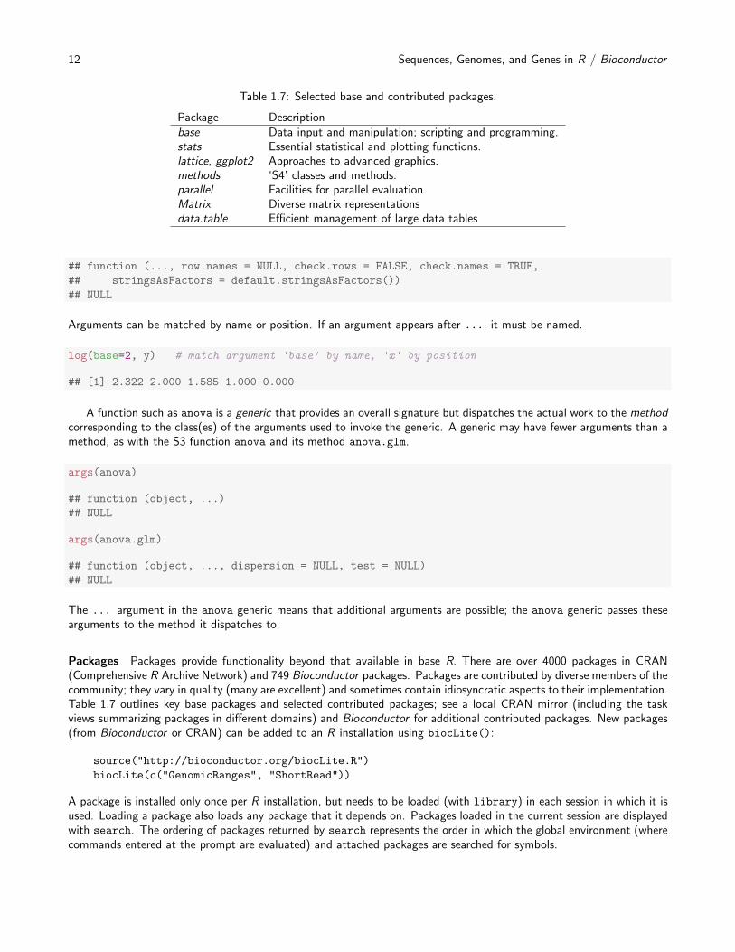
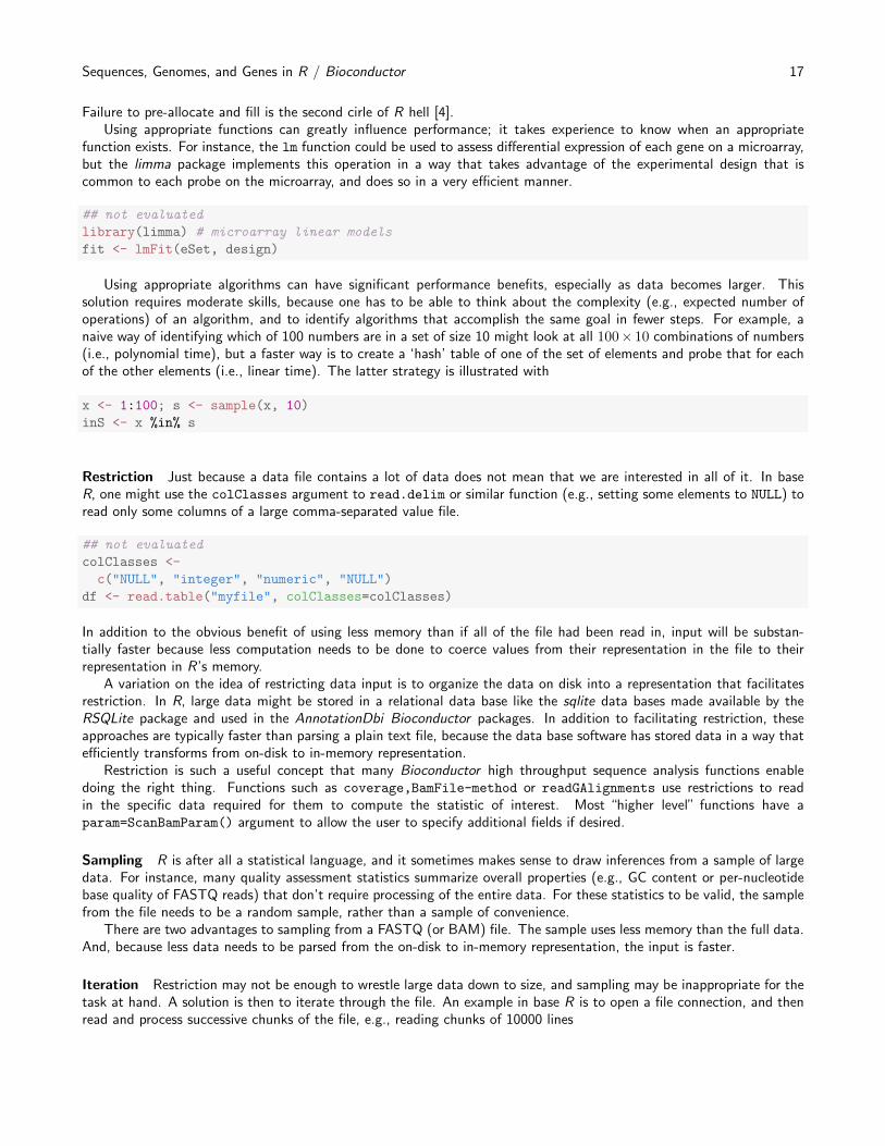