Remote Sensing of Environment 140 (2014) 580–595

Contents lists available at ScienceDirect

Remote Sensing of Environment

j ourna l homepage: www.e lsev ie r .com/ locate / rse

Separation of large scale water storage patterns over Iran using GRACE,altimetry and hydrological data

E. Forootan a,⁎, R. Rietbroek a, J. Kusche a, M.A. Sharifi b, J.L. Awange c, M. Schmidt d, P. Omondi e, J. Famiglietti f

a Institute of Geodesy and Geoinformation (IGG), Bonn University, Bonn, Germanyb Surveying and Geomatics Engineering Department, University of Tehran, Iranc Western Australian Centre for Geodesy, The Institute for Geoscience Research, Curtin University, Perth, Australiad German Geodetic Research Institute (DGFI), Munich, Germanye IGAD Climate Prediction and Applications Centre (ICPAC), Nairobi, Kenyaf UC Center for Hydrologic Modeling, University of California, Irvine, CA, USA

⁎ Corresponding author. Astronomical, Physical and MGroup, Institute for Geodesy and Geoninformation (IGG)17, D-53115, Bonn, Germany.

E-mail addresses: forootan@geod.uni-bonn.de (E. Foro(R. Rietbroek), kusche@geod.uni-bonn.de (J. Kusche), shaJ.Awange@curtin.edu.au (J.L. Awange), schmidt@dgfi.badwphilip.omondi@gmail.com (P. Omondi), jfamigli@uci.edu

0034-4257/$ – see front matter © 2013 Elsevier Inc. All rihttp://dx.doi.org/10.1016/j.rse.2013.09.025

a b s t r a c t

a r t i c l e i n f o

Article history:Received 13 June 2013Received in revised form 25 September 2013Accepted 25 September 2013Available online 23 October 2013

Keywords:GRACE-TWSSignal separationIndependent componentsTerrestrial and surface water storageGroundwaterIran

Extracting large scale water storage (WS) patterns is essential for understanding the hydrological cycle and im-proving the water resource management of Iran, a country that is facing challenges of limited water resources.The Gravity Recovery and Climate Experiment (GRACE) mission offers a unique possibility of monitoring totalwater storage (TWS) changes. An accurate estimation of terrestrial and surface WS changes from GRACE-TWSproducts, however, requires a proper signal separation procedure. To perform this separation, this studyproposesa statistical approach that uses a priori spatial patterns of terrestrial and surfaceWS changes from a hydrologicalmodel and altimetry data. The patterns are then adjusted to GRACE-TWS products using a least squares adjust-ment (LSA) procedure, thereby making the best use of the available data. For the period of October 2002 toMarch 2011, monthly GRACE-TWS changes were derived over a broad region encompassing Iran. A priori pat-terns were derived by decomposing the following auxiliary data into statistically independent components:(i) terrestrial WS change outputs of the Global Land Data Assimilation System (GLDAS); (ii) steric-corrected sur-faceWS changes of the Caspian Sea; (iii) that of the Persian andOmanGulfs; (iv)WS changes of the Aral Sea; and(v) that of small lakes of the selected region. Finally, the patterns of (i) to (v) were adjusted to GRACE-TWSmapsso that their contributions were estimated and GRACE-TWS signals separated. After separation, our results indi-cated that the annual amplitude ofWS changes over the Caspian Seawas 152mm, 101mmover both the Persianand Oman Gulfs, and 71mm for the Aral Sea. Since January 2005, terrestrial WS inmost parts of Iran, specificallyover the center and northwestern parts, exhibited a mass decrease with an average linear rate of ~15mm/yr.The estimated linear trends of groundwater storage for the drought period of 2005 toMarch 2011, correspondingto the six main basins of Iran: Khazar, Persian and Oman Gulfs, Urmia, Markazi, Hamoon, and Srakhs were−6.7,−6.1,−11.2,−9.1,−3.1, and−4.2mm/yr, respectively. The estimated results after separation agree fairly wellwith 256 in-situ piezometric observations.

© 2013 Elsevier Inc. All rights reserved.

1. Introduction

Water resource of the Islamic Republic of Iran (Iran) is under pressuredue to population growth, urbanization and its related consequences(FAO, 2009). The direct impact of the increasing population (~75millionin 2010) onwater resources resulted in increased need for freshwater inpopulated centers, while its indirect impactwas an increase in demand ofagricultural land and development of irrigation lands (e.g., Ardakani,

athematical Geodesy (APMG), University of Bonn, Nussallee

otan), roelof@geod.uni-bonn.derifi@ut.ac.ir (M.A. Sharifi),.de (M. Schmidt),

(J. Famiglietti).

ghts reserved.

2009). Sarraf, Owaygen, Ruta, and Croitoru (2005) state that thetotal water resources per capita in Iran plunged by more than 65%since 1960, and a decrease of 16% is expected by 2025. The increaseddemand for groundwater, on one hand, and the high rate of irrigationand over-exploitation of water resources in some areas, on the otherhand, are also likely to become a serious challenge for future protectionof groundwater basins of central and northern Iran (Mohammadi-Ghaleni & Ebrahimi, 2011; Motagh et al., 2008).

Since 90% of Iran is located in arid or semi-arid areas, the directrainfall is its only water recharge. This means that only 10% of thecountry receives enough rainfall to meet its need while the other muchdrier parts are heavily dependent on groundwater. Using Synthetic-Aperture Radar (SAR) data, Motagh et al. (2008) showed a land subsi-dence related to groundwater storage extractions in the central part ofIran between 1971 and 2001. Combining precipitation data with

581E. Forootan et al. / Remote Sensing of Environment 140 (2014) 580–595

measured piezometric groundwater levels, Van Camp, Radfar, Martens,andWalraevens (2012) pointed out that there is an imbalance betweenexploitation and precipitation recharge in central Iran, which has re-sulted in the decline of water storage (WS). Their study, however,was restricted to the Shahrekord aquifer (located at ~[32.3°N] and[50.9°E]).

Such conditions, therefore, justify the exploration of alternativemonitoring tools that can provide reliable information to improvewater policies. These are needed in the management of droughtand flood related impacts, as well as improving the overall watersituation in the region. Among different hydrological parameters, totalwater storage (TWS), defined as the summation of all water masses inthe Earth's storage compartments (atmosphere, surface waters, ground-water, etc.), is an important indicator of thewater cycle (Güntner, 2008).TWS changes can also be used for evaluating the past and present state ofnatural resources such as water and fodder, as well as for modeling theirfuture development within the context of human usage and climatechange (see e.g., Becker, Llovel, Cazenave, Güntner, & Crétaux, 2010;Forootan, Awange, Kusche, Heck, & Eicker, 2012; Grippa et al., 2011).

For a long time, mapping of terrestrial WS changes mainly relied onpiezometric observations, in-situmeteorologicalmeasurements, aswellas hydrological modeling approaches. Although such approaches arevery important for understanding the mechanism of water cycle, theyare limited e.g., by data inconsistencies, spatial and temporal data gapsor instrumental and human errors and oversights (Rodell et al., 2007).For Iran, specifically, most of the previous studies focused only onregional water variations (see e.g., Ghandhari and Alavi-Moghaddam,2011). Using such local studies, it is difficult to assess the large scale het-erogeneity of the terrestrial water cycle, due to the vast climate and to-pographic condition of the country (see, e.g., Section 2 and Modarres,2006). Other studies that looked at the large-scale water variations ofIran were restricted to the use of hydrological models (e.g.,Abbaspour, Faramarzi, Seyed Ghasemi, & Yang, 2009; Noory, van derZee, Liaghat, Parsinejad, & van Dam, 2011).

SinceMarch 2002, however, the Gravity Recovery and Climate Exper-iment (GRACE) is routinely providing satellite-based estimates of chang-es in TWS within the Earth's system (see e.g., Famiglietti & Rodell, 2013;Kusche, Klemann, & Bosch, 2012; Tapley, Bettadpur, Ries et al., 2004;Tapley, Bettadpur, Watkins et al., 2004; Wahr, Swenson, Velicogna, &Zlotnicki, 2004). GRACE-TWS has been used to study regional patternsof TWS changes, e.g., over Asia (e.g., Rodell, Velicogna, & Famiglietti,2009; Schnitzer et al., 2013; Shum et al., 2011), Africa (e.g., Awangeet al., 2013; Becker et al., 2010; Grippa et al., 2011), and Australia(e.g., Awange et al., 2011; Forootan et al., 2012; van Dijk, Renzullo, &Rodell, 2011). On a global scale, TWS changes are discussed e.g., inSyed, Famiglietti, Rodell, Chen, and Wilson (2008), and Forootan andKusche (2012). All these studies came to the same conclusion thatGRACE-TWS products are suitable for studying large-scale WS changeson annual and inter-annual time scales.

Studies which address TWS changes of the regions around Iran in-clude, for example, the works of Swenson and Wahr (2007) who usedsatellite altimetry (Jason1) together with GRACE monthly gravity solu-tions to analyze the WS changes of the Caspian Sea from mid 2002 to2006, and provided a multi-sensor monitoring of the sea. Avsar andUstun (2012) showed a downward linear trend of GRACE derived grav-ity changes over a region including Turkey andwest of Iran from2003 to2010. Studies of Llovel, Becker, Cazenave, Crétaux, and Ramillien (2010)and Baur, Kuhn, and Featherstone (2013) addressed the basin averagedTWS changes of the Volga River Basin (located in Russia), as well as theTigris–Euphrates region in Iraq. In the same region, Longuevergne,Wilson, Scanlon, and Crétaux (2012) evaluated water variations withinthe Tigris–Euphrates reservoirs and found a decrease of ~17km3 duringthe drought period between 2007 and 2010. In a recent study, Voss et al.(2013) showed that the pattern of the water loss is extending into thenorthwestern Iran including the Urmia Basin (see basin 3 in Fig. 1).They also reported that the strong decline of water storage was most

likely caused by groundwater depletion in this region between 2003and 2009. Our contribution extends these previous studies by lookingat the recent patterns of WS changes (from October 2002 to March2011) over the main basins of Iran.

Estimating accurate terrestrial or surface WS changes from GRACE-TWS products, however, requires a signal separation approach (e.g.,Forootan & Kusche, 2012; Schmeer, Schmidt, Bosch, & Seitz, 2012;Schmidt, Seitz, & Shum, 2008). This is due to the fact that: (a) GRACEtime-variable gravity field products exhibit correlated errors at high de-grees (e.g., Klees et al., 2008; Kusche, 2007; Swenson & Wahr, 2006)that need to be reduced; and (b) GRACE-TWS products represent amass integral which needs to be separated into their compartments,i.e. the mass variations within Earth's interior or on its surface or atmo-sphere. Regarding (a), it is common to apply a filter before computingTWS changes from GRACE time-variable gravity products (e.g.,Kusche, 2007). Nevertheless, this filtering introduces biases in themass change estimations since the mass anomalies are smeared outand moved due to the spatial filtering, known as the ‘leakage’ problem(Klees, Zapreeva, Winsemius, & Savenije, 2007; Swenson & Wahr,2002). Fenoglio-Marc, Kusche, and Becker (2006); Fenoglio-Marc et al.(2012) and Longuevergne, Scanlon, and Wilson (2010) show that theleakage is larger for regions where land meets water reservoirs suchas lakes, seas and oceans and also for small basins. To account forthese leakages, most of the previous studies focused on basin-wide ap-proaches (e.g., Baur et al., 2013; Fenoglio-Marc et al., 2006, 2012;Jensen, Rietbroek, & Kusche, 2013; Llovel et al., 2010; Longuevergneet al., 2010). However, due to the vast size of our region of study, andits varying climatic conditions (see Section 2), it is desirable to imple-ment information extractionmethods that allow the retrieval of spatial-ly varying WS changes. This capability is a feature that is usually lostwhen one applies basin-wide averaging methods.

Regarding (b), onemay assume that themain source of GRACE-TWSvariability consists of the contribution of the terrestrial and surface WSchanges (Güntner et al., 2007). We assume that the ocean and atmo-spheric mass variations have already been removed from GRACE time-variable solutions using de-aliasing products (Flechtner, 2007a,b). Thisprocedure in itself might introduce some errors in TWS estimations(see, e.g., Duan, Shum, Guo, & Huang, 2012; Forootan, Didova, Kusche,& Löcher, 2013). Estimation of this error is not considered in thispaper. For partitioning GRACE-TWS,most of the previous studies use al-timetry observations to account for the surfaceWS changes (e.g., Beckeret al., 2010; Swenson&Wahr, 2007) and hydrologicalmodels for terres-trial water changes (e.g., Rodell et al., 2007; Syed et al., 2005; vanDijk, 2011; van Dijk et al., 2011). Subsequently, GRACE-TWS signalsare compared or reduced with altimetry and/or model derived WSvalues. The accuracy of the estimation in such approaches might belimited since, for instance, altimetry observations contain relativelylarge errors over inland waters (e.g. Birkett, 1995; Kouraev et al., 2011)and hydrological models show limited skill (e.g., Grippa et al., 2011;van Dijk, 2011).

In this study, however, instead of removing those surface and terres-trial WS (respectively derived from altimetry and hydrological models)from GRACE-TWS maps, we use them as a priori information, to intro-duce the spatial patterns of surface and terrestrial WS changes. ThenGRACE-TWS signals are separated by adjusting the derived spatialpatterns to GRACE-TWS maps. For this, TWS data within a rectangularbox (between [23° to 48°N] and [42° to 63°E]) that includes Iran, is ex-tracted from each monthly GRACE-TWSmap. As mentioned before, themain source of TWS variability, within each map, consists of the contri-bution of the terrestrial and surface WS changes (Güntner et al., 2007).In our case, the surfacewater variations aremainly caused bywater res-ervoirs within the selected box e.g., the Caspian Sea, Persian and OmanGulfs, Aral Sea as well as other small lakes. Note that the effect of self-gravitational forces, other than those of surface and terrestrial WSchanges, might be considerable over the region. A discussion can befound in Appendix B.

13

24

5

6

Persian Gulf

Oman

CaspianSea

Major Basins of Iran

1) Khazar2)Persian and Oman Gulfs3)Urmia4)Markazi5)Hamoon6)Sarakhs

Percentage of totalarea of the country

10253

5273

Percentage of totalrenewable water resources

15465

2923

Number ofStations

24911910312

7

Mean ofLinear Trend

of 2003-2010

-6 mm/yr-5 mm/yr

-13 mm/yr-2.5 mm/yr-1.1 mm/yr-2.3 mm/yr

Alborz

Zagros

Fig. 1. An overview of in-situ groundwater stationswithin the sixmajor basins of Iran. The definition of the basins, their areas and renewable water resource percentages are according toFAO (2009). In-situ observations are provided by the Iranian Water-resource Research Center. The linear rate of water storage change is computed using a least squares approach, whileconsidering the annual and semi-annual frequencies. The Caspian and Aral Seas as well as the Persian and Oman Gulfs are masked out in blue.

582 E. Forootan et al. / Remote Sensing of Environment 140 (2014) 580–595

The higher-order statistical method of independent componentanalysis (ICA) (Forootan&Kusche, 2012, 2013) is used to identify statis-tically independent patterns from (i) monthlyWS outputs of the GlobalLandData Assimilation System (GLDAS)model (Rodell et al., 2004) overthe selected rectangular box; (ii) Surface WS changes derived fromaltimetry observations of Jason1&2 missions over the Caspian Sea;(iii) sea surface heights (SSHs) in the Persian and Oman Gulfs after re-moving steric sea level changes; (iv) surface WS changes in the AralSea; as well as (v) the other main lakes of the selected box. The derivedindependent patterns of (i) to (v) were used as known spatial patterns(base-functions) in a least squares adjustment (LSA) procedure, to sep-arate GRACE-TWS maps. This procedure gives the opportunity to makethe best use of all available datasets in an LSA framework. A similarargument has been pointed out e.g., in Schmeer et al. (2012), whoused experimental orthogonal functions of geophysical models in anLSA model for separating global GRACE integral signals. After separa-tion, besides adjusting the terrestrial WS of (i) to GRACE-TWS, and theestimation of surface WS changes of the region (ii to v), for the firsttime, our study offers changes of the groundwater within the six mainbasins of Iran (basins are shown in Fig. 1). Our results are also comparedwith in-situ piezometric measurements.

The remaining part of the paper is organized as follows: in Section 2,we briefly describe the study region. The data used in the study ispresented in Section 3. Section 4 outlines the analysis methods, andthe results of separation are presented anddiscussed in Section 5. Finally,Section 6 concludes the paper and provides an outlook. The paper alsoincludes two appendices that provide the results of ICA applied on

GLDAS and altimetry derived WS changes (Appendix A), and the effectof self-gravitation on the results (Appendix B).

2. The study region

2.1. Geography

Iran with an area of about 1.7millionkm2 lies between latitudes [24°to 40°N] and longitudes [44° to 64°E] (Fig. 1). The landscape of Iranis dominated by rugged mountain ranges that separate various ba-sins from each other. The largest mountain chain is that of theZagros, which runs from the northwest of the country southwardsto the shores of the Persian Gulf and then continues eastwardsalong most of the southeastern province. Alborz is the other mainmountain chain range that runs from the northwest to the eastalong the southern edge of the Caspian Sea. Over 50% of the area be-tween the two main chains is covered by salty swamps of Dasht-e-Kavir and Dasht-e-Lut.

2.2. Basins and climate

According to FAO (2009), there are 6 main catchments in Iran(i.e. Fig. 1) that include, the Central Plateau in the center (basin 4;Markazi), the Lake Urmia Basin in the northwest (basin 3), the Persianand Oman Gulf Basins in the west and south (basin 2), the Lake HamoonBasin in the east (basin 5), the Kara-KumBasin in the northeast (basin 6;Sarakhs) and the Caspian Sea Basin in the north (basin 1; Khazar). All

583E. Forootan et al. / Remote Sensing of Environment 140 (2014) 580–595

these basins, except the Persian and Oman Gulf Basin, are interior. TheMarkazi Basin, covering over half of the area of the country, has lessthan one third of the total renewable water resources (FAO, 2009).Shapes of the basins, their areas, and the percentage of their renewablewater resources are summarized in Fig. 1.

The climate of Iran is quite extreme. Its northern edge is categorizedas subtropical region (Khazar Basin in Fig. 1).Whereas the climate of theother parts, i.e. 90% of the country, ranges from arid to semiarid, withextremely hot summers in the central and southern coastal regions.The main source of the input water in Iran is annual precipitation. Thehighest annual rainfall of 2275mm has been recorded in Rasht, locatednear the Caspian Sea. Annual rainfall is less than 50mm in the deserts(FAO, 2009).

2.3. Main surface waters of the region

2.3.1. The Caspian SeaThe Caspian Sea, with an area of ~371,000km2, is theworld's largest

inlandwater body (Kosarev &Yablonskaya, 1994). Kouraev et al. (2011)provide a detailed description on the geographical and physical aspectsof the Caspian Sea. The Caspian Sea exhibits considerable fluctuationsin its water levels, which have been the subject of several studies(e.g., Kouraev et al., 2011; Sharifi, Forootan, Nikkhoo, Awange, & Najafi-Alamdari, 2013). Using a point-wise technique, Sharifi et al. (2013) illus-trated that due to the vast size of Caspian, the varying climatic patternswithin the whole sea, and the large impact of the Volga River, each re-gion of the sea is expected to have a water level pattern different fromthe other regions. The extreme temperature conditions of the sea alsocontribute to the changing of the sea level, which exhibits an annualamplitude of ~20mm (e.g., Swenson & Wahr, 2007).

2.3.2. Urmia LakeLake Urmia (located in theUrmia Basin shown in Fig. 1, ~[37.7°N and

45.31°E]) is a salty lake with a surface area of ~5000 km2 (year 2000).The area of the lake is shrinking, which is partly due to the decade-long drought of its watershed and also due to the construction of35 dams (since the 1990s) on the rivers which feed the lake.Crétaux et al. (2011) provided altimetry and imagery results forLake Urmia (e.g., http://www.legos.obs-mip.fr/en/soa/hydrologie/hydroweb/Page_2.html).

2.3.3. The Persian Gulf and the Gulf of OmanThe Persian Gulf, with a surface area of ~251,000 km2, is a shallow

water body in the south (see Fig. 1). Since the Gulf region is surroundedby arid landmasses, it has strong seasonal and even daily air temper-ature fluctuations. Air temperature can drop to 0 °C in winter andreach up to 50 °C in summer (Kampf & Sadrinasab, 2006), whichcan contribute to the level fluctuations. Long-term observations ofsea level also shows a rise at the head of the Persian Gulf, located inthe Tigris–Euphrates delta of southern Iraq and the adjacent regionsof southwestern Iran. Lambeck, Esat, and Potter (2002) linked thisrise to post-glacial rebound.

The Gulf of Oman connects the Arabian Sea to the Persian Gulf viathe Strait of Hormuz. Thewaters of the Gulf of Oman havemore oceaniccharacteristics than those of the Persian Gulf. However, this doesnot make the fluctuation of the Gulf greater than the Persian Gulf.Hydrology and circulation aspects of the Oman Gulf are discussede.g., in Pous, Carton, and Lazure (2004).

3. Data

Four main datasets for the period of 2002 to 2011 were used inthis study. These are (a) monthly TWS variations derived from GRACE,(b) surface WS changes derived from satellite altimetry observations,(c) terrestrialWS changes from GLDAS, and (d) 256 in-situ piezometricobservations covering the six main basins of Iran. In addition, maps of

sea surface temperature (Reynolds, Rayne, Smith, Stokes, & Wang,2002) and steric sea level (Ishii & Kimoto, 2009) variations are alsoused to reduce the contribution of temperature and salinity changesfrom altimetric SSHs, while converting them to surface WS changes.Note that surface WS is commonly called equivalent water height(EWH) in other studies.

3.1. GRACE

GRACE, a joint German/USA satellite project, was launched inMarch2002 to detect mass variations within the Earth's system. In this work,we examined monthly GFZ release 04 gravity field solutions providedby the German Research Centre for Geosciences (GFZ) (Flechtner,2007b). The data was computed up to degree and order 120 and coversthe period from October 2002 to March 2011. GRACE degree 1 coeffi-cients have been augmented by the results of Rietbroek et al. (2009)in order to include the variation of the Earth's center of surface figurewith respect to the Earth's center of mass, in which GRACE productshave been computed. We also replaced the zonal degree 2 sphericalharmonic coefficients (C20) by values obtained from satellite laser rang-ing (SLR) (Cheng& Tapley, 2004),whichwere obtained from theGRACETellus Team website (grace.jpl.nasa.gov).

GRACE time-variable products contain correlated errors, manifestingitself as a striping pattern (Kusche, 2007). In order to remove the stripes,we applied thede-correlationfilter of DDK2 (Kusche, Schmidt, Petrovic, &Rietbroek, 2009) to the GFZ solutions. The choice of the DDK2 filter,which is an anisotropic filter, arises from the consistent results with re-spect to the outputs of hydrological models (Werth, Güntner, Schmidt,& Kusche, 2009). Before computing monthly TWS fields, residual gravityfield solutionswith respect to the temporal average over the study periodwere computed. The residual coefficients were then transformed into0.5°×0.5° TWS maps using the approach in Wahr, Molenaar, and Bryan(1998). A rectangular box (between [23° to 48°N] and [42° to 63°E])was then extracted from the monthly TWS grids. For the region of inter-est, the gridded Root-Mean-Square (RMS) of the GRACE-TWS signals isshown in Fig. 2,A. Strong anomalies are visible over the Caspian Sea,Lake Urmia, as well as over parts of the Zagros and Alborz mountains.The large RMS of the signal over the Caspian Sea and the mountains isdue to the strong seasonality of TWS changes. Over Urmia, the strengthof the GRACE-derived storage signal is mainly due to the water loss ofthe lake (see e.g., Voss et al., 2013).

3.2. Altimetry data

Weusedmonthly gridded altimetry data over the rectangular regionmentioned above (including the Caspian Sea, the Aral Sea, the Persianand Oman Gulfs, and Urmia Lake as well as other small lakes and res-ervoirs), covering 2002 to 2011.3. Sea surface heights (SSHs) wereoriginally produced by AVISO and provided through NOAA ERDDAP(the Environmental Research Division's Data Access Program, seehttp://coastwatch.pfeg.noaa.gov/erddap/griddap/noaa_pifsc_9c36_df47_3dd4.html). The RMS of the altimetry signals is shown in Fig. 2,B. For theCaspian Sea, which has the dominant impact on the GRACE-TWS signalsover the region, we compared NOAA's SSH with the gridded results ofSharifi et al. (2013), and obtained a correlation of 0.91 for the period of2002 to 2010.

Water level fluctuations derived from altimetry can be compared toGRACE results, when they are corrected for the so-called steric or volu-metric height variations caused by temperature and salinity changes(Chambers, 2006). From the areas that contain surface water in thisstudy, the levels of the Caspian Sea and the Persian and Oman Gulfs ex-hibit a considerable steric component. We usedmonthly steric sea levelchanges of Ishii and Kimoto (2009) to convert SSH of the Persian andOman Gulfs to surface WS changes. Since Ishii and Kimoto (2009)'sstudy does not cover the Caspian Sea, we followed the approach ofSwenson and Wahr (2007) by using SST (sea surface temperature)

A) RMS of GRACE-TWSB) RMS of surface WSfrom altimetry products

C) RMS of terrestrial WSfrom GLDAS

[mm] [mm]0 100 200 0 50 100 150 0 50 100

[mm]

Fig. 2. The signal strength (RMS) of the threemaindatasets used in this study after smoothing using Kusche et al. (2009)'s DDK2filter; (A) GRACE-TWS data, (B) surfaceWS from altimetrydata and (C) terrestrial WS output of the GLDAS model.

584 E. Forootan et al. / Remote Sensing of Environment 140 (2014) 580–595

data and taking a conversion factor of 8.43 mm/yr to convert them tosteric sea level changes over the Caspian Sea. The SST data, usedhere, were reconstructed Reynolds et al. (2002) SST maps obtainedfrom the United States (US) National Oceanic and Atmospheric Ad-ministration (NOAA) official website (http://www.esrl.noaa.gov/psd/data/gridded/data.ncep.oisst.v2.html). Each map of SSH (afterreducing the steric part) was filtered using the same DDK2 filter asapplied to the GRACE-TWS maps. After applying the DDK2 filter onsurface WS data, the mean damping ratio of the filtered data to theoriginal values was ~0.71.

3.3. GLDAS model

The GLDAS hydrological model integrates a large quantity of ob-served data and modeling concepts (Rodell et al., 2004) to produce aglobal hydrological model. GLDAS terrestrial WS data for the period ofstudy were obtained from the Goddard Earth Sciences Data and Infor-mation Services Center (http://grace.jpl.nasa.gov/data/gldas/). Conse-quently, terrestrial WS considered here constitutes of total columnsoil moisture (TSM), snow water equivalent (SWE) and canopy waterstorage (CWS). Groundwater storage changes are not represented inthe GLDASmodel simulations. As a result, our a priori pattern of the ter-restrial storage partitioning is limited, andmight not include a completedescription of the lateral and vertical distribution of water storage up tothe surface (see e.g., Rodell & Famiglietti, 2001; Syed et al., 2008). TheGLDAS-WS data were filtered by the same DDK2 filter in order tomatch the signal content of the GRACE-TWS fields. The RMS of GLDASdata for the mentioned rectangular box is shown in Fig. 2,C. The resultsshow strong signals over the northwest of the country and over theZagros and Alborz mountains. The strength of the signal is due to thestrong annual variability of TWS over these regions. We compared themean magnitude of the DDK2-filtered GLDAS data with its originalvalues over the region and found a damping ratio of ~0.83 due to thefilter.

3.4. In-situ piezometric measurements

This study used in-situ groundwater observations of 256 selectedpiezometric stations of the Iranian Water-resource Research Center, ofwhich 24, 91, 19, 103, 12 and 7 stations are located in the basins 1 to6 of Fig. 1, respectively. The observations cover the period 2003 to2010 and have been tested for their quality in terms of outliers and pos-sible biases. The location of the stations and their computed linear

trends for 2003 to 2010 are shown in Fig. 1. In agreement with theother data, most parts of Iran exhibited a WS decline during the men-tioned period. Note that, there jumps exist in the in-situ time series asa result ofwater network changes. Their impact on the computed trendswill be addressed in Section 5.2.

4. Methodology

Monthly GRACE-TWS maps, used in this study (ocean and atmo-sphericmass variations are already removed), reflect an integralmeasureof the combined effect of terrestrial WS changes of land hydrology (H),and surface WS changes of seas, lakes and reservoirs (R). Assuming thatGRACE-TWS fields are stored in a matrix T=T(s,t), where t is the time,and s stands for spatial coordinate (grid points). T can be factorized intospatial and temporal components (Schmeer et al., 2012) as

T ¼ CHATH þ CRA

TR; ð1Þ

whereCH/R=CH/R(t) andAH/R=AH/R(s) are respectively the temporal andspatial patterns (base-functions).We usedH and R as subindices to showthe base-functions that are computed from terrestrialWS (H) and surfaceWS (R). In Eq. (1), CH contains zero over the grid points of surface waterand CR contains zeros over the land.

In Eq. (1), once either of CH/R(t) or AH/R(s) is determined, the othercomponent can be computed by solving an LSA. Schmeer et al. (2012)used a similar approach for separating global GRACE-TWS integralinto its atmospheric, hydrologic and oceanic contributors. Their studysuggests the application of a statistical decomposition method on thedata/model of each compartment to compute the required base-functions of Eq. (1). Accordingly, we follow their approach and usesteric corrected SSHs and the WS output from the GLDAS model asdescribed in Section 3 to compute the required CH/R and AH/R.

ICA, an extension of the second-order statistical method of principalcomponent analysis (PCA) (Preisendorfer, 1988), allows the extractionof statistically independent patterns from spatio-temporal datasets(Cardoso & Souloumiac, 1993). The applications of ICA for filtering(Frappart et al., 2010) and decomposition of GRACE-TWS are discussede.g., in Forootan and Kusche (2012, 2013) and Forootan et al. (2012). Ofthe two alternative ways of applying ICA, in which either temporallyindependent components or spatially independent components areconstructed (Forootan & Kusche, 2012), we used temporal ICA. Themotivation of this selection was based on the intentions of the study,which focuses on signals which have distinct temporal behavior

A) Lake Urmia

B) Caspian Sea

GRACE-TWS after removing GLDAS-WSGRACE-TWS

Altimetry derived surface WS

Fig. 3. SurfaceWS changes derived fromGRACE and altimetry data, for (A) Lake Urmia and(B) the Caspian Sea. For computing the volume (y-axis), the mean surface area of theCaspian Sea and Urmia Lake (Section 2.3) is multiplied by the mean columnsWS changesderived from GRACE and altimetry. During the computations, the shrinking area of LakeUrmia is also taken into account (see also Crétaux et al., 2011).

585E. Forootan et al. / Remote Sensing of Environment 140 (2014) 580–595

(e.g., seasonal and trend of water changes). The temporal ICAmethod issimply called ICA in this paper, and the decomposition of the centered(temporal mean removed) time series of H and R is written as

H ¼ PHRHRTHE

TH ¼ CHAH

T; ð2Þ

and

R ¼ PRRRRTRE

TR ¼ CRAR

T: ð3Þ

As stated in Forootan and Kusche (2012), PH=R and EH/R containorthogonal components in their columns that are derived by applyingPCA on the centered datasets of H and R (Preisendorfer, 1988). InEqs. (2) and (3), T is a transpose operator, PH=R is normalized (i.e. PH=R

PTH=R ¼ I), RH=R is an optimum rotation matrix that rotates the temporal

components ofPH=R to make them temporally as mutually independentas possible (Forootan & Kusche, 2012).

As a result of the temporal ICA decomposition, CH=R ¼ PH=RRH=R

contains statistically mutually independent temporal components.AH=R ¼ EH=RRH=R stores their corresponding spatial maps, that are stillorthogonal. AH/R, therefore, will be used in Eq. (1) as known spatialpatterns and a new temporal expansion of CH=R will be computedusing the LSA approach (e.g., Koch, 1988),

CH CR

h iT ¼ AH AR½ �T AH AR½ �h i−1

AH AR½ �TTT: ð4Þ

In Eq. (4), CH=R contains adjusted temporal components over the landand surface waters and T contains GRACE-TWS observations. Then, CH

and CR can be respectively replaced in Eqs. (2) and (3) to reconstruct ter-restrial WS changes over the land and surface WS changes.

5. Numerical results

5.1. Comparison of GRACE and altimetry

From Fig. 2,A, the strongest variability during 2002–2011 detectedby GRACE is concentrated over Urmia Lake and the Caspian Sea. Beforeimplementing the separation approach described in Section 4, we firstcompared the averaged volume variations of Urmia and the CaspianSea derived from GRACE with those of satellite altimetry. For deriv-ing the time series of the Urmia Basin, we took the boundary ofbasin 3 in Fig. 1 as our reference. A basin-averaged TWSwas comput-ed for Urmia Lake using a similar approach to that of Swenson andWahr (2007), which is the dash-black line in Fig. 3,A. Then, the con-tribution of terrestrial WS surrounding Urmia Lake was removedfrom GRACE-TWS using GLDAS data, which is shown as the solid-black line in Fig. 3,A. Our result of surface WS changes from GRACE iscomparable, in terms of cycles and trend, with those of Crétaux et al.(2011) for Lake Urmia (the solid-gray line in Fig. 3,A), derived fromaltimetry and imagery products (http://www.legos.obs-mip.fr/soa/hydrologie/hydroweb/StationsVirtuelles/SV_Lakes/Urmia.html).

WS change of the Caspian Sea from GRACE products is shown bythe solid-black line in Fig. 3,B. For computing the averaged surface WSchanges over the Caspian Sea, the average value of steric correctedSSHs was multiplied by the surface area of the sea and is shown bythe solid-gray line in Fig. 3,B. The correlation coefficient between thetwo curves is 0.81, at 95% confidence level, indicating a good agreement.However, in some years (e.g., 2004 and 2008), there are observabledifferences between the estimated amplitude of the annual WS signalfrom GRACE and altimetry. This could be due to the steric correctionor due to the errors in altimetry data itself. Such observed inconsis-tencies motivated the introduced approach for separating GRACE-TWSsignals.

5.2. Separation (adjustment) results

The RMS of GRACE-TWS signals in Fig. 2,A clearly demonstrates theleakage problem. For instance, a part of the Caspian Sea's WS leakedinto its surrounding terrestrial signal or vice versa. In order to separateGRACE-TWS changes, we first extracted independent components ofWS changes from altimetry and GLDAS outputs. The results are shownand described in Figs. A1, A2, A3, A4 and A5 of Appendix A. The spatialpatterns of the mentioned figures were postulated as known patternsin Eq. (4). We also added four other independent components fromGLDAS data to Eq. (4). Note that, in order to restrict the length of thepaper, patterns of IC3 to IC6 are not shown in Appendix A. The adjustedtemporal patterns of surface and terrestrial WS changes are computedusing Eq. (4) and are shown in Figs. 4 and 5, respectively. In thispaper, the temporal components are scaled by their standard deviationsto be unit-less. Spatial patterns of the figures in Appendixes A and B arescaled by the standard deviations of their corresponding temporal com-ponents to represent anomaly maps of WS in millimeter.

From the annual patterns of surfaceWS changes, i.e. Fig. 4,A, C, E andF, the amplitude of the adjusted signals is comparable to those of altim-etry derived surfaceWS (EWH) changes. Comparing the adjusted inter-annual changes of surfaceWS changes (the black lines in Fig. 4,B and D)

IC 1 of the Caspian Sea-EWH Adjusted-EWH Altimetry EWH

IC 2 of the Caspian Sea-EWH

IC 1 of the Persian and Oman Gulfs-EWH

IC 1 of the Aral Sea-EWH

IC 1 of the small lakes-EWH

2002 2003 2004 2005 2006 2007 2008 2009 2010 2011-2

0

2

2002 2003 2004 2005 2006 2007 2008 2009 2010 2011

-2

0

2

2002 2003 2004 2005 2006 2007 2008 2009 2010 2011-2

0

2

A)

B)

C)

2002 2003 2004 2005 2006 2007 2008 2009 2010 2011

-2

0

2

D)

E)

F)

IC 2 of the Persian and Oman Gulfs-EWH

Adjusted-EWH Altimetry EWH

Adjusted-EWH Altimetry EWH

Adjusted-EWH Altimetry EWH

Adjusted-EWH Altimetry EWH

Adjusted-EWH Altimetry EWH

2002 2003 2004 2005 2006 2007 2008 2009 2010 2011

-2

0

2

2002 2003 2004 2005 2006 2007 2008 2009 2010 2011-2

0

2

Fig. 4. An overview of the adjusted and altimetry derived surfaceWS changes, shown here in equivalent water height (EWH). The red lines are derived using the LSAmethod of Section 4and the black lines are derived from the ICA decomposition of altimetry derived surface WS changes (see Appendix A). (A,B) the first two independent components of theCaspian Sea; (C,D) the first two independent components of the Persian and Oman Gulfs; (E) the first independent component of the Aral Sea; and (F) the first independent componentof the small lakes. The temporal patterns are unit-less. The corresponding spatial patterns of (A,B) are shown in Fig. A1; those of (C,D) in Fig. A2; the spatial pattern of (E) in Fig. A3; andthat of (F) in Fig. A4. The independent modes are ordered with respect to the variance fraction they represent.

586 E. Forootan et al. / Remote Sensing of Environment 140 (2014) 580–595

to their altimetry-derived estimates (the red lines in Fig. 4,B and D)shows that the adjusted values (i.e. coming from GRACE products) aresmoother compared to the altimetry results. This is also true for theannual component of the Aral Sea (compare the red and black lines inFig. 4,E). Investigating the reason for this difference may be the subjectof future research.

From the adjusted results, we estimate the amplitude of annual sur-faceWS changes of the Caspian Sea to be 150mm, whereas amplitudesof 101mm and 71mm are obtained for the Persian and Oman Gulfs, re-spectively. Fig. 4,E indicates a negative linear trend of ~20mm/yr during2002 to 2011 over the Aral Sea.

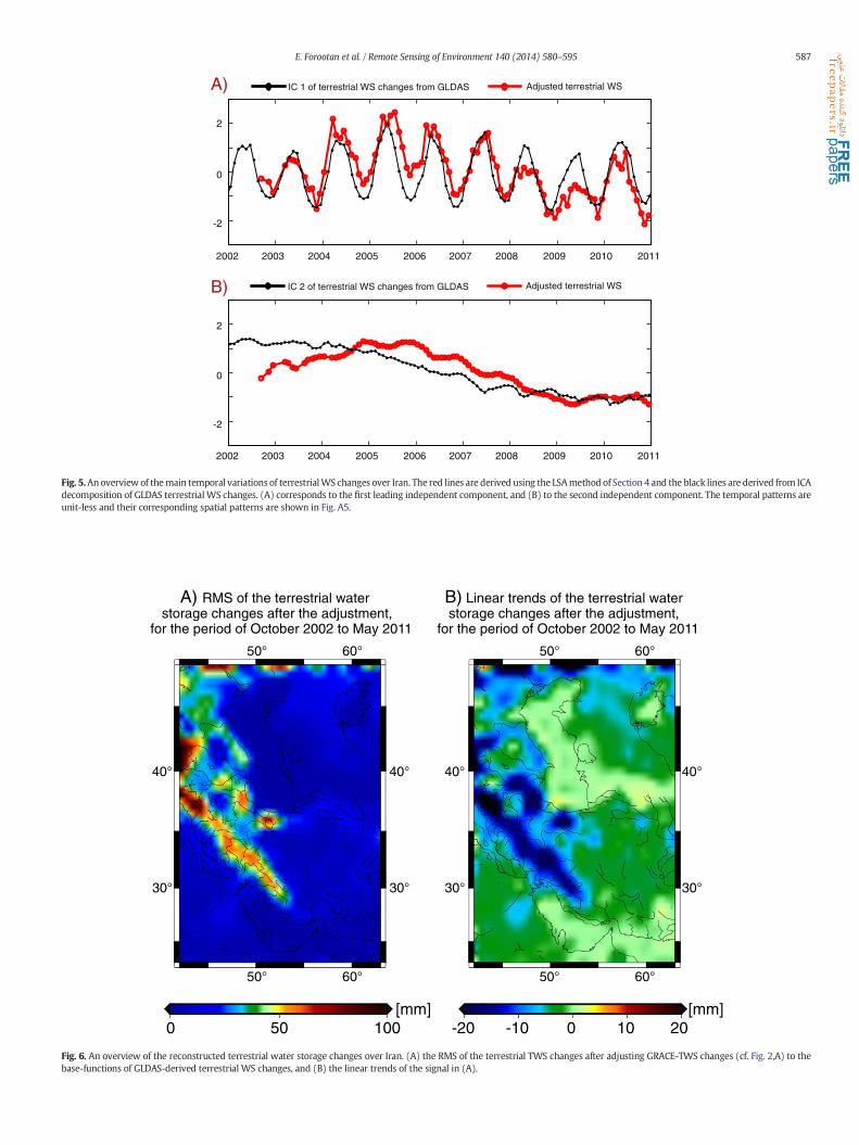
IC1 in Fig. 5,A compares the adjusted value of annual terrestrial WSchangeswith theWSoutput of GLDAS. Although, the phase of the signalis comparable, the amplitudes of the signal differ over the years. For in-stance, an attenuation of the annual amplitudes in the years 2008 and2009, derived from GRACE (the red line in the temporal pattern ofIC1), could be related to the prolonged drought condition over Iran(Shean, 2008). This impact is not fully reflected in the GLDAS outputs(the black line in Fig. 5,A). IC2 of GLDAS (the black line in Fig. 5,B)shows an overall decline of terrestrial WS changes mainly over the cen-tral and north-western parts of Iran (see the spatial map of IC2 inFig. A5). The adjusted value of IC2 (the red line in Fig. 5,B) shows that

the drought trend actually starts from 2005. The adjusted results aremore consistent with the drought behavior we found for the smalllakes of the country and also in-situ observations, with all showing adecline after 2005. We estimate an average decline of 15mm/yr watercolumn during 2005 to 2011 over central Iran.

5.3. Comparison of the adjusted results with in-situ observations

Once the signals of the surface and terrestrialWS changes have beenseparated and their amplitudes are adjusted to the GRACE observations,we use the spatial base-functions derived from GLDAS (i.e. spatial mapsof Fig. A5 and 4 other maps that are not shown in the paper) alongwiththeir corresponding adjusted temporal values (the red lines in Fig. 5and 4 others) in Eq. (2) to reconstruct terrestrial WS changes overIran. In Eq. (2), the spatial maps stored in AH and CH contain the ad-justed temporal components. The RMS and linear trends of the re-constructed signals are shown in Fig. 6,A and B, respectively. TheRMS shows that the separation was successful, where for example,the leakage caused by the Caspian Sea signal is removed (compareFig. 6,A with Fig. 2,A). The linear trends (Fig. 6,B) show a decline inmost parts of the country including the northwest, central, as wellas over the Zagros chain.

IC 1 of terrestrial WS changes from GLDAS Adjusted terrestrial WS

2002 2003 2004 2005 2006 2007 2008 2009 2010 2011

-2

0

2

A)

B)

2002 2003 2004 2005 2006 2007 2008 2009 2010 2011

-2

0

2

IC 2 of terrestrial WS changes from GLDAS Adjusted terrestrial WS

Fig. 5.An overview of themain temporal variations of terrestrialWS changes over Iran. The red lines are derived using the LSAmethod of Section 4 and the black lines are derived from ICAdecomposition of GLDAS terrestrial WS changes. (A) corresponds to the first leading independent component, and (B) to the second independent component. The temporal patterns areunit-less and their corresponding spatial patterns are shown in Fig. A5.

50°

50°

60°

60°

30° 30°

40° 40°

[mm]

50°

50°

60°

60°

30° 30°

40° 40°

-20 -10 0 10 200 50 100[mm]

A) RMS of the terrestrial waterstorage changes after the adjustment,

for the period of October 2002 to May 2011

B) Linear trends of the terrestrial waterstorage changes after the adjustment,

for the period of October 2002 to May 2011

Fig. 6. An overview of the reconstructed terrestrial water storage changes over Iran. (A) the RMS of the terrestrial TWS changes after adjusting GRACE-TWS changes (cf. Fig. 2,A) to thebase-functions of GLDAS-derived terrestrial WS changes, and (B) the linear trends of the signal in (A).

587E. Forootan et al. / Remote Sensing of Environment 140 (2014) 580–595

588 E. Forootan et al. / Remote Sensing of Environment 140 (2014) 580–595

We removed the above reconstructed results from GRACE-TWSmaps and compared the results with available in-situ groundwater ob-servations. Before, comparison, eachmonth of the available stationswasfirst smoothed using a Gaussian filter of 400 km radius (Jekeli, 1981).The radius of 400 km was selected to be approximately consistentwith the DDK2 filter applied to GRACE-TWS data. We compared themagnitude of the basin averages of the filtered in-situ observationswith those we derived from the original values (in Fig. 1). We found a

Linear trend

In-situ observations

2003 2004 2005 2006 2

-50

0

50

Kha

zar

[mm

]

2003 2004 2005 2006 2-50

0

50

Urm

ia [m

m]

2003 2004 2005 2006 2

-50

0

50

Gul

fs [m

m]

2003 2004 2005 2006 2-20

0

20

Mar

kazi

[mm

]

2003 2004 2005 2006 2-20

0

20

Ham

oon

[mm

]

2003 2004 2005 2006 2-50

0

50

Y

Sar

akhs

[mm

]

Fig. 7. Basin averages of groundwater changes over the six major basins of Iran. The red linesGRACE-TWS. The blue dashed lines are derived from in-situ piezometric observations that arenot exhibit network changes. Linear trends are shown by the black lines and their rates are rep

mean damping factor of ~0.71, which shows the impact of the GRACE-like post-processing on the true in-situ signals. A comparison of theresults is shown in Fig. 7. The basin averages derived from both in-situand satellite observations are consistent in terms of the seasonal peaksand phases. The linear rates of the water storage changes are depictedin Fig. 7 (dash lines). As the figure illustrates, in most of the basins,GRACE derived basin averages tend to show steeper slopes comparedto the in-situ observations. Part of this inconsistencymight be the result

GRACE derived groundwater storage after reducing the adjusted GLDAS

In-situ observations

007 2008 2009 2010 2011

007 2008 2009 2010 2011

007 2008 2009 2010 2011

007 2008 2009 2010 2011

007 2008 2009 2010 2011

007 2008 2009 2010 2011

ear

are basin averages after removing the adjusted terrestrial and surface WS changes fromlocated in each basin, respectively. Solid gray lines are derived from the stations that doorted in Table 1.

589E. Forootan et al. / Remote Sensing of Environment 140 (2014) 580–595

of network changes in a number of stations. We removed those stationsfrom our basin average computations and the new results turned out tobemore consistent with that of GRACE (solid gray lines). The other partof inconsistency might be due to our limited knowledge about the po-rosity parameters used for converting piezometer observations to stor-age values, which can be quite large for some basins (see e.g., Jiménez-Martínez et al., 2013). Further research, e.g., involving permanentGPS stations, needs to be undertaken to address the problem over theselected region. The results of GRACE-derived groundwater rates aresummarized in Table 1.

6. Conclusion and outlooks

The water resources in Iran as a part of the Middle-East region areinherently scarce as a result of naturally arid climatic conditions. Popu-lation increase and economic growth have spurred higher demands forthe limited water resources (FAO, 2009). Therefore, it is desirable todevelop monitoring and analysis tools to aid understanding the hydro-logical cycle of the region. In this context, this study investigated largescale GRACE-TWS pattern changes over a rectangular region that in-cluded Iran for the period from October 2002 to March 2011. The ex-tracted patterns are important since GRACE-TWS changes representintegral measurements of water in the entire region. Spatio-temporalchanges of TWS, therefore, may be used to study natural and man-madeimpacts on the regional climate.

In order to deal with the leakage problem of GRACE products andalso to separate terrestrial from surfaceWS changes, a least squares ad-justment approach was applied on the ICA-decomposed terrestrial andsurface WS variations respectively from GLDAS and altimetry WS out-puts. The appliedmethod only relies on the ICA-derived spatial patternsof the hydrological model and altimetry observations, which remain in-variant in the adjustment. In the adjustment step, the temporal compo-nents are estimated from GRACE-TWS data (Section 5.2). Adjustedterrestrial WS over Iran showed an overall declining trend over thecountry (Fig. 6,B). In Section 5.3, we demonstrated that the estimatedgroundwater storages are in a good agreementwith in-situ piezometricobservations. Furthermore, for the first time, this study offers GRACE-derived basin averaged groundwater changes for the six main basinsof Iran (basins are selected according to FAO, 2009). Our estimates ofthe linear trends of WS changes for the period of 2003 to 2005 andthe drought period of 2005 to 2011.3 are shown in Table 1. In view ofthe low availability of renewable water resources in all the basins, inparticular, the Markazi and Urmia Basins, the results may be an impor-tant incentive for thewater resourcemanagement of Iran. Note that thearea of some of our processed basins, for instance Urmia and Sarakhs,is relatively small and might not meet the nominal resolution of theGRACE-TWS products. However, the strong WS signal of the basins andtheproposed optimal processingmethod allowed retrieval ofwater stor-age variations.

At the root of the presented separation procedure lies in the ICA-decomposition of the GLDAS and altimetry outputs. Such decomposi-tions contain errors as a result of the short length of observations, aswell as the errors of observations themselves. Including those errors inthe least squares procedure may potentially improve the results butfall outside the scope of the current research. The performed separationapproach has the potential to be improved by adding extra information

Table 1Basin average trends of groundwater variations over the six main basins of Iran derived from G

Basins: Khazar(Basin 1)

Gulfs(Basin 2)

Groundwater rate of 2003–2005 [mm/yr]: 8.6 5.1Groundwater rate of 2005–2011 [mm/yr]: −6.7 −6.1

on the patterns of water storage variations over the Mesopotamiaregion, which covers the Tigris/Euphrates River system, Lake Van etc.,(see e.g., Voss et al., 2013). The contribution of such base-functions inthe inversion will, however, be marginal and concentrated over thebasins located at the west part of the country (i.e. basins 2 and 3). Therelationship between WS changes in the six major basins of Iran andclimate variability such as decadal rainfall anomalies and large scaleocean-atmospheric patterns of e.g., the El Niño Southern Oscillationphenomenon might be helpful for understanding the water cycle ofthe region.

Acknowledgment

The authors thank the editor M. Bauer and the anonymous reviewerfor the helpful remarks, which improved the manuscript considerably.E. Forootan and J. Kusche are grateful for the financial support providedby the German Research Foundation (DFG) under the project BAYES-G.E. Forootan thanks L. Moxey (the Operations Manager of NOAA OceanWatch — Central Pacific) for the fruitful discussions on altimetry of theCaspian Sea. He also thanks L. Longuevergne (Université de Rennes1) for his useful comments on theperformed investigations. The authorsalso thank Y. Hemmati (Iranian Water-resource Research Center) forproviding the in-situ observations. We are grateful for the satellite andmodel data used in this study. This is a TIGeR Publication no. 491.

Appendix A. Extracting independent components from GLDAS andaltimetry WS changes

ICA is applied on the datasets on each GLDAS and altimetry datasetsusing Eqs. (2) and (3) (see the details of application in e.g., Forootan &Kusche, 2012). For altimetry products, ICAwas individually implement-ed on (i) the Caspian Sea, (ii) the Persian and Oman Gulfs, (iii) the AralSea, and finally (iv) the other small lakes. The results are depicted inFigs. A1, A2, A3 and A4. Note that, similar to the main text, all the tem-porally independent components (ICs) are unit-less and the spatialpatterns are given in millimeters.

Fig. A1 shows the first two independent modes, accounting for 93%of the surface WS variance in the Caspian Sea. The remaining 7% of thevariance is noisy and is not shown here. IC1 shows an annual behavioralong with two linear trends, one from January 2002 to December2005 with a rate of 108 mm/yr and the other from January 2006 toOctober 2008 with a rate of −152 mm/yr. IC2 indicates the maininter-annual variability from which, the spatial pattern of IC2 showsthat the northern part of Caspian exhibits stronger inter-annual varia-tions compared to the central and southern parts (see Fig. A1). Thiscan be related to the climatic extremes, which are more pronouncedin the northern part of the Caspian Sea inducing stronger mass varia-tions (Kouraev et al., 2011; Sharifi et al., 2013).

The ICAdecomposition ofWS changes of the Persian andOmanGulfsalso shows two significant components explaining 89% of the totalvariance. IC1 shows an annual behavior with a dipole spatial struc-ture over the two gulfs (see Fig. A2, spatial pattern of IC1). IC2shows a superposition of inter-annual variability and a positive line-ar trend (9 mm/yr) dominant mainly over the head of the PersianGulf, where Lambeck et al. (2002) reported a rise due to the post-glacialrebound.

RACE products.

Urmia(Basin 3)

Markazi(Basin 4)

Hamoon(Basin 5)

Sarakhs(Basin 6)

8.5 2.5 1.3 3.7−11.2 −9.1 −3.1 −4.2

Spatial pattern of IC 1 Spatial pattern of IC 2

10.8 cm/year -15.2 cm/yearRate (Jan.2002 to Dec-2005): Rate (Jan.2006 to Jan-2011):

2003 2005 2007 2009 2011-3

-2

-1

0

1

2

3

2003 2005 2007 2009 2011-3

-2

-1

0

1

2

3

Fig. A1. Results of the ICA method applied to the steric corrected SSH data (surface WS changes) over the Caspian Sea. The results are ordered according to their signal strength.

590 E. Forootan et al. / Remote Sensing of Environment 140 (2014) 580–595

Fig. A3 shows that only one of the independent component ofsurface WS changes (corresponding to 89% of the total variance) overthe Aral Sea is statistically significant. IC1 of Aral shows the shrinkingof the sea with an average linear rate of 300 mm/yr. Results of ICA,applied on surface WS changes of the small lakes and reservoirs, areshown in Fig. A4. While only the first IC corresponding to 93% of totalvariance was significant, it shows that most of the surface waters ofIran, specifically after the year 2005, are losing water. This situationmight be related to the long-term drought condition of the country(see e.g. Bari-Abarghouei, Asadi-Zarch, Dastorani, Kousari, and Safari-Zarch, 2011).

For brevity we only present the first two independent componentsof GLDAS data, explaining 71% of the total variance of terrestrial WSchanges in Fig. A5. The temporal pattern of IC1 shows the dominant an-nual variation, while the spatial pattern of IC1 is mainly concentratedover north and west Iran. The temporal pattern of IC2 shows an overalllinear trend (during 2002 to 2010) corresponding to a decrease of WSover the Markazi and Urmia Basins (see Fig. A5, spatial pattern of IC2).The derived trend appears to differ from the observations ofWS changes,

e.g., over Urmia (Fig. 3,A) and other small lakes (Fig. A4), where the WSdecrease starts from 2005.

We should mention here, that to reconstruct 90% of the GLDAS data,one needs to select at least the first six independent components ofGLDAS. The temporal behaviors of the remaining four independentcomponents of GLDAS were difficult to interpret and are therefore notplotted. These components were, however, still used in the adjustmentprocedure.

Appendix B. Self-gravitational impact

The strong seasonal mass fluctuations in the Caspian Seawill cause atime variable change in the geoid. On very short time scales (typicallydays), the ocean will adapt itself to this new equipotential surface, sim-ilar to the tidal response of the ocean. This implies that the sea level inthe Gulfs and the Black Sea are (indirectly) influenced by the variationsin the Caspian Sea. This effect is known as the self-consistent sea levelresponse and has already been described in Farrell and Clark (1976).When unaccounted for, this effect may potentially mix signal between

Spatial pattern of IC 1

Spatial pattern of IC 2

Rate(Jan.2002 to Jan.2011):0.9 cm/year

2003 2005 2007 2009 2011-3

-2

-1

0

1

2

3

2003 2005 2007 2009 2011-3

-2

-1

0

1

2

3

Fig. A2. Results of the ICAmethod applied to the steric corrected SSH data (surfaceWS changes) over the Persian andOmanGulfs. The results are ordered according to their signal strength.

591E. Forootan et al. / Remote Sensing of Environment 140 (2014) 580–595

the base-functions discussed in themain text. We, therefore, quantifieditsmagnitude by taking the steric corrected sea level from altimetry andcomputed the self consistent sea level response according to Rietbroek,Brunnabend, Kusche, and Schröter (2012). Fig. B1 shows the RMS of this

-

-

Spatial pattern of IC1

60

60

45 45

Fig. A3. The dominant independent mode

effect. The effect is strongest in the Black Sea, since it is located closest tothe Caspian Sea. However themagnitude of the effect is very small com-pared to the hydrological and oceanic signal sought such that it is notexpected to influence the results.

2003 2005 2007 2009

2

1

0

1

2

2011

Rate (Jan. 2002 to Jan.2011)4.5 cm/year

of surface WS changes of the Aral Sea.

2003 2005 2007 2009 2011-3

-2

-1

0

1

2

3

Fig. A4. Results of the ICA method applied to the surface WS data over small lakes andreservoirs of the region.

592 E. Forootan et al. / Remote Sensing of Environment 140 (2014) 580–595

References

Abbaspour, K. C., Faramarzi, M., Seyed Ghasemi, S., & Yang, H. (2009). Assessing the im-pact of climate change on water resources in Iran. Water Resources Research, 45,W10434. http://dx.doi.org/10.1029/2008WR007615.

Ardakani, R. (2009). Overview of water management in Iran. Proceeding of regional centeron urban water management, Tehran, Iran.

Avsar, N.B., & Ustun, A. (May 6–10). Analysis of regional time–variable gravity usingGRACE's 10-day solutions. FIG working week 2012, knowing to manage the territory,protect the environment, evaluate the cultural heritage, Rome, Italy (http://www.fig.net/pub/fig2012/papers/ts04b/TS04B_avsar_ustun_5724.pdf. (accesseddate: May 2013))

Awange, J. L., Fleming, K. M., Kuhn, M., Featherstone, W. E., Heck, B., & Anjasmara, I.(2011). On the suitability of the 4° × 4° GRACE mascon solutions for remote sensingAustralian hydrology. Remote Sensing of Environment, 115, 864–875. http://dx.doi.org/10.1016/j.rse.2010.11.014.

Awange, J., Forootan, E., Kusche, J., Kiema, J. K. B., Omondi, P., Heck, B., et al. (2013). Un-derstanding the decline of water storage across the Ramser-Lake Naivasha usingsatellite-based methods. Advances in Water Resources, 60, 7–23. http://dx.doi.org/10.1016/j.advwatres.2013.07.002.

Bari-Abarghouei, H., Asadi-Zarch, M.A., Dastorani, M. T., Kousari, M. R., & Safari-Zarch, M.(2011). The survey of climatic drought trend in Iran. Stochastic EnvironmentalResearch and Risk Assessment, 25(6), 851–863. http://dx.doi.org/10.1007/s00477-011-0491-7.

Baur, O., Kuhn, M., & Featherstone, W. E. (2013). Continental mass change from GRACEover 2002–2011 and its impact on sea level. Journal of Geodesy, 87(2), 117–125.http://dx.doi.org/10.1007/s00190-012-0583-2.

Becker, M., Llovel, W., Cazenave, A., Güntner, A., & Crétaux, J. -F. (2010). Recent hydrolog-ical behavior of the East African great lakes region inferred from GRACE, satellitealtimetry and rainfall observations. Comptes Rendus Geoscience, 342(3), 223–233.http://dx.doi.org/10.1016/j.crte.2009.12.010.

Birkett, C.M. (1995). The global remote sensing of lakes, wetlands and rivers for hydrolog-ical and climate research. Geoscience and remote sensing symposium, 1995. IGARSS 95.Quantitative remote sensing for science and applications, vol. 3. (pp. 1979–1981).

Cardoso, J. F., & Souloumiac, A. (1993). Blind beamforming for non-Gaussian signals. IEEEproceedings (pp. 362370) (doi: 10.1.1.8.5684).

Chambers, D. P. (2006). Observing seasonal steric sea level variations with GRACE andsatellite altimetry. Journal of Geophysical Research, 111, C03010. http://dx.doi.org/10.1029/2005JC002914.

Cheng, M., & Tapley, B.D. (2004). Variations in the Earth's oblateness during the past28 years. Journal of Geophysical Research, 109, B09402. http://dx.doi.org/10.1029/2004JB003028.

Crétaux, J. -F., Jelinski, W., Calmant, S., Kouraev, A., Vuglinski, V., Bergé Nguyen, M., et al.(2011). SOLS: A lake database to monitor in near real time water level and storagevariations from remote sensing data. Journal of Advanced Space Research, 1497–1507.http://dx.doi.org/10.1016/j.asr.2011.01.004.

Duan, J., Shum, C. K., Guo, J., & Huang, Z. (2012). Uncovered spurious jumps in the GRACEatmospheric de-aliasing data: Potential contamination of GRACE observed masschange. Geophysical Journal International, 191, 83–87. http://dx.doi.org/10.1111/j.1365-246X.2012.05640.x.

Famiglietti, J. S., & Rodell,M. (2013).Water in the balance. Science, 340(6138), 1300–1301.http://dx.doi.org/10.1126/science.1236460.

FAO (2009). FAO water report, 34, .Farrell, W. E., & Clark, J. A. (1976). On postglacial sea level. Geophysical Journal of the Royal

Astronomical Society, 46(3), 647–667.Fenoglio-Marc, L., Kusche, J., & Becker, M. (2006). Mass variation in theMediterranean Sea

from GRACE and its validation by altimetry, steric and hydrologic fields. GeophysicalResearch Letters, 33(19). http://dx.doi.org/10.1029/2006GL026851.

Fenoglio-Marc, L., Rietbroek, R., Grayek, S., Becker, M., Kusche, J., & Stanev, E. (2012).Water mass variation in the Mediterranean and Black Sea. Journal of Geodynamics,59–60, 168–182. http://dx.doi.org/10.1016/j.jog.2012.04.001.

Flechtner, F. (2007a). AOD1B product description document for product releases 01 to 04.Technical report. Potsdam: Geoforschungszentrum (GFZ).

Flechtner, F. (2007b). GFZ Level-2 processing standardsdocument for level-2product release0004, GRACE 327–743, Rev. 1.0. Technical report. Potsdam: Geoforschungszentrum.

Forootan, E., Awange, J., Kusche, J., Heck, B., & Eicker, A. (2012). Independent patterns ofwater mass anomalies over Australia from satellite data and models. Remote Sensingof Environment, 124, 427–443. http://dx.doi.org/10.1016/j.rse.2012.05.023.

Forootan, E., Didova, O., Kusche, J., & Löcher, A. (2013). Comparisons of atmospheric dataand reduction methods for the analysis of satellite gravimetry observations. JGR-SolidEarth. http://dx.doi.org/10.1002/jgrb.50160.

Forootan, E., & Kusche, J. (2012). Separation of global time-variable gravity signals intomax-imally independent components. Journal of Geodesy, 86(7), 477–497. http://dx.doi.org/10.1007/s00190-011-0532-5.

Forootan, E., &Kusche, J. (2013). Separation of deterministic signals, using independent com-ponent analysis (ICA). Studia Geophysica et Geodaetica, 57(1), 17–26. http://dx.doi.org/10.1007/s11200-012-0718-1.

Frappart, F., Ramillien, G., Leblanc, M., Tweed, S. O., Bonnet, M. P., & Maisongrande, P.(2010). An independent component analysis filtering approach for estimating conti-nental hydrology in the GRACE gravity data. Remote Sensing of Environment, 115(1),187–204. http://dx.doi.org/10.1016/j.rse.2010.08.017.

Ghandhari, A., & Alavi-Moghaddam, S.M. R. (2011).Water balance principles: A review ofstudies on five watersheds in Iran. Journal of Environmental Science and Technology,4(5), 465–479. http://dx.doi.org/10.3923/jest.2011.465.479 (ISSN: 1994–7887).

Grippa, M., Kergoat, L., Frappart, F., Araud, Q., Boone, A., de Rosnay, P., et al. (2011). Landwater storage variability overWest Africa estimated by Gravity Recovery and ClimateExperiment (GRACE) and land surfacemodels.Water Resources Research, 47,W05549.http://dx.doi.org/10.1029/2009WR008856.

Güntner, A. (2008). Improvement of global hydrological models using GRACE data.Surveys in Geophysics, 29, 375–397.

Güntner, A., Stuck, J., Werth, S., Döll, P., Verzano, K., & Merz, B. (2007). A global analysis oftemporal and spatial variations in continental water storage.Water Resources Research,43, W05416. http://dx.doi.org/10.1029/2006WR005247.

Ishii, M., & Kimoto, M. (2009). Reevaluation of historical ocean heat content variationswith time-varying XBT and MBT depth bias corrections. Journal of Oceanography,65, 287–299.

Jekeli, C. (1981). Alternative methods to smooth the Earth's gravity field. Technical reportrep 327. Columbus: Department of Geodesy and Science and Surveying, Ohio StateUniversity.

Jensen, L., Rietbroek, R., & Kusche, J. (2013). Land water contribution to sea level fromGRACE and Jason-1 measurements. Journal of Geophysical Research-Oceans, 118(1),212226. http://dx.doi.org/10.1002/jgrc.20058.

Jiménez-Martínez, J., Longuevergne, L., Le Borgne, T., Davy, P., Russian, A., & Bour, O.(2013). Temporal and spatial scaling of hydraulic response to recharge in fracturedaquifers: Insights from a frequency domain analysis. Water Resources Research, 49,1–17. http://dx.doi.org/10.1002/wrcr.20260.

Kampf, J., & Sadrinasab, M. (2006). The circulation of the Persian Gulf: A numerical study.Ocean Science, 2, 27–41 (http://www.ocean-sci.net/2/27/2006/os-2-27-2006.html)

Klees, R., Revtova, E. A., Gunter, B. C., Ditmar, P., Oudman, E., Winsemius, H. C., et al.(2008). The design of an optimal filter for monthly GRACE gravity models.

Spatial pattern of IC 1 Spatial pattern of IC 2

2003 2005 2007 2009 2011

2003 2005 2007 2009 2011

-3

-2

-1

0

1

2

3

-3

-2

-1

0

1

2

3

Fig. A5. Results of the ICA method applied to the terrestrial WS outputs of the GLDASmodel over a rectangular region, including Iran. The components are ordered according to the mag-nitude of variance they represent.

593E. Forootan et al. / Remote Sensing of Environment 140 (2014) 580–595

Geophysical Journal International, 175(2), 417–432. http://dx.doi.org/10.1111/j.1365-246X.2008.03922.x.

Klees, R., Zapreeva, E. A., Winsemius, H. C., & Savenije, H. H. G. (2007). The bias in GRACEestimates of continental water storage variations.Hydrology and Earth System SciencesDiscussions, 11, 1227–1241.

Koch, K. R. (1988). Parameter estimation and hypothesis testing in linear models. New York:Springer (ISBN: 978354065257).

Kosarev, A. N., & Yablonskaya, E. A. (1994). The Caspian Sea. The Netherlands: SPB Aca-demic Publishing, 260 (ISBN-10:9051030886).

Kouraev, A. V., Crétaux, J. -F., Lebedev, S. A., Kostianoy, A. G., Ginzburg, A. I., Sheremet,N. A., et al. (2011). Satellite altimetry applications in the Caspian Sea (Chapter 13).In S. Vignudelli, A. Kostianoy, P. Cipollini, & J. Benveniste (Eds.), Coastal altimetry(pp. 331–366). : Springer978-3-642-12795-3.

Kusche, J. (2007). Approximate decorrelation and non-isotropic smoothing of time-variableGRACE-type gravity field models. Journal of Geodesy, 81, 733–749. http://dx.doi.org/10.1007/s00190-007-0143-3.

Kusche, J., Klemann, V., & Bosch, W. (2012). Mass distribution and mass transport inthe Earth system. Journal of Geodynamics, 59–60, 1–8. http://dx.doi.org/10.1016/j.jog.2012.03.003.

Kusche, J., Schmidt, R., Petrovic, S., & Rietbroek, R. (2009). Decorrelated GRACEtime-variable gravity solutions by GFZ, and their validation using a hydrological

model. Journal of Geodesy, 83, 903–913. http://dx.doi.org/10.1007/s00190-009-0308-3.

Lambeck, K., Esat, T. M., & Potter, E. K. (Sep 12). Links between climate and sea levels forthe past three million years. Nature, 419(6903), 199–206.

Llovel, W., Becker, M., Cazenave, A., Crétaux, J. -F., & Ramillien, G. (2010). Global landwater storage change from GRACE over 2002–2009; Inference on sea level. ComptesRendus Geoscience, 342(3), 179–188. http://dx.doi.org/10.1016/j.crte.2009.12.004.

Longuevergne, L., Scanlon, B. R., & Wilson, C. R. (2010). GRACE Hydrological esti-mates for small basins: Evaluating processing approaches on the High PlainsAquifer, USA. Water Resources Research, 46(11), W11517. http://dx.doi.org/10.1029/2009WR008564.

Longuevergne, L., Wilson, C. R., Scanlon, B. R., & Crétaux, J. -F. (2012). GRACE water stor-age estimates for the Middle East and other regions with significant reservoirand lake storage. Hydrology and Earth System Sciences Discussions, 9, 11131–11159.http://dx.doi.org/10.5194/hessd-9-11131-2012.

Modarres, R. (2006). Regional precipitation climates of Iran. Journal of Hydrology (NZ),45(1), 13–27 (ISSN: 0022–1708).

Mohammadi-Ghaleni, M., & Ebrahimi, K. (2011). Assessing impact of irrigation and drain-age network on surface and groundwater resources — Case study: Saveh Plain, Iran.ICID 21st International Congress on Irrigation and Drainage, 15–23 October 2011,Tehran, Iran.

0.0 0.1 0.2 0.3 0.4 0.5

Fig. B1. RMS of the self gravitational effect of the Caspian Sea's level variations (steric corrected altimetry) on relative sea level in the Gulfs and the Black Sea.

594 E. Forootan et al. / Remote Sensing of Environment 140 (2014) 580–595

Motagh, M., Walter, T. R., Sharifi, M.A., Fielding, E., Schenk, A., Anderssohn, J., et al. (2008).Land subsidence in Iran caused by widespread water reservoir overexploitation.Geophysical Research Letters, 35, L16403. http://dx.doi.org/10.1029/2008GL033814.

Noory, H., van der Zee, S. E. A. T. M., Liaghat, A. -M., Parsinejad, M., & van Dam, J. C. (2011).Distributed agro-hydrological modeling with SWAP to improve water and salt man-agement of the Voshmgir irrigation and drainage network in Northern Iran.Agricultural Water Management, 98, 1062–1070. http://dx.doi.org/10.1016/j.agwat.2011.01.013.

Pous, S. P., Carton, X., & Lazure, P. (2004). Hydrology and circulation in the Strait ofHormuz and the Gulf of Oman, Results from the GOGP99 Experiment: 2. Gulf ofOman. Journal of Geophysical Research, 109, C12038. http://dx.doi.org/10.1029/2003JC002146.

Preisendorfer, R. (1988). Principal component analysis in meteorology and oceanography.Amsterdam: Elsevier0444430148 (426 pages).

Reynolds, R. W., Rayne, N. A., Smith, T. M., Stokes, D. C., & Wang, W. (2002). An improvedin situ and satellite SST analysis for climate. Journal of Climate, 15, 1609–1625.

Rietbroek, R., Brunnabend, S. E., Dahle, C., Kusche, J., Flechtner, F., Schröter, J., et al. (2009).Changes in total ocean mass derived from GRACE, GPS, and ocean modeling withweekly resolution. Journal of Geophysical Research, 114, C11004. http://dx.doi.org/10.1029/2009JC005449.

Rietbroek, R., Brunnabend, S. E., Kusche, J., & Schröter, J. (2012). Resolving sea level con-tributions by identifying fingerprints in time-variable gravity and altimetry. Journalof Geodynamics, 59, 72–81. http://dx.doi.org/10.1016/j.jog.2011.06.007.

Rodell, M., Chen, J., Kato, H., Famigietti, J., Nigro, J., & Wilson, C. (2007). Estimatingground water storage changes in the Mississippi River basin (USA) using GRACE.Hydrogeology Journal, 15, 159–166. http://dx.doi.org/10.1007/s10040-006-0103-7.

Rodell, M., & Famiglietti, J. S. (2001). An analysis of terrestrial water storage variations inIllinois with implications for the Gravity Recovery and Climate Experiment (GRACE).Water Resources Research, 37(5), 1327–1340. http://dx.doi.org/10.1029/2000WR900306.

Rodell, M., Houser, P. R., Jambor, U., Gottschalck, J., Mitchell, K., Meng, K., et al. (2004). Theglobal land data assimilation system. Bulletin of the American Meteorological Society,85(3), 381–394.

Rodell, M., Velicogna, I., & Famiglietti, J. S. (2009). Satellite-based estimates of groundwa-ter depletion in India. Nature, 460, 999–1002. http://dx.doi.org/10.1038/nature08238.

Sarraf, M., Owaygen, M., Ruta, G., & Croitoru, L. (2005). Islamic Republic of Iran: Cost as-sessment of environmental degradation. Tech. Rep. 32043-IR. Washington, D.C.:World Bank.

Schmeer, M., Schmidt, M., Bosch, W., & Seitz, F. (2012). Separation of mass signalswithin GRACE monthly gravity field models by means of empirical orthogonalfunctions. Journal of Geodynamics, 59–60, 124–132. http://dx.doi.org/10.1016/j.jog.2012.03.001.

Schmidt, M., Seitz, F., & Shum, C. K. (2008). Regional four-dimensional hydrologicalmass variations from GRACE, atmospheric flux convergence, and river gaugedata. Journal of Geophysical Research, 113, B10402. http://dx.doi.org/10.1029/2008JB005575.

Schnitzer, S., Seitz, F., Eicker, A., Güntner, A., Wattenbach, M., & Menzel, A. (2013). Estima-tion of soil loss by water erosion in the Chinese Loess Plateau using universal soil lossequation and GRACE. Geophysical Journal International. http://dx.doi.org/10.1093/gji/ggt023.

Sharifi, M.A., Forootan, E., Nikkhoo, M., Awange, J., & Najafi-Alamdari, M. (2013). Apoint-wise least squares spectral analysis (LSSA) of the Caspian Sea level fluctuations,using TOPEX/Poseidon and Jason-1 observations. Advances in Space Research, 51(5),858–873. http://dx.doi.org/10.1016/j.asr.2012.10.001.

Shean, M. (2008). IRAN: 2008/09 wheat production declines due to drought. Commodity in-telligence report. United States Department of Agriculture (USDA) (http://www.pecad.fas.usda.gov/highlights/2008/05/Iran_may2008.html. Access date: 20.02.2013)

Shum, C. K., Jun-Yi, G., Hossain, F., Duan, J., Alsdorf, D. E., Duan, X. -J., et al. (2011).Inter-annual water storage changes in Asia from GRACE data. In R. Lal (Ed.), Climatechange and food security in South Asia. http://dx.doi.org/10.1007/978-90-481-9516-9_6.

Swenson, S., & Wahr, J. (2002). Methods for inferring regional surface-mass anomaliesfrom Gravity Recovery and Climate Experiment (GRACE) measurements of time-variable gravity. Journal of Geophysical Research, 107(B9), 3-1–3-13. http://dx.doi.org/10.1029/2001JB000576 (ETG).

Swenson, S., & Wahr, J. (2006). Post-processing removal of correlated errors in GRACE data.Geophysical Research Letters, 33, L08402. http://dx.doi.org/10.1029/2005GL025285.

Swenson, S., & Wahr, J. (2007). Multi-sensor analysis of water storage variations of theCaspian Sea. Geophysical Research Letters, 34, L16401. http://dx.doi.org/10.1029/2007GL030733.

Syed, T. H., Famigletti, J. S., Chen, J., Rodell, M., Seneviratne, S. I., Viterbo, P., et al. (2005).Total basin discharge for the Amazon and Mississippi River basins from GRACEand a land–atmosphere water balance. Geophysical Research Letters, 32, L24404.http://dx.doi.org/10.1029/2005GL024851.

Syed, T. H., Famiglietti, J. S., Rodell, M., Chen, J., & Wilson, C. R. (2008). Analysis of terres-trial water storage changes from GRACE and GLDAS. Water Resources Research, 44,W02433. http://dx.doi.org/10.1029/2006WR005779.

Tapley, B., Bettadpur, S., Ries, J., Thompson, P., &Watkins,M. (2004a). GRACEmeasurementsof mass variability in the Earth system. Science, 305, 503–505. http://dx.doi.org/10.1126/science.1099192.

Tapley, B., Bettadpur, S., Watkins, M., & Reigber, C. (2004b). The gravity recovery and cli-mate experiment: Mission overview and early results. Geophysical Research Letters,31, L09607. http://dx.doi.org/10.1029/2004GL019920.

595E. Forootan et al. / Remote Sensing of Environment 140 (2014) 580–595

Van Camp,M., Radfar,M.,Martens, K., &Walraevens, K. (2012). Analysis of thegroundwaterresource decline in an intramountain aquifer system in Central Iran. Geologica Belgica,15/3, 176–180.

van Dijk, A. I. J. M. (2011). Model-data fusion: Using observations to understand and reduceuncertainty in hydrological models. 19th international congress on modelling and sim-ulation, Perth, Australia, 12–16 December 2011 (http://mssanz.org.au/modsim2011/index.htm)

van Dijk, A. I. J. M., Renzullo, L. J., & Rodell, M. (2011). Use of Gravity Recovery and ClimateExperiment terrestrial water storage retrievals to evaluate model estimates by theAustralian water resources assessment system. Water Resources Research, 47, W11524.http://dx.doi.org/10.1029/2011WR010714.

Voss, K. A., Famiglietti, J. S., Lo, M. -H., de Linage, C., Rodell, M., & Swenson,S.C. (2013). Groundwater depletion in the Middle East from GRACE with

implications for transboundary water management in the Tigris–Euphrates–Western Iran region. Water Resources Research, 49. http://dx.doi.org/10.1002/wrcr.20078.

Wahr, J., Molenaar, M., & Bryan, F. (1998). Time variability of the Earth's gravity field:Hydrological and oceanic effects and their possible detection using GRACE. Journalof Geophysical Research, 103(B12), 30205–30229. http://dx.doi.org/10.1029/98JB02844.

Wahr, J., Swenson, S., Velicogna, I., & Zlotnicki, V. (2004). Time-variable gravity fromGRACE: First results. Geophysical Research Letters Paper. http://dx.doi.org/10.1029/2004GL019779.

Werth, S., Güntner, A., Schmidt, R., & Kusche, J. (2009). Evaluation of GRACE filter toolsfrom a hydrological perspective. Geophysical Journal International, 179, 1499–1515.http://dx.doi.org/10.1111/j.1365-246X.2009.04355.x.