HAL Id: hal-02613347https://hal.archives-ouvertes.fr/hal-02613347

Submitted on 20 May 2020

HAL is a multi-disciplinary open accessarchive for the deposit and dissemination of sci-entific research documents, whether they are pub-lished or not. The documents may come fromteaching and research institutions in France orabroad, or from public or private research centers.

L’archive ouverte pluridisciplinaire HAL, estdestinée au dépôt et à la diffusion de documentsscientifiques de niveau recherche, publiés ou non,émanant des établissements d’enseignement et derecherche français ou étrangers, des laboratoirespublics ou privés.

Separation of acoustical source power spectral densitieswith Bayesian sparsity enforcing

Daniel Blacodon, Ali Mohammad-Djafari

To cite this version:Daniel Blacodon, Ali Mohammad-Djafari. Separation of acoustical source power spectral densitieswith Bayesian sparsity enforcing. Journal of Sound and Vibration, Elsevier, 2020, 480, pp.115334.�10.1016/j.jsv.2020.115334�. �hal-02613347�

1

SEPARATION OF ACOUSTICAL SOURCE POWER

SPECTRAL DENSITIES WITH BAYESIAN

SPARSITY ENFORCING

Daniel Blacodon1 and Ali Mohammad-Djafari2

1Onera – Aerodynamics, Aeroelasticity and Acoustics Department, ONERA, Châtillon,

France, Daniel.Blacodon@onera.fr

2Laboratoire des Signaux et Système, CNRS CentraleSupélec, Université Paris-Saclay, 3, Rue

Joliot-Curie, 91192 Gif-sur-Yvette, France. djafari@lss.supelec.fr

ABSTRACT

Active research is ongoing to improve the design of different patterns of aircrafts

including innovative devices of noise reduction often assessed during experiments conducted

with scaled models in wind tunnels or in situ with real aircrafts. Source localization methods

play a fundamental role to identify the source locations which are at the origin of the

annoyance. Another topic for these experiments is the establishment of theoretical models,

requiring a fine picture of the Power Spectral Densities (PSDs) of the main sound sources.

The topic is to extract the PSDs of the primary source signals from, the PSDs of the measured

mixtures. Blind signal separation techniques seem to be suited for this problem. Among the

numerous existing methods, the Bayesian separation approach has the advantage of

incorporating relevant information about the PSDs of the sources, and the mixing systems to

help the separation process. This approach is enforced to the separation of the PSDs of

primary source signals recorded by an array of microphones during tests performed in an

anechoic chamber with tonal, narrow-band and broadband acoustic sources. The Signal-to-

Distortion Ratio (SDR) allows to show that the separation results are better when sparsity

priors are used to describe the source PSDs rather than Gaussian ones for all the scenarios of

mixtures considered in the article. We demonstrate that the SRD decreases in a similar

manner as the measure of the sparseness of the PSDs of the acoustic sources.

2 - 10/01/2020

1 INTRODUCTION

The reduction of the flyover noise footprint generated by the aircraft is a priority for the

civilian aeronautic industry, which in the next decade will be faced with more restrictive noise

regulation in urban regions. To deal with these issues, active research by engine

manufacturers is ongoing in improving the design of inlets [1], fan [2] and compressor blades

[3], and nozzles [4], while airframe builders are studying landing gears [5] and flap design

[6].

In order to study the efficiency of aircraft noise reduction tools the Computational Aero-

Acoustics (CAA) algorithms [7] are frequently used. CAA offers a means to get an

understanding of the physics of the origin in noise generation. However, aero-acoustics

problems typically require a broad range of frequencies. Hence the numerical resolution to

treat problems of waves with extremely short wavelengths may become a great obstacle to

obtain accurate simulations with CAA.

It is likewise to apply semi-empirical models [8] which are less sophisticated than

numerical methods, but induce a great advantage to provide immediate information on the

acoustic behavior of acoustic sources during development of a new aircraft.

Another important step in the apprehension of the mechanisms at the origin of the noise

produced by the aircrafts concerns the experiments conducted with scaled models in the

anechoic wind tunnels or in situ with real aircrafts. In these practical situations, source

localization methods using sensor arrays [9, 10, 11] often play a fundamental role to identify

the locations of the more noisy sources. Another aim of the experiments is to permit the

validation of theoretical models based on knowledge of the PSDs characteristics of the

original sound sources. In this case, the problem to be solved is different from the source

localization, since the issue is to extract the PSDs of the source signals from PSDs of the

mixtures measured with the microphones.

Blind Signal Separation (BSS) [12] techniques seem to be suited to handle this problem.

The term blind is intended to imply that such methods can separate mixed information, into

unmixed ones, even if very little is known about them. Independent Component Analysis

(ICA) [12] belongs to a class of BSS methods for separating data into underlying

informational components, where such data can take the form of images, sounds, or

telecommunication channels.

ICA assumes that the observations are instantaneous linear combinations of the source

signals and that the sources are pairwise statistically independent. The mixing matrix is taken

3 - 10/01/2020

for granted to be invertible which gives the possibility to define a separating matrix. ICA

methods estimate the separation matrix which is assumed near to the inverse of the true one,

up to a permutation and a scaling ambiguity. In the situations where the number of

microphones can be considered greater than the number of sources ICA based techniques are

quite desirable. In contrast, the Nonnegative Matrix Factorization (NMF) [13, 14] has

attracted a great deal of attention in recent years when the number of sources is greater than

the number of microphones and the data are nonnegative (e.g. the Spectrum Squared

Magnitudes of the acoustic source signals). NMF assumes that observation data is available in

matrix form V which can be factorized into two unknown nonnegative matrices � and �(i. e. � = �). The matrix � is a dictionary of recurring patterns, assumed to be

characteristic of the data, and is defined as the activation matrix aiming at approximate

every pattern in � with appropriate weight, onto the dictionary. One of the major fields where

NMF has been used, concerns the music transcription [15, 16]. In this sort of application, the

nonnegative decomposition of the spectrogram of an observed signal is done onto a dictionary

of elementary spectral components representative of building sound patterns. However, NMF

in its standard setting is entirely suited to single-channel data. An extension of this approach

to a Multichannel NMF (MNMF) case has been developed. It owns the advantage to allow the

employment of spatial information making the separation more tractable compared to NMF

[17, 18, 19].

Despite success of ICA in separating with simulated signals or in applications such as

electrocardiogram, image separation, it is problematic when applied to acoustic source

separation because the mixing system is not simply instantaneous, but convolutive and

sometimes with interferences caused by the reflections of the primary sources. ICA can be

applied to separate convolutive mixtures in the frequency domain, because the convolution is

equivalent to multiplication at each frequency bin. Yet, this solution involves solving an

additional problem called the permutation alignment problem. Therefore, the permutations of

separating matrices at each frequency should be adjusted so that the separated signal in the

time domain is restored properly. Various algorithms have been proposed to solve the

permutation problem [20, 21, 22]. Among them, at that place a very popular technique called

Independent Vector Analysis (IVA) bears a major advantage compared to ICA since it

simultaneously solves the separation and permutation problems [23, 24]. Nevertheless, it is

recognized that the generative source model in IVA does not include any specific information

on the spectral structures of sources, meaning that it can be mostly used for various types of

4 - 10/01/2020

acoustic sources. In practical situations of the characterization of aircraft noise, some sources

have specific spectral structures. Typically, the majority of propulsion-system noise falls into

tonal (or discrete frequency) and broadband categories. It is, for example the case for the

acoustic sources radiated by helicopters, which contains broadband and tonal noise

components. This is also true for a supersonic jet issuing which generates a noise spectrum

invariably consists of discrete and broadband components. Thus, the introduction of a suitable

source model may be a solution to improve the source separation performance. This solution

is explored in methods based on Independent Low-Rank Matrix Analysis (ILRMA) [25, 26]

that exploit NMF decomposition to capture the spectral structures on each primary source to

use them as generative model sources in IVA.

We can point out here that in practical situations, the unobserved source components that

occur in aircraft noise may be not simply really complex but also partially or totally

correlated. Moreover, often these components may be modelled as being a mixture of a

deterministic signal “embedded” in unwanted random disturbances (i.e. background noise).

Thus, it is helpful to regard all the particular characteristics of the source signals and the noise

when they are known. This leads naturally to the idea of Informed PSD Separation (ISS),

where the algorithm design based on Bayesian approach allows incorporating the prior

knowledge in the form of the Probability Density Function (PDF) [27, 28] for the PSDs of the

sources, the unwanted noise, and the mixing matrix, into the separation process. An adequate

selection of prior PDFs, generally improves the separation accuracy. This is the main

motivation of the choice of the Bayesian approach to resolve the problem of the separation of

the PSDs of the primary sources, starting from, the PSDs of the mixtures of acoustic sources

radiated by loudspeakers on an array of microphones.

In the experiment considered in this study, the acoustic sources measured during an

experiment conducted in an anechoic chamber are a tone noise, a narrowband noise and a

broadband noise. The scenarios examined are limited to acoustic sources pairwise mixed to

verify that the separation method of their PSDs is tractable when applied to sound disturbance

generated by a simplified propulsion-system composed of broadband and narrowband

components.

The purpose of this article is to examine the interest to use a sparse prior distribution [29]

compared to a Gaussian one to perform the separation of the power spectral densities of the

primary sources. Section 2 introduces briefly the mixture model for convolutive applications.

Bayesian separation approach with a particular highlight, on the Joint Maximum A Posteriori

5 - 10/01/2020

(JMAP) used for solving out the separation problem of the PSDs is detailed in Section 3. The

experiment ran out with loudspeakers to evaluate the efficiency of the Bayesian separation

approach is described in Section 4. The real signals, artificially mixed and their statistical and

spectral analyses are presented in Section 5. It is pointed out here, that the hybrid simulations

will make it possible to control the different calculation steps implemented in the algorithms

before applying the Bayesian separation approach to the PSDs of real mixtures. Section 6

describes the priors attributed to the mixing matrix, the PSDs of the acoustic signals and the

likelihood that are required to solve the separation problem. JMAP solutions for the mixing

scenarios considered in the article are presented in Section 7. The separation results obtained

starting from, the PSDs of unreal and real mixtures are described in Section 8. The

performance of PSDs separation is also assessed by computing the distortion between original

PSDs and those obtained after the separation process using the Source-to-Distortion Ratio

(SDR) [30] when the priors for the PSDs are all either, Gaussian or, Gaussian and Sparse. The

best results are achieved when Laplace and Gaussian priors are affected to the PSDs,

compared to the cases where only Gaussian priors are used. The characteristics (more or less

sparsely) of the PSD affected with the sparse prior play a role in the quality of the separation

measured with SDR. This effect is studied with a sparseness measure based on the ℓ norm,

which allows to reliably quantify the sparseness of the PSD of a source, compared to the

wideness of the frequency band of interest of the PSD of another source when they are both

mixed in the observations.

2 MIXTURE MODELS

The difficulty of the blind source separation task strongly depends on the way in which the

signals are mixed within the physical environment. The simplest mixing scenario is termed

instantaneous mixing [31], for which most early BSS algorithms were designed. However, in

acoustical source separation problem we are faced to a convolutive mixing [32], because there

are propagation delays between the sources and the microphones. In such applications, the

degree of mixing can be very complex when propagation medium is not anechoic. Indeed, the

primary sources measured by the microphones are contaminated by echoes created on

reverberant surfaces which thus must be brought into account in the separation problem.

However, this situation will be not dealt with this study, because the data which we will

analyze are measured in an anechoic medium. The convolutive model is briefly presented in

the following sections.

6 - 10/01/2020

2.1 Convolutive model in time domain and ICA

While many algorithms have been developed for instantaneous mixing models, in many

real-world applications, such as acoustic tests carried out in anechoic chamber, the mixing

process is more complex. In such situation, convolutive mixing arises due to time delays

resulting from sound propagation over space.

We consider the scenario where the � sources radiate acoustic waves ��(�) =[���(�)… ���(�)]� from the locations � = [��…��], and are impinging on � microphones

placed at positions � = [��…��] to produce the observations (�, �). These latter are

generally corrupted with background noise so that the output of the "#$ microphone can be

defined as:

(�%, �) = &�'(� ) *+,,-.�-./0 (� − 2)32 + 5%(�) (1)

where *+,,-. are coefficients at time � of the mixing matrix*�,�, characterizing the impulse

responses of the propagation medium between the sources and the microphones. Hereinafter,

in order to simplify the notations, (�%, �), *+,,-. and �-. are replaced with %(�), *%,', �'(�) respectively.

We assume now, that the impulse responses can be modelled by a FIR (Finite Impulse

Response) filter of length ; and the observations sampled at the Nyquist frequency <�. In this

case, %(�) modelled at the discrete time �= = =>� takes the form:

?@@A@@B "(C) = && *",D,E(C)�DFC − C",D,EG + 5"(C); " = 1,2, … , �;

E=1�

D=1 "(C) = & *",D

�D=1 (C)⊛ �D(C) + 5"(C)

(2)

where C is the time index, C%,',L denotes the propagation delay between source D and

microphone ", *%,' = (*%,', , … , *%,',M) and ⊛ is the convolution operator.

Eq. (2) models the acoustic mixing as a Multiple-Input Multiple-Output (MIMO) linear

system (Fig.1).

7 - 10/01/2020

Fig.1. Block diagram of the convolutive BSS task.

The aim of multichannel blind source separation in convolutive situations is to recover the

unknown primary source signals �(C) from the observations N(C), without any knowledge

about the mixing filters. This task is usually achieved using a matrix of unmixing filters O%,' �O%,', , … , O%,',M� allowing to obtain the D#$ source signal, of the form:

P'�C� & & O%,',L %FC 1 C%,',LG; D 1,…�Q%(�

ML( (3)

It is possible to write P'�C� in terms of the source signals by substituting %�C� Eq. (2)

into Eq. (3), and by considering also that the separation algorithm may introduce

artifactsPR+#S>, thus:

P'�C� PTU,' 4 PVWX,' 4 PY�,' 4 PR+#S> (4)

where:

PTU,'�C� &�O%' ⊛*%' ⊛ �'��C�Q%(� (5)

contains the desired primary sources �'�C�; PVWX,'�C� &�'Z(�'Z['

&�O%'Z ⊛*%'Z ⊛ �'��C�Q%(� (6)

is Interfering Point Sources (\]^);

PY�,'�C� &�O%' ⊛ 5%��C�Q%(� (7)

denotes the Background Noise (BN) components.

Eq. (4) shows that in the case of noisy convolutive mixtures, the separation filters O%,'

must remove both the \]^ introduced by the mixing process, the BN and the artifacts PR+#S>.

In general, BSS algorithms focus on the suppression of interfering point sources and have

8 - 10/01/2020

only a limited capability of attenuating background noise and the artifacts. In order to help to

evaluate and compare algorithms applied to blind source separation problems, it is designed in

[30], three numerical performance criteria. The first one is the Source-to-Distortion Ratio

(SRD):

^de = 10Egh� ‖PTU‖jkPVWX + PY� + PR+#S>kj (8)

The second one is the Source-to-Artifact Ratio (^le):

^le = 10Egh� ‖PTU + PVWX + PY�‖jkPR+#S>kj (9)

The third one is the Source-to-Interference Ratio (^\e):

^\e = 10Egh� ‖PT‖j‖PVWX‖j (10)

Among these three criteria, SDR measures the overall performance of the algorithms. It is

chosen in the framework of this article to investigate the quality of the separation results.

2.2 Forward model for the PSDs of the observations

Time-domain algorithms can be trained to do the separation task. Nevertheless, they can be

difficult to code primarily due to the multichannel convolution operations involved. There is

another difficulty related to source separation algorithms based on a convolution model (Eq.

(2)), which have tend to be very costly in computation time. One way to simplify the

conceptualization of convolutive BSS algorithms and limit the computation costs is to solve

the separation problem in the frequency domain where the linear convolution (Eq. (2)) can be

written as separate multiplications for each frequency.

m%(<) = &�'(� *m%,'(<)�'(<) + 5%(<) (11)

Where each m%(<) can be computed from measured %(�). The Finite Fourier transform m%(<) for single records of lengtho of %(�) is:

p"(<) = )� "(�)5qjrs>#3� (12)

In a same way, *p",D(<), �mD(<) and 5m"(<) are the Finite Fourier transform of *",D(�). The main objective of this paper is to perform the separation of the PSDs [31, 32] of the primary

sources starting from the PSDs t%(<) of the observations %(�) (" = 1, 2, … ,�) defined by:

9 - 10/01/2020

t%(<) = lim�→0 2o w [| m%(<)|j] (13)

where w[] is the expected value of [].

Ideally, Eq.(13) involve a limit as o → ∞, but the limit notation, like the frequency

dependence notation, is omitted for clarity. In practice, with finite records, the limiting

operation is never performed.

By substituting m%(<) (Eq.(11)) in Eq. (13), one obtains for t%(<): t%(<) = 2o {&

�'(� &�'Z(� *m%,'*m%,'Z∗ w[�'�'Z∗ ] +&�'(� *m%,'w[�'5%∗ ] +&�'(� *m%,'∗ w[5%�'∗] +w[5%5%∗ ]}

(14)

where * denotes the complex conjugate.

The resolution of the separation problem dealt in the article is based on several

assumptions involving the primary sources and the background noise which are both

supposed to be centered variables. It is considered the important special case where:

a) 5%(<) (" = 1, 2, … ,�) is uncorrelated with each of the �'(�), (D = 1,… ,�), then w[5%�'∗] = 0, ∀", D,

b) the � acoustic sources are mutually uncorrelated, each other, then w~�'�'Z∗ � = ^'�','Z , ' is the PSD of �'(�) and �','Z the Kronecker delta.

The assumptions (a) and (b) allow to reduce Eq.(13) as follows:

t% = &�'(� l%,'^' +�% (15)

where l%,' = 2ow ��*p",D�2�, ' = 2ow~|�mD|2�, �% = 2ow~|5m"|2� One considers here that the noise is spatially write of the same variance on all the

microphones, then:

�% = ��2 , (" = 1, 2, … ,�) (16)

Let �, � and � are the column vectors representing the PSDs of N(�), �(�), �(�), and �

the mixing matrix:

� = �t�⋮tQ�, � = �l�� ⋯ l��⋮ ⋱ ⋮lQ� ⋯ lQ��, � = �^�⋮��, � = ��j\. (17)

From these definitions, it follows that the Forward model of the PSDs of the observations can

be written in a matrix form, as:

10 - 10/01/2020

� = �� + � (18)

2.3 Estimation of the PSDs of the observations

In practice, each element t%(<) of � is obtained by computing an ensemble of estimates � %ℓ (�)�j from D� continuous segments %ℓ (�) of duration o, ((ℓ − 1)o ≤ � ≤ ℓo, " =1, 2, …,M; ℓ = 1, 2, … , D�). Each %ℓ (�) (" = 1,… ,�) is sampled at time �� = �∆� (∆� = �>� = 0.00381"�, � = ,1, … , �. In the experiment described further, the Nyquist

frequency <� = 262144�� and the number of samples in each data block � = 2048. The

frequency transformation is typically computed using a Discrete Fourier Transform (DFT) of %ℓ (��), within a time frame of the prescribed length T to provide the m%ℓ ((<L) (<L = E∆<, ∆< = 1/(�∆�)= 128, E = 0, 1, … , � − 1). The PSDs of the %(�) (" = 1, 2, …,M) are

obtained by the ensemble averages:

t�% = 2D�∆�& � p"ℓ �  ," = 1,… ,�.'¡ℓ(� (19)

3 BAYESIAN APPROACH FOR THE PSDs SEPARATION

The problem of PSDs separation described by Eq. (18) is particularly difficult to solve

when it concerns acoustic sources. One of the ways to facilitate the separation is to take into

account any information previously available on the PSDs and the mixing coefficients [33].

Bayesian methods are quite suitable, since they naturally integrate information. Moreover, in

contrast from ICA methods, the Bayesian approach allows to remove unwanted noise into

account in its formulation [33 - 35] to solve the separation problem from noisy observations.

Thus, Bayesian methods have a remarkable aspect which their robustness to noise.

3.1 Formulation

The Bayesian PSDs separation is developed in a probabilistic framework by treating the

mixing matrix, the PSDs of the sources and observations as unknown random variables.

Using Bayes’ rule, we have:

¢(�, �|�) = ¢(�|�, �)¢(�, �)¢(�) (20)

where ¢(�|�, �), called the likelihood is in fact related to the noise � in � = �� + �

(Eq.(18)): ¢(�|�, �) = ¢(� − ��) (21)

11 - 10/01/2020

When the noise can be assumed to be Gaussian, then ¢(�|�, �) = £(�|��, ∑�) (22)

where ∑� is the covariance matrix of the noise � which is generally assumed to be

diagonal ∑� = ��j\. In that case, we can write:

¢(�|�, �) ∝ 5 ¢ ¦− 12��j ‖� − ��‖jj§ (23)

¢(�, �) is the prior on (�, �) which a priori can be assumed independent. It follows that: ¢(�, �) = ¢(�)¢(�) (24)

where ¢(�) and ¢(�) the prior probability distribution of � and � respectively.

Thus,the Bayes’ rule (Eq.(20)) can be written as:

¢(�, �|�) = ¢(�|�, �)¢(�)¢(�)¢(�) (25)

¢(�) in the denominator does not depend on (�, �) and is considered as the normalization

factor allowing to write: ¢(�, �|�) ∝ ¢(t|�, �)¢(�)¢(�) (26)

Let us denote by θ = (θ©, θª, θ«) the set of the hyperparameters associated respectively,

with the variables A and � and � of the mixing model (Eq. (18)). Thus, we have for Eq.(26): ¢(�, �|�, ¬) ∝ ¢(�|�, �, ¬�)¢(�|¬­)¢(�|¬X) (27)

Simple Bayesian inference for PSDs separation means to use the joint posterior ¢(�, �|�, ¬) to infer on both � and � given the data � and the hyperparameters ¬. A wide

literature exists about Bayesian separation methods. Typical separation methods are the

Maximum A posteriori (MAP) [36, 37] and the Minimum Mean Square Error (MMSE) [38].

It derives from the expression of ¢(�, �|�, ¬), that there are, at least two main approaches

allowing the PSDs separation.

1) The first one is based on the Joint Maximum A Posteriori (JMAP) which allows

obtaining estimates F�®, �®G of (�, �) using the following cost function: F�®, �®G = *�hmax(�,�){¢(�, �|�, ¬)} (28)

2) The second one consists in integrating ¢(�, �|�) with respect to � to obtain the

marginal distribution ¢(�|�), then estimate � using: �® = *�hmax(�) {¢(�|�)} (29)

12 - 10/01/2020

When � is estimated, we can use it to estimate � via: ¢F���®, �G ∝ ¢F���®, �G¢(�) (30)

thus, �® = *�hmax(�) ¯¢F���, �®G° (31)

In the advanced processes, the estimation of the hyperparameters ¬ is also examined.

However, in this work, we consider the simple case where ¬ are fixed manually. Then from

here, we do not mention it more.

3.2 Joint Maximum A Posteriori (JMAP) Estimation

The approach considered in this study is based on the Joint Maximum A Posterior (JMAP)

to solve the separation problem of the PSDs of S. The JMAP estimator Eq.(28) can be also

defined as: F�®, �®G = *�hmax(�,�){¢(�, �|�, ¬)} = argmin(�,�) {³(�, �)} (32)

where: ³(�, �) = −ED{¢(�, �|�, ¬)} = �� + �j + �´ (33)

and

µ�� = −lnF¢(�|�, �, ¬�)G�j = − lnF¢(�|¬­)G�´ = − lnF¢(�|¬X)G (34)

The first term �� of the criterion (Eq. (33))

is related to the noise probability law and the forward model � = � − ��. Its expression is

given by �� = �j¶· ‖� − ��‖  . The two other terms �j and �´ depend on the priors ¢(�) and

¢(�). One of the easiest means to obtain the solutions by using the cost function ³(�, �) is

based on an alternate optimization with respect to � and then to � [39], thus:

¹�® = argmin� ¯³(�, �®)°�® = argmin� ¯³(�®, �)° (35)

Studying the convergence properties of such algorithms, in general, is not easy. There is no

guaranty that they converge toward the global JMAP solutions, but may converge toward any

local minimum. However, acceptable results can be obtained by choosing appropriate priors ¢(�) and ¢(�) or by imposing constraints on the mixing matrix and on the PSDs of the

sources [27].

13 - 10/01/2020

4 EXPERIMENT WITH LOUDSPEAKERS

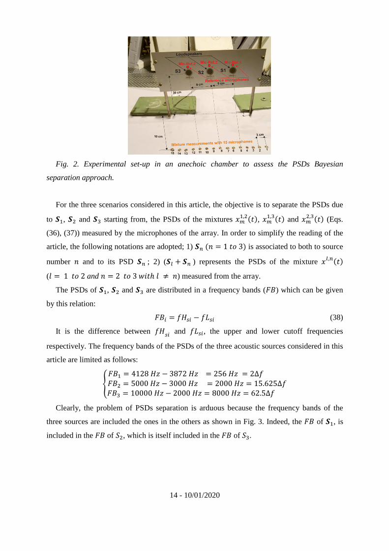
In the framework of this study, an experiment has been carried out in an anechoic chamber

(Fig.2) to assess the ability of the Bayesian approach to separate successfully the PSDs of the

acoustic sources that may be involved in practical situations encountered in the

characterization of aircraft noise.

More precisely, we are concerned to get a solution to a major problem of interest. Starting

from � the PSDs of the observations composed of a tonal source (i.e. ��), a narrowband

source (i.e. �j) occurring in propulsion devices of aircrafts, and an unwanted broadband noise

(i.e. �´) We want to truly separate out the PSDs of ��, �j and �´. These latter are three

loudspeakers ��, �j, and �´ radiating a sine wave at 4 kHz, an acoustic wave in the frequency

range [3 kHz, 5 kHz] and another on in the interval [2 kHz, 10 kHz] respectively. The

acoustic measurements are performed with a linear array composed of fifteen equally-spaced

microphones. Moreover, three reference microphones called e5<1,e5<2 and e5<3 are also

installed near the output of the loudspeaker. The acoustic waves ��(�), �j(�) and �´(�) emitted respectively by ��, �j, and �´ are individually measured with both the array and

reference microphones. According to the previous discussions on the noise generated by

propulsion devices, we only consider the three scenarios, when the pairs of loudspeakers (��, �j), (��, �´) and (�j, �´) are active. In the present situation, we are in a reverberation-free

environment with propagation delays so that the mixing model (Eq. (2)) of the three scenarios

can be simplified: %L,'(�) = *%,L(�)�LF� − 2%,LG + *%,'(�)�'F� − 2%,'G + 5%(�); " = 1,2, … ,� (36)

where

ºE, D = 1, 2»ℎ5D^�*D3^j*�5*½�¾¿5E, D = 1, 3»ℎ5D^�*D3^´*�5*½�¾¿5E, D = 2, 3»ℎ5D^j*D3^´*�5*½�¾¿5 (37)

2%,L and 2%,'are the propagation delays between microphone " and sources E and D

respectively, *%,L and *%,' are the mixing coefficients including attenuation factors (due to

propagation effects) between microphone " and sources E and D respectively.

14 - 10/01/2020

Fig. 2. Experimental set-up in an anechoic chamber to assess the PSDs Bayesian

separation approach.

For the three scenarios considered in this article, the objective is to separate the PSDs due

to ��, �j and �´ starting from, the PSDs of the mixtures %�,j���, %�,´��� and %j,´��� (Eqs.

(36), (37)) measured by the microphones of the array. In order to simplify the reading of the

article, the following notations are adopted; 1) �'�D 1�g3� is associated to both to source

number D and to its PSD �'; 2) (�L 4 �') represents the PSDs of the mixture L,'��� (E 1�g2 and D 2�g3»¾�¼E À D) measured from the array.

The PSDs of ��, �j and �´ are distributed in a frequency bands (ÁÂ) which can be given

by this relation: ÁÂS <�US 1 <;US (38)

It is the difference between <�US and <;US, the upper and lower cutoff frequencies

respectively. The frequency bands of the PSDs of the three acoustic sources considered in this

article are limited as follows:

¹ÁÂ� 4128�� 1 3872�� 256�� 2∆<ÁÂj 5000�� 1 3000�� 2000�� 15.625∆<Á´ 10000�� 1 2000�� 8000�� 62.5∆< Clearly, the problem of PSDs separation is arduous because the frequency bands of the

three sources are included the ones in the others as shown in Fig. 3. Indeed, the Á of ��, is

included in the ÁÂ of j, which is itself included in the ÁÂ of ´.

15 - 10/01/2020

Fig. 3. Sketch showing the width of the frequency bands of the PSDs of the acoustic waves

radiated by the three loudspeakers.

The PSDs separation based on a Bayesian approach takes on its full meaning since prior

information on the primary source PSDs can be exploited to help the their separation from the

PSDs of the observations. Indeed, as it is indicated in Fig. 4, we have �� and �j which radiate

in frequency ranges much narrower than �´, and �� in a much narrower frequency range than �j. This naturally leads to use a sparsity prior in the frequency domain for �� when it is

mixed with �j or �´ and for �j when it is mixed with �´ to solve the separation problem.

Fig. 4. From top to bottom, comparison of the width of the frequency bands of the PSDs when

the sources (��, �´), (�j, �´) and (��, �j) are active to justify the use of sparsity prior.

It is pointed out that in the experiment, the microphones of the array are in the far-field of

the acoustic sources ��, �j and �´, in the frequency range [1 kHz, 15 kHz] where the three

following criteria are satisfied [40]: e ≫ Ædj/�2Ç� (39) e ≫ d (40) e ≫ Ç/�2Æ� (41)

16 - 10/01/2020

where e = 0.316" is the shortest distance from the sources to the measurement positions,

λ the wavelength of radiated sound and d = 0.03", is the loudspeaker diameter.

Indeed, the second criterion ((Eq. (40)) is always satisfied since; e = 0.316 ≫ d = 0.03".

Moreover, the higher frequency f = 15 kHz of the emission range, leads to Ç%S' = 0.022".

Thus, the two criteria (Eqs. (39) - (41)) give:

e = 0.316 ≫sȸ

jÉ= (3.14)

. ´¸

(j)( . jj)= 0.064" ; e = 0.316 ≫

É

js=

. jj

(j)(´.�Ê)= 0.0035";

In the same way, the lower frequency f = 1 kHz of the emission range, leads to Ç%RË =

0.34", thus we the two criteria (Eqs. (39) - (41)) that give:

e = 0.316 ≫sȸ

jÉ= (3.14)

. ´¸

(j.)( .´Ê)= 0.0041" ; e = 0.316 ≫

É

js=

.´Ê

(j)(´.�Ê)= 0.054".

This simple verification allows to confirm that the microphones of the array are in the farfield

of S�, Sj and S´ where the sound pressure decreases inversely with the distance.

In contrast, the reference microphones used to build the simulated data are in the nearfield,

adjacent to the hydrodynamic field (a region very close to the vibrating surface of the

sources). In this area, measurements of the acoustic pressure amplitude give an inaccurate

indication of the sound power radiated by the sources [40] due of the presence of interferences

between contributing waves from various parts of the sources. Thus, it is difficult to forecast

the sound pressure levels in this area because it does not necessarily decrease monotonically

at the rate of 6 dB for each doubling of the distance from the sources.

5 TESTS WITH ARTIFICIAL MIXTURES

Before proceeding with the PSDs separation starting from, the PSDs of the measured

mixtures, a preliminary step was performed with artificial mixtures of the real source signals.

Thus, the signals at the output of the reference microphones R5<1, e5<2 and e5<3 were

filtered in frequency bands [3.8 kHz, 4.2 kHz], [1 kHz, 8 kHz] and [0.3 kHz, 14 kHz]

respectively. The results of the filtering constitute the primary source signals��(�), �j(�) and

�´(�). These latter were numerically mixed pairwise according to the model described by (Eq.

(36)).

As explained at the conclusion of the previous section, measurements performed in near-

field with the reference microphones give an inaccurate indication of the sound power levels

17 - 10/01/2020

radiated by ��, �j, and �´. Therefore, the magnitudes of the PSDs of the signals at the output

of the microphones in farfield cannot be deduced from these measurements. Thus, we have

adapted the mixing coefficients in Eq.(36) in order to obtain the same magnitudes that those

computed with real mixtures measured with the farfield microphones during the experiment

presented in Section 5.

5.1 Analysis of artificial mixtures

The upper plots in Fig.5 show the time series of �� the tonal source, �j the narrowband

source and �Ì the broadband source measured with the microphones R5<1, e5<2 and e5<3.

The plots in the center present the histogram of ^� where two regions are dominant for which

the amplitude of �� is either the lowest or the highest. The histograms of �j and �´ exhibit a

bell shape (center and right graphs) corresponding to a Gaussian distribution. Scatters

displayed in the lower plots depict joint distributions of the primary sources. It appears that �Í

and �j (left graph), �� and �´ (center graph) are independent with uniform distribution on a

parallelogram. However, the scatter plots for �  and �´ show, this time, two independent

Gaussian distributions which are rotationally symmetrical (right graph).

Fig. 5. Primary source signals ��, �j and �´ measured with filtering of e5<1, e5<2, and e5<3 shown in Fig.2 (top) - Histograms of ��, �j and �´ (center) - Joint distributions of (��, �j), (��, �´) and (�j, �´) (bottom).

18 - 10/01/2020

The upper graphs in Fig.6 present the time series of the artificial mixtures %�,j(�), %�,´(�) and %

j,´(�) (Eq. (36)) obtained when the sources (�� 4 �j), (�� 4 �´) and (�j 4 �´) are

respectively active, and measured by the "#$ (" = 1g�2) microphone of the array. It

appears that the histograms of the mixtures tend to be bell-shaped (center graphs in Fig. 6).

The scatter plots in the lower graphs show that the mixtures %�,j��� and %j,´��� are no longer

independent from each other. However, it is not evident to give the same conclusion for the

mixture %�,´���, which looks like an independent Gaussian distribution.

Figure 6. Artificial mixtures ��� 4 �j�, ��� 4 �´� and ��j 4 �´� of the primary source

signals in the upper plots in Fig.5 (top) - Histogram of the mixtures (center) - Joint

distributions of the mixtures (bottom).

The upper graphs in Fig.7 exhibit the PSDs of the primary source signals shown in Fig.5

(upper graphs). In the center, it is superimposed from left to right, the PSDs of (��, �j), (��,

�´) and (�j, �´), while the lower graphs display the PSDs of the mixtures %�,j���, %�,´��� and %j,´���. These latter will be used as input data of the separation methods proposed in the

article to obtain the unmixed PSDs (��, �j), (��, �´) and (�j, �´).

19 - 10/01/2020

Fig.7. PSDs of primary source signals shown in the upper plots of Fig.5 (top) - Superposition

of source signal PSDs (��, �j), (��, �´) and (�j, �´) (center) – PSDs of the primary source

signals mixed artificially (»ℎ5�5�L + �' = ]^dg<F�L(�) + �'(�)G»¾�ℎ(E, D) =(1,2�;�1,3�;�2,3�� (bottom).

6 PRIORS FOR THE SOURCE PSDs AND THE MIXING MATRIX –

LIKELIHOOD DESCRIPTION

The approach considered in this study is based on the Joint Maximum A Posterior (JMAP)

to solve the separation problem of the PSDs of the sources S. The JMAP estimator (Eq.(29))

requires to define the priors ¢���, ¢��� and the likelihood ¢��|�, �� composing the posterior

probability ¢��, �|�� (Eq. (26)). The forward model for � (Eq. 18)) is used to describe the

observations considered in Section 8.

6.1 PSDs priors

We have different possible priors for the PSDs of the sources ��, �j and �´, depending on

many design choices, and each combination of these choices, giving a different algorithm. We

assess the Bayesian separation capability of the PSDs for two kinds of priors described in the

next sections.

20 - 10/01/2020

6.1.1 Gaussian priors for the PSDs of �

We first consider that there is no specific knowledge of the acoustic PSDs. This leads to

adopting a Gaussian distribution as prior law, with zero-mean, and of dispersion law �X.j (D=1

to 3) for��, �j and �´, so that:

^'~£F�'�Ï, �X.j \G ∝ 5 ¢ ¦− 12�U.j ‖�'‖jj§ (42)

where ‖. ‖jj is the Frobenius norm.

6.1.2 Sparsity prior and Gaussian priors for the PSDs of �

In this second case one assumes that some knowledge on the acoustic PSDs of � is

available when �� is mixed with �j or �´ and when �j is mixed with �´. It is shown in Fig. 4

that the PSDs of �� or �j can be defined, sparse (i.e. has only few nonzero elements in the

frequency domain) compared to the PSDs of �´ and the PSD of �j sparse compared to the

PSD of �´. The sparsity of the PSD can be translated via Laplace density: �'~ℒ(�'|Ñ') ∝ 5 ¢¯−Ñ'‖�'‖� °, D = 1g�2 (43)

where ‖. ‖� is the ;� norm.

Moreover, when a sparsity prior is affected to the PSD of ��, a Gaussian one is considered

for the PSDs of �j and �´ because it is again assumed that we have no specific knowledge on

the PSDs of �j and �´. For the same reason, when a sparsity prior is affected to the PSD of �j

a Gaussian one is attributed to the PSD of �´. 6.2 Mixing matrix prior

The elements of the mixing matrix � reflect the coupling between the acoustic sources and

the observations achieved by the microphones. Nevertheless, the time signatures of the

primary sources ��, �j and �´ needed to obtain their PSDs, cannot be accurately measured

by using the reference microphones R5<1, e5<2 and e5<3 for the reasons explained at the

end of Section 4. Therefore, the coefficients of the mixing matrix are not available. It is why;

we consider here, that the mixing process may be modelled generically because it is not well

understood. In order to represent our state of ignorance, a Gaussian distribution of zero-mean

with a diagonal covariance matrix �­j\ is applied to the mixing matrix. Thus:

�~£(�|Ï, �­j\) ∝ 5 ¢ ¦− 12�­j ‖�‖jj§ (44)

21 - 10/01/2020

6.3 Likelihood

The PSD of the noise associated to the experimental measurements can reasonably be

represented as a centered Gaussian process:

�~£(�|Ï, ��j\) ∝ 5 ¢ ¦− 12��j ‖�‖jj§ (45)

The choice of the noise covariance indicates that each component of � in Eq. (18) is

contaminated by independent identically distributed random noise. The likelihood can be

therefore written in the following form:

¢(�|�, �, ¬�) ∝ 5 ¢ ¦− 12��j ‖� − ��‖jj§ (46)

7 JMAP SOLUTIONS FOR THE DATA ANALYSIS

We have defined in Section 3.2 the principle of the optimization method for obtaining

generic JMAP solutions �® and �® for the mixing matrix � and � the PSDs of the primary

sources. In the following, we examine the possible solutions for the mixing cases defined by

Eqs.(36) and (37), by using Eqs.(42), (43), (44) and (45) for the PSDs priors, the matrix prior

and the likelihood respectively.

7.1 JMAP - Gaussian priors for the PSDs of � In this first situation, we consider that the PSDs of the three acoustic sources ��, �j and �´ have Gaussian priors defined by Eq. (42). By taking into account the prior for A (Eq. (44))

and the likelihood (Eq.(45), the JMAP estimator becomes (Eq.(33)):

³(�, �) = 12��j ‖� − �L�L − �'�'‖jj + 12�­j ‖�‖jj + 12�XÒj ‖�L‖jj + 12�X.j ‖�'‖jj (47)

As it is indicated in Section 3.2, the solutions of the cost function ³(�, �) is based on an

alternate optimization with respect to � and then to �. During the iterative process (Eq. (35)),

closed-form solutions are used to compute estimates of � (when �L and �' are assumed to be

known, E and D defined in Eq. (37)) and of �L (when � and �' are assumed to be known) and

of �' (when � and �L are assumed to be known). This leads to a three step Alternating Least

Squares (ALS) algorithm [39]:

?@A@B lÓ = t Ó�F Ó Ó� + Ç­\Gq� ÓL = FlÓL�lÓL + ÇXÒ\Gq�(lÓL�t − lÓ'�lÓL Ó')Ó' = FlÓ'�lÓ' + ÇX.\Gq�(lÓ'�t − lÓL�lÓ' ÓL) (48)

22 - 10/01/2020

where:

?@@@A@@@B Ç­ = ��j�­jÇXÒ = ��j�XÒj ÇX. = ��j�X.j

(49)

7.2 JMAP SPARSE - Sparsity prior for the PSD of �Í and Gaussian for the PSDs of �  and �Ì In the second scenario corresponding to the case where �� is mixed with �j or �´

(Eq.(36)), one considers that the PSD of �� is sparse and has a Laplace prior Eq. (43). It is

also assumed that the PSDs of �j and �´ have Gaussian priors (Eq. (34)). By taking into

account the prior for � (Eq.(44)) and the likelihood (Eq.(45)), the JMAP estimator (Eq.(33))

becomes:

³(�, �) = 12��j ‖� − �L�L − ����‖jj + 12�­j ‖�‖jj + 12�XÒj ‖�L‖jj + Ñ�‖��‖� (50)

where the subscript E = 2 or E = 3 are used when �j or �´ is respectively active.

Thus, according to Eq. (35), the estimates of � and � can be obtained using a three step

algorithm ALS:

?@A@B lÓ = argmin� {‖� − �L�L − ����‖jj + Ç­‖�‖jj} ÓL = argminXÒ ¯‖� − �L�L − ����‖jj + ÇXÒ‖�L‖jj°Ó� = *�hminX� ¯‖� − �L�L − ����‖jj + Ç�‖��‖� °

(51)

where:

?@@A@@B Ç­ = ��j�­jÇXÒ = ��j�XÒj Ç� = Ñ���j

(52)

Closed-form solutions are applied to compute estimates of � (when �j or �´ is assumed to

be known) and �j or �´ (when � and �� are assumed to be known) during the iterative

process:

23 - 10/01/2020

¹ �® = t Ó�F Ó Ó� + Ç­\Gq��®L = FlÓL�lÓL + ÇXÒ\Gq�(lÓL�t − lÓ'�lÓL Ó') (53)

In contrast, the non-differentiability of the penalty function Ç�‖��‖� in the objective

function ³(�Í) = ‖� − �L�L − ����‖jj + Ç�‖��‖� deriving from Eq.(50) so that there is no

closed-form solution for ³(�Í) that can be used in the update rule for obtaining �®� in the ALS

algorithm (Eq. (53)). Therefore, we necessitate to employ an optimization scheme for this

step. The Ô� norm regularized least squares LASSO (Least Absolute Shrinkage and Selection

Operator) [41] that seeks the minimizer of ³(�Í) is chosen in the optimization process

because it provides the best performance in the sense of the sparsity/measurement trade-off.

7.3 JMAP SPARSE - Sparsity prior for the PSD of �  and Gaussian for the PSD of �Ì This last example is quite similar to the scenario examined in Section 7.2, but here a

sparsity prior is applied for the PSD of �j and a Gaussian for the PSD of �´ (the subscripts 1

and E are replaced with 2 and 3 respectively in Eqs. (49), (50) and (51)). Again, the non-

differentiability of the penalty function Çj‖�j‖� in the objective function ³(� ) =‖� − �j�j − �´�´‖jj + Çj‖�j‖� , prevents to have closed-form solutions for ³(� ) that can

be used in the update rule for the solution �®j. This step is again done with regularized least

squares LASSO.

7.4 Initialization of ALS algorithm

The ALS solutions given by Eqs. (47) and (50) depends on the parameters λ© and λª in

the Eqs.(48) and (51) initialized to positive, arbitrary values for the three scenarios presented

in Section 8. However, the determination of those parameters is not easy, in this work we

tried to obtain optimal the values of λ© (in a range λ©Ö×Ø ≤ λ© ≤ λ©ÖÙÚ) and λª (in a range λªÖ×Ø ≤ λ© ≤ λªÖÙÚ) by fixing the optimality criterion to be a good separation of the PSDs of

the acoustic sources.

As in all iterative algorithms, the initialization step is needed in the ALS algorithm (Eqs

(48) and (51)). A good initialization can improve the speed and accuracy of the algorithm, as

it can produce faster convergence an improved minimum. We have achieved satisfactory

results by initializing Û with ones values, λ© and λª in the following way:

1. Scenario # 1 – Gaussian priors for the PSDs of �

24 - 10/01/2020

The PSDs of Ü�, Üj and Ü´ are initialized with the signal PSDs of the signals at

the outputs of the three first microphones of the array and the parameter values of λ© and λª obtained during the ALS iterative processing are:

• λ© = 100 is kept with the same value for the two other scenarios;

• λª� =λª¸ = λªÝ = 0.0001 when the PSDs have Gaussian priors of equal

variances;

• ÇXÒ = 0.1 and ÇX. = 0.4 (the subscripts E = 1; D = 2g�3, Eq. (37)) when the

PSDs have Gaussian priors of non equal variances.

2. Scenario # 2 – Sparsity prior for�ℎ5]^dg<�� and Gaussian priors for the

PSDs of �j and �´ The PSD of Ü� is initialized with ones everywhere, the PSDs of Üj and Ü´

directly by using the PSDs of the signals at the outputs of the two first

microphones of the array and the parameter values λª obtained during the ALS

iterative process are:

• ÇXÒ = 0.1 and ÇX. = 0.35 (the subscripts E = 1; D = 2g�3). 3. Scenario # 3 – Sparsity prior for the PSD of �  and Gaussian one for the PSD of �Ì

The PSD of Üj is initialized with ones everywhere and the PSD of Ü´ directly by

using the PSD of the signal at the output of the first microphone of the array and

the parameter values λª obtained during the ALS iterative process are:

• ÇXÒ = 0.1 and ÇX. = 0.35 (the subscripts E = 2; D = 3). 8 SEPARATION RESULTS

The PSDs Bayesian separation algorithms presented in Section 7 are applied here on the

data recorded during the experiment described in Section 4. In the first part, we examine the

separation results of the PSDs of the primary source signals obtained starting from � (Eq.

(18)), the vector of the PSDs of the observations, mixed artificially (see Section 5). In the

second part, the results are analyzed when the vector � is computed with the mixtures

measured with the array of microphones (see Section 4). For both kinds of trials:

- the mixing matrix (Eq. (44)) and the likelihood (Eq. (45)) have Gaussian priors;

25 - 10/01/2020

- all PSDs priors are first considered Gaussian, then sparse and Gaussian, when the

observations are mixed artificially, but the priors are only sparse and Gaussian when the

observations are measured.

8.1 Separation results obtained from PSDs of observations mixed artificially

8.1.1 Results based on Gaussian priors for the PSDs of�

8.1.1.1 Gaussian priors of same variance

In this scenario, one considers that the PSDs of the primary sources have all a Gaussian

prior of same the variance (�X�j = �Xj = �XÝj in Eq. (47)). As specified in Sec. 7.4, we have for Ç­ = 100 and ÇX� =ÇX¸ =ÇXÝ = 0.0001.

The PSDs of the observations mixed artificially pairwise shown in the lower graphs in

Fig.7, are unmixed in the right part in Fig.8 based on Eqs.(47), (48) and (49). We observe that �®� (upper and center plots) and �®j (bottom plot) are very noisy. By comparing the solutions

(�®�, �®j) and (�®�, �®´) to the original source PSDs (��, �j) and (��, �´) (left plots in Fig.8),

we realize that it is non obvious to conclude that �®� characterizes the PSD of a tone source at

4kHz. In contrast, �®j and �®´ are very similar than the original PSDs �j and �´. Finally,

separation results for the PSDs of the mixture (�j + �´) show that �®´ reproduces the spectral

shape of the PSD of �´, but the same conclusion cannot be applied for �®j which does not

clearly exhibit that the PSD of �j is spread in the frequency range [2 kHz, 5 kHz].

8.1.1.2 Gaussian priors of not equal variances

This time the variances of the Gaussian priors considered for the PSDs of the primary

sources are not equal (¾. 5.�XÒj ≠ �X.j in Eq. (49)). As defined in Sec. 7.4, ÇXÒ = 0.1 and ÇX. = 0.4 (the subscripts E, D are defined in Eq. (37) and ÇXÒ and ÇX. in Eq. (49)). The

separation results of the PSDs based on Eqs.(47), (48) and (49) are presented in Fig. 9 (right

plots). The results seem better compared to the those shown in Fig.8 (right plots), obtained

when the variances of the Gaussian priors were considered equal. It clearly appears that the

background noise has decreased, so that the DSP �®� of tone source at 4 kHz appears more

clearly both when �� is mixed with �j or �´. In contrast, the separation of the PSD of the

mixture (�j +�´) is again, not totally well achieved. Indeed, it is not obvious to conclude that �®j characterizes of a narrow band in the frequency range [3kHz, 5kHz] source comparing to �®´ which exhibits a broadband source.

26 - 10/01/2020

Fig.8. Separation results when the observations are mixed artificially – Left plots: PSDs (��, �j), (��, �´) and (�j, �´) of the primary sources ��, �j and �´ – Center plots PSDs

(�L + �') of the mixtures �L,'(�) in Eq. (36) (E = 1�g2; D 2�g3 with E À D)

measured with the 1st microphone of the array. Right plots: Unmixed PSDs (��, �j), (��, �´)

and (�j, �´) by using Gaussian priors of equal variances for the PSDs of ��, �j and �´.

27 - 10/01/2020

Fig.9. Separation results when the observations are mixed artificially – Left plots: PSDs (��, �j), (��, �´) and (�j, �´) of the primary sources ��, �j and �´ – Center plots PSDs

(�L + �') of the mixtures �L,'(�) in Eq. (36) (E = 1�g2 and D 2�g3»¾�¼E À D)

measured with the 1st microphone of the array – Right plots: Unmixed PSDs (��, �j), (��, �´)

and (�j, �´) using Gaussian priors of non-equal variances for the PSDs of ��, �j and �´.

8.1.2 Results with sparsity and Gaussian priors for the PSDs of S

In this Section, we are again interested to separate the PSDs of the primary source signals

which are mixed in the PSDs of the observations shown in the lower plots in Fig.7. A sparsity

prior is affected at the PSD of �� and a Gaussian one at the PSD of �j or �´. This time, the

separation is based on Eqs. (50), (51) and (52). As defined in Section 7.4, we have: Ç­ 100

, ÇXÒ 0.1 and ÇX. 0.35 (the subscripts E 1, D 2g�3). The separation of the PSDs of

the mixtures (�� +�j) and (�� +�´) is presented in the right part in Fig. 10. The interest of

sparsity prior, clearly appears compared to the results obtained with Gaussian priors plotted in

the right part in Figs. 8 and 9. Indeed, �®� shows only a peak at 4 kHz for the tonal source.

The characteristics (i.e. shape and frequency support) of the narrowband and broadband

sources are again well found with �®j and �®´ respectively.

Fig.10. Separation results when the observations are mixed artificially – Left plots: PSDs (��, �j) and (��, �´) of the primary sources��, �j and �´ – Center plots PSDs (�L 4 �') of the

mixtures �L,'��� in Eq. (36) (E 1and D 2g�3) measured with the 1st microphone of the

array – Right plots: Unmixed PSDs (��, �j) and (��, �´) using a Laplace prior for the PSD

of �� and a Gaussian priors for the PSDs of �j and �´.

28 - 10/01/2020

The separation of the PSDs of the mixture (�j +�´) presented in the right part in Fig. 11

is obtained for Ç­ = 100 , ÇXÒ 0.1 and ÇX. 0.35 (the subscripts E 2, D 3). A

sparsity prior is affected at the PSD of �j and a Gaussian one at the PSD of �´. Again, the

interest of sparsity prior appears clearly. Indeed, �j and �´ are well separated with �®j and �®´.

It was not really the case with the separation results shown in Figs.8 and 9 where Gaussian

prior was affected at the PSDs of �j and �´.

Fig.11. Separation results when the observations are mixed artificially – Left plots: PSDs (�j,

�´) of the primary sources �j and �´– Center plots PSDs (�L 4 �j) of the mixtures ��,j��� (Eq.(36)) measured with the 1st microphone of the array – Right plots: Unmixed PSDs (�j, �´) using a Laplace prior for the PSD of �j and a Gaussian prior for the PSD of �´.

8.1.3 Evaluation of the results

In order to evaluate Bayesian algorithms, applied to the observations computed with

artificial mixtures, we use the signal-to-distortion ratio (SDR) defined in [30], expressed in

decibels based on Eq. (8), as follows:

^de�3Â� 10Egh10 ∑ ∑ ��D�C��2�D1C∑ ∑ F�®D�C� 1 �D�C�G2�D1C (54)

where �' and �®' are the true and separated PSDs referring to the D#$ source respectively,

and the index C stands for the frequency index. �' (D 1,… ,�). The PSDs of the true

signals are obtained in a similar manner described at the end of Section 2.3, but in Eq. (19),

m%ℓ is substituted with �'ℓ to give:

�' 2D�∆�& ��mDℓ�  ,D 1,… , �'¡ℓ(� (55)

In each case in Table 1, the best results are achieved when Laplace and Gaussian priors are

affected to the PSDs, compared to the cases where only Gaussian priors are used.

It also appears that sparsity plays a role in the quality of the separation measured with SDR.

Indeed, SRD is maximum for the separation of the PSDs (�� +�´), then weakly decreases

29 - 10/01/2020

for the separation of the PSDs of (�� +�j) and is minimum for the separation of the PSDs of

(�j +�´).

Finally, one notices that the Gaussian priors with the same variances give higher SRDs than

when Gaussian priors with non equal variances are used.

Mixtures

�S + �r (¾ = 1; Þ = 2) �S + �r (¾ = 1; Þ = 3) �S + �r(¾ = 2; Þ = 3)

Source priors

Gaussian for �S and �r with �Xßj = �Xàj SDR = -4.40725 SDR = -2.16497 SDR = -0.926623

Gaussian for �S and �r with �Xßj ≠ �Xàj SDR = -7.48531 SDR = -8.58410 SDR = -0.273513

Laplace for �Sand

Gaussian for �r SDR = 10.8997 SDR = 12.5466 SDR = 1.90496

Table 1. Source separation performance measured with SDR

It is important to be able to measure how the PSDs are sparse or dense, one versus the

other to explain the results obtained with sparsity priors. This can be done by using a

sparseness measure based on the ℓ norm [42], that can reliably quantify the sparseness of the

PSD �S of the ¾#$ source, compared to the length of the frequency band ÁÂr (Eq.38)) of the

PSD �r of the Þ#$ source. Indeed, consider the PSD of the ¾#$ source computed for discrete

frequencies <L (E = 0, 1, … , � − 1): �¾ = [^¾(<0), ^¾(<1), … , ^¾(<�−1)] ≠ 0 (56)

Then, define the function:

<( S(<L)) = ¹1<g� S(<L) ≠ 00<g� S(<L) = 0

(57)

The norm ℓ of S is:

‖�¾‖ = & <(^¾(<E))�−1E=0

(58)

Basically, the ℓ norm of the vector �S is equal to the number of its non-zero components.

For �S ≠ 0, we have always: 0 ≤ ‖�S‖ ≤ � (59)

The most obvious sparness measure based on the ℓ norm is defined as:

á (�S) = �� − 1 (1 − ‖�S‖ � ) (60)

30 - 10/01/2020

We see that closer the measure á (�S) is to 1, the sparser is the �S. On the contrary, the

closer the measure is to 0, the denser or less sparse is the �S. One can deduce the ℓ norm of the PSDs ��, �j and �´ by basing on the Eqs. (57) and (58)

and by using the frequency bands of the PSDs of the three acoustic sources presented after Eq.

(38), thus:

¹‖��‖ = 2‖�j‖ = 15.625‖�´‖ = 62.5 (61)

Table 2 shows the comparison of the sparseness of the PSD �S compared to the length of the

frequency band ÁÂr (Eq.38)) of the PSD �r obtained with Eq. (60) but where� is substituted

with �Sr = âYà∆> (the index ¾ stands for the PSD of ¾#$ source whose we want to compare the

sparsity versus the wideness of the frequency band of the PSD of the source of index Þ). As it

was foreseeable, the measure of the sparseness á0ÁÂ3(�1) is greater á0ÁÂ2(�1) which itself

greater than á0ÁÂ3(�2), respectively obtained for the PSDs of the mixtures (�� +�´), (�� +�j)

and (�j +�´).

Laplace prior for the PSD of �Sand Gaussian one for the PSD of �r �S + �r (¾ = 1; Þ = 2) �S + �r (¾ = 1; Þ = 3) �S + �r(¾ = 2; Þ = 3)

��j = ÁÂj∆< = 15.625 �13 = ÁÂ3∆< = 62.5 �23 = ÁÂ3∆< = 62.5

á âY¸(��) = ��j��j − 1 (1 − ‖��‖ ��j ) á âYÝ(��) = �13�13 − 1 (1 − ‖��‖ �13 ) á âYÝ(�j) = �23�23 − 1 (1 − ‖�j‖ �23 ) á âY¸(��) = 0.933333 á âYÝ(��) = 0.983607 á âYÝ(�j) = 0.754098

Table 2. Measure of the sparseness of the PSD of the ¾#$ source compared to the frequency

band ÁÂr of the PSD of the Þ#$ source.

The results depicted in Table 2 tend to show that the mean SDR presented in Table 1,

decreases in a similar manner that the measure of the sparseness á (�S). 8.2 Experimental results

The Bayesian PSDs separation method previously employed in Section 7 on PSDs of the

observations artificially mixed is applied now to the PSDs of the mixtures (�� +�j), (��

+�´) and (�j+�´) measured with the microphones of the array during the experiment

described in Section 4 (Fig. 2). The reference signals e5<1, e5<2, and e5<3 due to the

31 - 10/01/2020

loudspeakers ��, �j and �´ respectively (upper plots in Fig.12) are not filtered compared to

the cases studied with the artificial mixtures (upper plots in Fig.5). The result, is that the

histogram (center plots in Fig.12) of �� characterize a Gaussian distribution and not a sine

wave as it was previously presented in the medium of Fig. 5. As anticipated, the histograms

for �j and �´ characterize Gaussian distributions. The scatter plots of the joint distributions

displayed in the lower part in Fig.12, are similar to those of independent Gaussian sources, for

(��, �j), (��, �´) and (�j, �´).

Fig.12. Real data – Source signals of ��, �j and �´ measured without filtering of e5<1, e5<2, and e5<3 shown in Fig.2 (top); Histograms of the primary sources (center); Joint

distributions of the primary sources (bottom).

The time series of the mixtures of (�� + �j), (�� + �´) and (�j + �´) measured with the

microphones 1 and 2 of the linear array are presented in the upper graphs in Fig.13. The

corresponding histograms of the mixtures measured with microphone 1, show Gaussian

distributions (center graphs). Like for the tests carried out with artificial mixtures (Fig.6

bottom), it appears that the scatter plots in the lower graphs in Fig. 13 show that the mixtures

(�� + �j), (�j + �´) are no longer independent from each other. In contrast, the mixture (��

+ �´) looks like independent Gaussian distribution.

32 - 10/01/2020

Figure 13. Real mixtures (�� + �j), (�� + �´) and (�j + �´) of the primary source signals

shown in the upper plots in Fig.12 (top) – Histogram of mixtures (center), Joint distributions

of mixtures (bottom).

The upper plots in Fig.14 exhibit the PSDs of the reference source signals e5<1, e5<2, and e5<3 due to ��, radiating a sine wave at 4 kHz, �j, a narrowband wave in the frequency

range [3 kHz, 5 kHz] and �´ a broadband wave in the interval [2 kHz, 10 kHz] respectively.

It is not surprising that the PSD of the signal due to �� is more noisier than its filtered version

(upper plots in Fig.7). However, it is not the case for the PSDs of source signals measured

with e5<2 and e5<3 which are very similar than their filtered versions. The PSDs of (�� and �j), (�� and �´) and (�j and �´) measured with microphone 1 of the array are

superimposed in the center of the Fig.14, and the PSDs of mixtures (�� +�j), (�� +�´) and

(�j+�´) in the bottom graphs.

33 - 10/01/2020

Fig.14. Real mixtures - PSDs of the reference source signals shown in the upper plots in

Fig.12 (top) - PSDs (��, �j), (��, �´) of the primary sources ��, �j and �´(center) - PSDs

of the mixtures (�� +�j), (�� +�´) and (�j+�´) displayed in the upper plots in Fig.13

(bottom).

The results obtained with data mixed artificially have clearly shown the interest to use,

both sparsity and Gaussian priors, (Figs. 10 and 11) in the improvement of the separation

quality, compared to the scenarios where only Gaussian priors are used (Fig. 8 and 9). This

justifies that we limit the application of the Bayesian separation of the PSDs in the cases

where specialty and Gaussian priors are both considered. The Gaussian priors for the mixing

matrix (Eq. (44)) and the likelihood (Eq. (45)) are again preferred, for the reasons already

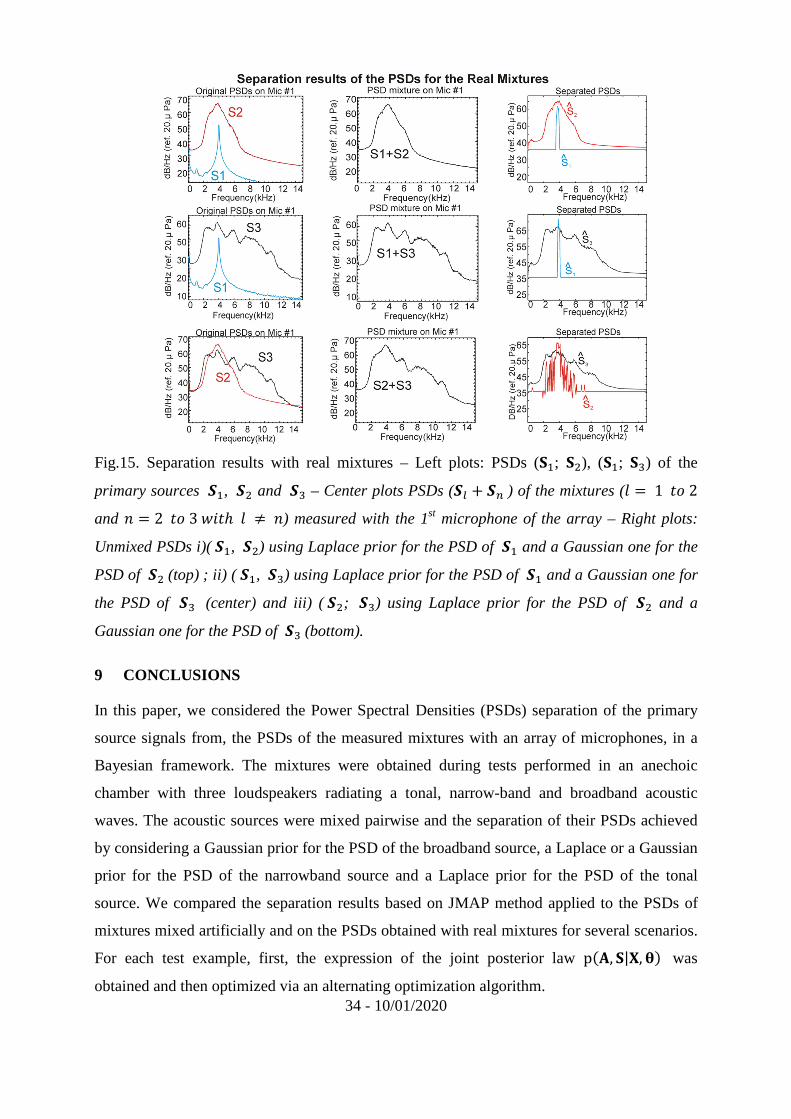
explained in Sections 6.2 and 6.3. The separation of the PSDs of the mixtures (�� +�j) and

(�� +�´) and (�j+�´) obtained with Ç­ = 800, ÇXÒ 0.09 and ÇX. 1.9 (E 1�g2 and

D 2�g3»¾�¼E À D) is presented in Fig. 15. It clearly appears that the use of sparsity

prior is quite relevant in solving the acoustic PSDs demixing problem dealt in the present

article.

34 - 10/01/2020

Fig.15. Separation results with real mixtures – Left plots: PSDs (Ü�; Üj), (Ü�; Ü´) of the

primary sources ��, �j and �´ – Center plots PSDs (�L + �') of the mixtures (E = 1�g2

and D 2�g3»¾�¼E À D) measured with the 1st microphone of the array – Right plots:

Unmixed PSDs i)(��, �j) using Laplace prior for the PSD of �� and a Gaussian one for the

PSD of �j(top) ; ii) (��, �´) using Laplace prior for the PSD of �� and a Gaussian one for

the PSD of �´ (center) and iii) (�j; �´) using Laplace prior for the PSD of �j and a

Gaussian one for the PSD of �´(bottom).

9 CONCLUSIONS

In this paper, we considered the Power Spectral Densities (PSDs) separation of the primary

source signals from, the PSDs of the measured mixtures with an array of microphones, in a

Bayesian framework. The mixtures were obtained during tests performed in an anechoic

chamber with three loudspeakers radiating a tonal, narrow-band and broadband acoustic

waves. The acoustic sources were mixed pairwise and the separation of their PSDs achieved

by considering a Gaussian prior for the PSD of the broadband source, a Laplace or a Gaussian

prior for the PSD of the narrowband source and a Laplace prior for the PSD of the tonal

source. We compared the separation results based on JMAP method applied to the PSDs of

mixtures mixed artificially and on the PSDs obtained with real mixtures for several scenarios.

For each test example, first, the expression of the joint posterior law p�Û, Ü|å, æ� was

obtained and then optimized via an alternating optimization algorithm.

35 - 10/01/2020

The main conclusions of this paper are as follows:

- first, the Bayesian approach could be used efficiently on PSDs of mixtures mixed

artificially, or obtained with measured mixtures,

- second, the measurement of the quality of the separation of the PSDs provided by the mean

Signal-to-Distortion Ratio (SDR) has clearly shown the interest to use, at the same time,

sparsity and Gaussian priors for the tests considered in the article. Indeed, this choice has

given the best results compared to the tests where only Gaussian priors are used.

- third, it is demonstrated by using a measure of the sparseness of the PSDs based on the ℓ

norm, that the quality of the separation given by SDR decreases in a similar than the degree of

sparsity of the PSDs of the acoustic sources.

10 ACKNOWLEDGMENTS

Funding for the present work was provided by Fluid Mechanics Domain and the

Aerodynamics, Aeroelasticity and Acoustics Department.

REFERENCES

[1] H. Ran and D. Mavris, « Preliminary design of a 2d supersonic inlet to maximise total

pressure recovery, » in AIAA 5th Aviation, Technology, Integration, and Operations

Conference (ATIO), Arlingto, VA, 2005.

[2] J. M. Brookfield and I. A. Waitz, « Trailing-edge blowing for reduction for reduction of

turbomachinery fan noise, » Journal of Propulsion and Power, vol. 16, no. 1, pp. 57 – 64,

January-February 2000.

[3] B. D. Mugridge, « The measurement of spinning acoustic modes generated in an axial

flow fan, » J. Sound Vib., vol. 10, no. 2, pp. 227 – 246, January-February 1969.

[4] S. Martens, « Jet noise reduction technology development at GE aircraft engines, » in

ICAS 2002 CONGRESS, 2002.

[5] Y. Li, M. Smith, X. Zhang, Measurement and control of aircraft landing gear broadband

noise, Aero. Sci. Technol. 23 (2012) 213-223.

36 - 10/01/2020

[6] Y. Tani, Y. Matsuda, A. Doi, Y. Yamashita, S. Aso, and T. Ito, « Experimental study of

the morphing flap as a low noise high lift device for aircraft wing, » in 28th International

Congress Of The Aeronautical Sciences, 2012.

[7] C. K. W. Tam, Computational Aeroacoustics A Wave Number Approach. Cambridge

University Press, 2012.

[8] I. L. Griffon, « Aircraft noise modelling and assessment in the IESTA program with focus

on engine noise, » in The 22nd International Congress on Sound and Vibration, Florence

(Italy), 2015.

[9] D. Blacodon and G. Elias, « Level estimation of extended acoustic sources using a

parametric method, » J. of Aircraft, vol. 41, no. 6, pp. 1360 – 1369, June. 2004.

[10] D. Blacodon, « Spectral estimation method for noisy data using a noise reference, »

Applied Acoustics, vol. 72, no. 1, pp. 11 – 21, January 2011.

[11] N. Chu, J. Picheral, and A. Mohammad-Djafari, « A robust super-resolution approach

with sparsity constraint in acoustic imaging, » Applied Acoustics, vol. 76, pp. 197 – 208,

February 2014.

[12] P. Comon and C. Jutten, Handbook of Blind Source Separation Independent Component

Analysis and Applications. Academic Press is an imprint of Elsevier, 2010.

[13] D.D. Lee, H.S. Seung, Learning the parts of objects by non-negative matrix factorization.

Nature 401 (6755), 788 – 791 (1999).

[14] D.D. Lee, H.S. Seung, Algorithms for non-negative matrix factorization, in Proceedings

NIPS (2000), pp. 556 – 562.

[15] P. Smaragdis and J. C. Brown, « Non-negative matrix factorization for polyphonic music

transcription, » in Proc. IEEE Workshop Applicat. Signal Process. Audio Acoust.

(WASPAA), Oct. 2003, pp. 177 – 180.

[16] N. Bertin, R. Badeau, and G. Richard, « Blind signal decompositions for automatic

transcription of polyphonic music : NMF and K-SVD on the benchmark, » in Proc. Int. Conf.

Acoust., Speech, Signal Process. (ICASSP’07), Honolulu, HI, 2007, pp. 65 – 68.

37 - 10/01/2020

[17]. A. Ozerov, C. Févotte, Multichannel nonnegative matrix factorization in convolutive

mixtures for audio source separation. IEEE Trans. Audio Speech Lang. Process. 18 (3),

550 – 563 (2010).

[18]. H. Kameoka, T. Yoshioka, M. Hamamura, J. Le Roux, K. Kashino, Statistical model of

speech signals based on composite autoregressive system with application to blind source

separation, in Proceedings of International Conference on Latent Variable Analysis and

Signal Separation (LVA/ICA) (2010), pp. 245 – 253

[19] A. Ozerov, C. Févotte, R. Blouet, J.-L. Durrieu, Multichannel nonnegative tensor

factorization with structured constraints for user-guided audio source separation, in

Proceedings of IEEE International Conference on Acoustics, Speech and Signal Processing

(ICASSP), Prague, May 2011, pp. 257 – 260.

[20] H. Sawada, R. Mukai, S. Araki, S. Makino, Convolutive blind source separation for more

than two sources in the frequency domain, in Proceeding ICASSP (2004), pp. III-885 – III-

888.

[21] H. Buchner, R. Aichner, W. Kellerman, A generalization of blind source separation

algorithms for convolutive mixtures based on second order statistics. IEEE Trans. Speech

and Audio Process. 13 (1), 120 – 134 (2005).

[22] S. Kurita, H. Saruwatari, S. Kajita, K. Takeda, F. Itakura, Evaluation of blind signal

separation method using directivity pattern under reverberant conditions, in Proceedings

ICASSP (2000), pp. 3140 – 3143.

[23] A. Hiroe, Solution of permutation problem in frequency domain ICA using multivariate

probability density functions, in Proceedings ICA (2006), pp. 601 – 608.

[24] T. Kim, H.T. Attias, S.-Y. Lee, T.-W. Lee, Blind source separation exploiting higher-

order frequency dependencies. IEEE Trans. Audio, Speech, and Lang. Process. 15 (1), 70 –

79 (2007).

[25] D. Kitamura, N. Ono, H. Sawada, H. Kameoka, H. Saruwatari, Efficient multichannel

nonnegative matrix factorization exploiting rank-1 spatial model, in Proceedings ICASSP

(2015), pp. 276 – 280.

38 - 10/01/2020

[26] D. Kitamura, N. Ono, H. Sawada, H. Kameoka, H. Saruwatari, Determined blind source

separation unifying independent vector analysis and nonnegative matrix factorization.

IEEE/ACM Trans. Audio, Speech, and Lang. Process. 24 (9), 1626 – 1641 (2016).

[27] C. Févotte and S. J. Godsill, « A Bayesian approach for blind separation of sparse

sources, » IEEE Transactions On Audio, Speech, And Language Processing, vol. 14, no. 6,

pp. 2174 – 2188, Nov. 2006.

[28] K. H Knuth, « Informed source separation : A Bayesian tutorial », Proceedings of the

13th European Signal Processing Conference (EUSIPCO 2005), Antalya, Turkey.

[29] H. Snoussi and A. Mohammad-Djafari, « A mean field approximation approach to blind

source separation with Lp priors, » in Signal Processing Conference 2005 13th European,

2005.

[30] Vincent, E., Gribonval, R., Fevotte, C. : Performance measurement in blind audio source

separation. IEEE Trans. Audio Speech Lang. Process. 14 (4), 1462 – 1469 (2006).

Source Separation Methods. Springer Press, 2007.

[31] C. Chatfield, “The Analysis of Time Series-An Introduction”, Chapman and Hall,

London, 1989, pp . 118.

[32] Julius S. Bendat, Allan G. Piersol, « Random Data: Analysis and Measurement

Procedures » Fourth Edition, John Wiley & Sons, Inc,2010, pp. 280.

[33] P. Comon, « Independent component analysis a new concept ? » Signal Processing, vol.

36, pp. 287 – 314, April 1994.

[34] A. Belouchrani, K. Abed-Meraim, J.-F. Cardoso, and E. Moulines, « A blind source

separation technique using second-order statistics, » IEEE Transactions On Signal

Processing, vol. 45, no. 2, pp. 2174 – 2188, Feb. 1997.

[35] M. S. Pedersen, J. Larsen, U. Kjems, and L. C. Parra, A Survey of Convolutive Blind

Source Separation Methods. Springer Press, 2007.

[36] Knuth K.H. 1998. Difficulties applying recent blind source separation techniques to EEG

and MEG. In : G.J. Erickson, J.T. Rychert and C.R. Smith (eds.), Maximum Entropy and

Bayesian Methods, Boise 1997, Kluwer, Dordrecht, pp. 209-222.

39 - 10/01/2020

[37] S. Winter, W. Kellermann, H. Sawada, and S. Makino, “MAP-based underdetermined

blind source separation of convolutive mixtures by hierarchical clustering and l1-norm

minimization,” EURASIP Journal on Advances in Signal Processing, Article ID 24717,

2007.

[38] A. Mohammad-Djafari, “A Bayesian approach to source separation,” in Proc. 19th

International Workshop on Bayesian Inference and Maximum Entropy Methods

(MaxEnt99), Boise, USA, Aug. 19

[39] A. Mohammad-Djafari, « Bayesian blind deconvolution of images comparing JMAP,

EM and BVA with a student-t a priori model, » in Scientific Cooperations International

Workshops on Electrical and Computer Engineering Subfields, Koç University,

Istanbul/Turkey, 2014.

[40] D.A. Bies, C.H. Hansen, Engineering Noise Control. Theory and Practice, 4th ed., Spon

Press, London, UK, 2009.

[41] R. Tibshirani, « Regression Shrinkage and Selection via the Lasso, » Journal of the Royal

Statistical Society : Series B, vol. 58, no. 1, pp. 267 – 288, 1996.

[42] Y.Huang, J. Benesty, and J.Chen, Acoustic MIMO Signal Processing. Berlin,

Germany:Springer- Verlag, 2006. 7, 10, 37.