Separate and joint inversion of dispersiveRayleigh and Love waves

Dieter Werthmuller

July 31, 2007

Bachelor Thesis

Department of Earth Sciences, ETH ZurichInstitute of Geophysics

Examiner: Jan van der KrukCo-Examiner: Sabine Latzel

Abstract

Dispersive behaviour of surface waves is observed at locations distinguishedby a layered subsurface. The dispersion characteristics depend on the thick-ness of the surface layer, the P- and S-wave velocities of the surface layerand the underlaying half space. We introduce a method to estimate theseparameters from the dispersive behaviour of Love and Rayleigh waves of aseismic measurement. This involves calculating phase velocity spectra, pick-ing dispersion curves from the spectra and inverting these dispersion curvesfor the thickness and the P- and S-wave velocity by using a combined local-and global-minimisation inversion. Separate and joint inversions from dif-ferent modes of Love and Rayleigh waves and also joint inversions of Loveand Rayleigh waves were carried out. The inversion for the thickness andthe S-wave velocities gives highly accurate results, and the joint inversion ofLove and Rayleigh waves enhanced the result. The method we present is notable to estimate the density of the subsoil.

Zusammenfassung

Oberflachenwellen zeigen in einem geschichtetem Medium ein dispersives Ver-halten. Art und Ausmass dieser Dispersion hangen unter anderem von derDicke der Oberflachenschicht und von den P- und S-Wellengeschwindigkeitender Oberflachenschicht und des darunterliegenden Halbraumes ab. Wir stelleneine Methode vor, die es erlaubt, diese Parameter aufgrund des disper-siven Verhaltens von Love- und Rayleigh-Wellen in seismischen Messungenabzuschatzen. Dies beinhaltet die Berechnung der PhasengeschwindigkeitsSpektren, Picken der Dispersionskurven in diesen Spektren sowie eine In-versionsrechnung auf Basis der gepickten Kurven, um die Dicke und dieP- und S-Wellengeschwindigkeiten zu bestimmen; invertiert wird mit Hilfeeiner kombinierten lokalen und globalen Minimisierung. Fur die verschiede-nen Moden der Dispersionskurven wurden separate wie auch kombinierteInversionen durchgefuhrt, und zusatzlich wurden auch Inversionen gerech-net, denen die Dispersionskurven von sowohl Love- als auch Rayleigh-Wellenzugrunde lagen. Die Dicke der Schicht und die S-Wellengeschwindigkeit desMediums konnten durch die Inversion gut bestimmt werden, und die kom-binierte Love-Rayleigh-Inversion vermochte das Resultat noch zu verbessern.Die vorgestellte Methode eignet sich nicht fur eine Abschatzung der Dichte.

II

Contents

1 Introduction 1

2 Theory 32.1 Seismic waves . . . . . . . . . . . . . . . . . . . . . . . . . . . . . . . . . . 32.2 Dispersive behaviour of Surface Waves . . . . . . . . . . . . . . . . . . . . 5

2.2.1 Phase velocity spectrum . . . . . . . . . . . . . . . . . . . . . . . . 62.2.2 Dispersion curves . . . . . . . . . . . . . . . . . . . . . . . . . . . . 82.2.3 Higher order modes . . . . . . . . . . . . . . . . . . . . . . . . . . 8

2.3 Forward Modelling . . . . . . . . . . . . . . . . . . . . . . . . . . . . . . . 92.4 Inversion . . . . . . . . . . . . . . . . . . . . . . . . . . . . . . . . . . . . . 10

3 Synthetic Data 123.1 Synthetic data generation . . . . . . . . . . . . . . . . . . . . . . . . . . . 123.2 Models . . . . . . . . . . . . . . . . . . . . . . . . . . . . . . . . . . . . . . 12

3.2.1 Seismograms for model 1 . . . . . . . . . . . . . . . . . . . . . . . 133.2.2 Seismograms for model 2 . . . . . . . . . . . . . . . . . . . . . . . 14

3.3 Processing . . . . . . . . . . . . . . . . . . . . . . . . . . . . . . . . . . . . 143.3.1 Phase velocity spectra for model 1 . . . . . . . . . . . . . . . . . . 143.3.2 Phase velocity spectra for model 2 . . . . . . . . . . . . . . . . . . 15

3.4 Inversion . . . . . . . . . . . . . . . . . . . . . . . . . . . . . . . . . . . . . 173.4.1 Influence of density . . . . . . . . . . . . . . . . . . . . . . . . . . . 173.4.2 Influence of P-wave velocity . . . . . . . . . . . . . . . . . . . . . . 173.4.3 Results for model 1 . . . . . . . . . . . . . . . . . . . . . . . . . . . 183.4.4 Results for model 2 . . . . . . . . . . . . . . . . . . . . . . . . . . . 21

4 Measured Data 244.1 Acquisition . . . . . . . . . . . . . . . . . . . . . . . . . . . . . . . . . . . 24

4.1.1 Three component P- and S-wave measurements . . . . . . . . . . . 244.1.2 Measurement HPP . . . . . . . . . . . . . . . . . . . . . . . . . . . 254.1.3 Measurement Degenried . . . . . . . . . . . . . . . . . . . . . . . . 26

4.2 Processing . . . . . . . . . . . . . . . . . . . . . . . . . . . . . . . . . . . . 274.2.1 Data HPP . . . . . . . . . . . . . . . . . . . . . . . . . . . . . . . . 284.2.2 Data Degenried . . . . . . . . . . . . . . . . . . . . . . . . . . . . . 28

4.3 Inversion . . . . . . . . . . . . . . . . . . . . . . . . . . . . . . . . . . . . . 304.3.1 Results for HPP . . . . . . . . . . . . . . . . . . . . . . . . . . . . 304.3.2 Results for Degenried . . . . . . . . . . . . . . . . . . . . . . . . . 32

4.4 Suggestions for additional measurements . . . . . . . . . . . . . . . . . . . 33

5 Summary and Conclusions 35

6 Acknowledgments 36

References 37

Appendix 38

III

1 Introduction

A good estimation of the geotechnical parameters of the subsurface, for example at a

building site, is very important. With this knowledge not only the risk of damage caused

by natural hazards, such as earthquakes, can be minimised, but these parameters also

contain important information about the response of a site to various inputs, such as

vibrations of machines or loading and unloading. The knowledge of these parameters

has a large influence on the construction parameters of a building, with the aim to make

it as safe and solid as possible. There are several known methods to estimate these

parameters. Some of them, such as bore hole drilling or dynamic probing, are rather

expensive and give us just local results. Furthermore, they cause a disturbance of the

subsurface.

A two- or three-dimensional image of the subsurface can be obtained by using seismic

waves in a tomographic approach. The interpretation of compressional and shear wave

traveltimes (P- and S-waves) is a very well known method (e.g. reflection and refraction

seismics, seismic tomography), whereas the surface waves, often called ground roll, are

widely regarded as noise and attempts have been made to filter them out for a long time.

Recent results [9], [11] show that surface waves contain important information about the

subsurface too, even in the small scale area of engineering interests. Several investiga-

tions are carried out using the so-called Surface Wave Method (SWM) which analyses

the dispersion curve. Usually the measurements are made using a vertical impact source,

and research focuses on the use of Rayleigh waves. Strobbia [15] and Socco [14] described

the whole procedure in detail, from acquisition over processing to inversion.

The aim of this Bachelor thesis is to improve the estimation of the S-wave velocity

by not only measuring the P-waves generated by a vertical impact source but also using

a horizontal shear source and measuring the horizontal components using three compo-

1

1 Introduction

nent geophones. From April to July 2007 existing data were processed using a combined

dispersion analysis of the normal and higher modes as well as a combined dispersion

analysis of Love and Rayleigh waves.

Chapter 2 is an introduction to the theoretical basis of this work. The investigated

methods are applied on synthetic data in Chapter 3 and on two measured datasets in

Chapter 4, and conclusions are summarised in Chapter 5.

2

2 Theory

This section gives an introduction to seismic wave propagation and to the dispersive

behaviour of surface waves. Also the principles of forward modelling and inversion are

explained.

2.1 Seismic waves

Seismic waves in an isotropic elastic medium can be split into body waves (P- and S-

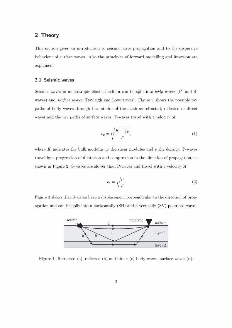
waves) and surface waves (Rayleigh and Love waves). Figure 1 shows the possible ray

paths of body waves through the interior of the earth as refracted, reflected or direct

waves and the ray paths of surface waves. P-waves travel with a velocity of

vp =

√K + 4

3µ

ρ, (1)

where K indicates the bulk modulus, µ the shear modulus and ρ the density. P-waves

travel by a progression of dilatation and compression in the direction of propagation, as

shown in Figure 2. S-waves are slower than P-waves and travel with a velocity of

vs =√

µ

ρ. (2)

Figure 3 shows that S-waves have a displacement perpendicular to the direction of prop-

agation and can be split into a horizontally (SH) and a vertically (SV) polarised wave.

c

b a

surface source receiver

layer 1

layer 2

d

Figure 1: Refracted (a), reflected (b) and direct (c) body waves; surface waves (d).

3

2 Theory

Figure 2: Body waves: P- and S-waves (from Kearey et al. [6]).

-¾ -

6

?

⊗SH

SV

Pwave propagation

Figure 3: Particle motion of SH-, SV- and P-waves.

Surface waves are slower than body waves, but they contain most of the energy of

a seismic signal or event, because the spreading of energy is in two dimensions (1/r, r

indicates the radius of spreading), whereas the spreading of energy for body waves is

in three dimensions (1/r2). When body waves hit a free surface they induce surface

waves. SH-waves generate Love waves at the surface, where SV- and P-waves generate

Rayleigh waves. The Rayleigh and Love waves are shown in Figure 4. Seismic waves are

extensively described in the literature, a good introduction is given, for example, by W.

Lowrie [10].

4

2 Theory

Figure 4: Surface waves: Rayleigh and Love waves (from Kearey et al. [6]).

2.2 Dispersive behaviour of Surface Waves

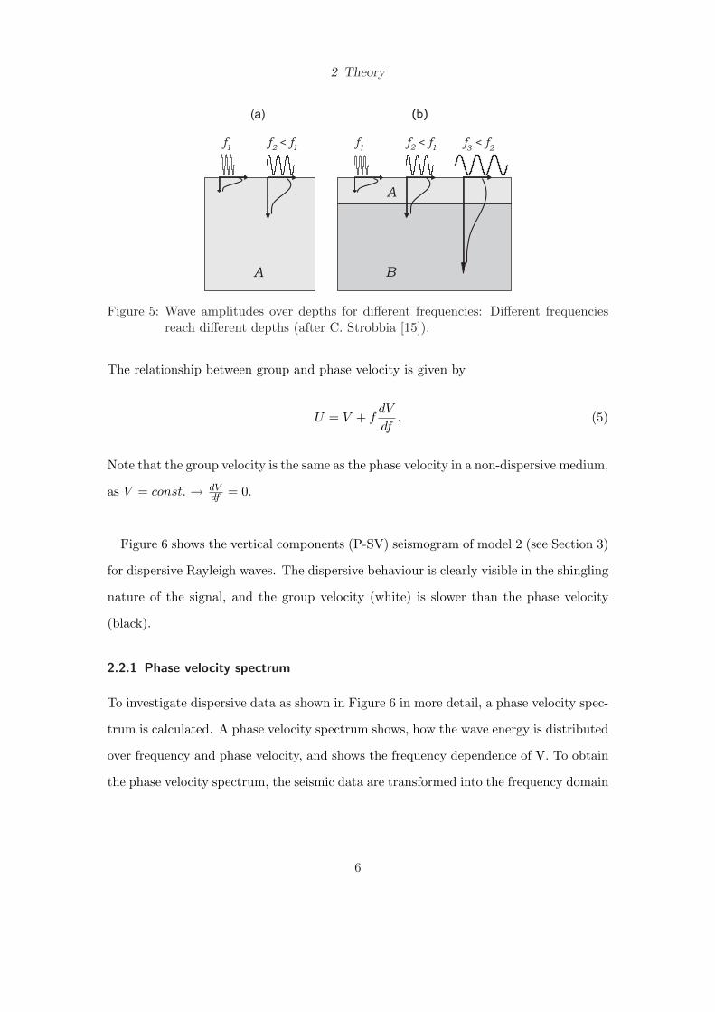
Seismic surface waves propagate along the earth’s surface, and their amplitude decreases

exponentially with depth. Surface waves reach a depth of roughly 1/3 to 1 times of their

wavelength (λ/3 to λ). Because of this, waves with lower frequencies will penetrate

deeper into the earth than those with higher frequencies (note that wavelength is equal

to velocity over frequency: λ = v/f). Figure 5 shows, that for a vertically layered

model the higher frequencies will just travel through the uppermost layer, where lower

frequencies will travel through deeper layers too. Knowing, that in most cases the

velocity increases with depth, the lower frequencies often travel with a higher speed

than the higher frequencies. The frequency dependence of phase velocity V is called

dispersion and given by

V =f

( 1λ)

. (3)

Different frequencies can travel with different velocities. The velocity with which the

energy in a wavetrain travels, is given by the group velocity U (R. E. Sheriff [13]):

U =df

d( 1λ)

. (4)

5

2 Theory

f f < f f f < f f < f1 1 1 12 2 3 2

A

A

B

(a) (b)

Figure 5: Wave amplitudes over depths for different frequencies: Different frequenciesreach different depths (after C. Strobbia [15]).

The relationship between group and phase velocity is given by

U = V + fdV

df. (5)

Note that the group velocity is the same as the phase velocity in a non-dispersive medium,

as V = const. → dVdf = 0.

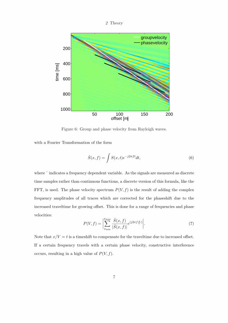
Figure 6 shows the vertical components (P-SV) seismogram of model 2 (see Section 3)

for dispersive Rayleigh waves. The dispersive behaviour is clearly visible in the shingling

nature of the signal, and the group velocity (white) is slower than the phase velocity

(black).

2.2.1 Phase velocity spectrum

To investigate dispersive data as shown in Figure 6 in more detail, a phase velocity spec-

trum is calculated. A phase velocity spectrum shows, how the wave energy is distributed

over frequency and phase velocity, and shows the frequency dependence of V. To obtain

the phase velocity spectrum, the seismic data are transformed into the frequency domain

6

2 Theory

offset [m]

time

[ms]

50 100 150 200

200

400

600

800

1000

groupvelocityphasevelocity

Figure 6: Group and phase velocity from Rayleigh waves.

with a Fourier Transformation of the form

S(x, f) =∫

S(x, t)e−j2πftdt, (6)

where ˆ indicates a frequency dependent variable. As the signals are measured as discrete

time samples rather than continuous functions, a discrete version of this formula, like the

FFT, is used. The phase velocity spectrum P (V, f) is the result of adding the complex

frequency amplitudes of all traces which are corrected for the phaseshift due to the

increased traveltime for growing offset. This is done for a range of frequencies and phase

velocities:

P (V, f) =∣∣∣∣xmax∑xmin

S(x, f)|S(x, f)|e

(j2πf xV

)

∣∣∣∣. (7)

Note that x/V = t is a timeshift to compensate for the traveltime due to increased offset.

If a certain frequency travels with a certain phase velocity, constructive interference

occurs, resulting in a high value of P (V, f).

7

2 Theory

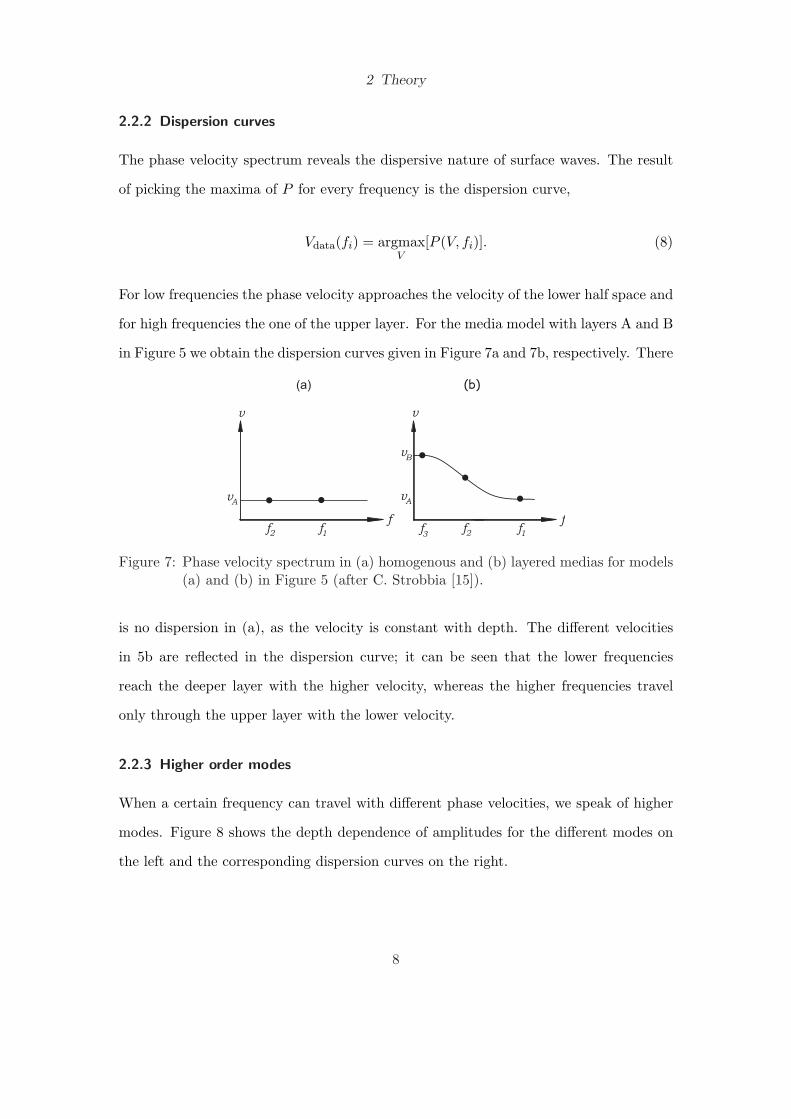
2.2.2 Dispersion curves

The phase velocity spectrum reveals the dispersive nature of surface waves. The result

of picking the maxima of P for every frequency is the dispersion curve,

Vdata(fi) = argmaxV

[P (V, fi)]. (8)

For low frequencies the phase velocity approaches the velocity of the lower half space and

for high frequencies the one of the upper layer. For the media model with layers A and B

in Figure 5 we obtain the dispersion curves given in Figure 7a and 7b, respectively. There

f1

f1

f 2f 2 f 3

ff

vA

vA

vB

v v

(a) (b)

Figure 7: Phase velocity spectrum in (a) homogenous and (b) layered medias for models(a) and (b) in Figure 5 (after C. Strobbia [15]).

is no dispersion in (a), as the velocity is constant with depth. The different velocities

in 5b are reflected in the dispersion curve; it can be seen that the lower frequencies

reach the deeper layer with the higher velocity, whereas the higher frequencies travel

only through the upper layer with the lower velocity.

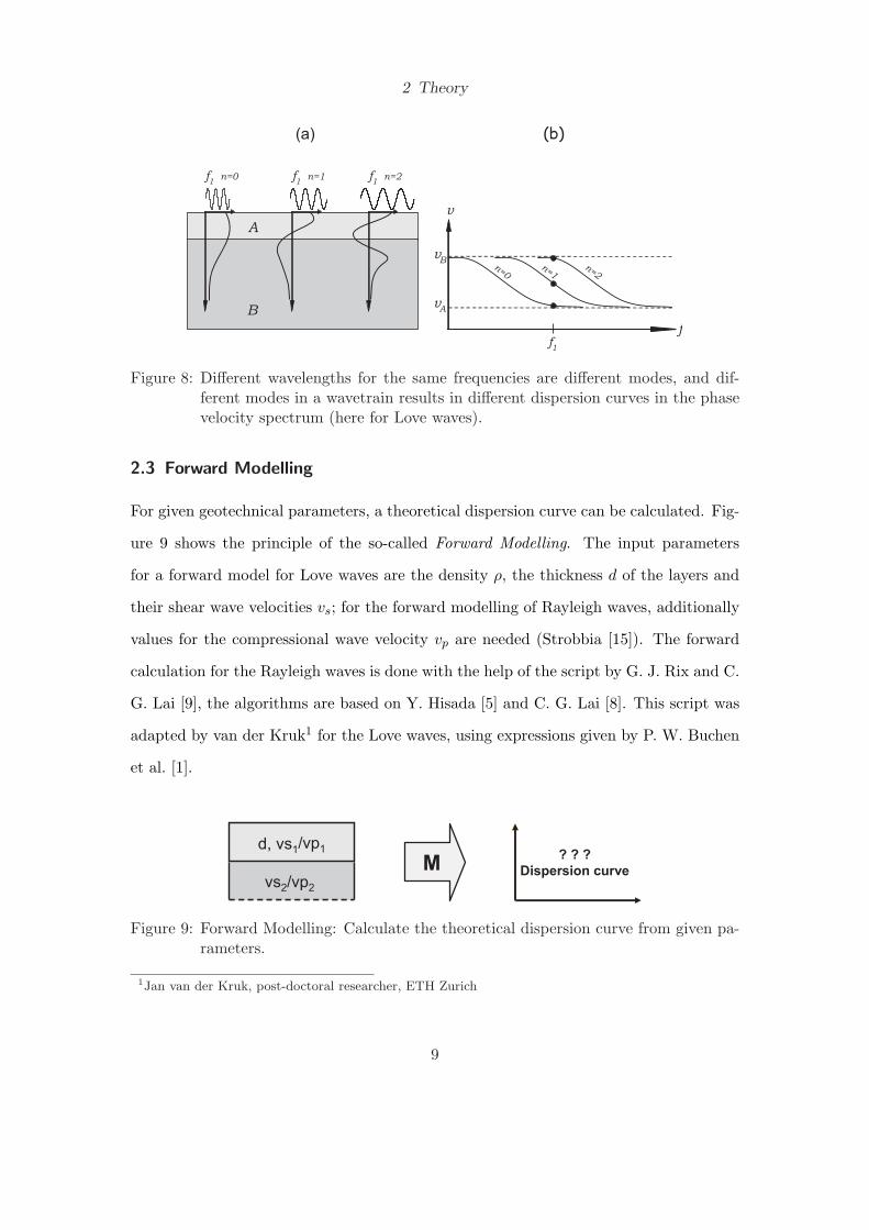
2.2.3 Higher order modes

When a certain frequency can travel with different phase velocities, we speak of higher

modes. Figure 8 shows the depth dependence of amplitudes for the different modes on

the left and the corresponding dispersion curves on the right.

8

2 Theory

f n=21

A

B

f n=01

f n=11

f

vA

vB

v

n=2n=1

n=0

f1

(a) (b)

Figure 8: Different wavelengths for the same frequencies are different modes, and dif-ferent modes in a wavetrain results in different dispersion curves in the phasevelocity spectrum (here for Love waves).

2.3 Forward Modelling

For given geotechnical parameters, a theoretical dispersion curve can be calculated. Fig-

ure 9 shows the principle of the so-called Forward Modelling. The input parameters

for a forward model for Love waves are the density ρ, the thickness d of the layers and

their shear wave velocities vs; for the forward modelling of Rayleigh waves, additionally

values for the compressional wave velocity vp are needed (Strobbia [15]). The forward

calculation for the Rayleigh waves is done with the help of the script by G. J. Rix and C.

G. Lai [9], the algorithms are based on Y. Hisada [5] and C. G. Lai [8]. This script was

adapted by van der Kruk1 for the Love waves, using expressions given by P. W. Buchen

et al. [1].

vs2/vp2

M? ? ?

Dispersion curve

d, vs1/vp1

M

Figure 9: Forward Modelling: Calculate the theoretical dispersion curve from given pa-rameters.

1Jan van der Kruk, post-doctoral researcher, ETH Zurich

9

2 Theory

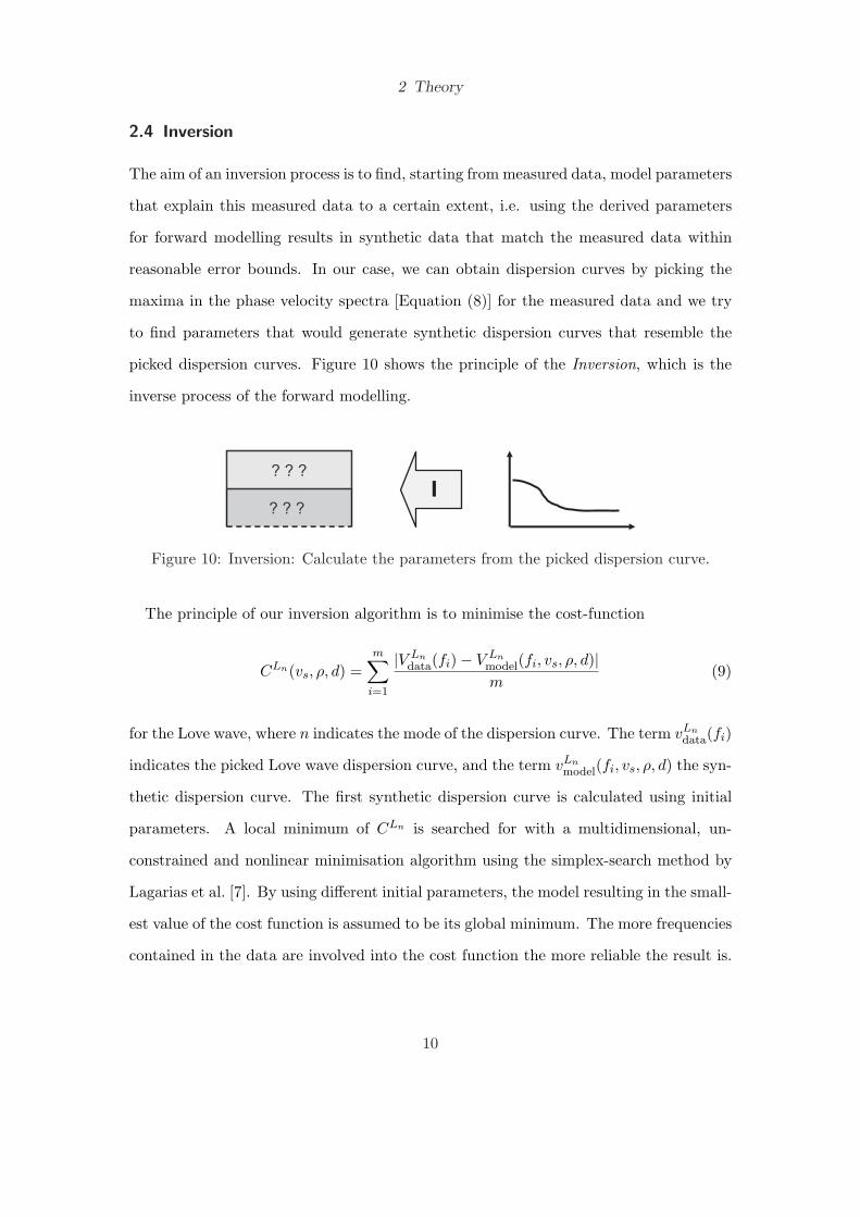
2.4 Inversion

The aim of an inversion process is to find, starting from measured data, model parameters

that explain this measured data to a certain extent, i.e. using the derived parameters

for forward modelling results in synthetic data that match the measured data within

reasonable error bounds. In our case, we can obtain dispersion curves by picking the

maxima in the phase velocity spectra [Equation (8)] for the measured data and we try

to find parameters that would generate synthetic dispersion curves that resemble the

picked dispersion curves. Figure 10 shows the principle of the Inversion, which is the

inverse process of the forward modelling.

? ? ?

? ? ?

II

Figure 10: Inversion: Calculate the parameters from the picked dispersion curve.

The principle of our inversion algorithm is to minimise the cost-function

CLn(vs, ρ, d) =m∑

i=1

|V Lndata(fi)− V Ln

model(fi, vs, ρ, d)|m

(9)

for the Love wave, where n indicates the mode of the dispersion curve. The term vLndata(fi)

indicates the picked Love wave dispersion curve, and the term vLnmodel(fi, vs, ρ, d) the syn-

thetic dispersion curve. The first synthetic dispersion curve is calculated using initial

parameters. A local minimum of CLn is searched for with a multidimensional, un-

constrained and nonlinear minimisation algorithm using the simplex-search method by

Lagarias et al. [7]. By using different initial parameters, the model resulting in the small-

est value of the cost function is assumed to be its global minimum. The more frequencies

contained in the data are involved into the cost function the more reliable the result is.

10

2 Theory

We set the minimum ratio of picked frequencies to 50%.

Similarly, the cost function for Rayleigh waves is given by

CRn(vs, vp, ρ, d) =m∑

i=1

|V Rndata(fi)− V Rn

model(fi, vs, vp, ρ, d)|m

, (10)

where n, vRndata(fi), vRn

model(fi, vs, vp, ρ, d) indicate the mode order, the picked Rayleigh

wave dispersion curve and the synthetic dispersion curve respectively.

When higher order modes are present in the data, a combined inversion can be carried

out. The cost function for combined inversion of different modes for Love and Rayleigh

waves are given by

CLa...c(vs, ρ, d) = CLa(vs, ρ, d) + · · ·+ CLc(vs, ρ, d), (11)

CRa...c(vs, vp, ρ, d) = CRa(vs, vp, ρ, d) + · · ·+ CRc(vs, vp, ρ, d), (12)

and the cost function for the joint inversion of Love an Rayleigh waves by

CLa...cRa...c(vs, vp, ρ, d) = CLa...c(vs, ρ, d) + CRa...c(vs, vp, ρ, d). (13)

11

3 Synthetic Data

A study on synthetic data was performed to get an idea of what can be expected from

measured seismic data. The reason for using synthetic data is, that the input parameters

are known and therefore it is known how the results of an inversion should look. One is

able to test all the applied algorithms, namely the forward modelling for the theoretical

dispersion curve, the picking tool and the inversion. First we describe the data generation

and the resultant seismograms. We then show the corresponding phase velocity spectra

and the inversion results.

3.1 Synthetic data generation

The synthetic seismic data were calculated by S. Latzel2 using the program flgevas

from Prof. Dr. W. Friedrich3. They are calculated for a one dimensional model and

three dimensional wave propagation for a horizontally layered earth, and modelled with

a constant visco-elastic attenuation (not frequency dependent). The data were generated

for frequencies ranging from 1Hz to 100Hz and a butterworth low-pass filter with limiting

frequency 60Hz was applied.

3.2 Models

Synthetic data were calculated for several models, the model parameters are given in

Table 1. Model 1 has parameters that are expected from the HPP measurement (see

Section 4) and model 2-7 are taken from a paper by M. Roth et al. [12]. Although we

processed all of the resulting synthetic seismograms, we only show results for models 1

and 2.

2Sabine Latzel, PhD-student, ETH Zurich3Prof. Dr. Wolfgang Friedrich, Uni Bochum

12

3 Synthetic Data

Table 1: Model parametervp1 vp2 vs1 vs2 d ρ1 ρ2 Qκ Qµ

(m/s) (m/s) (m/s) (m/s) (m) (kg/m3) (kg/m3) (-) (-)model 1 1000 2000 300 600 10 1700 2300 100 50model 2 1100 1800 330 540 5 1600 2000 100 50model 3 1100 1800 330 540 10 1600 2000 100 50model 4 1100 1800 330 540 20 1600 2000 100 50model 5 1100 1800 400 650 5 1600 2000 100 50model 6 1100 1800 450 730 5 1600 2000 100 50model 7 1100 1800 590 960 5 1600 2000 100 50

3.2.1 Seismograms for model 1

Model 1 has a upper layer thickness of d = 10m. The velocities are vp1, vp2 = 1000,

2000m/s, vs1, vs2 = 300, 600m/s, and the densities are ρ1, ρ2 = 1700, 2300kg/m3 for

the upper layer and the lower half space, respectively. Figure 11 shows the SH and

P-SV seismograms for model 1. The Love and Rayleigh waves are present in the region

enclosed by the black lines in (a) and (b) respectively, and only data lying within this

region are used for further analysis. Dispersion is obviously present, and the dispersion

behaviour of the Love waves clearly differs from that of the Rayleigh waves.

(a) SH

offset [m]

time

[ms]

50 100 150 200

200

400

600

800

1000

(b) P-SV

offset [m]

time

[ms]

50 100 150 200

200

400

600

800

1000

Figure 11: Seismograms for (a) SH and (b) P-SV waves from model 1.

13

3 Synthetic Data

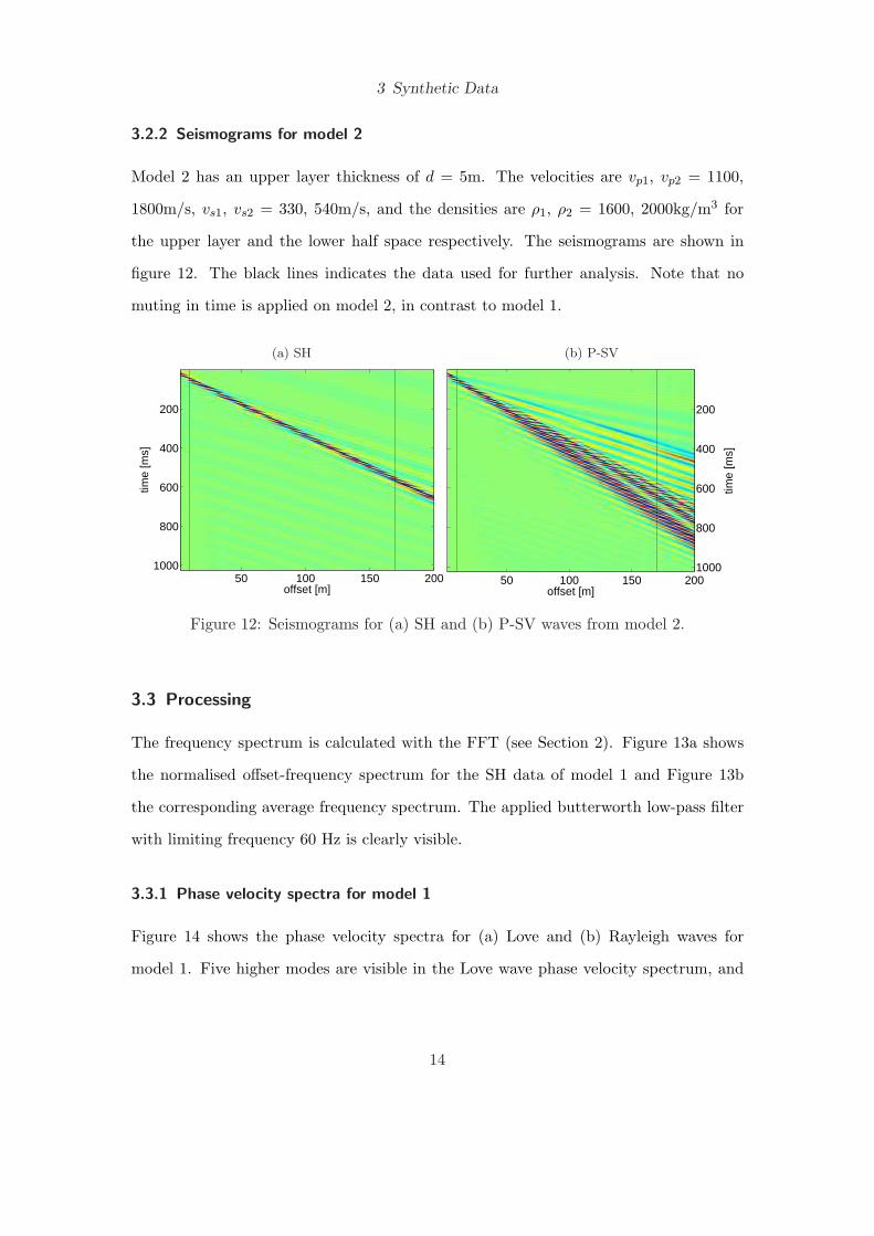
3.2.2 Seismograms for model 2

Model 2 has an upper layer thickness of d = 5m. The velocities are vp1, vp2 = 1100,

1800m/s, vs1, vs2 = 330, 540m/s, and the densities are ρ1, ρ2 = 1600, 2000kg/m3 for

the upper layer and the lower half space respectively. The seismograms are shown in

figure 12. The black lines indicates the data used for further analysis. Note that no

muting in time is applied on model 2, in contrast to model 1.

(a) SH

offset [m]

time

[ms]

50 100 150 200

200

400

600

800

1000

(b) P-SV

offset [m]

time

[ms]

50 100 150 200

200

400

600

800

1000

Figure 12: Seismograms for (a) SH and (b) P-SV waves from model 2.

3.3 Processing

The frequency spectrum is calculated with the FFT (see Section 2). Figure 13a shows

the normalised offset-frequency spectrum for the SH data of model 1 and Figure 13b

the corresponding average frequency spectrum. The applied butterworth low-pass filter

with limiting frequency 60 Hz is clearly visible.

3.3.1 Phase velocity spectra for model 1

Figure 14 shows the phase velocity spectra for (a) Love and (b) Rayleigh waves for

model 1. Five higher modes are visible in the Love wave phase velocity spectrum, and

14

3 Synthetic Data

(a) Offset-Frequency spectrum

Offset [m]

Fre

quen

cy [H

z]

50 100 150 200

0

20

40

60

80

(b) Average frequency spectrum

0 20 40 60 80 1000

0.1

0.2

0.3

0.4

0.5

0.6

0.7

0.8

Frequency [Hz]

Figure 13: (a) Offset-frequency spectrum and (b) average frequency spectrum for theSH data of model 1.

four in the Rayleigh wave phase velocity spectrum. The spectra are very noisy for low

frequencies and no dispersion curves can be picked. Note that the picked curves cover the

theoretical curves at high velocities in the Love wave case, whereas they cover just the

middle parts in the Rayleigh wave case, due to the weaker presence in the phase velocity

spectrum. The dispersion curves in the Love wave phase velocity spectrum start at the

velocity vs2 = 600m/s at low frequencies and converge to the velocity vs1 = 300m/s at

high frequencies. This feature is not present in the phase velocity spectrum for Rayleigh

waves, they show a more complicated frequency dependence.

3.3.2 Phase velocity spectra for model 2

Figure 15 shows the phase velocity spectra for model 2. In the same frequency range only

about half as many modes are present compared to model 1. Because the velocities have

similar values this must be mainly caused by the difference in thickness (note d = 5, 10m

for model 1 and 2, respectively). The phase velocity spectra are more blurred than those

for model 1, due to the fact that no muting in time is applied to cancel out the reflected

and refracted waves.

15

3 Synthetic Data

(a) Love

frequency [Hz]

Pha

se v

eloc

ity [m

/s]

20 40 60 80

300

400

500

600

700modelpicked

(b) Rayleigh

frequency [Hz]

Pha

se v

eloc

ity [m

/s]

20 40 60 80

300

400

500

600

700modelpicked

Figure 14: Normalised phase velocity spectra for (a) Love and (b) Rayleigh waves formodel 1.

(a) Love

frequency [Hz]

Pha

se v

eloc

ity [m

/s]

20 40 60 80300

350

400

450

500

550

600modelpicked

(b) Rayleigh

frequency [Hz]

Pha

se v

eloc

ity [m

/s]

20 40 60 80300

350

400

450

500

550

600modelpicked

Figure 15: Normalised phase velocity spectra for (a) Love and (b) Rayleigh waves formodel 2.

16

3 Synthetic Data

3.4 Inversion

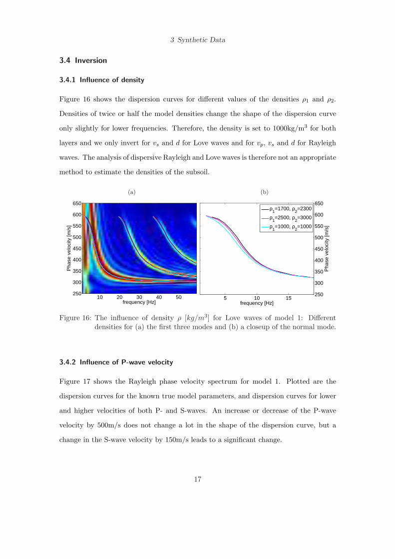
3.4.1 Influence of density

Figure 16 shows the dispersion curves for different values of the densities ρ1 and ρ2.

Densities of twice or half the model densities change the shape of the dispersion curve

only slightly for lower frequencies. Therefore, the density is set to 1000kg/m3 for both

layers and we only invert for vs and d for Love waves and for vp, vs and d for Rayleigh

waves. The analysis of dispersive Rayleigh and Love waves is therefore not an appropriate

method to estimate the densities of the subsoil.

(a)

frequency [Hz]

Pha

se v

eloc

ity [m

/s]

10 20 30 40 50250

300

350

400

450

500

550

600

650

(b)

5 10 15250

300

350

400

450

500

550

600

650

frequency [Hz]

Pha

se v

eloc

ity [m

/s]

ρ

1=1700, ρ

2=2300

ρ1=2500, ρ

2=3000

ρ1=1000, ρ

2=1000

Figure 16: The influence of density ρ [kg/m3] for Love waves of model 1: Differentdensities for (a) the first three modes and (b) a closeup of the normal mode.

3.4.2 Influence of P-wave velocity

Figure 17 shows the Rayleigh phase velocity spectrum for model 1. Plotted are the

dispersion curves for the known true model parameters, and dispersion curves for lower

and higher velocities of both P- and S-waves. An increase or decrease of the P-wave

velocity by 500m/s does not change a lot in the shape of the dispersion curve, but a

change in the S-wave velocity by 150m/s leads to a significant change.

17

3 Synthetic Data

0 5 10 15 20 25 30100

200

300

400

500

600

700

frequency [Hz]

Pha

se v

eloc

ity [m

/s]

vs1

=300, vs2

=600, vp1

=1000, vp2

=2000

vs1

=150, vs2

=450, vp1

=1000, vp2

=2000

vs1

=450, vs2

=750, vp1

=1000, vp2

=2000

vs1

=300, vs2

=600, vp1

= 500, vp2

=1500

vs1

=300, vs2

=600, vp1

=1500, vp2

=2500

Figure 17: The influence of velocity v [m/s] for Rayleigh wave dispersion curves ofmodel 1. A change in S-wave velocity has a much bigger influence than achange in P-wave velocity.

Even if P-wave velocities in the model are interchanged, the shape of the dispersion

curve changes only slightly for low frequencies. In Figure 18 the theoretical dispersion

curve for model 1 is plotted together with the theoretical dispersion curve with the same

parameters but interchanged P-wave velocities for layer and half space. Note that the

data resolution for the low frequencies is weak, as seen in Section 3.3. Hence highly

ambiguous inversion results for the P-waves are expected.

3.4.3 Results for model 1

Different modes can be identified in Figure 14 for the Love and the Rayleigh waves. They

are inverted separately and jointly for the Love and Rayleigh waves. Also combined Love

and Rayleigh dispersion curves were jointly inverted, see Table 2.

For the inversion of Love waves we used 27 different initial models with all possible

combinations of vs1 = 100, 300, 500m/s, vs2 = 400, 700, 1000m/s, and d = 3, 11.5, 20m.

For the inversion of Rayleigh waves the results of the Love wave inversions were used as

initial parameters, leading to 9 initial models with the combination of vp1 = 500, 950,

18

3 Synthetic Data

0 20 40 60 80 100250

300

350

400

450

500

550

600

frequency [Hz]

Pha

se v

eloc

ity [m

/s]

v

p1=1000, v

p2=2000

vp1

=2000, vp2

=1000

Figure 18: The influence of P-wave velocity vp [m/s] for Rayleigh wave dispersion curvesof model 1. The interchange of vp1 and vp2 has just a small influence at thelowest frequencies.

Table 2: Inversion results for separate and joint Love and Rayleigh waves of model 1.vp1 vp2 vs1 vs2 d ρ1 ρ2 C

(m/s) (m/s) (m/s) (m/s) (m) (kg/m3) (kg/m3) (m/ms)model 1 1000 2000 300 600 10 1700 2300L0 298.77 692.23 9.85 (1000) (1000) 1.21L1 299.95 644.20 9.90 (1000) (1000) 1.47L2 300.22 618.83 9.90 (1000) (1000) 1.24L01 299.23 679.38 9.93 (1000) (1000) 3.51L12 300.55 634.90 9.94 (1000) (1000) 2.99L012 299.84 652.59 9.94 (1000) (1000) 5.56R0 935.09 1558.54 300.61 615.96 9.73 (1000) (1000) 0.64R1 653.69 2394.19 303.46 745.84 10.12 (1000) (1000) 2.09R2 625.78 1582.46 303.10 757.23 10.11 (1000) (1000) 1.26R01 741.86 5231.48 302.47 734.30 10.10 (1000) (1000) 6.27R12 629.65 1685.68 303.93 833.11 10.22 (1000) (1000) 3.37R012 679.79 1449.57 303.60 799.15 10.21 (1000) (1000) 7.79L0R0 1731.29 872.83 298.93 717.91 10.18 (1000) (1000) 2.11L1R1 1470.12 1044.83 301.44 649.00 10.02 (1000) (1000) 3.34L2R2 993.68 2728.90 301.33 621.83 9.96 (1000) (1000) 2.66L01R01 1022.29 2538.42 300.20 680.46 9.99 (1000) (1000) 11.04L12R12 1092.32 2224.47 301.91 641.61 10.05 (1000) (1000) 6.78L012R012 919.78 2577.43 300.71 653.51 9.97 (1000) (1000) 10.57

19

3 Synthetic Data

1400m/s, and vp2 = 1600, 2050, 2500m/s. For the combined Love and Rayleigh wave

inversion again 27 initial models were used for all combinations of (vs1, vp1), (vs2, vp2)

and d.

The results for the separate Love and Rayleigh wave inversions are plotted in Fig-

ure 19. The inversion of Love waves is in general more stable than the inversion of

Rayleigh waves, mostly due to the bigger frequency range of the picked curve. The first

picked frequencies for the normal mode in the Love wave phase velocity spectrum are

unreliable, due to the weak resolution. The inversion results which take the normal

mode into account (L0, L01 and L012) are therefore not as good as the ones where the

normal mode is not used in the inversion. In the Rayleigh wave phase velocity spectrum

the normal mode is the one which can be picked best and reaches over the broadest

frequency range. Therefore the inversion of the normal mode gives the best result. Note

that all picked curves are fitted by one dispersion curve inversion result, note also that

the shape of the dispersion curves for Rayleigh waves is more complex than the shape

of those for the Love waves.

(a) Love

0 10 20 30 40 50 60

300

400

500

600

700

800

frequency [Hz]

Pha

se v

eloc

ity [m

/s]

modelL

0L

1L

2L

01L

12L

012picked

(b) Rayleigh

0 10 20 30 40 50 60

300

400

500

600

700

800

frequency [Hz]

Pha

se v

eloc

ity [m

/s]

modelR

0R

1R

2R

01R

12R

012picked

Figure 19: Separate (a) Love and (b) Rayleigh inversion results for model 1.

20

3 Synthetic Data

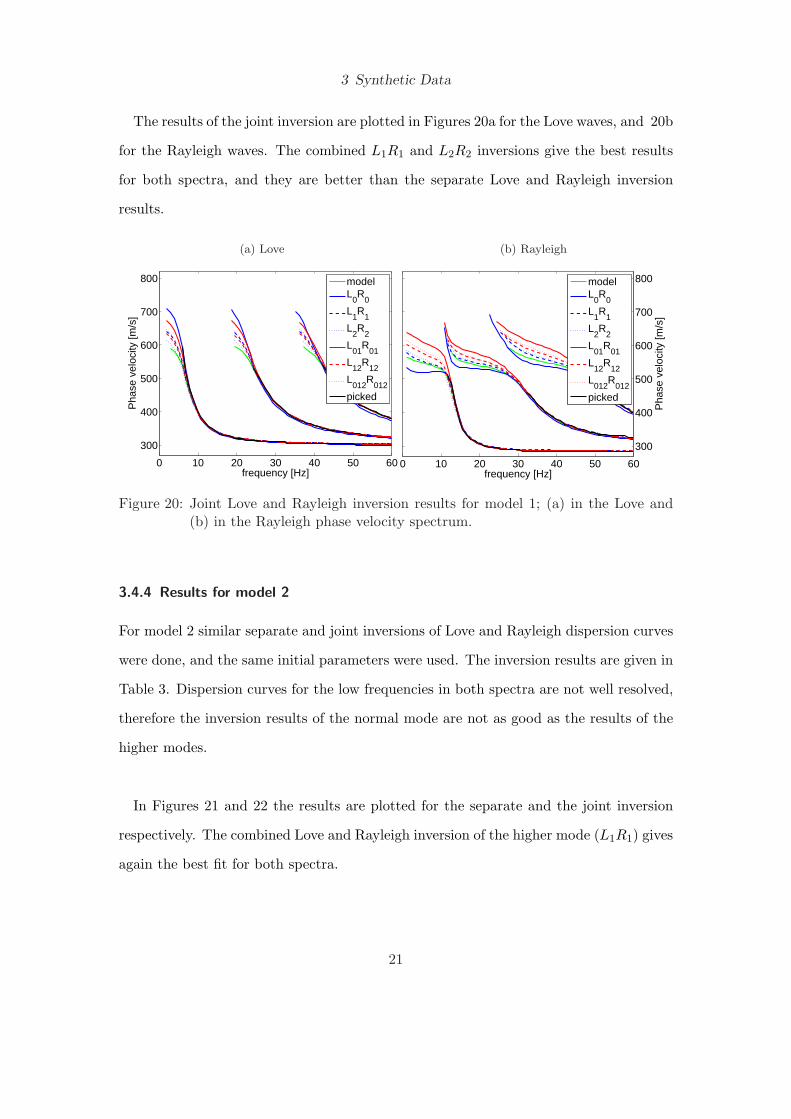
The results of the joint inversion are plotted in Figures 20a for the Love waves, and 20b

for the Rayleigh waves. The combined L1R1 and L2R2 inversions give the best results

for both spectra, and they are better than the separate Love and Rayleigh inversion

results.

(a) Love

0 10 20 30 40 50 60

300

400

500

600

700

800

frequency [Hz]

Pha

se v

eloc

ity [m

/s]

modelL

0R

0L

1R

1L

2R

2L

01R

01L

12R

12L

012R

012picked

(b) Rayleigh

0 10 20 30 40 50 60

300

400

500

600

700

800

frequency [Hz]

Pha

se v

eloc

ity [m

/s]

modelL

0R

0L

1R

1L

2R

2L

01R

01L

12R

12L

012R

012picked

Figure 20: Joint Love and Rayleigh inversion results for model 1; (a) in the Love and(b) in the Rayleigh phase velocity spectrum.

3.4.4 Results for model 2

For model 2 similar separate and joint inversions of Love and Rayleigh dispersion curves

were done, and the same initial parameters were used. The inversion results are given in

Table 3. Dispersion curves for the low frequencies in both spectra are not well resolved,

therefore the inversion results of the normal mode are not as good as the results of the

higher modes.

In Figures 21 and 22 the results are plotted for the separate and the joint inversion

respectively. The combined Love and Rayleigh inversion of the higher mode (L1R1) gives

again the best fit for both spectra.

21

3 Synthetic Data

Table 3: Inversion results for separate and joint Love and Rayleigh waves of model 2.vp1 vp2 vs1 vs2 d ρ1 ρ2 C

(m/s) (m/s) (m/s) (m/s) (m) (kg/m3) (kg/m3) (m/ms)model 2 1100 1800 330 540 5 1600 2000L0 329.82 563.82 4.88 (1000) (1000) 1.06L1 327.98 534.78 4.80 (1000) (1000) 0.37L01 330.38 558.21 4.98 (1000) (1000) 2.62R0 1225.24 752.81 329.70 596.74 5.01 (1000) (1000) 0.79R1 3287.91 788.48 326.07 561.42 4.85 (1000) (1000) 0.79R01 1922.83 748.82 328.25 576.75 4.95 (1000) (1000) 2.00L0R0 1316.52 805.91 329.55 565.23 4.89 (1000) (1000) 2.91L1R1 2049.76 3582.53 327.11 532.55 4.77 (1000) (1000) 2.25L01R01 1382.24 800.10 329.79 564.77 4.96 (1000) (1000) 6.50

(a) Love

0 20 40 60 80 100300

350

400

450

500

550

600

frequency [Hz]

Pha

se v

eloc

ity [m

/s]

modelL

0L

1L

01picked

(b) Rayleigh

0 20 40 60 80 100300

350

400

450

500

550

600

frequency [Hz]

Pha

se v

eloc

ity [m

/s]

modelR

0R

1R

01picked

Figure 21: Separate (a) Love and (b) Rayleigh inversion results for model 2.

22

3 Synthetic Data

(a) Love

0 20 40 60 80 100300

350

400

450

500

550

600

frequency [Hz]

Pha

se v

eloc

ity [m

/s]

modelL

0R

0L

1R

1L

01R

01picked

(b) Rayleigh

0 20 40 60 80 100300

350

400

450

500

550

600

frequency [Hz]

Pha

se v

eloc

ity [m

/s]

modelL

0R

0L

1R

1L

01R

01picked

Figure 22: Joint Love and Rayleigh inversion results for model 2; (a) in the Love and(b) in the Rayleigh phase velocity spectrum.

As a conclusion, we can say that the inversion of the Love wave dispersion curves

gives us more reliable results than the inversion of Rayleigh wave dispersion curves. The

additional inversion of higher modes gives a better result than the inversion of just the

normal mode, mostly due to the low resolution at low frequencies. Very good results

are gained from the jointly inverted higher modes of Love and Rayleigh waves for the

S-wave velocity and the thickness, whereas the results for the P-wave velocity are not

that good.

23

4 Measured Data

Two measured datasets were analysed with the methods described before. The measured

data are also described by D. Fah et al. [2],[3]. First, we describe the applied acquisition

method and the measurement setup. We then show the acquired seismograms, the used

data, the corresponding phase velocity spectra and the inversion results.

4.1 Acquisition

4.1.1 Three component P- and S-wave measurements

The measurements are carried out using the sledge hammer method. To generate both

P- and S-waves an iron triangle instead of an iron plate is used as a source, as illus-

trated in Figure 23. In this method each side of the triangle is hit ten times, so that

¡¡ª

@@R

¡¡

¡¡

@@

@@

¡¡ª

@@R

@@¡

¡¡@@

¡¡¡

@@

@@

@@

@@

@@

@@

B

A

A

B

?

@@

@@

@@R-A + B =

?

¡¡

¡¡

¡¡ª¾ ?

?

@@

@@

@@R-A - B =

?

¡¡

¡¡

¡¡ª¾ -¾

Figure 23: Sledge Hammer Method with an iron triangle: A hit from each side; additiongives the vertical component, subtraction gives the horizontal component.

two dataset are measured for each shot point. By stacking the ten measurements, the

noise is reduced and the quality enhanced. By adding these two datasets the horizontal

components are cancelled out, and the vertical components, the P-SV waves, are ob-

tained. By subtracting both datasets the vertical components are cancelled out, and the

horizontal components, the SH waves, are obtained. Three component geophones are

24

4 Measured Data

used, so in the end six datasets are obtained from each shot position. Especially the

vertical component for the vertical source and the horizontal component perpendicular

to the receiver plane for the horizontal source are analysed, because the P-SV and the

SH waves are present in this data.

Both measurements were made with 48 three component geophones with an eigenfre-

quency of 20Hz, arranged in a straight line with an interspace of 5m. The data were

recorded with 6 geodes, each one containing 24 channels.

4.1.2 Measurement HPP

The first measurements were carried out at Honggerberg in Zurich, close to the ETH

building called HPP. In Figure 24 the three shot points are marked, located at the

geophone-positions 1, 21 and 48. All seismograms were plotted and the phase velocity

1 21 48

0m 235m5m

Figure 24: Measurement setup for HPP: 48 receivers and 3 shot points in a straight line.

spectra calculated, and the most usable one was inverted. Figure 25 shows the seismo-

gram for the shot at receiver position 1 (HPP 1). The Love waves in the SH seismogram

and the Rayleigh waves in the P-SV seismogram are enclosed by black lines. Note that

the noisy character of the seismic data increases with growing offset. Trace 5 was deleted

in the P-SV seismogram, because the trace just contained a constant noisy signal over

the whole timeframe.

25

4 Measured Data

(a) SH

offset [m]

time

[ms]

0 50 100 150 200

200

400

600

800

1000

(b) P-SV

offset [m]

time

[ms]

0 50 100 150 200

200

400

600

800

1000

Figure 25: Seismograms for (a) SH and (b) P-SV waves from the measurement HPP 1.

4.1.3 Measurement Degenried

The second measurement was carried out at Degenried, Adlisberg in Zurich. There are

12 shot points, and in contrast to the HPP measurement the shot points are located

between two geophones as shown in Figure 26. For Degenried all the seismograms for

1.5 21.5 46.5

0m 235m5m

5.5 9.5 13.5 17.5 25.5 29.5 34.5 38.5 42.5

Figure 26: Measurement setup for Degenried: 48 receivers and 12 shot points in astraight line.

the 12 shots were plotted and the phase velocity spectra calculated, and the two clearest

ones were inverted. Figure 27 shows the seismograms for the shot position 25.5, in

positive direction (Degenried 25.5). The shot position 29.5 in positive direction can be

found in Appendix (Degenried 29.5). Note that the maximal offset in the two inverted

shots is smaller than the one in HPP 1, because the measurement setup ends after 110m

and 90m, respectively.

26

4 Measured Data

(a) SH

offset [m]

time

[ms]

0 20 40 60 80 100

200

400

600

800

1000

(b) P-SV

offset [m]

time

[ms]

0 20 40 60 80 100

200

400

600

800

1000

Figure 27: Seismograms for (a) SH and (b) P-SV waves from the measurement Degen-ried 25.5.

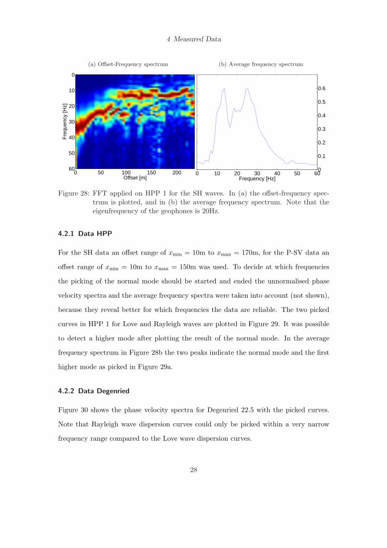
4.2 Processing

The FFT was calculated for different offsets and for different muting frames (mute in

time). Choosing too high offsets results in a noisy phase velocity spectrum, with no

visible dispersion curves, because the traces too far away from the source contain a lot

of random noise. Choosing a too small offset results in a blurry phase velocity spec-

trum, with possible overlapping of dispersion curves. Muting of noise is very important

in measured data compared to synthetic data, much better phase velocity spectra are

obtained using suitable muting. The data used for the phase velocity spectra is enclosed

by black lines in the seismogram plots. The calculated frequency spectrum for HPP 1

is plotted in Figure 28. In (a) a relationship between dominant frequency and offset is

visible: The bigger the offset, the lower the dominant frequency. In (b) the dominant

frequencies are 20Hz ± 10Hz, this is expected since geophones with an eigenfrequency

of 20Hz are used.

27

4 Measured Data

(a) Offset-Frequency spectrum

Offset [m]

Fre

quen

cy [H

z]

0 50 100 150 200

0

10

20

30

40

50

60

(b) Average frequency spectrum

0 10 20 30 40 50 600

0.1

0.2

0.3

0.4

0.5

0.6

Frequency [Hz]

Figure 28: FFT applied on HPP 1 for the SH waves. In (a) the offset-frequency spec-trum is plotted, and in (b) the average frequency spectrum. Note that theeigenfrequency of the geophones is 20Hz.

4.2.1 Data HPP

For the SH data an offset range of xmin = 10m to xmax = 170m, for the P-SV data an

offset range of xmin = 10m to xmax = 150m was used. To decide at which frequencies

the picking of the normal mode should be started and ended the unnormalised phase

velocity spectra and the average frequency spectra were taken into account (not shown),

because they reveal better for which frequencies the data are reliable. The two picked

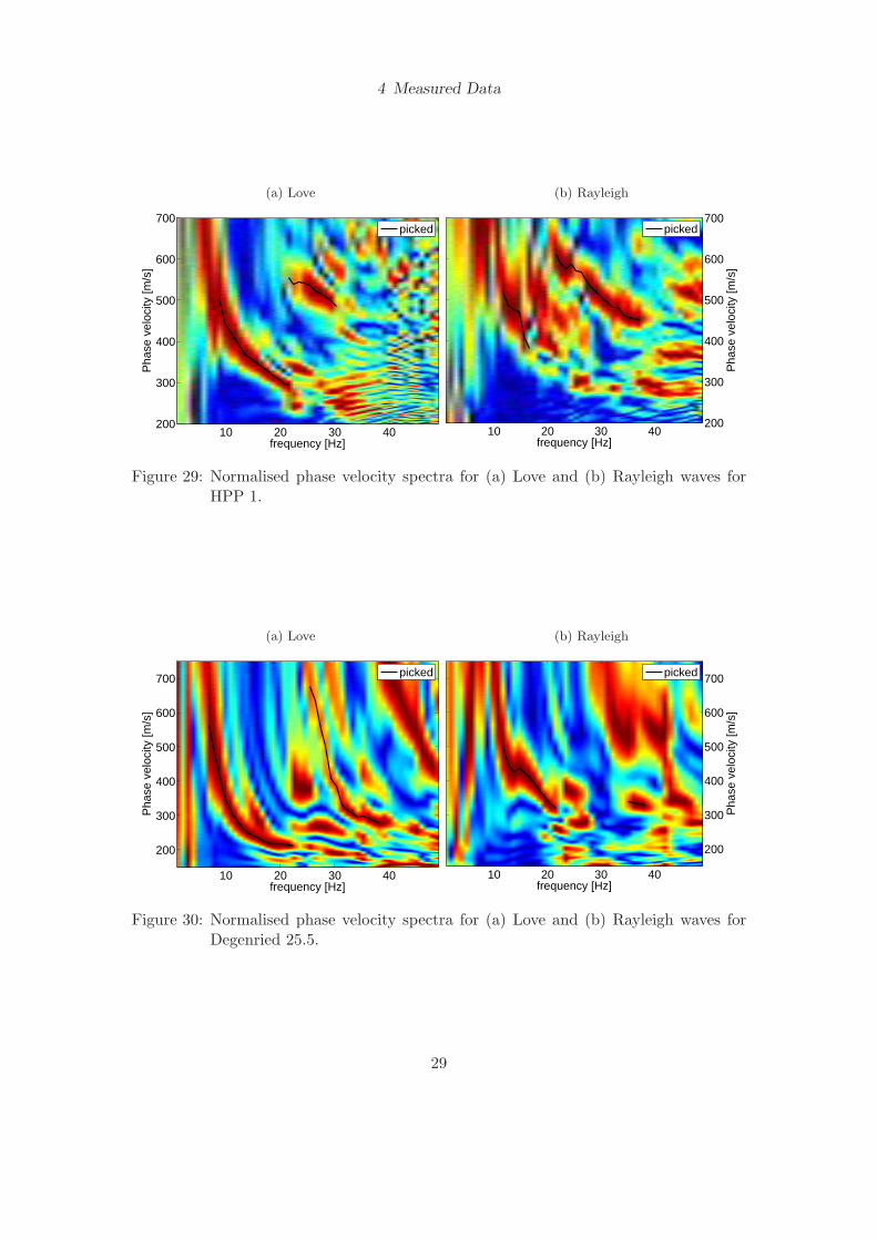
curves in HPP 1 for Love and Rayleigh waves are plotted in Figure 29. It was possible

to detect a higher mode after plotting the result of the normal mode. In the average

frequency spectrum in Figure 28b the two peaks indicate the normal mode and the first

higher mode as picked in Figure 29a.

4.2.2 Data Degenried

Figure 30 shows the phase velocity spectra for Degenried 22.5 with the picked curves.

Note that Rayleigh wave dispersion curves could only be picked within a very narrow

frequency range compared to the Love wave dispersion curves.

28

4 Measured Data

(a) Love

frequency [Hz]

Pha

se v

eloc

ity [m

/s]

10 20 30 40200

300

400

500

600

700picked

(b) Rayleigh

frequency [Hz]

Pha

se v

eloc

ity [m

/s]

10 20 30 40200

300

400

500

600

700picked

Figure 29: Normalised phase velocity spectra for (a) Love and (b) Rayleigh waves forHPP 1.

(a) Love

frequency [Hz]

Pha

se v

eloc

ity [m

/s]

10 20 30 40

200

300

400

500

600

700 picked

(b) Rayleigh

frequency [Hz]

Pha

se v

eloc

ity [m

/s]

10 20 30 40

200

300

400

500

600

700picked

Figure 30: Normalised phase velocity spectra for (a) Love and (b) Rayleigh waves forDegenried 25.5.

29

4 Measured Data

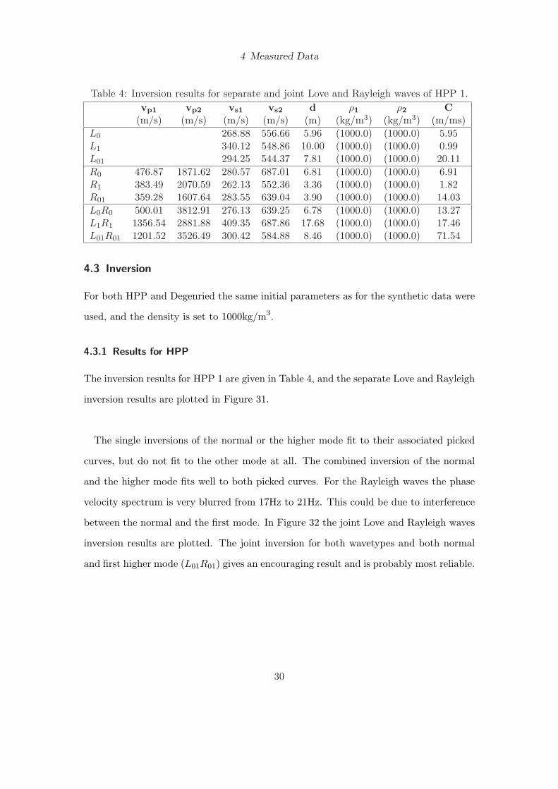
Table 4: Inversion results for separate and joint Love and Rayleigh waves of HPP 1.vp1 vp2 vs1 vs2 d ρ1 ρ2 C

(m/s) (m/s) (m/s) (m/s) (m) (kg/m3) (kg/m3) (m/ms)L0 268.88 556.66 5.96 (1000.0) (1000.0) 5.95L1 340.12 548.86 10.00 (1000.0) (1000.0) 0.99L01 294.25 544.37 7.81 (1000.0) (1000.0) 20.11R0 476.87 1871.62 280.57 687.01 6.81 (1000.0) (1000.0) 6.91R1 383.49 2070.59 262.13 552.36 3.36 (1000.0) (1000.0) 1.82R01 359.28 1607.64 283.55 639.04 3.90 (1000.0) (1000.0) 14.03L0R0 500.01 3812.91 276.13 639.25 6.78 (1000.0) (1000.0) 13.27L1R1 1356.54 2881.88 409.35 687.86 17.68 (1000.0) (1000.0) 17.46L01R01 1201.52 3526.49 300.42 584.88 8.46 (1000.0) (1000.0) 71.54

4.3 Inversion

For both HPP and Degenried the same initial parameters as for the synthetic data were

used, and the density is set to 1000kg/m3.

4.3.1 Results for HPP

The inversion results for HPP 1 are given in Table 4, and the separate Love and Rayleigh

inversion results are plotted in Figure 31.

The single inversions of the normal or the higher mode fit to their associated picked

curves, but do not fit to the other mode at all. The combined inversion of the normal

and the higher mode fits well to both picked curves. For the Rayleigh waves the phase

velocity spectrum is very blurred from 17Hz to 21Hz. This could be due to interference

between the normal and the first mode. In Figure 32 the joint Love and Rayleigh waves

inversion results are plotted. The joint inversion for both wavetypes and both normal

and first higher mode (L01R01) gives an encouraging result and is probably most reliable.

30

4 Measured Data

(a) Love

frequency [Hz]

Pha

se v

eloc

ity [m

/s]

10 20 30 40200

300

400

500

600

700L

0L

1L

01picked

(b) Rayleigh

frequency [Hz]

Pha

se v

eloc

ity [m

/s]

10 20 30 40200

300

400

500

600

700R

0R

1R

01picked

Figure 31: Separate (a) Love and (b) Rayleigh inversion results for HPP 1.

(a) Love

frequency [Hz]

Pha

se v

eloc

ity [m

/s]

10 20 30 40200

300

400

500

600

700L

0R

0L

1R

1L

01R

01picked

(b) Rayleigh

frequency [Hz]

Pha

se v

eloc

ity [m

/s]

10 20 30 40200

300

400

500

600

700L

0R

0L

1R

1L

01R

01picked

Figure 32: Joint Love and Rayleigh inversion results for HPP 1; (a) in the Love and(b) in the Rayleigh phase velocity spectrum.

31

4 Measured Data

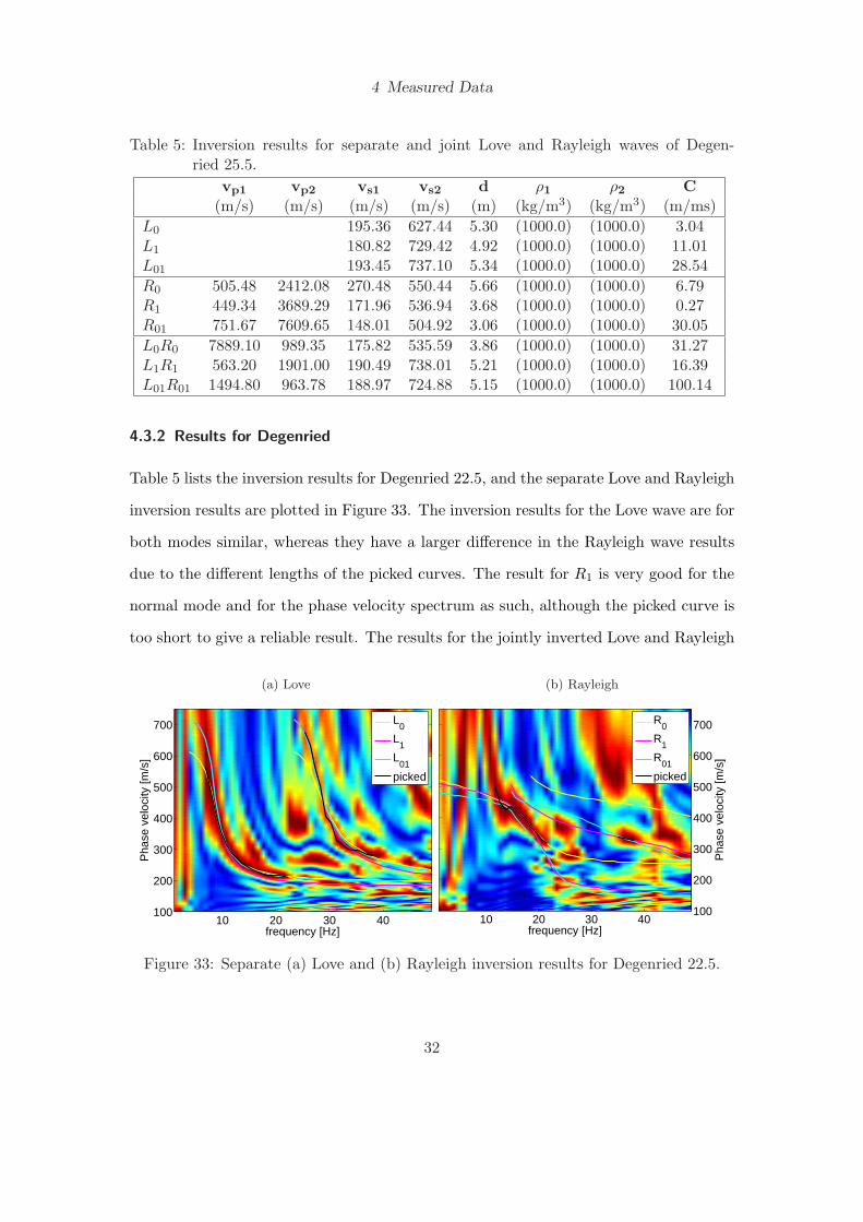
Table 5: Inversion results for separate and joint Love and Rayleigh waves of Degen-ried 25.5.

vp1 vp2 vs1 vs2 d ρ1 ρ2 C(m/s) (m/s) (m/s) (m/s) (m) (kg/m3) (kg/m3) (m/ms)

L0 195.36 627.44 5.30 (1000.0) (1000.0) 3.04L1 180.82 729.42 4.92 (1000.0) (1000.0) 11.01L01 193.45 737.10 5.34 (1000.0) (1000.0) 28.54R0 505.48 2412.08 270.48 550.44 5.66 (1000.0) (1000.0) 6.79R1 449.34 3689.29 171.96 536.94 3.68 (1000.0) (1000.0) 0.27R01 751.67 7609.65 148.01 504.92 3.06 (1000.0) (1000.0) 30.05L0R0 7889.10 989.35 175.82 535.59 3.86 (1000.0) (1000.0) 31.27L1R1 563.20 1901.00 190.49 738.01 5.21 (1000.0) (1000.0) 16.39L01R01 1494.80 963.78 188.97 724.88 5.15 (1000.0) (1000.0) 100.14

4.3.2 Results for Degenried

Table 5 lists the inversion results for Degenried 22.5, and the separate Love and Rayleigh

inversion results are plotted in Figure 33. The inversion results for the Love wave are for

both modes similar, whereas they have a larger difference in the Rayleigh wave results

due to the different lengths of the picked curves. The result for R1 is very good for the

normal mode and for the phase velocity spectrum as such, although the picked curve is

too short to give a reliable result. The results for the jointly inverted Love and Rayleigh

(a) Love

frequency [Hz]

Pha

se v

eloc

ity [m

/s]

10 20 30 40100

200

300

400

500

600

700 L0

L1

L01

picked

(b) Rayleigh

frequency [Hz]

Pha

se v

eloc

ity [m

/s]

10 20 30 40100

200

300

400

500

600

700R0

R1

R01

picked

Figure 33: Separate (a) Love and (b) Rayleigh inversion results for Degenried 22.5.

32

4 Measured Data

waves are plotted in Figure 34. The result for L0R0 is bad for the higher mode, whereas

the other two results fits well, except for the normal mode of the Rayleigh wave dispersion

curve. Because the picked curves in the Love wave phase velocity spectrum are much

longer, they influence the inversion results dominantly. Picking Love wave dispersion

curves by omitting the first three to five frequencies might enhance the inversion result.

(a) Love

frequency [Hz]

Pha

se v

eloc

ity [m

/s]

10 20 30 40

200

300

400

500

600

700 L0R

0L

1R

1L

01R

01picked

(b) Rayleigh

frequency [Hz]

Pha

se v

eloc

ity [m

/s]

10 20 30 40

200

300

400

500

600

700L0R

0L

1R

1L

01R

01picked

Figure 34: Joint Love and Rayleigh inversion results for Degenried 22.5; (a) in the Loveand (b) in the Rayleigh phase velocity spectrum.

4.4 Suggestions for additional measurements

The measurements analysed in this thesis were carried out with 48 geophones, with

a spacing of 5m and offsets from 0m to 235m. For a future acquisition with the same

equipment the suggested arrangement is a spacing of 2.5m and offsets from 10m to 225m.

This arrangement would probably result in a better resolution of the frequency spectra.

Additionally it has been shown that the signals recorded at the closest receivers do not

improve the phase velocity spectrum content, and the signal recorded at the receivers

further away are too noisy. Another point of interest are the low frequencies. The quality

of the result obtained by using the normal modes in inversion was reduced because of the

lack of information for frequencies . 5 Hz for both synthetic and measured data. Using

33

4 Measured Data

geophones with smaller eigenfrequencies over the suggested offset ranges are expected

to lead to good results.

34

5 Summary and Conclusions

We have presented a method to estimate the geotechnical parameters from the dispersive

behaviour of Rayleigh and Love waves, assuming a horizontal layer over a half space.

This method involves acquiring seismic P- and S-wave data by using the sledge hammer

method with an iron triangle and three component geophones. The data were trans-

formed from the time-offset domain to the phase velocity-frequency domain, using the

Fast Fourier Transformation. Dispersion curves for the normal and higher modes were

picked in the phase velocity spectra and used as input for the inversion. The theoretical

dispersion curves for surface waves are calculated using the density ρ, the thickness d,

and the P- and S-wave velocities vp and vs as parameters, where the density and the

P-waves have a small influence to the shape of the density curve, compared to the other

parameters. Separate and joint inversions of dispersive Rayleigh and Love waves with

several modes, using a combined local and global minimisation algorithm, yielded es-

timates of the thickness and P- and S-wave velocities of the surface layer and P- and

S-wave velocities of the underlying half space. Whereas the results of the thickness and

the S-wave velocities were highly accurate, the results for the P-wave velocities were

weak and unreliable. We suggest therefore to set the density and the P-wave velocity to

fixed values for the inversion, as done with the density in this thesis.

Our synthetic data resulted in clear phase velocity spectra, containing several higher

modes, which could be picked over a large frequency range. In the measured data the

phase velocity spectra were noisy, and picked dispersion curves are rather short. Where

the difference in the various inversion approaches is not big in the synthetic data, a joint

inversion of different modes and of the Rayleigh and Love waves enhance the results in

measured data.

The influence of the density is negligible compared to the influence of the S-wave ve-

35

locity and the layer thickness. This method is therefore not able to estimate the density

of a subsoil. The inversion of P-wave velocities is unstable and good initial values are

important. We anticipate better inversion results for the P-wave velocities, if the results

of the travel time analysis are given as initial parameters.

Although higher modes are easy to find in synthetic data they are rather hard to detect

in measured data. It turned out that the analysis of the Love waves gives better results

than the analysis of the Rayleigh waves, although P-wave measurements are easier to

carry out.

6 Acknowledgments

I want to thank Jan van der Kruk for his friendly support and invested time, which was

much more than I could have expected. I also want to thank Sabine Latzel for all the

help and advice, and the Swiss Seismological Service (Fah et al. [2],[3]) for providing the

measured data. And finally I want to thank my fellow student Kaspar Merz for making

the time at HPP O9 shorter than it actually was.

36

References

[1] P. W. Buchen and R. Ben-Hador. Free-mode surface-wave computations. Geophys-ical Journal International, 124:869–887, 1996.

[2] D. Fah, F. Matter, P. Kastli, H.-B. Havenith, H. Horstmeyer, and S. Wiemer.Standortspezifisches elastisches Antwortspektrum fur Gebaude im Bereich der ETHHonggerberg. Bericht, Schweizerischer Erdbebendienst, ETH Zurich, November2005.

[3] D. Fah and D. Roten. Stationen ZUR und SZUD: Bestimmung einesWellengeschwindigkeitsprofils. Schweizerischer Erdbebendienst, Oktober 2004.

[4] D. Gubbins. Time Series Analysis and Inverse Theory for Geophysicists. CambridgeUniversity Press, 2004.

[5] Y. Hisada. An efficient method for computing green’s functions for a layered half-space with sources and receivers at close depths. Bulletin of the Seismological Societyof America, 84(5):1456–1472, 1994.

[6] P. Kearey, M. Brooks, and I. Hill. An Introduction to Geophysical Exploration.Blackwell Publishing, third edition, 2002.

[7] J. C. Lagarias, J. A. Reeds, M. H. Wright, and P. E. Wright. Convergence propertiesof the nelder-mead simplex method in low dimensions.

[8] C. G. Lai. Simultaneous Inversion of Rayleigh Phase Velocity and Attenuation forNear-Surface Site Characterization. PhD thesis, Georgia Institute of Technology,1998.

[9] C. G. Lai and G. J. Rix. Solution of the rayleigh eigenproblem in viscoelastic media.Bulletin of the Seismological Society of America, 92(6):2297–2309, August 2002.

[10] W. Lowrie. Fundamentals of Geophysics. Cambridge University Press, 1997.

[11] G. J. Rix, C. G. Lai, and S. Foti. Simultaneous measurement of surface wavedispersion and attenuation curves. Geotechnical Testing Journal, 24(4):350–358,2001.

[12] M. Roth, K. Hollliger, and A. G. Green. Guided waves in near-surface seismicsurveys. Geophysical Research Letters, 25(7):1071–1074, April 1998.

[13] R. E. Sheriff. Encyclopedic Dictionary of Exploration Geophysics. Society of Ex-ploration Geophysicists, third edition, 1999.

[14] L.V. Socco and C. Strobbia. Surface-wave method for near-surface characterization:a tutorial. Near Surface Geophysics, pages 165–185, 2004.

[15] C. Strobbia. Surface Wave Methods. PhD thesis, Politecnico di Torino, 2002.

37

Appendix

Degenried 29.5

The seismograms for Degenried 29.5 are given in Figure 35. The used data for the

phasevelocity spectra are enclosed by the black lines. The phasevelocity spectra are

(a) SH

offset [m]

time

[ms]

0 20 40 60 80

200

400

600

800

1000

(b) P-SV

offset [m]

time

[ms]

0 20 40 60 80

200

400

600

800

1000

Figure 35: Seismograms for (a) SH and (b) P-SV waves from the measurement Degen-ried 29.5.

shown in Figure 36. The length of the picked curves is similar in both spectra. The

inversion result of the normal mode was taken into account to decide where to pick a

higher mode, as shown in Figure 37. The results for Degenried 29.5 are given in Table 6,

and they are plotted in Figures 37 and 38.

The different inversions of Love wave dispersion curves gives similar results, whereas

the different inversions of Rayleigh wave dispersion curves have big differences, due to

the very short picked curve for the higher mode. Therefore the results for the jointly

inverted Love and Rayleigh wave dispersion curves are not as good as hoped for. A good

solution might be between the solutions for L1R1 and L01R01.

38

(a) Love

frequency [Hz]

Pha

se v

eloc

ity [m

/s]

10 20 30 40 50

200

300

400

500

600

700 picked

(b) Rayleigh

frequency [Hz]

Pha

se v

eloc

ity [m

/s]

10 20 30 40 50

200

300

400

500

600

700picked

Figure 36: Normalised phasevelocity spectra for (a) Love and (b) Rayleigh waves forDegenried 29.5.

Table 6: Inversion results for separate and joint Love and Rayleigh waves of Degen-ried 29.5.

vp1 vp2 vs1 vs2 d ρ1 ρ2 C(m/s) (m/s) (m/s) (m/s) (m) (kg/m3) (kg/m3) (m/ms)

L0 201.53 640.63 5.97 (1000.0) (1000.0) 3.33L1 198.55 641.69 5.62 (1000.0) (1000.0) 5.55L01 194.69 573.97 5.40 (1000.0) (1000.0) 12.51R0 401.58 1199.87 268.16 582.51 4.26 (1000.0) (1000.0) 21.27R1 377.79 1767.86 154.56 429.48 1.36 (1000.0) (1000.0) 3.85R01 370.91 3080.41 259.80 540.37 3.66 (1000.0) (1000.0) 32.51L0R0 7672.94 7924.75 169.53 485.81 3.60 (1000.0) (1000.0) 77.63L1R1 2676.37 1805.24 253.82 830.67 7.74 (1000.0) (1000.0) 66.68L01R01 1493.49 5979.77 147.35 540.36 2.63 (1000.0) (1000.0) 136.37

39

(a) Love

frequency [Hz]

Pha

se v

eloc

ity [m

/s]

10 20 30 40 50

200

300

400

500

600

700 L0

L1

L01

picked

(b) Rayleigh

frequency [Hz]

Pha

se v

eloc

ity [m

/s]

10 20 30 40 50

200

300

400

500

600

700R0

R1

R01

picked

Figure 37: Separate (a) Love and (b) Rayleigh inversion results for Degenried 29.5.

(a) Love

frequency [Hz]

Pha

se v

eloc

ity [m

/s]

10 20 30 40 50

200

300

400

500

600

700 L0R

0L

1R

1L

01R

01picked

(b) Rayleigh

frequency [Hz]

Pha

se v

eloc

ity [m

/s]

10 20 30 40 50

200

300

400

500

600

700L0R

0L

1R

1L

01R

01picked

Figure 38: Joint Love and Rayleigh inversion results for Degenried 29.5; (a) in the Loveand (b) in the Rayleigh phasevelocity spectrum.

40