sensorless direct field oriented control of …etd.lib.metu.edu.tr/upload/12604965/index.pdf · iii...
TRANSCRIPT

SENSORLESS DIRECT FIELD ORIENTED CONTROL OF INDUCTION MACHINE BY FLUX AND SPEED ESTIMATION USING MODEL
REFERENCE ADAPTIVE SYSTEM
A THESIS SUBMITTED TO THE GRADUATE SCHOOL OF NATURAL AND APPLIED SCIENCES
OF THE MIDDLE EAST TECHNICAL UNIVERSITY
BY
GÜNAY ��M�EK
IN PARTIAL FULLFILMENT OF THE REQUIREMENTS FOR THE DEGREE OF MASTER OF SCIENCE
IN THE DEPARTMENT OF ELECTRICAL AND ELECTRONICS ENGINEERING
APRIL-2004
Approval of the Graduate School of Natural and Applied Sciences. Prof. Dr. Canan ÖZGEN Director I certify that this thesis satisfies all the requirements as a thesis for the degree of Master of Science. Prof. Dr. Mübeccel DEM�REKLER Chairman of the Department This is to certify that we have read this thesis and that in our opinion it is fully adequate, in scope and quality, as a thesis for the degree of Master of Science. Prof. Dr. Aydın ERSAK Supervisor Examining Committee Members Prof. Dr. Yıldırım ÜÇTU�
Prof. Dr. Aydın ERSAK
Prof. Dr. Muammer ERM��
Assoc. Prof. Dr.I�ık ÇADIRCI
Asst. Prof. Dr. Ahmet M. HAVA

iii
ABSTRACT
SENSORLESS DIRECT FIELD ORIENTED CONTROL OF
INDUCTION MACHINE
BY FLUX AND SPEED ESTIMATORS USING MODEL
REFERENCE ADAPTIVE SYSTEM
�im�ek, Günay
M. Sc. Department of Electrical and Electronics Engineering
Supervisor : Prof. Dr. Aydın Ersak
April, 2004
This work focuses on an observer design which will estimate flux-linkage and
speed for induction motors in its entire speed control range. The theoretical base of
the algorithm is explained in detail and its both open-loop, and closed-loop
performance is tested with experiments, measuring only stator current and voltage.
Theoretically, the field-oriented control for the induction motor drive can be
mainly categorized into two types; indirect and direct field oriented. The field to be
oriented may be rotor, stator, or airgap flux-linkage. In the indirect field-oriented
control, the slip estimation based on the measured or estimated rotor speed is
required in order to compute the synchronous speed. There is no need for the flux
estimation in such a system. For the direct field oriented case the synchronous speed
is computed with the aid of a flux estimator. In DFO, the synchronous speed is

iv
computed from the ratio of dq-axes fluxes. With the combination of a flux estimator
and an open-loop speed estimator one can observe stator-rotor fluxes, rotor-flux
angle and rotor speed. In this study, the direct (rotor) flux oriented control system
with flux and-open-loop speed estimators is described and tested in real-time with
the Evaluation Module named TMS320LF21407 and the Embedded Target software
named Vissim from Visual Solutions Company.
Keywords : Sensorless direct field oriented, flux estimation, speed estimation.
v
ÖZ
MODELE DAYANAN UYARLAMALI YÖNTEM KULLANARAK
AKI VE HIZ KEST�R�M�YLE
DUYAÇSIZ DO�RUDAN ALAN YÖNLEND�RMEL�
ENDÜKS�YON MOTOR DENET�M�
�im�ek, Günay
Yüksek Lisans, Elektrik ve Elektronik Mühendsli�i Bölümü
Tez Danı�manı : Prof. Dr. Aydın Ersak
Nisan, 2004
Bu çalı�mada endüksiyon motorunun tüm çalı�ma hızı aralıklarındaki akı ve
hızının tahmin edilemesine odakla�ılmı�tır. Sunulan yöntemin tüm kuramsal içeri�i
ayrıntılı olarak anlatılmı� ve bu yöntemin açık ve kapalı döngü ba�arımları sadece
stator akım ve gerilimlerinin ölçülmesi ile test edilmi�tir.
Teorik olarak alan yönlendirmeli endüksiyon motor denetimi iki ana grupta
incelenir; dolaylı ve do�rudan alan yönlendirmeli denetim. Yönlendirilecek alan
rotor, stator veya motor havabo�lu�u akısı olabilir. Dolaylı alan yönlendirmeli
denetimde senkron hızın hesaplanması için rotor hızının ölçülmesine veya tahmin
edilmesine gerek duyulmaktadır. Bu denetimde akı tahmin edilmesi söz konusu
de�ildir. Do�rudan alan yönlendirmeli denetimde akı tahmin yöntemi ile senkron hız
hesaplanmaktadır. Do�rudan alan yönlendirmeli denetimde dq eksenlerindeki
akıların oranından senkron hız hesaplanmaktadır. Akı tahmin ve açık-döngü hız

vi
tahmin yöntemleri yardımıyla stator ve rotor akıları, rotor akı açısı ve rotor hızı
gözlenebilmektedir. Bu çalı�mada, do�rudan alan (rotor) yönlendirmeli denetimi, akı
ve açık-döngü hız tahmin methodları kullanılarak anlatılmı� ve gerçek zamanlı
olarak da TMS320LF2407 deneme kartı ve Vissim yazılımı kullanılarak test
edilmi�tir.
Anahtar Kelimeler: Sensörsüz alan yönlendirmeli denetim, akı tahmin
methodu, hız tahmin methodu.

vii
ACKNOWLEDGMENTS
I would like to express my sincere gratitude to my supervisor Prof. Dr. Aydın
Ersak for his encouragement and guidance throughout the study. I also thank him not
only for his technical assists but for his friendship in due course of development of
the thesis.
I would also like to thank everybody at the Department of Electronic
Hardware in Aselsan for helping me with all kinds of practical problems.
Mr. Bilal Akın made significant contributions from the beginning of the study
by his technical advice, and his support always continued up to now. Mr. Eray
Özçelik helped during the experimental stage of this work. To my both dear friends I
say thank you.
The last but not least acknowledgment is to my wife, who was willing to give
up many other activities so that the study could be carried out. Her support will
always be appreciated.
viii
TABLE OF CONTENTS ABSTRACT........................................................................................................................................III ÖZ..........................................................................................................................................................V ACKNOWLEDGMENTS ................................................................................................................VII TABLE OF CONTENTS................................................................................................................VIII LIST OF FIGURES .............................................................................................................................X LIST OF SYMBOLS.........................................................................................................................XII 1 INTRODUCTION ...................................................................................................................... 1
1.1 INDUCTION MACHINE CONTROL .......................................................................................... 2 1.1.1 Field Oriented Control of Induction Machine................................................................ 3 1.1.2 Indirect Field Oriented Control ..................................................................................... 7 1.1.3 Direct Field Oriented Control........................................................................................ 8
1.2 VARIABLE SPEED CONTROL USING ADVANCED CONTROL ALGORITHMS ...........................10 1.3 OVERVIEW OF THE CHAPTERS.............................................................................................15
2 INDUCTION MACHINE MODELLING ...............................................................................16 2.1 THE INDUCTION MOTOR .....................................................................................................16 2.2 CIRCUIT MODEL OF A THREE PHASE INDUCTION MOTOR ...................................................16
2.2.1 Machine Model in Arbitrary dq0 Reference Frame ......................................................18 2.2.1.1 qd0 Voltage Equations...................................................................................................... 20 2.2.1.2 qd0 Flux Linkage Relation................................................................................................ 21 2.2.1.3 qd0 Torque Equations....................................................................................................... 22
2.2.2 qd0 Stationary and Synchronous Reference Frames.....................................................24 3 PULSE WIDTH MODULATION WITH SPACE VECTOR THEORY..............................28
3.1 INVERTERS..........................................................................................................................28 3.1.1 Voltage Source Inverter (VFI).......................................................................................29
3.2 VOLTAGE SPACE VECTORS .................................................................................................32 3.2.1 SVPWM Application to the Static Power Bridge and Implementation Using DSP Platform 34
3.3 SIMULATION AND EXPERIMENTAL RESULTS OF SVPWM...................................................39 4 FLUX AND SPEED ESTIMATION FOR SENSORLESS DIRECT FIELD ORIENTED CONTROL OF INDUCTION MACHINE .......................................................................................44
4.1 FLUX ESTIMATION ..............................................................................................................44 4.1.1 Estimation of the Flux Linkage Vector ..........................................................................45
4.1.1.1 Flux Estimation in Continuous Time ................................................................................ 45 4.1.1.2 Flux Estimation in Discrete Time ..................................................................................... 49 4.1.1.3 Flux Estimation in Discrete Time and Per-Unit................................................................ 50
4.2 SPEED ESTIMATION.............................................................................................................54 4.2.2 Speed Estimation in Discrete Time and Per-Unit..........................................................56
5 IMPLEMENTATION OF FLUX AND SPEED ESTIMATION FOR SENSORLESS DIRECT FIELD ORIENTATION ....................................................................................................60
5.1 SIMULATION RESULTS ........................................................................................................60 5.1.1 Simulation 1- For No-Load Case ..................................................................................61 5.1.2 Simulation 2-For 0.5pu Loading ...................................................................................64 5.1.3 Simulation 3-For 0.2pu and 0.3 pu Loading .................................................................67

ix
5.1.4 Simulation 4-Trapezoidal Loading................................................................................70 5.1.5 Simulation 5-Trapezoidal Speed Command ..................................................................73
5.2 EXPERIMENTAL RESULTS....................................................................................................75 5.2.1 Experimental Results-For no-load ................................................................................75 5.2.2 Experimental Results- For 0.1pu torque loading ..........................................................83
5.3 CONCLUSION OF THE SIMULATIONS AND EXPERIMENTS .....................................................86 6 THE HARDWARE & SOFTWARE........................................................................................87
6.1 THE MOTOR ........................................................................................................................87 6.2 THE MOTOR DRIVE.............................................................................................................90 6.3 THE DSP.............................................................................................................................92 6.4 INTERFACE CARD................................................................................................................93 6.5 CURRENT INTERFACE CARD ...............................................................................................95 6.6 SOFTWARE OVERVIEW........................................................................................................96
6.6.1 Base Values and PU model ...........................................................................................97 6.6.2 Fixed-Point Arithmetic ..................................................................................................98
7 CONCLUSION AND FUTURE WORK ...............................................................................100 7.1 CONCLUSION ....................................................................................................................100 7.1 FUTURE WORK .................................................................................................................100
REFERENCES..................................................................................................................................102 A APPENDIX ..............................................................................................................................106
ELECTRONIC CARDS .................................................................................................................106 B APPENDIX ..............................................................................................................................114
ACQUISITION OF THE STATOR VOLTAGES ............................................................................114 C APPENDIX ..............................................................................................................................117
HYPERSTABILITY THEORY .....................................................................................................117

x
LIST OF FIGURES FIGURE 1-1 PHASOR DIAGRAM OF THE FIELD ORIENTED DRIVE SYSTEM.................................................. 5 FIGURE 1-2 FIELD ORIENTED INDUCTION MOTOR DRIVE SYSTEM ............................................................ 6 FIGURE 1-3 INDIRECT FIELD ORIENTED DRIVE SYSTEM ........................................................................... 6 FIGURE 1-4 DIRECT FIELD ORIENTED DRIVE SYSTEM .............................................................................. 6 FIGURE 2-1 RELATIONSHIP BETWEEN ABC AND ARBITRARY DQ0 ...........................................................19 FIGURE 2-2 MODEL OF AN INDUCTION MACHINE IN THE ARBITRARY REFERENCE FRAME.......................21 FIGURE 2-3 MODEL OF AN INDUCTION MACHINE IN THE ARBITRARY REFERENCE FRAME.......................22 FIGURE 2-4 MODEL OF AN INDUCTION MACHINE IN THE STATIONARY FRAME........................................25 FIGURE 2-5 MODEL OF AN INDUCTION MACHINE IN THE STATIONARY FRAME........................................25 FIGURE 2-6 MODEL OF AN INDUCTION MACHINE IN THE SYNCHRONOUS FRAME ....................................26 FIGURE 2-7 MODEL OF AN INDUCTION MACHINE IN THE SYNCHRONOUS FRAME ....................................27 FIGURE 3-1 CIRCUIT DIAGRAM OF VFI...................................................................................................29 FIGURE 3-2 THREE PHASE INVERTER WITH SWITCHING STATES..............................................................30 FIGURE 3-3 EIGHT SWITCHING STATE TOPOLOGIES OF A VOLTAGE SOURCE INVERTER...........................31 FIGURE 3-4 FIRST SWITCHING STATE –V1..............................................................................................32 FIGURE 3-5 REPRESENTATION OF TOPOLOGY 1 IN (DS-QS) PLANE ...........................................................33 FIGURE 3-6 NON-ZERO VOLTAGE VECTORS IN (DS-QS) PLANE .................................................................33 FIGURE 3-7 REPRESENTATION OF THE ZERO VOLTAGE VECTORS IN (DS-QS) PLANE .................................34 FIGURE 3-8 VOLTAGE VECTORS .............................................................................................................36 FIGURE 3-9 PROJECTION OF THE REFERENCE VOLTAGE VECTOR ............................................................37 FIGURE 3-10 SIMULATED WAVEFORMS OF DUTY CYCLES, ( TAON, TBON,TCON ) ...........................................40 FIGURE 3-11 SECTOR NUMBERS OF VOLTAGE VECTOR ..........................................................................40 FIGURE 3-12 SVPWM OUTPUTS OF TWO PHASES...................................................................................41 FIGURE 3-13 SVPWM OUTPUTS OF TWO PHASES IN SMALL TIMESCALE ................................................42 FIGURE 3-14 LOW-PASS FILTERED FORM OF PWM1 PULSES ..................................................................42 FIGURE 3-15 LOW-PASS FILTERED FORM OF PWM1 AND PWM5 PULSES ..............................................43 FIGURE 4-1 THE WAVEFORMS OF ROTOR FLUX ANGLE IN BOTH DIRECTIONS..........................................57 FIGURE 5-1 MOTOR TORQUE AT NO-LOAD .............................................................................................61 FIGURE 5-2 MOTOR CURRENTS (ID, IQ) IN ROTATING REFERENCE FRAME AT NO-LOAD ...........................62 FIGURE 5-3 ESTIMATED ROTOR FLUX ANGLE AT NO-LOAD.....................................................................62 FIGURE 5-4 SPEED COMMAND, MOTOR ESTIMATED AND ACTUAL SPEEDS AT NO-LOAD..........................63 FIGURE 5-5 CURRENTS (IS
D AND ISQ) IN STATIONARY REFERENCE FRAME AT NO-LOAD ...........................64
FIGURE 5-6 MOTOR TORQUE AT 0.5PU.LOADING....................................................................................65 FIGURE 5-7 MOTOR CURRENTS IE
D AND IEQ IN ROTATING REFERENCE FRAME AT 0.5PU LOADING............66
FIGURE 5-8 ESTIMATED ROTOR FLUX ANGLE AT 0.5PU LOADING ...........................................................66 FIGURE 5-9 SPEED COMMAND, MOTOR ESTIMATED AND ACTUAL SPEEDS AT 0.5PU. LOADING ...............67 FIGURE 5-10 MOTOR TORQUE AT 0, 0.2 AND 0.3 PU. LOADING ...............................................................68 FIGURE 5-11 MOTOR CURRENTS IE
D AND IEQ IN ROTATING REFERENCE FRAME AT 0.2 AND 0.3 PU
LOADING.......................................................................................................................................69 FIGURE 5-12 ESTIMATED ROTOR FLUX ANGLE AT 0.2 AND 0.3PU LOADING............................................69 FIGURE 5-13 SPEED COMMAND, MOTOR ESTIMATED AND ACTUAL SPEEDS AT 0, 0.2 AND 0.3PU. LOADING
.....................................................................................................................................................70 FIGURE 5-14 MOTOR TORQUE AT TRAPEZOIDAL LOADING .....................................................................71 FIGURE 5-15 MOTOR CURRENTS (IE
D AND IEQ) IN ROTATING REFERENCE FRAME AT TRAPEZOIDAL
LOADING.......................................................................................................................................71 FIGURE 5-16 ESTIMATED ROTOR FLUX ANGLE AT TRAPEZOIDAL LOADING ............................................72 FIGURE 5-17 SPEED COMMAND, MOTOR ESTIMATED AND ACTUAL SPEEDS AT TRAPEZOIDAL LOADING .72 FIGURE 5-18 MOTOR TORQUE AT TRAPEZOIDAL SPEED COMMAND ........................................................73

xi
FIGURE 5-19 ESTIMATED ROTOR FLUX ANGLE AT TRAPEZOIDAL SPEED COMMAND ...............................74 FIGURE 5-20 SPEED COMMAND, MOTOR ESTIMATED AND ACTUAL SPEEDS ............................................75 FIGURE 5-21 CH1 ESTIMATED ROTOR FLUX ANGLE, CH2 ACTUAL ROTOR FLUX ANGLE, CH4 LINE
CURRENT AT 10HZ SUPPLY FREQUENCY .......................................................................................77 FIGURE 5-22 CH1 ESTIMATED ROTOR FLUX ANGLE, CH2 ACTUAL ROTOR FLUX ANGLE, CH4 LINE
CURRENT AT 20HZ SUPPLY FREQUENCY .......................................................................................77 FIGURE 5-23 CH1 ESTIMATED ROTOR FLUX ANGLE, CH2 ACTUAL ROTOR FLUX ANGLE, CH4 LINE
CURRENT AT 30HZ SUPPLY FREQUENCY .......................................................................................78 FIGURE 5-24 CH1 ESTIMATED ROTOR FLUX ANGLE, CH2 ACTUAL ROTOR FLUX ANGLE, CH4 LINE
CURRENT AT 40HZ SUPPLY FREQUENCY .......................................................................................79 FIGURE 5-25 STATIONARY FRAME CURRENTS (IS
D , CHANNEL 1AND ISQ , CHANNEL 2), LINE CURRENT AT 5
HZ ................................................................................................................................................80 FIGURE 5-26 STATIONARY FRAME CURRENTS (IS
D , CHANNEL 1AND ISQ , CHANNEL 2), LINE CURRENT AT
10 HZ ...........................................................................................................................................80 FIGURE 5-27 STATIONARY FRAME CURRENTS (IS
D , CHANNEL 1AND ISQ , CHANNEL 2), LINE THE CURRENT
AT 30HZ .......................................................................................................................................81 FIGURE 5-28 STATIONARY FRAME CURRENTS (IS
D , CHANNEL 1AND ISQ , CHANNEL 2), LINE CURRENT AT
40HZ ............................................................................................................................................81 FIGURE 5-29 ESTIMATED SPEED VERSUS SUPPLY FREQUENCY ...............................................................83 FIGURE 5-30 CH1 ACTUAL ROTOR FLUX ANGLE, CH2 ESTIMATED ROTOR FLUX ANGLE, CH4 LINE
CURRENT AT 10HZ SUPPLY FREQUENCY FOR 0.1 PU LOADING ......................................................84 FIGURE 5-31 CH1 ACTUAL ROTOR FLUX ANGLE, CH2 ESTIMATED ROTOR FLUX ANGLE, CH4 LINE
CURRENT AT 20HZ SUPPLY FREQUENCY FOR 0.1 PU LOADING ......................................................85 FIGURE 5-32 CH1 ACTUAL ROTOR FLUX ANGLE, CH2 ESTIMATED ROTOR FLUX ANGLE, CH4 LINE
CURRENT AT 30HZ SUPPLY FREQUENCY FOR 0.1 PU LOADING ......................................................85 FIGURE 5-33 CH1 ACTUAL ROTOR FLUX ANGLE, CH2 ESTIMATED ROTOR FLUX ANGLE, CH4 LINE
CURRENT AT 40HZ SUPPLY FREQUENCY FOR 0.1 PU LOADING ......................................................86 FIGURE 6-2 APPROXIMATE PER PHASE EQUIVALENT CIRCUIT FOR AN INDUCTION MACHINE ..................89 FIGURE 6-3 DIAGRAM OF DC MEASUREMENT .........................................................................................89 FIGURE 6-4 DC-LINK CIRCUIT ................................................................................................................91 FIGURE 6-5 INVERTER CIRCUIT ..............................................................................................................92 FIGURE 6-6 DSP INTERFACE CARD .........................................................................................................95 FIGURE 6-7 CURRENT INTERFACE CARD.................................................................................................96 FIGURE 6-8 MULTIPLICATION IN DSP ACCUMULATORS ..........................................................................99 FIGURE A-1 DSP INTERFACE CARD......................................................................................................106 FIGURE A-2 LAYOUT OF DSP INTERFACE CARD...................................................................................107 FIGURE A-3 VIEW OF DSP INTERFACE CARD ......................................................................................108 FIGURE A-4 CURRENT INTERFACE CARD..............................................................................................109 FIGURE A-5 LAYOUT OF CURRENT INTERFACE CARD ...........................................................................110 FIGURE A-6 VIEW OF CURRENT INTERFACE CARD................................................................................111 FIGURE A-7 VIEW OF DSP CARD .........................................................................................................112 FIGURE A-8 VIEW OF THE OVERALL SETUP ..........................................................................................113

xii
LIST OF SYMBOLS
SYMBOL
emd back emf d axis component
emq back emf q axis component
ieds d axis stator current in synchronous frame
ieqs q axis stator current in synchronous frame
isds d axis stator current in stationary frame
isqs q axis stator current in stationary frame
iar Phase-a rotor current
ibr Phase-b rotor current
icr Phase-c rotor current
ias Phase-a stator current
ibs Phase-b stator current
ics Phase-c stator current
Lm Magnetizing inductance
Lls Stator leakage inductance
Llr Rotor leakage inductance
Ls Stator self inductance
Lr Rotor self inductance
Rs Stator resistance
Rr Referred rotor resistance
qmd reactive power d axis component
qmq reactive power q axis component
Tem Electromechanical torque
Tr Rotor time-constant
Vas Phase-a stator voltage
Vbs Phase-b stator voltage
Vcs Phase-c stator voltage

xiii
Var Phase-a rotor voltage
Vbr Phase-b rotor voltage
Vcr Phase-c rotor voltage
Vsds d axis stator voltage in stationary frame
Vsqs q axis stator voltage in stationary frame
Veds d axis stator voltage in synchronous frame
Veqs q axis stator voltage in synchronous frame
Vdc Dc-link voltage
Xm Stator magnetizing reactance
Xls Stator leakage reactance
Xlr Rotor leakage reactance
Xs Stator self reactance
Xr Rotor self reactance
we Angular synchronous speed
wr Angular rotor speed
wsl Angular slip speed
�e Angle between the synchronous frame and the stationary frame
�d Angle between the synchronous frame and the stationary frame when d axis
is leading
�q Angle between the synchronous frame and the stationary frame when q axis
is leading
��r Rotor flux angle
�sds d axis stator flux in stationary frame
�sqs q axis stator flux in stationary frame
�eds d axis stator flux in synchronous frame
�eqs q axis stator flux in synchronous frame
�as Phase-a stator flux
�bs Phase-b stator flux
�cs Phase-c stator flux
�ar Phase-a rotor flux
�br Phase-b rotor flux
�cr Phase-c rotor flux

1
1 INTRODUCTION
Induction machines provide a definite advantage with respect to cost and
reliability when compared to other motors. It has rugged structure and insensitive to
dusty and explosive environment and they do not require periodic maintenance.
Besides these it is cheaper than the other types of electrical motors. Although the
induction motor has many advantages, for many years it has been controlled by
means of scalar V/f method or it has been plugged directly into the network. It is,
however, difficult to control due to its complex mathematical model, its non-linear
behavior during saturation effect and the electrical parameter oscillation, which
depends on, the physical influence of the temperature. During the last decade
technological improvements have enabled the development of effective AC drive
control with ever lower power dissipation hardware and ever more accurate control
structures. Therefore, the use of induction machines in industrial applications is
becoming more practical, thanks to both improved field-oriented control techniques
and improvements in the control strategies, power semiconductors, and digital signal
processors.
The field-oriented control, FOC method takes into consideration both
successive steady-states and real mathematical equations that describe the motor
itself. The control thus obtained has a better dynamic for torque variations in a wider
speed range. FOC approach needs more computational power than a standard V/f
control scheme. This need can be overcome by the use of Digital Signal processors.
As a result FOC provides the advantages of full motor torque capability at low speed,
better dynamic behaviour, higher efficiency for each operation point in a wide speed
range, decoupled control of torque and flux, short term overload capability, and four
quadrant operation.

2
All those properties are obtained with vector controlled induction machines.
The drawback of FOC is that the rotor speed of the induction machine must be
measured through a speed sensor of some kind, for example a resolver or an
incremental encoder. Due to the cost of these sensors recent trend is towards the use
of sensorless algorithms in FOC. Estimated speed instead of the measured one
essentially reduces the cost and the complexity of the drive system. The term
sensorless refers to the absence of a speed sensor on the motor shaft, but the motor
currents and the voltages must still be measured. The vector control method requires
also estimation of the flux linkage of the machine whether the speed is estimated or
not.
This work is mainly focused on estimating rotor flux angle and speed by
using model reference adaptive system. A combination of well-known open-loop
observers, voltage model and current model is used to estimate the rotor flux angle
and speed which are employed in direct field orientation. It is shown that the rotor
flux angle and speed estimation performance of these schemes is quite satisfactory in
both simulations and experimental results.
1.1 Induction Machine Control
An induction machine, a power converter and a controller are the three major
components of an induction motor drive system. Some of the disciplines related to
these components are electric machine design, electric machine modeling, sensing
and measurement techniques, signal processing, power electronic design and electric
machine control. It is beyond the scope of this research to address all of these areas:
it will primarily focus on the issue related to the induction machine control.
A conventional low cost volts per hertz or a high performance field oriented
controller can be used to control the machine. This chapter reviews the principles of
the field orientation control of the induction machines and outline major problems in
its design and implementation. The controllers required for induction motor drives
can be divided into two major types: a conventional low cost volts per hertz v/f
controller and torque controller [1]-[4]. In v/f control, the magnitudes of the voltage

3
and frequency are kept in proportion. The performance of the v/f control is sluggish,
because the rate of change of voltage and frequency has to be low. A sudden
acceleration or deceleration of the voltage and frequency can cause a transient
change in the current, which can result in drastic problems. Some efforts were made
to improve v/f control performance, but none of these improvements could yield a v/f
torque controlled drive systems and this made DC motors a prominent choice for
variable speed applications. This began to change when the theory of field
orientation was introduced by Hasse and Blaschke. Field orientation control is
considerably more complicated than DC motor control. The most popular class of the
successful controllers is the vector controller because it controls both the amplitude
and phase of AC excitation. This technique results in an orthogonal spatial
orientation of the electromagnetic field and torque, commonly known as Field
Oriented Control (FOC).
1.1.1 Field Oriented Control of Induction Machine
The concept of field orientation control is used to accomplish a decoupled
control of flux and torque. This concept is copied from dc machine direct torque
control that has three requirements [4]:
• an independently controlled armature current to overcome the effects of
armature winding resistance, leakage inductance and induced voltage
• an independently controlled constant value of flux
• an independently controlled orthogonal spatial angle between the flux
axis and magneto motive force (MMF) axis to avoid interaction of MMF
and flux.
If all of these three requirements are met at every instant of time, the torque
will follow the current, allowing an immediate torque control and decoupled flux and
torque regulation.
Next a two phase d-q model of an induction machine rotating at the
synchronous speed is introduced which will help to carry out this decoupled control
concept to the induction machine. This model can be summarized by the following
equations (see chapter 3 for detail):

4
dse
sqse
edse
dse irwpu +−= ψψ (1-1)
qse
sdse
eeqsqs
e irwpu ++= ψψ (1-2)
qre
rdre
reqre irwwp ′′+′−+′= ψψ )(0 (1-3)
dre
rqre
redre irwwp ′′+′−−′= ψψ )(0 (1-4)
eqrm
eqss
eqs iLiL '+=ψ (1-5)
edrm
edss
eds iLiL '+=ψ (1-6)
eqrr
eqsm
eqr iLiL '+=ψ (1-7)
edrr
edsm
edr iLiL '+=ψ (1-8)
( )eds
eqr
eqs
edr
r
me ii
LLP
T ''2
3 ψψ −= (1-9)
Lrre TBwJpwT ++= (1-10)
This model is quite significant to synthesize the concept of field-oriented
control. In this model it can be seen from the torque expression (1.9) that if the rotor
flux along the q-axis is zero, then all the flux is aligned along the d axis and therefore
the torque can be instantaneously controlled by controlling the current along q-axis.
Then the question will be how it can be guaranteed that all the flux is aligned along
the d-axis of the machine. When a three-phase voltage is applied to the machine, it
produces a three-phase flux both in the stator and rotor. The three-phase fluxes can
be converted into equivalents developed in two-phase stationary (ds-qs) frame. If this
two phase fluxes along (ds-qs) axes are converted into an equivalent single vector
then all the machine flux will be considered as aligned along that vector. This vector
commonly specifies us de-axis which makes an angle eθ with the stationary frame ds-
axis. The qe-axis is set perpendicular to the de-axis. The flux along the qe-axis in that
case will obviously be zero. The phasor diagram Figure 1-1 shows these axes. The
angle eθ keeps changing as the machine input currents change. Thus the problem is
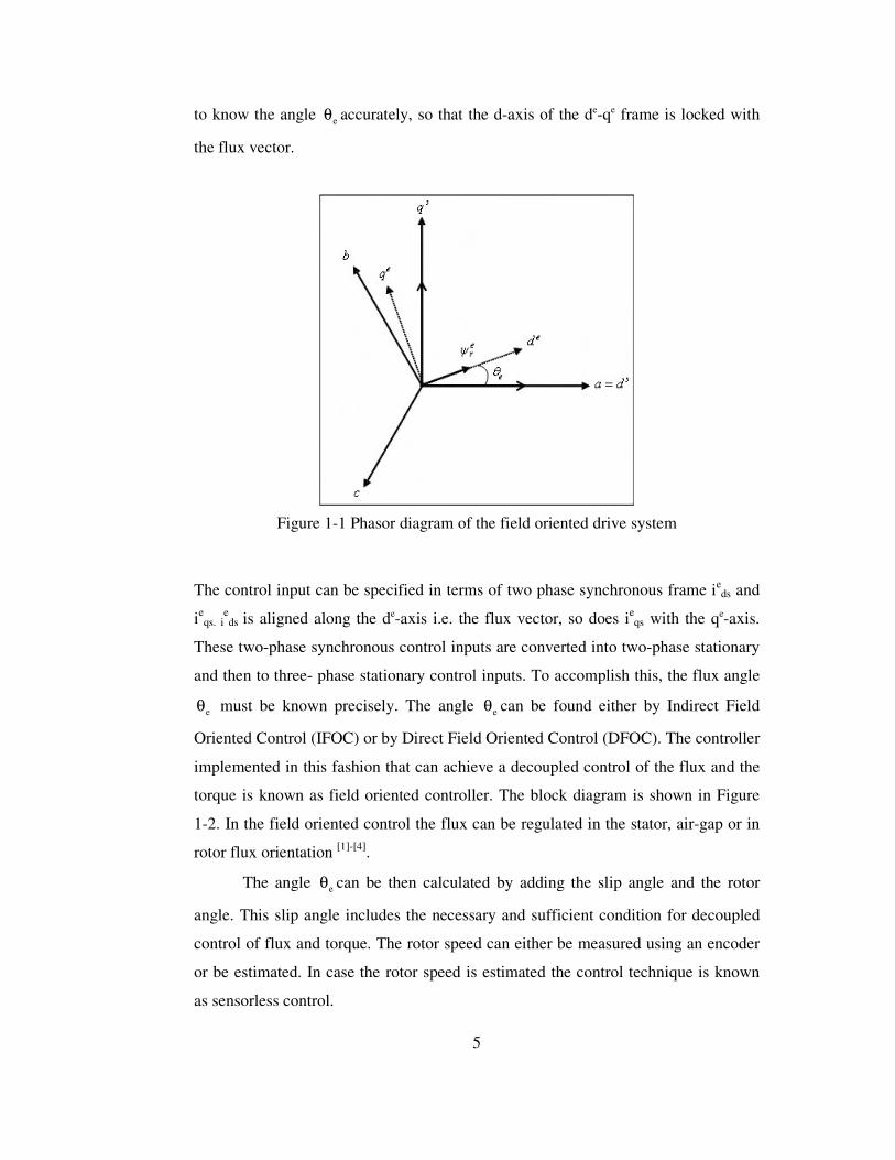
5
to know the angle eθ accurately, so that the d-axis of the de-qe frame is locked with
the flux vector.
Figure 1-1 Phasor diagram of the field oriented drive system
The control input can be specified in terms of two phase synchronous frame ieds and
ieqs. i
eds is aligned along the de-axis i.e. the flux vector, so does ie
qs with the qe-axis.
These two-phase synchronous control inputs are converted into two-phase stationary
and then to three- phase stationary control inputs. To accomplish this, the flux angle
eθ must be known precisely. The angle eθ can be found either by Indirect Field
Oriented Control (IFOC) or by Direct Field Oriented Control (DFOC). The controller
implemented in this fashion that can achieve a decoupled control of the flux and the
torque is known as field oriented controller. The block diagram is shown in Figure
1-2. In the field oriented control the flux can be regulated in the stator, air-gap or in
rotor flux orientation [1]-[4].
The angle eθ can be then calculated by adding the slip angle and the rotor
angle. This slip angle includes the necessary and sufficient condition for decoupled
control of flux and torque. The rotor speed can either be measured using an encoder
or be estimated. In case the rotor speed is estimated the control technique is known
as sensorless control.

6
Figure 1-2 Field oriented induction motor drive system
In this technique the flux angle eθ is classically calculated by means of sensing the
air-gap flux using the flux sensing coils, or can be calculated by estimating the flux
along the (ds-qs) axes using the voltage and current signals.
Figure 1-3 Indirect field oriented drive system
αβi
αβVObserverFlux
αβ
αβ
ψψ
r
s1tan−eθ
Figure 1-4 Direct field oriented drive system

7
1.1.2 Indirect Field Oriented Control
The indirect field oriented control is based on the determination of the slip
frequency, which is a necessary and sufficient condition to guarantee the field
orientation. When the field is once oriented the synchronous speed we is the same as
the instantaneous speed of the rotor flux vector edrψ and de-axis of the de-qe
coordinate system is exactly locked on the rotor flux vector (rotor flux vector
orientation). This facilities the flux control through the magnetizing current edsi by
aligning all the flux along the de-axis while applying the torque-producing
component of the current along the qe-axis. After decoupling the rotor flux and
torque-producing component of the current components, the torque can be
instantaneously controlled by controlling the current eqsi . The requirement to align
the rotor flux along the de-axis of the de-qe coordinate system means that the flux
along the qe-axis must be zero. This means that (1.7) becomes meqrr
eqs L/)iL(i −= and
the current going through the qe-axis of the mutual inductance is zero. Based on this
restriction wsl is:
eds
r
eqs
rsl
ipT
iT
w
−
=
11
1
(1-11)
This relation suggests that flux and torque can be controlled independently by
specifying de-qe axes currents provided that the slip frequency satisfies (1.11) all the
time.
The concept of indirect field oriented control was developed in the history of
AC machine control and has been widely studied by researchers during the last two
decades. Rotor flux orientation is the original and usual choice for the indirect
oriented control. Also the IFOC can be implemented in the stator and air-gap flux
orientation as well. De Doncker introduced this concept in his universal field
oriented controller[5]. In an air-gap flux the slip and flux relations are coupled
equations and the d-axis current does not independently control the flux as it does in
8
the rotor flux orientation. For the constant air-gap flux orientation maximum
produced torque is %20 less than the other two methods[3]. In the stator flux
orientation, the transient reactance is a coupling factor and it varies with the
operating conditions of the machine. In addition, among these methods Nasar shows
that the rotor flux oriented control has linear torque curve[3]. Therefore, the most
commonly used choice for IFO is the rotor flux orientation.
The IFOC is an open-loop feed-forward control in which the slip frequency is
fed-forward guaranteeing the field orientation. This feed-forward control is very
sensitive to the rotor open-circuit time-constant. Therefore, Tr must be known in
order to achieve a decoupled control of torque and flux components by controlling eds
eqs iandi , respectively. When Tr is not set correctly the machine is said to be de-
tuned and the performance will become sluggish due to loss of decoupled control of
torque and flux. The rotor time-constant measurement, its effects of the system and
its tuning to adapt the variations when the machine is operating, has been studied
extensively in the area of IFOC [6-8]. Lorenz, Krishnan and Novotny studied the effect
of temperature and saturation level on the rotor time-constant and stated that it can
reduce the torque capability of the machine and torque/amps of the machine [6-8]. The
de-tuning effect becomes more severe in the field-weakening region. Also, it results
in a steady-state error and, transient oscillations in the rotor flux and torque. Some of
the advanced control techniques such as estimation theory tools and adaptive control
tools are also studied to estimate rotor time-constant and other motor parameters[11-14-
21].
1.1.3 Direct Field Oriented Control
The DFOC and sensorless control relies heavily on accurate flux estimation.
DFOC is most often used for sensorless control, because the flux observer used to
estimate the synchronous speed or angle can also be used to estimate the machine
speed. Investigation of ways to estimate the flux and speed of the induction machine
has been extensively studied in the past two decades. Classically, the rotor flux was
measured by using a special sensing element, such as Hall-effect sensors placed in
the air-gap. An advantage of this method is that additional required parameters, Llr,

9
Lm, and Lr are not significantly affected by changes in temperature and flux level.
However, the disadvantage of this method is that a flux sensor is expensive and
needs special installation and maintenance. Another flux and speed estimation
technique is saliency based with fundamental or high frequency signal injection. One
advantage of saliency technique is that the saliency is not sensitive to actual motor
parameters, but this method fails at low and zero speed level. When applied with
high frequency signal injection, the method may cause torque ripples, vibration and
audible noise [9].
Gabriel avoided the special flux sensors and coils by estimating the rotor flux
from the terminal quantities (stator voltages and currents)[10]. This technique requires
the knowledge of the stator resistance along with the stator-leakage, and rotor-
leakage inductances and the magnetizing inductance. This method is commonly
known as the Voltage Model Flux Observer (VMFO). The stator flux in the
stationary reference frame can be estimated by the equations: sdss
sds
sds irv −=ψ� (1-12)
sqss
sqs
sqs irv −=ψ� (1-13)
Then the rotor flux can be expressed as:
)( sds
sds
m
rsdr iL
LL
σψψ −= (1-14)
)( sqs
sqs
m
rsqr iL
LL
σψψ −= (1-15)
where )L/LL(L r2ms −=σ is the transient leakage inductance.
In this model, integration of the low frequency signals, dominance of stator
IR drop at low speed and leakage inductance variation result in a less precise flux
estimation. Integration at low frequency has been studied and there are three different
alternatives[11]. Estimation of rotor flux from the terminal quantities depends on
parameters such as stator resistance and leakage inductance. The study of parameter
sensitivity shows that the leakage inductance can significantly affect the system

10
performance regarding to stability, dynamic response and utilization of the machine
and the inverter.
The Current Model Flux Observer (CMFO) is an alternative approach to
overcome the problems caused by the changes in leakage inductance and stator
resistance at low speed. In this model flux can be estimated as:
sds
r
msqrr
sdr
r
sdr i
TL
wT
+−−= ψψψ 1� (1-16)
sqs
r
msdrr
sqr
r
sqr i
TL
wT
+−−= ψψψ 1� (1-17)
However, CMFO does not work well at high speeds due to its sensitivity
against the changes in the rotor resistance. Jansen did an extensive study on both
VMFO and CMFO, based on direct field oriented control, discussed the design and
accuracy assessment of various flux observers, and compared and analyzed the
alternative flux observers[12]. To further improve the observer performance, closed-
loop rotor flux observers are proposed which use the estimated stator current error or
the estimated stator voltage error to estimate the rotor flux[12-13]. Lennart proposed
reduced-order observers for this task[14].
1.2 Variable Speed Control Using Advanced Control
Algorithms
There are two issues in motion control of induction machine drives using
field orientation. One is to make the resulting drive system and the controller robust
against parameter deviations and disturbances. The other is to make the system
intelligent e.g. to adjust the control system itself to environment changes and task
requirements. Specifically, even though FOC provides a decoupled control of flux
and torque, a near-instantaneous control of torque for an induction machine drive, for
high performance speed regulation plays an important role, since the command
current *qsi is produced by speed-loop, which feeds the induction machine via the
current regulation to produce the desired torque response. If the speed regulation
loop fails to produce the command current correctly, than the desired torque response

11
will not be produced by the induction machine. In addition, the failure to produce the
correct current command may cause the degradation in slip command as well. As a
result a satisfactory speed regulation is extremely important not only to produce
desired torque performance from the induction machine but also to guarantee the
decoupling between control of torque and flux.
Conventionally, a PI controller has been used for the speed regulation to
generate a command current for the last two decades and accepted by industry
because of its simplicity. Even though a well-tuned PI controller performs well for a
field oriented induction machine during steady-state, the transient speed response of
the machine, especially for the variable speed tracking, is sometimes problematic. In
the last two decades, alternative control algorithms for the speed regulation are
investigated. Among these, fuzzy logic, sliding mode and adaptive nonlinear control
algorithms gain much attention, however these controllers are not in the scope of this
thesis.
A traditional rotor flux oriented induction machine drive offers a control
performance but often requires additional sensors on the machine. This adds to the
cost and complexity of the drive system. To avoid these sensors on the machine,
many different algorithms are proposed in the last three decades to estimate the rotor
flux vector and/or rotor shaft speed. The recent trend in field-oriented control is to
avoid sensors and use algorithms to use the terminal quantities of the machine for the
estimation of the fluxes and speed and they can easily be applied to any induction
machine. Therefore the focus in this study is on these algorithms.
Before looking into individual approaches, the common problems of the
speed and flux estimation are discussed briefly for general field orientation and state
estimation algorithms.
• Parameter sensitivity: One of the most important problem of the
sensorless control algorithms for the field oriented induction machine
drives is insufficient information about the machine parameters which
yield the estimation of some machine parameters along with the
sensorless structure. Among these parameters stator resistance, rotor
resistance and rotor time-constant play more important role than the other
parameters since they are more sensitive to temperature changes. The

12
knowledge of the stator resistance rs, correctly is important to widen the
operation region toward the lower speed range. Since at low speeds the
induced voltage is low and stator resistance drop becomes dominant, the
mismatching of the stator resistance induces instability of the system. On
the other hand errors in determining the actual value of the rotor
resistance rr, may cause both instability of the system and speed
estimation error proportional to rr[15]. Also correct Tr value is vital for the
decoupling factor in IFOC.
• Integration issue: The other important issue regarding to many of the
topologies is the integration process inherited from the induction machine
dynamics. To calculate the state variables of the system, integration
process is needed. However, it is difficult to decide on the initial value
which will not cause the drift of a pure integrator. Usually, to overcome
this problem an integrator is replaced by a low-pass filter.
• Overlapping-loop issues: In a sensorless control system, the control loop
and the speed estimation loop may overlap and these loops influence each
other. As a result, outputs of both of these loops may not be designed
independently; in some bad cases this dependency may influence the
stability or performance of the overall system.
The algorithms, where terminal quantities of the machine are used to estimate
the fluxes and speed of the machine, are categorized in two basic groups. First one is
"the open-loop observer". In a sense it is an on-line model of the machine, which do
not use the feedback correction. Second one is "the closed-loop observer" where the
feedback correction is used along with the machine model itself to improve the
estimation accuracy. These two basic groups can also be subdivided based on the
control method used. These can be summarized as:
• Open-loop observers;
� Current model
� Voltage model
� Cancellation method
� Full-order observer
• Closed-loop observers;

13
� Model Referenced Adaptive Systems (MRAS)
� Kalman filter techniques
� Adaptive observers based on both voltage and current model
� Neural network flux and speed estimators
� Sliding mode flux and speed estimators
Open-loop observers in general use different forms of the induction machine
differential equations. Current model based open-loop observers use the measured
stator currents and rotor velocity[12-14]. The velocity dependency of the current model
is very important since this means that even though using the estimated flux
eliminates the need for the use of a flux sensor, the need for the use of the position
sensor is still there. On the other hand voltage model based open-loop observers use
the measured stator voltage and current as inputs. These types of estimators require a
pure integration that is difficult to implement for low excitation frequencies due to
the offset and initial condition problems. Cancellation method open-loop observers
can be formed by using measured stator voltage, stator current and rotor velocity as
inputs. They use the differentiation to cancel the effect of the integration. However it
suffers from two main drawbacks. One is the need for the derivation which makes
the method more susceptible to noise than the other methods. The other drawback is
the need for the accurate knowledge of the rotor velocity similar to the current
model. A full-order open-loop observer on the other hand can be formed using only
the measured stator voltage and rotor velocity as inputs where the stator current
appears as an estimated quantity. Because of its dependency on the stator current
estimation, the full-order observer will not exhibit better performance than the
current model. Furthermore, parameter sensitivity and observer gain are the problems
to be tuned in a full-order observer design[16]. These open-loop observer structures
are all based on the induction machine model and they do not employ any feedback.
Therefore, they are quite sensitive to parameter variations, which yield the estimation
of some machine parameters along with the sensorless structure.
On the other hand some kind of feedback may be helpful to produce more
robust structures against parameter variations. For this purpose many closed-loop
topologies are proposed using different induction machine models and control
14
methods. Among these MRAS attracts attention and several different algorithms are
produced. In MRAS, in general a comparison is made between the outputs of two
estimators. The estimator which does not contain the quantity to be estimated can be
considered as a reference model of the induction machine. The other one, which
contains the estimated quantity, is considered as an adjustable model. The error
between these two estimators is used as an input to an adaptation mechanism. For
sensorless control algorithms most of the times the quantity which differs the
reference model from the adjustable model is the rotor speed. When the estimated
rotor speed in the adjustable model is changed in such a way that the difference
between two estimators converges to zero asymptotically, the estimated rotor speed
will be equal to the actual rotor speed. The basics of the analysis and design of
MRAS are discussed by Vas, and Trzynadlowski [2, 17]. The voltage model here is
assumed as reference model, the current model, however, is assumed as the
adjustable model and the estimated rotor flux is assumed as the reference parameter
to be compared[15, 18, and 19]. Similarly speed estimators, proposed here, are based on the
MRAS, and a secondary variable is introduced as the reference quantity by putting
the rotor flux through a first-order delay instead of a pure integration to nullify the
offset by Robyns and Frederique[16]. However, their algorithm produces inaccurate
estimated speed when the excitation frequency goes below a certain level. In addition
these algorithms suffer from the machine parameter uncertainties because of the
reference model since the parameter variation in the reference model cannot be
corrected. An alternative MRAS based on the electromotive force rather than rotor
flux as reference quantity for speed estimation is suggested in order to overcome the
integration problem[19, 21]. Further, another new auxiliary variable is introduced which
represents the instantaneous reactive power for maintaining the magnetizing current.
In this MRAS algorithm stator resistance disappear from equations making the
algorithm robust against that parameter. Zhen proposed an interesting MRAS
structure that is built with two mutual MRAS schemes[22]. In this structure, the
reference model and the adjustable models are interchangeable. For rotor speed
estimation, one model is used as reference model and other model is used as
adjustable model. The pure integration is removed from reference model. For stator
resistance estimation, however, these models switch their roles.

15
1.3 Overview of the Chapters This thesis is organized as follows:
Chapter 1 is devoted to vector control fundamentals. Indirect and direct
control methods are introduced and sensorless direct field oriented control using flux
and open-loop speed estimators are discussed briefly.
In Chapter 2, generalized dynamic mathematical model of the induction
motor in different reference frames are presented.
Chapter 3 presents the theoretical background of Space Vector Pulse Width
Modulation (SVPWM) in detail. The results of simulation and the DSP
implementation of this theory are illustrated.
Chapter 4 includes the detailed description of the flux estimation with the
assumption that the rotor current is zero. The method of the flux estimation is given
when the measured speed signal is no longer available. The speed estimation method
based upon the mathematical model of the induction motor is also given in this
chapter.
Chapter 5 presents the obtained simulated and experimental results of the
drive system for both open-loop and closed-loop cases.
In Chapter 6 implementation method for vector control is introduced. The
experimental setup used for testing the proposed sensorless drive system is
described.
Chapter 7 summarizes the thesis and concludes the performance of the vector
controlled induction motor.
16
2 INDUCTION MACHINE MODELLING
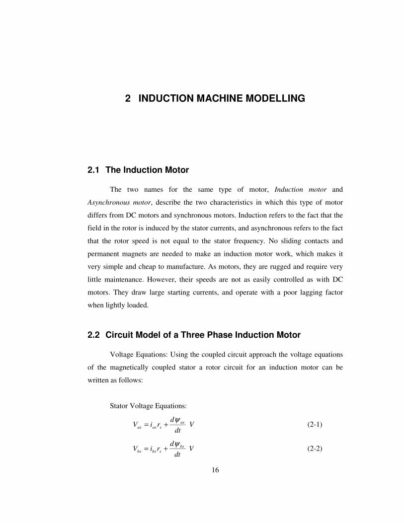
2.1 The Induction Motor
The two names for the same type of motor, Induction motor and
Asynchronous motor, describe the two characteristics in which this type of motor
differs from DC motors and synchronous motors. Induction refers to the fact that the
field in the rotor is induced by the stator currents, and asynchronous refers to the fact
that the rotor speed is not equal to the stator frequency. No sliding contacts and
permanent magnets are needed to make an induction motor work, which makes it
very simple and cheap to manufacture. As motors, they are rugged and require very
little maintenance. However, their speeds are not as easily controlled as with DC
motors. They draw large starting currents, and operate with a poor lagging factor
when lightly loaded.
2.2 Circuit Model of a Three Phase Induction Motor
Voltage Equations: Using the coupled circuit approach the voltage equations
of the magnetically coupled stator a rotor circuit for an induction motor can be
written as follows:
Stator Voltage Equations:
Vdt
driV as
sasas
ψ+= (2-1)
Vdt
driV bs
sbsbs
ψ+= (2-2)

17
Vdt
driV cs
scscs
ψ+= (2-3)
Rotor Voltage Equations:
Vdt
driV ar
rarar
ψ+= (2-4)
Vdt
driV br
rbrbr
ψ+= (2-5)
Vdt
driV cr
rscrcr
ψ+= (2-6)
Flux Linkage Equations: In matrix notation, the flux linkages of the stator and
rotor windings, in terms of the winding inductances and currents, may be written
compactly as
turnsWbi
i
LL
LLabcr
abcs
abcrr
abcrs
abcsr
abcss
abcr
abcs .�
�
���
���
���
�=
���
�
���
�
ψψ
(2-7)
where
( )( )
( )( )t
crbrarabcr
tcsbsas
abcs
tcrbrar
abcr
tcsbsas
abcs
iiii
iiii
,,
,,
,,
,,
=
=
=
=
ψψψψ
ψψψψ
(2-8)
and the superscript (t) denotes the transpose of the array.
The sub-matrices of the stator-to-rotor and rotor-to-rotor winding inductances
are of the form:
H
LLLL
LLLL
LLLL
L
H
LLLL
LLLL
LLLL
L
rrrrmrm
rmrrrrm
rmrmrrrabcrr
sslssmsm
smsslssm
smsmsslsabcss
���
�
�
���
�
�
++
+=
���
�
�
���
�
�
++
+=
(2-9)

18
Those of the stator to rotor mutual inductances are dependent on the rotor angle, that
is:
HLLL
rrr
rrr
rrr
srtabc
rsabcsr
�������
�
�
�������
�
�
��
�
� −��
�
� +
��
�
� +��
�
� −
��
�
� −��
�
� +
==
θπθπθ
πθθπθ
πθπθθ
cos3
2cos
32
cos
32
coscos3
2cos
32
cos3
2coscos
][ (2-10)
where Lls is the per phase stator winding leakage inductance, Llr is the per phase rotor
winding leakage inductance, Lss is the self inductance of the stator winding, Lrr is the
self inductance of the rotor winding, Lsm is the mutual inductance between stator
windings, Lrm is the mutual inductance between rotor windings, and Lsr is the peak
value of the stator to rotor mutual inductance.
Note that the idealized machine is described by six first-order differential
equations, one for each winding. These differential equations are coupled to one
another through the mutual inductance between the windings. In particular, the stator
to rotor coupling terms vary with time. Mathematical transformations like the dq or
� can facilitate the computation of the transient solution of the above induction
motor model by transforming the differential equations with time-varying
inductances to differential equations with constant inductances.
2.2.1 Machine Model in Arbitrary dq0 Reference Frame
The idealized three-phase induction machine is assumed to have symmetrical
air-gap. The dq0 reference frames are usually selected on the basis of conveniences
or computational reduction. The two commonly used reference frames in the analysis
of induction machine are the stationary and synchronously rotating frames. Each has
an advantage for some purpose. In the stationary rotating reference, the dq variables
of the machine are in the same frame as those normally used for the supply network.
In the synchronously rotating frame, the dq variables are steady in steady state. Here,

19
firstly the equations of the induction machine in the arbitrary reference frame which
is rotating at a speed of (w) in the direction of the rotor rotation will be derived.
Those if the induction machine in the stationary frame can then be obtained by
setting w=0, and those for the synchronously rotating frame are obtained by setting
w=we. The relationship between the abc quantities and dq0 quantities of a reference
frame rotating at an angular speed, w, is shown in Figure 2-1.
Figure 2-1 Relationship between abc and arbitrary dq0
The transformation equation from abc to this qd0 reference frame is given by:
[ ]���
�
�
���
�
�
=���
�
�
���
�
�
0
0
0
)(
f
f
f
T
f
f
f
b
a
qdd
q
θ (2-11)
where the variable f can be the phase voltages, current, or flux linkages of the
machine. The transformation angle, �(t), between the q-axis of the reference frame
rotating at a speed of w and the a-axis of the stationary stator winding may be
expressed as:
+=t
radelecdttwt0
..)0()()( θθ (2-12)

20
Likewise, the rotor angle, �r(t), between the axes of the stator and rotor a-phases for a
rotor rotating with speed wr (t) may be expressed as:
+=t
rrr radelecdttwt0
..)0()()( θθ (2-13)
2.2.1.1 qd0 Voltage Equations In matrix notation, the stator winding abc voltage equations can be expressed
as:
abcs
abcs
abcs
abcs irpv += ψ (2-14)
Applying the transformations (Clarke and Park) to the voltage, current and
flux linkages (2.14) becomes
[ ] [ ] [ ] [ ] [ ] [ ]0100
0100
0 )()()()( qdsqdsqd
qdsqdqd
qds iTrTTpTv −− += θθψθθ (2-15)
solving the equation above it becomes:
00000
000001010
qds
qds
qds
qds
qds irpwv ++
���
�
�
���
�
�
−= ψψ (2-16)
where
���
�
�
���
�
�
==100010001
0s
qds rrand
dtd
wθ
(2-17)
Likewise, the rotor voltage equation becomes:
0000
000001010
)( qdr
qdr
qdr
qdsrr
qdr irpwwv ++
���
�
�
���
�
�
−−= ψψ (2-18)

21
2.2.1.2 qd0 Flux Linkage Relation
The stator qd0 flux linkages are obtained by applying Tqd0 (�) to the stator abc
flux linkages in (2.7).
)()]([ 00 abc
srabcsr
abcss
abcssqd
qds iLiLT += θψ (2-19)
skipping the transformation steps the stator and the rotor flux linkage relationships
can be expressed compactly:
��������
�
�
��������
�
�
��������
�
�
��������
�
�
+′+′
++
=
��������
�
�
��������
�
�
r
dr
qr
s
ds
qs
m
mlrm
mlrm
ls
mmsl
mmsl
r
dr
qr
s
ds
qs
i
i
i
i
i
i
L
LLL
LLL
L
LLL
LLL
0
0
0
0
00000000000000000000000000
ψψψψψψ
(2-20)
Substituting (2.20) into voltage equations and then grouping q, d, 0, and �
terms in the resulting voltage equations, we obtain the voltage equations that suggest
the equivalent circuit shown in Figure 2-2.
+ −
qsE
qsisr sL1
wds ×ψ
+−
qrE '
rr 'rL 1')(' rdr ww −×ψ
dri'
qsv+
− qrv'+
−
axisq −
Figure 2-2 Model of an induction machine in the arbitrary reference frame

22
+ −
dsE
dsisr sL1
wqs ×ψ
+−
drE '
rr 'rL 1')(' rqr ww −×ψ
dri'
dsv+
− drv'+
−
axisd −
mL
Figure 2-3 Model of an induction machine in the arbitrary reference frame
2.2.1.3 qd0 Torque Equations
The sum of the instantaneous input power to all six windings of the stator and
rotor is given by :
Wivivivivivivp crcrbrbrararcscsbsbsasasin ′′+′′+′′+++= (2-21)
in terms of dq quantities
Wivivivivivivp rrdrdrqrqrssdsdsqsqsin )22(23
0000 ′′+′′+′′+++= (2-22)
Using stator and rotor voltages to substitute for the voltages on the right hand
side of (2.22), we obtain three kinds of terms: iwandpiri ψψ ,,2 . (i2r) terms are the
cupper losses. The (ip�) terms represent the rate of exchange of magnetic field
energy between windings. The electromechanical torque developed by the machine is
given by the sum of the (w�i ) terms divided by mechanical speed, that is:
[ ] Nmiiwwiiwwp
T drqrqrdrrdsqsqsdsr
em ))(()(22
3 ′′−′′−+−= ψψψψ (2-23)
using the flux linkage relationships, Tem can also be expressed as follows:
[ ] NmiiwwiiwwP
T drqrqrdrrdsqsqsdsr
em ))(()(22
3 ′′−′′−+−= ψψψψ (2-24)
Using the flux linkage relationships, one can show that
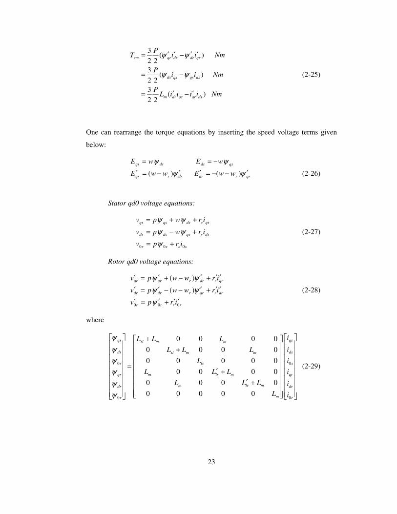
23
NmiiiiLP
NmiiP
NmiiP
T
dsqrqsdrm
dsqsqsds
qrdrdrqrem
)(22
3
)(22
3
)(22
3
′−′=
−=
′′−′′=
ψψ
ψψ
(2-25)
One can rearrange the torque equations by inserting the speed voltage terms given
below:
qrrdrdrrqr
qsdsdsqs
wwEwwE
wEwE
ψψψψ
′−−=′′−=′−==
)()( (2-26)
Stator qd0 voltage equations:
ssss
dssqsdsds
qssdsqsqs
irpv
irwpv
irwpv
000 +=
+−=
++=
ψψψψψ
(2-27)
Rotor qd0 voltage equations:
rrrr
drrqrrdrdr
qrrdrrqrqr
irpv
irwwpv
irwwpv
000
)(
)(
′′+′=′
′′+′−−′=′
′′+′−+′=′
ψψψψψ
(2-28)
where
��������
�
�
��������
�
�
��������
�
�
��������
�
�
+′+′
++
=
��������
�
�
��������
�
�
r
dr
qr
s
ds
qs
m
mlrm
mlrm
ls
mmsl
mmsl
r
dr
qr
s
ds
qs
i
i
i
i
i
i
L
LLL
LLL
L
LLL
LLL
0
0
0
0
00000000000000000000000000
ψψψψψψ
(2-29)

24
Torque Equation:
[ ] NmiiwwiiwwP
T drqrqrdrrdsqsqsdsr
em ))(()(22
3 ′′−′′−+−= ψψψψ (2-30)
2.2.2 qd0 Stationary and Synchronous Reference Frames
There is seldom a need to simulate an induction machine in the arbitrary
rotating reference frame. But it is useful to convert a unified model to other frames.
The most commonly used ones are, two marginal cases of the arbitrary rotating
frame, stationary reference frame and synchronously rotating frame. For transient
studies of adjustable speed drives, it is usually more convenient to simulate an
induction machine and its converter on a stationary reference frame. Moreover,
calculations with stationary reference frame are less complex due to zero frame
speed (some terms cancelled). For small signal stability analysis about some
operating condition, a synchronously rotating frame which yields steady values of
steady-state voltages and currents under balanced conditions is used.
Since we have derived the equations of the induction machine for the general
case, that is in the arbitrary rotating reference frame, the equations of the machine in
the stationary and synchronously rotating reference frame, w to zero and we,
respectively. To distinguish these two frames from each other, an additional
superscript will be used, s for stationary frame variables and e for synchronously
rotating frame variables.
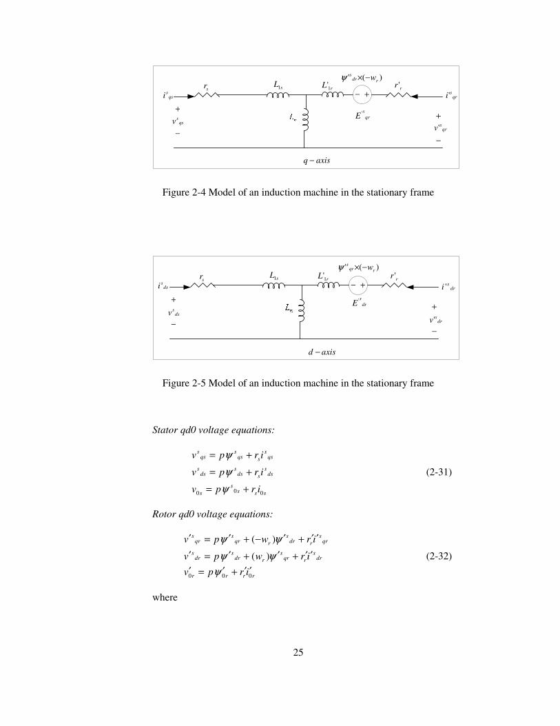
25
qssi
sr sL1
+−
qrs
E '
rr 'rL 1')(' rdr
s w−×ψ
qrsi'
qssv+
− qrsv'
+
−
axisq −
Figure 2-4 Model of an induction machine in the stationary frame
dssi
sr sL1
+−
drs
E '
rr 'rL 1')(' rqr
s w−×ψ
drsi '
dssv
+
− drsv'
+
−
axisd −
Figure 2-5 Model of an induction machine in the stationary frame
Stator qd0 voltage equations:
ssss
s
dss
sdss
dss
qss
sqss
qss
irpv
irpv
irpv
000 +=
+=
+=
ψψψ
(2-31)
Rotor qd0 voltage equations:
rrrr
drs
rqrs
rdrs
drs
qrs
rdrs
rqrs
qrs
irpv
irwpv
irwpv
000
)(
)(
′′+′=′′′+′+′=′
′′+′−+′=′
ψψψ
ψψ (2-32)
where

26
��������
�
�
��������
�
�
��������
�
�
��������
�
�
+′+′
++
=
��������
�
�
��������
�
�
r
drs
qrs
s
dss
qss
m
mlrm
mlrm
ls
mmsl
mmsl
r
drs
qrs
s
dss
qss
i
i
i
i
i
i
L
LLL
LLL
L
LLL
LLL
0
0
0
0
00000000000000000000000000
ψψψψψψ
(2-33)
Torque Equation:
NmiiiiLP
NmiiP
NmiiP
T
dss
qrs
qss
drs
m
dss
qss
qss
dss
qrs
drs
drs
qrs
em
)(22
3
)(22
3
)(22
3
′−′=
−=
′′−′′=
ψψ
ψψ
(2-34)
The equivalent induction machine circuit and induction machine equations in the
synchronous reference frame are given in (2.35-2.38) and Figure 2-6, Figure 2-7. 3-
phase AC quantities are simulated in both stationary frame and synchronously
rotating frame.
qsei
sr sL1
+−
qrs
E '
rr 'rL 1')(' redr
e ww −×ψ
qrei'
qsev
+
− qrev'+
−
axisq −
+−
−
qseE
Figure 2-6 Model of an induction machine in the synchronous frame

27
dsei
sr sL1
+−
dre
E '
rr 'rL 1')(' reqr
e ww −×ψ
drei'
dsev+
− drev'+
−
axisd −
+ −
dseE
Figure 2-7 Model of an induction machine in the synchronous frame
Stator qd0 voltage equations:
ssss
dse
sqse
edse
dse
qse
sdse
eqse
qse
irpv
irwpv
irwpv
000 +=+−=
++=
ψψψψψ
(2-35)
Rotor qd0 voltage equations:
rrrr
dre
rqre
redre
dre
qre
rdre
reqre
qre
irpv
irwwpv
irwwpv
000
)(
)(
′′+′=′′′+′−−′=′
′′+′−+′=′
ψψψψψ
(2-36)
where
��������
�
�
��������
�
�
��������
�
�
��������
�
�
+′+′
++
=
��������
�
�
��������
�
�
r
dre
qre
s
dse
qse
m
mlrm
mlrm
ls
mmsl
mmsl
r
dre
qre
s
dse
qse
i
i
i
i
i
i
L
LLL
LLL
L
LLL
LLL
0
0
0
0
00000000000000000000000000
ψψψψψψ
(2-37)
Torque Equations:
NmiiiiLP
NmiiP
NmiiP
T
dse
qre
qse
dre
m
dse
qse
qse
dse
qre
dre
dre
qre
em
)(22
3
)(22
3
)(22
3
′−′=
−=
′′−′′=
ψψ
ψψ
(2-38)

28
3 PULSE WIDTH MODULATION with SPACE VECTOR THEORY
3.1 Inverters Three phase inverters, supplying voltages and currents of adjustable
frequency and magnitude to the stator, are important elements of adjustable speed
induction motor drive systems. Inverters with semiconductor power switches are d.c.
to a.c. static power converters. Depending on the type of d.c. source supplying the
inverter, they can be classified as voltage fed inverters (VFI) or current fed inverters
(CFI). In practice, the d.c. source is usually a rectifier, typically of the three phase
bridge configuration, with d.c. link connected between the rectifier and the inverter.
The d.c. link is a simple inductive, capacitive, or inductive-capacitive low-pass filter,
since neither the voltage across a capacitor nor the current through an inductor can
change instantaneously. A capacitive-output d.c. link is used for a VFI and an
inductive-output link is employed in CFI. VFIs can be either voltage or current
controlled. In a voltage-controlled inverter, it is the frequency and magnitude of the
fundamental of the output voltage that is adjusted. Feed-forward voltage control is
employed, since the inverter voltage is dependent only on the supply voltage and the
states of the inverter switches, and, therefore, accurately predictable. Current
controlled VFIs require sensors of the output currents which provide the necessary
control feedback. The type of semiconductor power switch used in an inverter
depends on the volt-ampere rating of the inverter, as well as on other operating and
economic considerations, such as switching frequency or cost of the system. Taking
into account the transient and steady state requirements, we have used 1200V, 40A
IGBT switches. With appropriate heat sink, we can rise to 20 KHz, however at 10
KHz, switching losses and conduction losses become equal moreover, complex

29
mathematical algorithms require much time. Thus 10 KHz is selected as the
switching frequency in our algorithms.
3.1.1 Voltage Source Inverter (VFI) A diagram of the power circuit of a three phase VFI is shown in the Figure
3-1. The circuit has bridge topology with three branches (phases), each consisting of
two power switches and two freewheeling diodes. The inverter here is supplied from
an uncontrolled, diode-based rectifier, via d.c. link which contains an LC filter in the
inverted configuration. It allows the power flow from the supply to the load only.
Power flow cannot be reversed, if the load is to feed the power back to the supply
due to the diode rectifier structure at the input side of the dc link. Therefore, in drive
systems where the VFI-fed motor may not operate as a generator, a more complex
supply system must be used. These involve either a braking resistance connected
across the d.c. link or replacement of the uncontrolled rectifier by a dual converter.
The inverter may be supported with braking resistance connected across the d.c. link
via a free wheeling diode and a transistor. When the power flow is reversed it is
dissipated in the braking resistor putting the system into dynamic braking mode of
operation.
Figure 3-1 Circuit diagram of VFI

30
Because of the constraint that the input lines must never be shorted and the output
current must be continuous a voltage fed inverter can assume in operation only eight
distinct topologies. They are shown in Figure 3-2 and Figure 3-3. Six out of these
eight topologies produce a non zero output voltage and are known as non-zero
switching states and the remaining two topologies produce zero output and are
known as zero switching state.
Figure 3-2 Three phase inverter with switching states

31
Figure 3-3 Eight switching state topologies of a voltage source inverter

32
3.2 Voltage Space Vectors Space vector modulation for three leg VFI is based on the representation of the three
phase quantities as vectors in two-dimensional (ds-qs) plane. Considering the first
switching state in Figure 3-4, line-to-line voltages are given by:
Vab = Vs Vbc = 0 Vca = -Vs
Figure 3-4 First switching state –V1
This can be represented in (ds-qs) plane as shown in Figure 3-5 where Vab, Vbc and
Vca are the three line voltage vectors displaced 120° in space. The effective voltage
vector generated by this topology is represented as V1 (pnn) in Figure 3-5. Here
(pnn) refers to the three leg /phases a, b, c being either connected to the positive dc
rail (p) or to the negative dc rail (n). For the first switching state V1, phase a
connected to positive dc rail and phases b and c are connected to negative dc rail.
Similar to the V1, six non zero voltage vectors can be shown as in Figure 3-6. The
tips of these vectors form a regular hexagon. We define the area enclosed by two
adjacent vectors, within the hexagon, as a sector.

33
Figure 3-5 Representation of topology 1 in (ds-qs) plane
Figure 3-6 Non-zero voltage vectors in (ds-qs) plane
The first and the last two topologies of Figure 3-3 are zero state vectors. The output
line voltages in these topologies are zero.
Vab=0
Vbc=0
Vca=0
These are represented as vectors which have zero magnitude and hence are referred
as zero switching state vectors. They are represented with dot at the origin instead of
vectors as shown in Figure 3-7.

34
Figure 3-7 Representation of the zero voltage vectors in (ds-qs) plane
3.2.1 SVPWM Application to the Static Power Bridge and
Implementation Using DSP Platform
In the case of AC drive applications, sinusoidal voltage sources are not used as
explained before. Instead, they are replaced by 6 power IGBTs which act as on/off
switches to the rectified DC bus voltage. The aim is to create sinusoidal current in
the windings to generate rotating field. Owing to the inductive nature of the phases, a
pseudo sinusoidal current is created by modulating the duty-cycle of the power
switches. The switches (IGBT) shown in the Figure 3-2 are activated by signals (a, b,
c) and their complement values. Eight different combinations are available with this
three phase VFI including two zero states. It is possible to express each phase to
neutral voltages, for every switching combinations of IGBT’s as listed in Table 3-1.
Table 3-1 Power Bridge Output Voltages (VAN, VBN, VCN)
Switch Positions Phase Voltages S1 S2 S3 VAN VBN VCN 0 0 0 0 0 0 0 0 1 -Vdc/3 -Vdc/3 2Vdc/3 0 1 0 -Vdc/3 2Vdc/3 -Vdc/3 0 1 1 -2Vdc/3 Vdc/3 Vdc/3 1 0 0 2Vdc/3 -Vdc/3 -Vdc/3 1 0 1 Vdc/3 -2Vdc/3 Vdc/3 1 1 0 Vdc/3 Vdc/3 -2Vdc/3 1 1 1 0 0 0

35
In field oriented control algorithm, the control variables are expressed in rotating
frame. The current vector Isref that directly controls the torque is transformed in a
voltage vector by the inverse Park transform. This voltage reference is expressed in
the (ds-qs) frame. Using this transformation three phase voltages (VAN, VBN, VCN) and
the reference voltage vector are projected in the (ds-qs) frame. The expression of the
three phase voltages in the (ds-qs) frame are given by general Clarke transformation:
���
�
�
���
�
�
����
�
�
����
�
�
−
−−=
���
�
���
�
CN
BN
AN
ssq
ssd
V
V
V
V
V
23
23
0
21
21
1
32
(3.1)
Since only 8 combinations are possible for the power switches, Vssd, Vs
sq can also
take finite number of values in the (ds-qs) frame (Table 3-2) according to the IGBT
command signals (a, b, c).
Table 3-2 Stator Voltages in (ds-qs) frame and related Voltage Vector
Switch Positions (ds-qs) frame Voltages S1 S2 S3 Vs
sd Vsqs Vectors
0 0 0 0 0 V0 0 0 1 -Vdc/3 -Vdc/�3 V1 0 1 0 -Vdc/3 Vdc/�3 V2 0 1 1 -2Vdc/3 0 V3 1 0 0 2Vdc/3 0 V4 1 0 1 Vdc/3 -Vdc/�3 V5 1 1 0 Vdc/3 Vdc/�3 V6 1 1 1 0 0 V7
The eight voltage vectors re-defined by the combination of the switches are
represented in Figure 3-8.

36
Figure 3-8 Voltage vectors
Given a reference voltage (coming from the inv. Park transform), the following step
is used to approximate this reference voltage by the above defined eight vectors. The
method used to approximate the desired stator reference voltage with only eight
possible states of switches combines adjacent vectors of the reference voltage and
modulates the time of application of each adjacent vector. In Figure 3-9, the
reference voltage Vsref is in the third sector and the application time of each adjacent
vector is given by:
(3.2)
66
44
064
VTT
VTT
V
TTTT
sref
��+=
++=

37
Figure 3-9 Projection of the reference voltage vector
The determination of the amount of times T4 and T6 is given by simple projections:
(3.3)
Finally, with the (ds-qs) component values of the vectors given in Table 3-2, the
duration periods of application of each adjacent vector is:
)33(24
ssq
ssd
dc
VVVT
T = (3.4)
)36s
sqdc
VVT
T = (3.5)
The rest of the period spent in applying the null vector (T0=T-T6-T4). For every
sector, commutation duration is calculated. The amount of times of vector
application can all be related to the following variables:
)60(
)30cos(
0
44
06
6
tg
Vx
xVTT
V
VTT
V
ssq
ssd
ssq
=
+=
=
�
�

38
(3.6)
In the previous example for sector 3, T4 = -Z and T6 = X. Extending this logic, one
can easily calculate the sector number belonging to the related reference voltage
vector. The following basic algorithm helps to determine the sector systematically.
If X > 0 then A=1 else A=0
If Y > 0 then B=1 else B=0
If Z > 0 then C=1 else C=0
Sector = A+2B+4C
The duration of the sector boundary vectors application can be determined as
follows:
sector
1: t1= Z t2= Y
2: t1= Y t2=-X
3: t1=-Z t2= X
4: t1=-X t2= Z
5: t1= X t2=-Y
6: t1=-Y t2=-Z
Saturations
If (t1+ t2) > PWMPRD then
t1sat = (t1/ t1+t2)*PWMPRD
t2sat = (t2/ t1+t2)*PWMPRD
The third step is to compute the three necessary duty-cycles. This is shown below:
ssd
ssq
ssd
ssq
ssq
VVZ
VVY
VX
23
23
23
23
3
−=
+=
=
2boncon
1aonbon
21aon
ttt
ttt2
ttPWMPRDt
+=+=
−−=

39
The last step is to assign the right duty-cycle (txon) to the right motor phase (in other
words, to the right CMPRx) according to the sector. Table 3-3 below depicts this
determination.
Table 3-3 Assigned duty cycles to the PWM outputs
1 2 3 4 5 6 CMPR1 tbon taon taon tcon tbon tcon CMPR2 taon tcon tbon tbon tcon taon CMPR3 tcon tbon tcon taon taon tbon
3.3 Simulation and Experimental Results of SVPWM
The SVPWM algorithm implemented in this thesis by DSP is simulated before
proceeding through the experimental works to verify its results. In the first
simulation, SVPWM algorithm is simulated step-by-step and all the software
variables in the algorithm are compared with the experimental DSP program outputs.
It is shown that both of the results are the same, and correct.

40
Figure 3-10 Simulated waveforms of duty cycles, ( taon, tbon,tcon )
Figure 3-11 Sector numbers of voltage vector
In Figure 3-10 duty cycles of two PWM switches are shown ( taon, tbon,tcon). In Figure
3-11 sector numbers of the rotating reference voltage vector is given. Note that the
order of the sectors is the same as in Figure 3-11 of a vector rotating in
counterclockwise direction in Figure 3-8 (sectors 3-1-5-4-6-2).
The experimental outputs confirm the theoretical and simulation outputs.
Given two reference voltage vectors associated with the reference currents and

41
torque requirement, SVPWM software parameters are observed and compared with
the simulated ones. The Figure 3-12 shows two phases outputs of SVPWM in a large
time scale. When zoomed into Figure 3-12 as seen in Figure 3-13 one can see the
symmetrical SVPWM in a small timescale. A SVPWM designer must check the
correctness of the six PWM outputs generated by this SVPWM module. A simple
low–pass filter RC circuit may be used to filter out the high frequency components.
The R and C values (or the time-constant) are chosen for a desired cut–off frequency
(fc) using the following equation:
Time-constant = RC = 1/2fc
For example, R = 1.8 k. and C = 100 nF, gives fc = 884.2 Hz. This cut–off
frequency has to be lower than the PWM frequency. This low–pass filter is
connected to the PWM pins of the LF2407 EVM, the filtered version of the PWM
signals are monitored by oscilloscope. The waveforms shown on the oscilloscope
(Figure 3-14, Figure 3-15) should be the same as the one shown in Figure 3-10.
Figure 3-12 SVPWM outputs of two phases
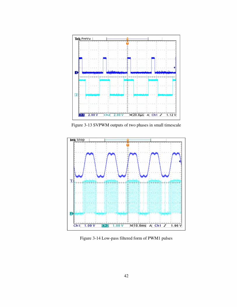
42
Figure 3-13 SVPWM outputs of two phases in small timescale
Figure 3-14 Low-pass filtered form of PWM1 pulses

43
Figure 3-15 Low-pass filtered form of PWM1 and PWM5 pulses

44
4 FLUX AND SPEED ESTIMATION FOR SENSORLESS DIRECT FIELD ORIENTED
CONTROL OF INDUCTION MACHINE
In this chapter, observers configured for direct field-orientation (DFO) are
investigated. The field orientation is implemented in two ways as Direct Field
Orientation and Indirect Field Orientation. The basic difference of these methods
underlies in the manner of detecting the synchronous speed. In IFO, the slip angle is
computed and added to the rotor speed to find the synchronous speed. One must
calculate, therefore, the slip-angle and estimate the rotor angle. In the current model
employed in the IFO, d-q axes stator currents and precise rotor time-constants are
needed to find the slip angle. On the other hand, in DFO, the synchronous speed is
computed from the ratio of dq-axes fluxes.
4.1 Flux Estimation
Flux estimator used in this chapter can compute both the synchronous speed
and the rotor speed. The logic underlying this flux observer is basically an advanced
voltage model approach in which integration of the back-emf is calculated and
compensated for the errors associated with pure integrator and stator resistance Rs
measurement at low speeds. At high speeds, the voltage model provides an accurate
stator flux estimate because the machine back emf dominates the measured terminal
voltage. However, at low speeds, the stator IR drop becomes significant, causing the
accuracy of the flux estimate to be sensitive to the estimated stator resistance. Due to
this effect, at low excitation frequencies flux estimation based upon voltage model
are generally not capable of achieving high dynamic performance at low speeds [12].
Consequences of these problems are compensated with the addition of a closed-loop
in the flux observer. Basically, the fluxes obtained by current model are compared

45
with those obtained by the voltage model with reference to the current model, or the
current model with reference to the voltage model according to the range in which
one of these models is superior to other [23]. In this flux observer the voltage model is
corrected by the current model through a basic PI block. In the end, the stator fluxes
are used to obtain rotor fluxes and rotor flux angle. The overall observer structure is
given below.
4.1.1 Estimation of the Flux Linkage Vector
Most of the sensorless control schemes rely directly or indirectly on the
estimation of the stator flux linkage vector, ψs being defined as the time integral of
the induced voltage,
0
,
)0(, ssoffsss
vs
uiRudt
dψψ
ψ=+−= (4-1)
where, uoff represents all disturbances such as offsets, unbalances and other errors
present in the estimated induced emf. A major source of error in the emf is due to the
changes in the model parameter Rs. The estimation of the flux vectors requires the
integration of (4.1) in real-time. The integrator, however, will have an infinite gain at
zero frequency, and the unavoidable offsets contained in the integrator input then
make its output gradually drift away beyond limits.
4.1.1.1 Flux Estimation in Continuous Time
The rotor flux linkage dynamics in synchronously rotating reference frame
(w=we=wψr) being as;
ieqrre
iedr
r
eds
r
mie
dr wwiL
dtd ,,
,
)(1 ψψ
ττψ −+−= (4-2)

46
iedrre
ieqr
r
eqs
r
mie
qr wwiL
dt
d ,,,
)(1 ψψττ
ψ−+−= (4-3)
where Lm is the magnetizing inductance (H), τr=Lr/Rr is the rotor time-constant (sec),
and wr is the electrical angular velocity of the rotor (rad/sec). In the current model,
the total rotor flux-linkage is aligned with the d-axis component, and hence;
0,
,,
=
=ie
qr
iedr
ier
ψψψ
Substitution of ψqr=0 into (4-2) and (4-3) yields the oriented rotor flux dynamics as;
iedr
r
eds
r
mie
dr iL
dtd ,
, 1 ψττ
ψ −= (4-4)
0, =ie
qrψ (4-5)
Note that (4-4) and (4-5) are the commonly recognized forms of the rotor flux vector
equations. When, the rotor flux linkages in (4-4) and (4-5) undergoes the inverse
park transformation in the stationary reference frame the result becomes.
)cos()sin()cos( ,,,,rrr
iedr
ieqr
iedr
isdr ψψψ θψθψθψψ =−= (4-6)
)sin()sin()cos( ,,,,rrr
iedr
iedr
ieqr
isqr ψψψ θψθψθψψ =+= (4-7)
where θψr is the rotor flux angle (rad). The stator flux linkages in stationary reference
frame are then computed using (4-6) and (4-7) as;
isdr
r
msds
r
mrssdrm
sdss
isds L
Li
LLLL
iLiL ,2
, ψψ +���
�
� −=+= (4-8)
isqr
r
msqs
r
mrssqrm
sqs
isqs L
Li
LLLL
iLiL ,2
, ψψ +���
�
� −=+= (4-9)

47

48
The stator flux linkages in the voltage model, however, are computed by integrating
the back emf’s and compensated voltages taken into account.
( ) −−= dtuRiu dscompssds
sds
vsds ,
,ψ (4-10)
( ) −−= dtuRiu qscompssqs
sqs
vsqs ,
,ψ (4-11)
The compensated voltages, on the otherhand, are computed by the PI control law as
follows:
( ) ( ) −+−= dtT
KKu is
dsvs
dsI
pisds
vsdspdscomp
,,,,, ψψψψ (4-12)
( ) ( ) −+−= dtT
KKu is
qsvs
qsI
pisqs
vsqspqscomp
,,,,, ψψψψ (4-13)
The proportional gain Kp and the reset time TI are chosen such that the flux linkages
computed by the current model becomes dominant at low speed. The reason for that
is the back emfs computed by the voltage model result to be extremely low at this
speed range (even zero for back emfs at zero speed). While the motor is running at
high speed range, the flux linkages computed by voltage model becomes dominant
over the flux linkage components computed through the current model.
Once the stator flux linkages in (4-10) and (4-11) are calculated, the rotor flux
linkages based on the voltage model are computed once more through (4-14) and
(4-15) which are only rearranged forms of (4-8) and (4-9), as
vsds
m
rsds
m
mrsvsdr L
Li
L
LLL ,2
, ψψ +��
�
�
� −−= (4-14)

49
vsqs
m
rsqs
m
mrsvsqr L
Li
L
LLL ,2
, ψψ +��
�
�
� −−= (4-15)
It is then a straight process to compute the rotor flux angle based on the voltage
model as;
���
�
�= −
vsdr
vsqr
r ,
,1tan
ψψ
θψ (4-16)
4.1.1.2 Flux Estimation in Discrete Time
The oriented rotor flux dynamics in (4-4) is discretized by using backward
approximation as:
)(1
)()1()( ,
,,
kkiL
Tkk ie
drr
eds
r
mie
drie
dr ψττ
ψψ −=−− (4-17)
where T being the sampling period (sec). When rearranged (4-17) gives
)()1()( ,, kiTTL
kT
k eds
r
miedr
r
riedr +
×−−+
=τ
ψτ
τψ (4-18)
The stator flux linkages in (4-10) and (4-11)) are discretized by using
trapezoidal approximation as;
))1()((2
)1()( ,, −−+−= kekeT
kk sds
sds
vsds
vsds ψψ (4-19)
))1()((2
)1()( ,, −−+−= kekeT
kk sqs
sqs
vsqs
vsqs ψψ (4-20)
where the back emf’s are computed as;

50
)()()()( , kuRkikuke sdscomps
sds
sds
sds −−= (4-21)
)()()()( , kuRkikuke sqscomps
sqs
sqs
sqs −−= (4-22)
Similarly, the PI control laws in (4-12) and (4-13) are also discretized by
using trapezoidal approximation as
)1())()(()( ,,,,
, −+−= kukkKku idscompis
dsvs
dspdscomp ψψ (4-23)
)1())()(()( ,,,,
, −+−= kukkKku iqscompis
qsvs
qspqscomp ψψ (4-24)
where the accumulating integral terms are;
)()(()1(
))()(()1()(
,,,,
,,,,,,
kkKKku
kkT
TKkuku
isds
vsdsIpidscomp
isds
vsds
I
pidscompidscomp
ψψ
ψψ
−+−=
−+−= (4-25)
)()(()1(
))()(()1()(
,,,,
,,,,,,
kkKKku
kkT
TKkuku
isqs
vsqsIpiqscomp
isqs
vsqs
I
piqscompiqscomp
ψψ
ψψ
−+−=
−+−= (4-26)
with KI=T/TI.
4.1.1.3 Flux Estimation in Discrete Time and Per-Unit
All equations are needed to be normalized into per-unit by the specified base
quantities. Firstly, the rotor flux linkage in current model (4-18) is normalized by
dividing the base flux linkage as

51
)()1()( ,,,
,, ki
TT
kT
k epuds
r
iepudr
r
riepudr +
−−+
=τ
ψτ
τψ (4-27)
where ψB=LmIB is the base flux linkage (volt.sec) and Ib is the base current (amp).
Next, the stator flux linkages in the current model (4-8) and (4-9) are similarly
normalized by dividing the base flux linkage as
)()()( ,,,
2,, k
LL
kiLL
LLLk is
pudrr
mspuds
rs
mrsispuds ψψ +−= (4-28)
)()()( ,,,
2,, k
LL
kiLL
LLLk is
puqrr
mspuqs
rs
mrsispuqs ψψ +−= (4-29)
Then, the back emf’s in (4-21) and (4-22) are normalized by dividing the base
phase voltage VB.
)()()()( ,,,,, kukiVRI
kuke spudscomp
spuds
b
sbspuds
spuds −−= (4-30)
)()()()( ,,,,, kukiVRI
kuke spuqscomp
spuqs
b
sbspuqs
spuqs −−= (4-31)
Next, the stator flux linkages in the voltage model (4-19) and (4-20) are
divided by the base flux linkage.
)2
)1()(()1()( ,,,
,,,
−++−=
keke
IL
TVkk
spuds
spuds
bm
bvspuds
vspuds ψψ (4-32)
)2
)1()(()1()( ,,,
,,,
−++−=
keke
IL
TVkk
spuqs
spuqs
bm
bvspuqs
vspuqs ψψ (4-33)
Similar to (4-28) and (4-29) the normalized rotor flux linkages in the voltage
model are:
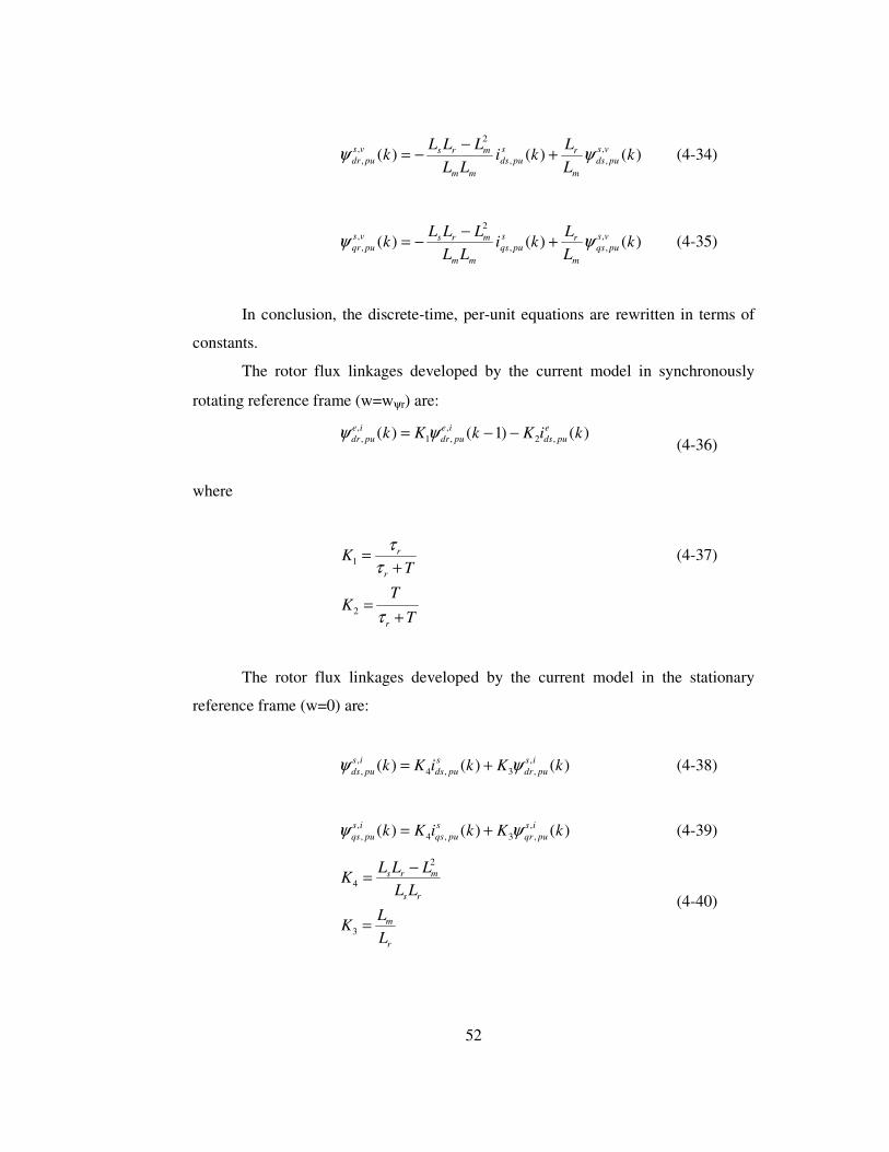
52
)()()( ,,,
2,, k
LL
kiLL
LLLk vs
pudsm
rspuds
mm
mrsvspudr ψψ +−−= (4-34)
)()()( ,,,
2,, k
LL
kiLL
LLLk vs
puqsm
rspuqs
mm
mrsvspuqr ψψ +−−= (4-35)
In conclusion, the discrete-time, per-unit equations are rewritten in terms of
constants.
The rotor flux linkages developed by the current model in synchronously
rotating reference frame (w=wψr) are:
)()1()( ,2
,,1
,, kiKkKk e
pudsie
pudrie
pudr −−= ψψ (4-36)
where
T
TK
TK
r
r
r
+=
+=
τ
ττ
2
1 (4-37)
The rotor flux linkages developed by the current model in the stationary
reference frame (w=0) are:
)()()( ,,3,4
,, kKkiKk is
pudrs
pudsis
puds ψψ += (4-38)
)()()( ,,3,4
,, kKkiKk is
puqrs
puqsis
puqs ψψ += (4-39)
r
m
rs
mrs
LL
K
LLLLL
K
=
−=
3
2
4
(4-40)

53
The back emf’s developed by the voltage model in the stationary reference
frame (w=0) is
)()()()( ,,,5,, kukiKkuke spudscomp
spuds
spuds
spuds −−= (4-41)
)()()()( ,,,5,, kukiKkuke spuqscomp
spuqs
spuqs
spuqs −−= (4-42)
b
sb
VRI
K =5 (4-43)
The stator flux linkages developed by the voltage model in the stationary
reference frame (w=0) are:
)2
)1()(()1()( ,,
6,,
,,
−++−=
kekeKkk
spuds
spudsvs
pudsvs
puds ψψ (4-44)
)2
)1()(()1()( ,,
6,,
,,
−++−=
kekeKkk
spuqs
spuqsvs
puqsvs
puqs ψψ (4-45)
bm
b
IL
TVK =6 (4-46)
The rotor flux linkages developed by the voltage model in the stationary
reference frame (w=0) are:
)()()( ,,7,8
,, kKkiKk vs
pudss
pudsvs
pudr ψψ +−= (4-47)
m
r
mm
mrs
LL
K
LLLLL
K
=
−=
7
2
8
(4-48)
The rotor flux angle developed by the voltage model

54
��
���
�= −
)()(
tan21
)(,
,
,,
1, k
kk
pudrvs
puqrvs
pur ψψ
πθψ (4-49)
The rotor flux angle is computed by referring to a look-up table of 0°-45°
entries. The required parameters for this module are summarized as follows:
• The machine Parameters:
• Stator resistance (Rs)
• Rotor resistance (Rr)
• Stator leakage inductance (Lsl)
• Rotor leakage inductance (Lrl)
• Magnetizing inductance (Lm)
• The based quantities:
• Base current (Ib)
• Base phase voltage (Vb)
• The sampling period
• Sampling period (T)
The stator self inductance is Ls=Lsl+Lm and the rotor self inductance is
Lr=Lrl+Lm.
4.2 Speed Estimation
In this section a speed observer for the 3-phase induction motor based upon
its mathematical model is investigated. The estimator’s accuracy relies heavily on
knowledge of critical motor parameters. The open loop speed estimator employed in
this FOC structure is a well-known method based on stationary reference frame. The
structure of this algorithm is quite easy when compared to the advanced estimation
techniques. The synchronous speed, we, can be easily calculated from the derivative
of the rotor flux angle in (4-10).

55
)
tan 1
dt
d
dt
dsdr
sqr
er
���
�
�
�
��
�
�
�
==
−
ψψ
θω ψ (4-50)
Note that (4-50) can be solved as
dtdu
udtud
+=
−
11)(tan 1
(4-51)
where sdr
sqru
ψψ
= . The solution is then
����
�
�
����
�
�−
== 22
2
)()()(
sdr
sdrs
qr
sqrs
dr
sr
sdrr
edt
ddt
d
dt
d
ψ
ψψψ
ψ
ψψθ
ω ψ (4-52)
Substituting (4-1) and (4-2) into (4-52), and a suitable rearrangement of them gives
the synchronous speed, we as;
[ ]sds
sqr
sqs
sdr
r
msr
rr
e iiL
dt
dψψ
τψω
θω ψ −+== 2)(
1 (4-53)
The second term of the right hand in (4-53) is known as slip that is
proportional to the electromagnetic torque when the rotor flux magnitude is
maintaining constant. The electromagnetic torque can be shown here as;
[ ]sds
sqr
sqs
sdr
r
me ii
LLp
T ψψ −=22
3 (4-54)
where p is the number of poles. Thus, the rotor speed can be found as
[ ]sds
sqr
sqs
sdr
r
msr
er iiL
ww ψψτψ
−−= 2)(1
(4-55)

56
4.2.2 Speed Estimation in Discrete Time and Per-Unit
If the per-unit concept setforth here is applied to (4-55), then, the equation
becomes
���
�
���
� −−= 2
,
,,,,,, )(
1s
pur
spuds
spuqr
spuqs
spudr
rbpuepur
ii
www
ψψψ
τ (4-56)
where wb=2πfb is the base electrical angular velocity (rad/sec), ψb=LmIb is the base
flux linkage (volt.sec), and Ib is the base current (amp). Equivalently, another form
for (4-56) is
���
�
���
� −−= 2
,
,,,,1,, )( s
pur
spuds
spuqr
spuqs
spudr
puepur
iiKww
ψψψ
(4-57)
where rbw
Kτ1
1 = .
The per-unit synchronous speed can be calculated as
dt
dw
fdt
d
fw purpur
puebb
pue,,
,,1
21 ψψ θθπ
== (4-58)
where fb is the base electrical (supply) frequency (Hz) and 2π is the base angle (rad).
Discretizing (4-58) by using backward approximation, yields
���
�
� −−=
T
kdkd
fkw purpur
bpue
)1()(1)( ,,
,ψψ θθ
(4-59)
where T being the sampling period (sec). Equivalently, another form for (4-59) is
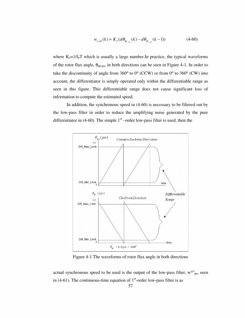
57
))1()(()(,,2, −−= kdkdKkwpurpurpue ψψ θθ (4-60)
where K2=1/fbT which is usually a large number.In practice, the typical waveforms
of the rotor flux angle, θψr,pu, in both directions can be seen in Figure 4-1. In order to
take the discontinuity of angle from 360° to 0° (CCW) or from 0° to 360° (CW) into
account, the differentiator is simply operated only within the differentiable range as
seen in this figure. This differentiable range does not cause significant loss of
information to compute the estimated speed.
In addition, the synchronous speed in (4-60) is necessary to be filtered out by
the low-pass filter in order to reduce the amplifying noise generated by the pure
differentiator in (4-60). The simple 1st –order low-pass filter is used, then the
Figure 4-1 The waveforms of rotor flux angle in both directions
actual synchronous speed to be used is the output of the low-pass filter, w*epu, seen
in (4-61). The continuous-time equation of 1st-order low-pass filter is as

58
)(1 *
,,
*,
puepuec
pue wwdt
dw−=
τ (4-61)
where Tc=1/2πfc is the low-pass filter time-constant (sec), and fc is the cut-off
frequency (Hz). Using backward approximation, then (4-61) becomes
)()1()( ,4*,3
*, kwKkwKkw puepuepue +−= (4-62)
where K3=τc/(τc+T), and K4=T/(τc+T).
As a result, only three equations (4-57), (4-60), and (4-62) are mainly
employed to compute the estimated speed in per-unit. The required parameters for
this method are summarized as follows:
• The machine parameters
• Number of poles (p)
• Rotor resistance (Rr)
• Rotor leakage resistance (Lr1)
• Magneting inductance (Lm)
• The based quantities
• Base current (Ib)
• Base electrically angular velocity (wb)
• The samling period (T)
• Low-pass filter
• Cut-off frequency
• Notice that the rotor self inductance is Lr1+Lm (H)

59
•
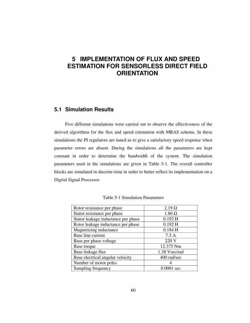
60
5 IMPLEMENTATION OF FLUX AND SPEED ESTIMATION FOR SENSORLESS DIRECT FIELD
ORIENTATION
5.1 Simulation Results
Five different simulations were carried out to observe the effectiveness of the
derived algorithms for the flux and speed estimation with MRAS scheme. In these
simulations the PI regulators are tuned as to give a satisfactory speed response when
parameter errors are absent. During the simulations all the parameters are kept
constant in order to determine the bandwidth of the system. The simulation
parameters used in the simulations are given in Table 5-1. The overall controller
blocks are simulated in discrete-time in order to better reflect its implementation on a
Digital Signal Processor.
Table 5-1 Simulation Parameters
Rotor resistance per phase 2.19 � Stator resistance per phase 1.80 � Stator leakage inductance per phase 0.192 H Rotor leakage inductance per phase 0.192 H Magnetizing inductance 0.184 H Base line current 7.5 A Base per phase voltage 220 V Base torque 12.375 Nm Base linkage flux 1.38 Vsec/rad Base electrical angular velocity 400 rad/sec Number of motor poles 4 Sampling frequency 0.0001 sec

61
5.1.1 Simulation 1- For No-Load Case
During this simulation the motor is rotated at no-load. The electrical speed
command is increased to 0.4 pu that is equal to 1528 rpm (wbase = 400 rad/sec) from
at rest. The reference rotating frame current component (ied) is set to 0.6pu. The aim
of this simulation is to understand the speed estimation accuracy when the torque
command is zero. The Figure 5-1 shows the motor actual torque beside the
commanded torque. In the first 0.1 sec the motor produces electromechanical torque
nearly 1% of rated torque due to motor inertia. After that produced torque settles to
its demanded value and is close to zero.
Figure 5-1 Motor torque at no-load
In
Figure 5-2 rotating frame currents, which are namely torque producing current
component (ieq) and constant flux producing current component (ie
d), are seen. As
seen in the figure qe-axis current component is proportional to the torque produced
while the motor is accelerating. For constant flux operation, de-axis current remains
constant as expected and therefore torque has no oscillations.

62
Figure 5-2 Motor currents (Id, Iq) in rotating reference frame at no-load
The angle of rotor flux with respect to the stationary frame ds-axis is estimated
with the proposed flux observer. In the estimation process as a first step rotor flux
linkages in rotating reference frame are found then the rotor flux angle estimation
follows the calculation method given in section 4.1.1.1. Figure 5-3 shows the rotor
flux angle in pu. One pu here means 2π rad/sec. Note on the graph that the time
elapsed from zero angle to 1.0 pu angle is 0.041 sec. This valuable information gives
us the synchronous speed. Because it says that rotor flux rotates at this speed with
respect to the stationary ds-axis. By this knowledge the rotating reference frame
current components (for example ied and ie
q) can easily be transformed to stationary
reference frame components (for example isd and is
q) or vice versa.
Figure 5-3 Estimated rotor flux angle at no-load

63
When the rotor flux angle is estimated once, synchronous speed and rotor speed can
easily be calculated as given in section 4.2. Figure 5-4 shows the estimated and
actual speed response of the system in the simulation against the set speed value. As
it is seen here MRAS estimates the speed very close to the actual motor speed. The
speed command in this simulation is 0.4 pu which corresponds to 160 rad/sec and
1528 rpm. The actual and estimated motor speeds are measured as 0.415 pu, 0.407
pu, respectively. This means that the speed error accuracy is less than 2.5%. Since
there is no mechanical loading, there does not exist load disturbances and speed
response is therefore quite smooth in time. In this simulation it can be seen that the
settling time for the motor speed is nearly 1.4 seconds. The settling time may change
for different systems according to system performance requirements. For sensorless
algorithms and wide speed ranges it is acceptable in this study.
Figure 5-4 Speed command, motor estimated and actual speeds at no-load

64
Figure 5-5 Currents (is
d and isq) in stationary reference frame at no-load
Motor three-phase currents are transformed to two phase equivalents in
orthogonal system in the machine model and they are shown in Figure 5-5. One can
see from the figure frequency of the stationary frame currents (isd and is
q) are the
same as the rotor flux angle frequency. The amplitudes of the currents are equal to
square root of the sum of squared values of ied and ieq. Since the current ie
q is equal to
zero and the ied is equal to 0.6 pu, the magnitude of the resultant current vector is also
0.6 pu. The phase angle between isd and is
q is 90° as expected.
5.1.2 Simulation 2-For 0.5pu Loading In this simulation the set speed value is the same as the first simulation (i.e. 0.4 pu.),
but a step load torque of 0.5 pu is applied to the shaft of the motor 0.05 seconds later
the simulation starts. The aim of this simulation is to see the motor performance
when a mechanical torque is applied. At the beginning of the simulation, as in
simulation 1, there is an electromechanical torque produced by the motor due to
inertia of the motor. When the motor torque produced decays to zero, a load torque
of 0.5 pu (Base Torque=12,375Nm) is applied to the shaft of the motor as a
command. In Figure 5-6 it is shown that the motor torque settles to its stable point in
0.4 seconds following the loading and makes an overshoot of 1%, which is usually
acceptable for many systems.
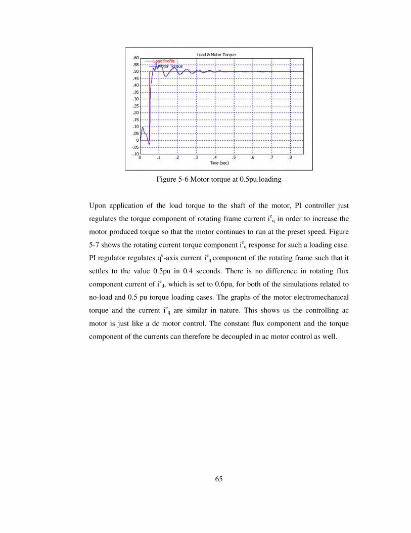
65
Figure 5-6 Motor torque at 0.5pu.loading
Upon application of the load torque to the shaft of the motor, PI controller just
regulates the torque component of rotating frame current ieq in order to increase the
motor produced torque so that the motor continues to run at the preset speed. Figure
5-7 shows the rotating current torque component ieq response for such a loading case.
PI regulator regulates qe-axis current ieq component of the rotating frame such that it
settles to the value 0.5pu in 0.4 seconds. There is no difference in rotating flux
component current of ied, which is set to 0.6pu, for both of the simulations related to
no-load and 0.5 pu torque loading cases. The graphs of the motor electromechanical
torque and the current ieq are similar in nature. This shows us the controlling ac
motor is just like a dc motor control. The constant flux component and the torque
component of the currents can therefore be decoupled in ac motor control as well.
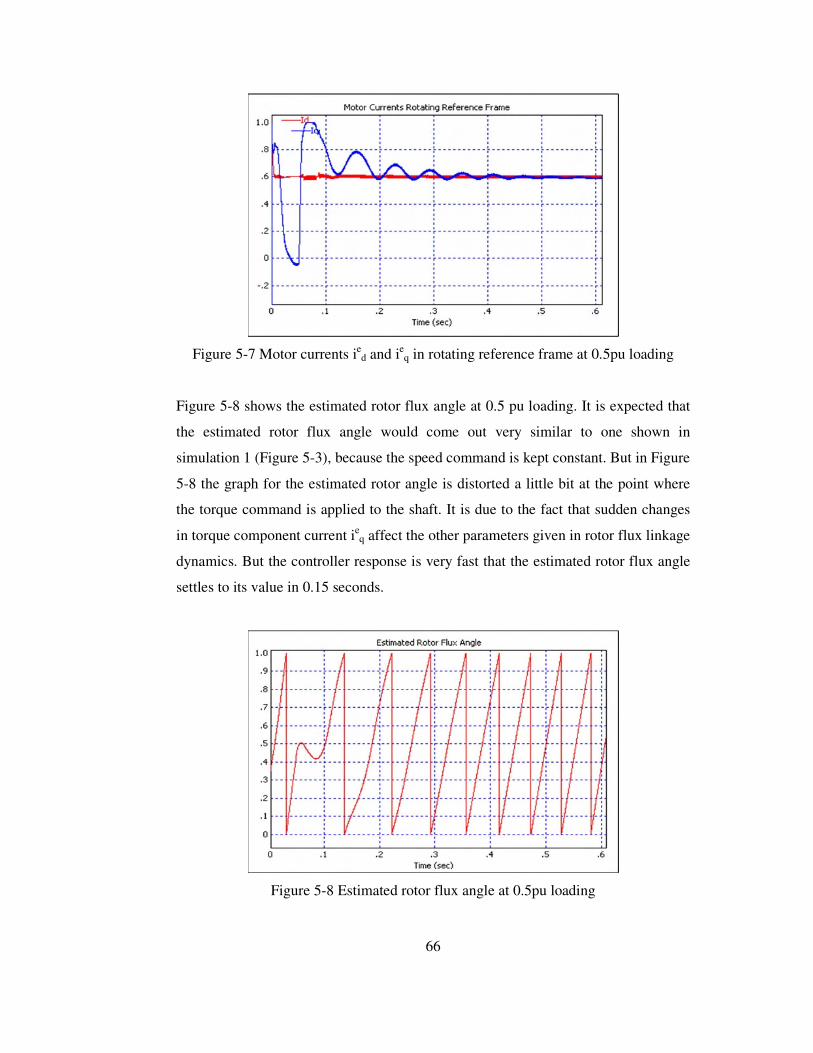
66
Figure 5-7 Motor currents ied and ieq in rotating reference frame at 0.5pu loading
Figure 5-8 shows the estimated rotor flux angle at 0.5 pu loading. It is expected that
the estimated rotor flux angle would come out very similar to one shown in
simulation 1 (Figure 5-3), because the speed command is kept constant. But in Figure
5-8 the graph for the estimated rotor angle is distorted a little bit at the point where
the torque command is applied to the shaft. It is due to the fact that sudden changes
in torque component current ieq affect the other parameters given in rotor flux linkage
dynamics. But the controller response is very fast that the estimated rotor flux angle
settles to its value in 0.15 seconds.
Figure 5-8 Estimated rotor flux angle at 0.5pu loading

67
Speed command, estimated and actual speeds are all shown in Figure 5-9. The
settling time to the desired value for the motor speed increased with respect to that
obtained in simulation 1 (Figure 5-4) due to applied torque. Due to the decrease in
net torque needed for the acceleration, it takes more time for the motor to arrive at
the same speed, as expected. To the contrary of difference resulting in the
acceleration time, the error between the estimated and the actual speeds is the same
with those came out in simulation 1.
Figure 5-9 Speed command, motor estimated and actual speeds at 0.5pu. loading
5.1.3 Simulation 3-For 0.2pu and 0.3 pu Loading
In this simulation the set speed is also 0.4 pu. Torque command is increased
from 0 to 0.2 pu. 0.5 seconds later from the instant of departure from the rest.
Another 0.5 seconds later the torque command is further increased by 0.3 pu again.
Thus, the torque command reached to a total value of 0.5 pu at the end. In this
simulation rotating frame flux component current ied is kept also constant. This
simulation is done for understanding the controller and the motor behaviour when the
torque command is increased in steps. The durations taken while accelerating to the
desired speed value are investigated. Figure 5-10 shows the electromagnetic torque
produced by the motor and the torque demand from it. Up to 0.5 sec the response of
the motor is the same as that obtained in the first simulation (Figure 5-1). The motor

68
responds immediately to setting the torque to 0.2 pu and sets its developed torque to
0.2 pu in return. It complies to another step rise of the torque applied 0.5 seconds
later as well.
Figure 5-10 Motor torque at 0, 0.2 and 0.3 pu. loading
When a torque command is applied to the motor, it is expected that controller
responds this demand by increasing the rotating frame torque component current ieq
in proportion. The expected value for the flux component current ied is the same as
the previous value (0.6pu). The graphs of these currents are shown in Figure5-11.
The value of the torque component current ieq following the application of both
torque commands is equal to the one obtained in simulation 2 (Figure 5-7). This is an
expected behaviour. The only but a minor difference noted in the figure is
oscillations in ieq. These are transients left from the operation of the system prior to
the application of the first torque command. The motor has not reached by then to
steady-state yet, and it was still trying to overcome the effect of motor inertia.

69
Figure 5-11 Motor currents ie
d and ieq in rotating reference frame at 0.2 and 0.3 pu loading
As expected the rotor flux angle has not changed because, the speed command is
being kept constant as previous. There are minor distortions at the points where the
torque is being applied, but it does not affect over all system response and is skipped
here.
Figure 5-12 Estimated rotor flux angle at 0.2 and 0.3pu loading
From the estimated rotor flux angle the speed is estimated and shown together with
the actual motor speed in Figure 5-13. At the point where the 0.2 pu torque is applied
the actual and the estimated speeds deviate from the set point by approximately 15%,
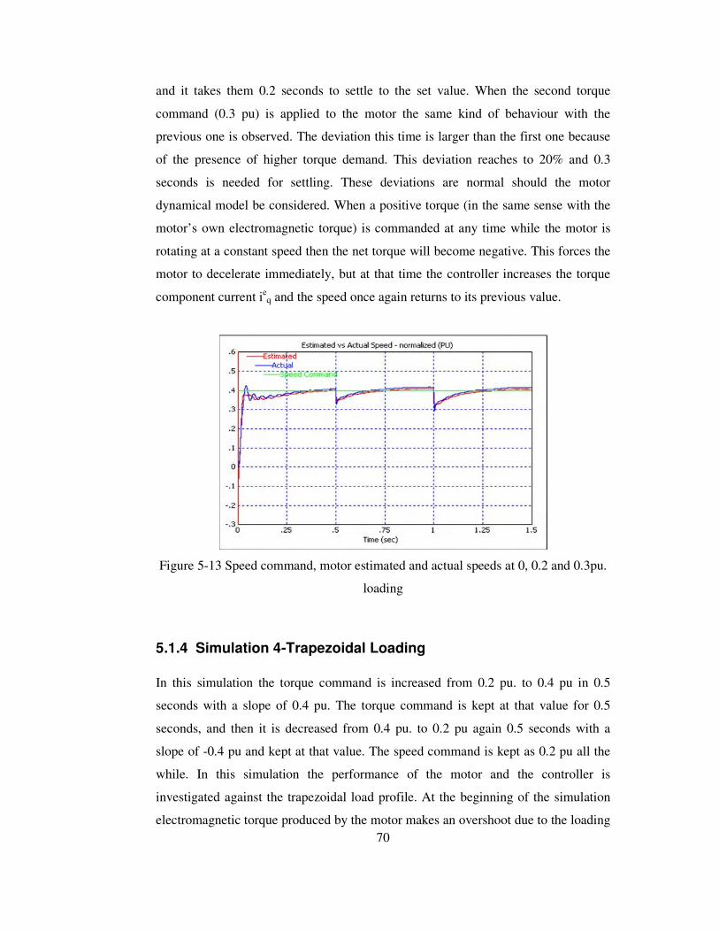
70
and it takes them 0.2 seconds to settle to the set value. When the second torque
command (0.3 pu) is applied to the motor the same kind of behaviour with the
previous one is observed. The deviation this time is larger than the first one because
of the presence of higher torque demand. This deviation reaches to 20% and 0.3
seconds is needed for settling. These deviations are normal should the motor
dynamical model be considered. When a positive torque (in the same sense with the
motor’s own electromagnetic torque) is commanded at any time while the motor is
rotating at a constant speed then the net torque will become negative. This forces the
motor to decelerate immediately, but at that time the controller increases the torque
component current ieq and the speed once again returns to its previous value.
Figure 5-13 Speed command, motor estimated and actual speeds at 0, 0.2 and 0.3pu.
loading
5.1.4 Simulation 4-Trapezoidal Loading In this simulation the torque command is increased from 0.2 pu. to 0.4 pu in 0.5
seconds with a slope of 0.4 pu. The torque command is kept at that value for 0.5
seconds, and then it is decreased from 0.4 pu. to 0.2 pu again 0.5 seconds with a
slope of -0.4 pu and kept at that value. The speed command is kept as 0.2 pu all the
while. In this simulation the performance of the motor and the controller is
investigated against the trapezoidal load profile. At the beginning of the simulation
electromagnetic torque produced by the motor makes an overshoot due to the loading
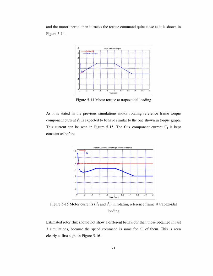
71
and the motor inertia, then it tracks the torque command quite close as it is shown in
Figure 5-14.
Figure 5-14 Motor torque at trapezoidal loading
As it is stated in the previous simulations motor rotating reference frame torque
component current ieq is expected to behave similar to the one shown in torque graph.
This current can be seen in Figure 5-15. The flux component current ied is kept
constant as before.
Figure 5-15 Motor currents (ied and ie
q) in rotating reference frame at trapezoidal
loading
Estimated rotor flux should not show a different behaviour than those obtained in last
3 simulations, because the speed command is same for all of them. This is seen
clearly at first sight in Figure 5-16.
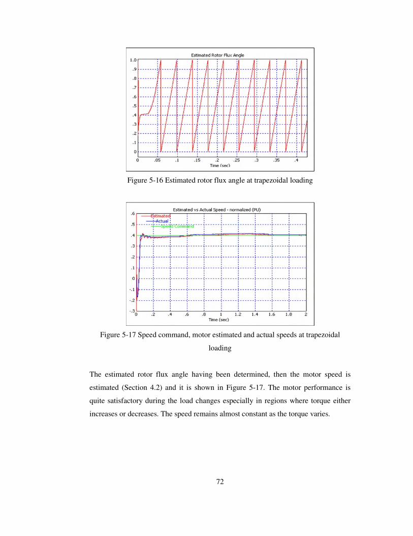
72
Figure 5-16 Estimated rotor flux angle at trapezoidal loading
Figure 5-17 Speed command, motor estimated and actual speeds at trapezoidal
loading
The estimated rotor flux angle having been determined, then the motor speed is
estimated (Section 4.2) and it is shown in Figure 5-17. The motor performance is
quite satisfactory during the load changes especially in regions where torque either
increases or decreases. The speed remains almost constant as the torque varies.
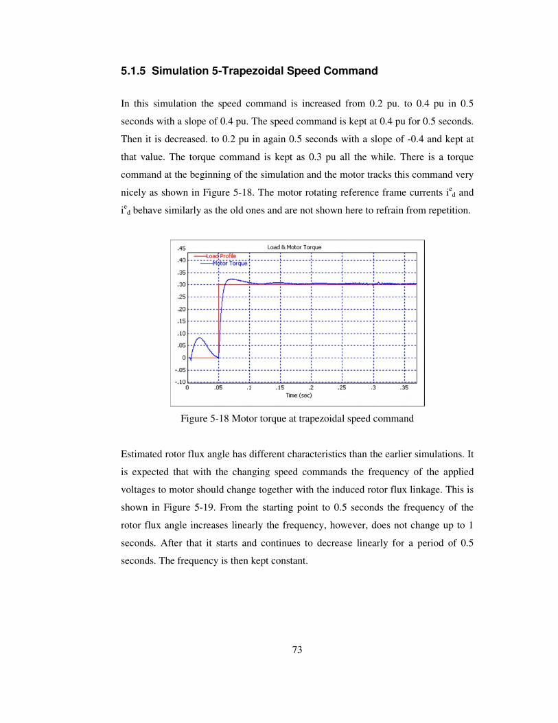
73
5.1.5 Simulation 5-Trapezoidal Speed Command
In this simulation the speed command is increased from 0.2 pu. to 0.4 pu in 0.5
seconds with a slope of 0.4 pu. The speed command is kept at 0.4 pu for 0.5 seconds.
Then it is decreased. to 0.2 pu in again 0.5 seconds with a slope of -0.4 and kept at
that value. The torque command is kept as 0.3 pu all the while. There is a torque
command at the beginning of the simulation and the motor tracks this command very
nicely as shown in Figure 5-18. The motor rotating reference frame currents ied and
ied behave similarly as the old ones and are not shown here to refrain from repetition.
Figure 5-18 Motor torque at trapezoidal speed command
Estimated rotor flux angle has different characteristics than the earlier simulations. It
is expected that with the changing speed commands the frequency of the applied
voltages to motor should change together with the induced rotor flux linkage. This is
shown in Figure 5-19. From the starting point to 0.5 seconds the frequency of the
rotor flux angle increases linearly the frequency, however, does not change up to 1
seconds. After that it starts and continues to decrease linearly for a period of 0.5
seconds. The frequency is then kept constant.

74
Figure 5-19 Estimated rotor flux angle at trapezoidal speed command
Once the rotor flux angle is estimated it is easy to estimate the speed. The set speed,
the actual motor speed, and the estimated speed are altogether shown in Figure 5-20.
Note that, the envelope of the motor actual speed and the estimated speed follow the
speed command, the performance of the controller is not good. This is obviously due
to the poorly selected PI parameters. In case the PI parameters and the constant flux
component of rotating frame current ied are still re-tuned for the case, the response of
the motor speed can be improved. These parameters, however, are kept constant for
all simulations and therefore such a tuning has not been done here in order not to
change bases of comparison for the system behaviours under different loading
conditions. The important point here we are after is the accuracy level achieved for
the speed estimation. We note that the speed estimation error is less than 2%. The
parameters can be re-tuned according to different system requirements.
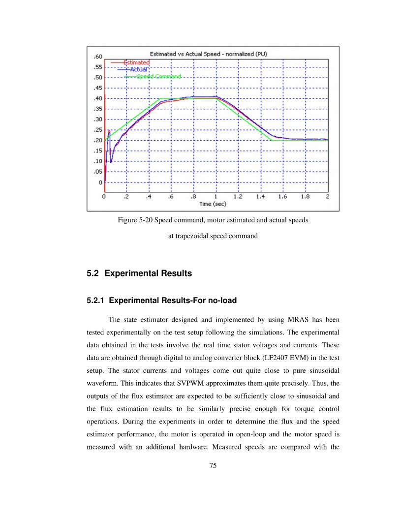
75
Figure 5-20 Speed command, motor estimated and actual speeds
at trapezoidal speed command
5.2 Experimental Results
5.2.1 Experimental Results-For no-load
The state estimator designed and implemented by using MRAS has been
tested experimentally on the test setup following the simulations. The experimental
data obtained in the tests involve the real time stator voltages and currents. These
data are obtained through digital to analog converter block (LF2407 EVM) in the test
setup. The stator currents and voltages come out quite close to pure sinusoidal
waveform. This indicates that SVPWM approximates them quite precisely. Thus, the
outputs of the flux estimator are expected to be sufficiently close to sinusoidal and
the flux estimation results to be similarly precise enough for torque control
operations. During the experiments in order to determine the flux and the speed
estimator performance, the motor is operated in open-loop and the motor speed is
measured with an additional hardware. Measured speeds are compared with the

76
estimated ones. Tests proved that the estimated speed and the supply frequency are
linearly related. Estimated rotor flux angle is used in DSP algorithm for determining
the speed. Estimated rotor flux angle is shown by the DAC of DSP evaluation board.
The line currents together with the stationary axis currents isd and isq are also
investigated during the tests.
The motor is first run at 10Hz and the estimated and actual rotor flux angles
are recorded together. Trace 1(estimated) and trace 2 (actual) shown in Figure 5-21
represent the rotor flux angles with reference to the stator ds-axis position. They
change from 0 to 1pu (2π) as seen in the figure. The time taken for the rotor angle
from zero to 1 shows the full period for the synchronous frequency as 100 msec. The
figure shows clearly the close similarity between the estimated rotor flux angle and
the actual angle. The line current recorded in the test as trace 4 is close to sinusoidal
in shape at 10Hz.
The motor is next run at 20Hz. The results are shown in Figure 5-22. Note on
the figure that trace 1(estimated rotor flux angle) is almost the same as trace 2 (actual
rotor flux angle) indicating that the rotor flux angle is estimated correctly. The
frequencies of both graphs are 20Hz as seen. The line current shown as trace 4 is
close to sinusoidal in shape.

77
Figure 5-21 Ch1 Estimated rotor flux angle, ch2 actual rotor flux angle, ch4 line
current at 10Hz supply frequency
Figure 5-22 Ch1 Estimated rotor flux angle, ch2 actual rotor flux angle, ch4 line
current at 20Hz supply frequency
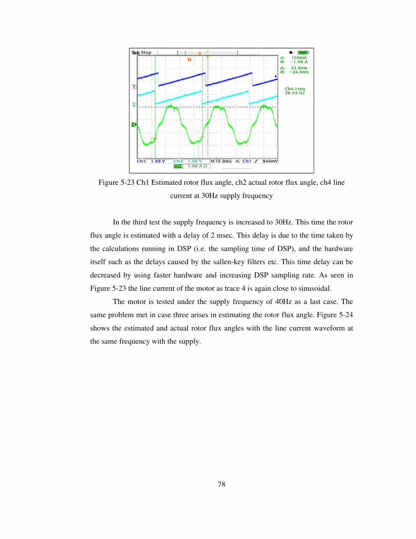
78
Figure 5-23 Ch1 Estimated rotor flux angle, ch2 actual rotor flux angle, ch4 line
current at 30Hz supply frequency
In the third test the supply frequency is increased to 30Hz. This time the rotor
flux angle is estimated with a delay of 2 msec. This delay is due to the time taken by
the calculations running in DSP (i.e. the sampling time of DSP), and the hardware
itself such as the delays caused by the sallen-key filters etc. This time delay can be
decreased by using faster hardware and increasing DSP sampling rate. As seen in
Figure 5-23 the line current of the motor as trace 4 is again close to sinusoidal.
The motor is tested under the supply frequency of 40Hz as a last case. The
same problem met in case three arises in estimating the rotor flux angle. Figure 5-24
shows the estimated and actual rotor flux angles with the line current waveform at
the same frequency with the supply.
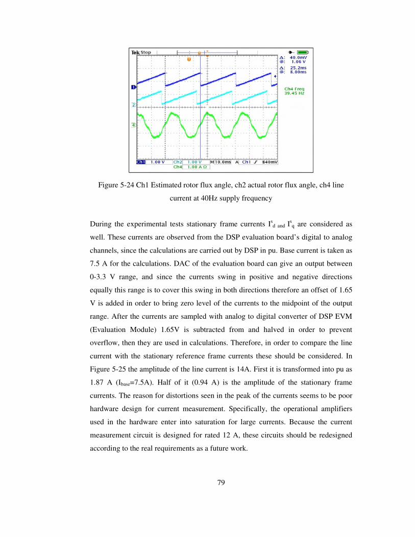
79
Figure 5-24 Ch1 Estimated rotor flux angle, ch2 actual rotor flux angle, ch4 line
current at 40Hz supply frequency
During the experimental tests stationary frame currents Is
d and Isq are considered as
well. These currents are observed from the DSP evaluation board’s digital to analog
channels, since the calculations are carried out by DSP in pu. Base current is taken as
7.5 A for the calculations. DAC of the evaluation board can give an output between
0-3.3 V range, and since the currents swing in positive and negative directions
equally this range is to cover this swing in both directions therefore an offset of 1.65
V is added in order to bring zero level of the currents to the midpoint of the output
range. After the currents are sampled with analog to digital converter of DSP EVM
(Evaluation Module) 1.65V is subtracted from and halved in order to prevent
overflow, then they are used in calculations. Therefore, in order to compare the line
current with the stationary reference frame currents these should be considered. In
Figure 5-25 the amplitude of the line current is 14A. First it is transformed into pu as
1.87 A (Ibase=7.5A). Half of it (0.94 A) is the amplitude of the stationary frame
currents. The reason for distortions seen in the peak of the currents seems to be poor
hardware design for current measurement. Specifically, the operational amplifiers
used in the hardware enter into saturation for large currents. Because the current
measurement circuit is designed for rated 12 A, these circuits should be redesigned
according to the real requirements as a future work.
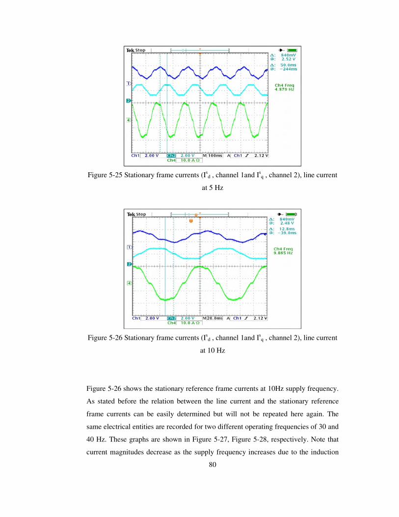
80
Figure 5-25 Stationary frame currents (Is
d , channel 1and Isq , channel 2), line current
at 5 Hz
Figure 5-26 Stationary frame currents (Is
d , channel 1and Isq , channel 2), line current
at 10 Hz
Figure 5-26 shows the stationary reference frame currents at 10Hz supply frequency.
As stated before the relation between the line current and the stationary reference
frame currents can be easily determined but will not be repeated here again. The
same electrical entities are recorded for two different operating frequencies of 30 and
40 Hz. These graphs are shown in Figure 5-27, Figure 5-28, respectively. Note that
current magnitudes decrease as the supply frequency increases due to the induction

81
motor dynamics. At low frequencies back emf of the motor decreases and therefore
the line current increases. Throughout all tests currents come out close to sinusoidal
in shape. This is important for true estimation of rotor flux angle and the speed.
Figure 5-27 Stationary frame currents (Is
d , channel 1and Isq , channel 2), line the
current at 30Hz
Figure 5-28 Stationary frame currents (Isd , channel 1and Is
q , channel 2), line current
at 40Hz
Table 5-2 shows the estimated speeds measured through the digital to analog
converter channels of EVM at 5, 10, 15, 20, 25, 30, 35, 40, 45, and 50 Hz supply
frequencies with an offset of 1.5 V. For each supply frequency expected speeds

82
(rad/sec) are calculated first. Then their pu representations are shown. If the offset is
subtracted from the measured estimated speeds it is obviously seen that the expected
values are similar to estimated ones. The linearity between the estimated speeds and
the supply frequency can easily be seen in Figure 5-29. There are some points where
the linearity is lost, but this may be due to measurement error made in noisy
environment. Also there may be some errors when these data are interpolated.
Table 5-2 Estimated speeds (pu) for different supply frequencies
f(Hz) Speed (rad/sec) Speed (pu) Base speed=400rad/sec
Estimated Speed (pu) with an offset 1.5
50 157 0,39 1,88 45 141,3 0,35 1,84 40 125,6 0,31 1,81 35 109,9 0,27 1,77 30 94,2 0,24 1,74 25 78,5 0,20 1,71 20 62,8 0,16 1,67 15 47,1 0,12 1,64 10 31,4 0,08 1,61 5 15,7 0,04 1,55

83
Supply Frequency (Hz) vs Estimated Speed (pu)
00,050,1
0,150,2
0,250,3
0,350,4
0 10 20 30 40 50 60
freq (Hz)
Est
imat
ed S
peed
(pu)
Figure 5-29 Estimated speed versus supply frequency
5.2.2 Experimental Results- For 0.1pu torque loading
The state estimator designed and implemented by using MRAS has been tested
experimentally on the test setup when 0.1 pu load is applied. For this purpose a dc
machine is coupled to the motor and used in generator mode. An electronic load,
which draws a constant current of 10 A continuously, is connected to the armature
terminals of the dc generator. For different speeds the voltages at the terminals of the
dc machine are measured. From the voltages and currents and known value of the
armature resistance the power dissipated on the dc machine is calculated by using
well-known dc machine model. By considering the efficiency of dc machine, the
mechanical power applied at the shaft of the dc machine, identically the mechanical
power output from the induction machine, is determined. This power is divided by
the measured speed in rad/sec then the torque developed by the induction motor is
calculated. Theoretically dc machine electromechanical torque is dependent on the
armature current when the field mmf is kept constant. For that reason in order to
keep the torque applied to the motor shaft at different speeds, the load current is kept
constant also.
The ac motor is operated in open-loop at different speeds, by applying 10, 20,
30, 40, 50 Hz supply frequencies with the applied torque. The actual and the
estimated rotor flux angles and one of the line current of the motor are recorded. The

84
stationary reference frame currents isd and isq have pure sinusoidal waveforms but
they are not shown here. The exact results of the estimated the rotor flux angle prove
that these currents are pure sinusoidal.
The motor is first run at 10Hz. In Figure 5-30 estimated rotor flux angle is
shown together with the actual one. Trace 1(actual) and trace 2 (estimated) represent
the rotor flux angles with reference to the stator ds-axis position. They change from 0
to 1 pu (2π) as seen in the figure. The time elapsed from zero value of the rotor angle
to 1 show the full period for the synchronous frequency as 100 msec. The figure
shows clearly the close similarity between the estimated rotor flux angle and the
actual angle. The line current recorded in the test as trace 4 is close to sinusoidal in
shape at 10Hz.
Figure 5-30 Ch1 actual rotor flux angle, ch2 estimated rotor flux angle, ch4 line
current at 10Hz supply frequency for 0.1 pu loading
The motor is next run at 20Hz. The results are shown in Figure 5-31. Note that
trace 1(estimated rotor flux angle) is almost the same as trace 2 (actual rotor flux
angle) indicating that the rotor flux angle is estimated correctly. The frequencies in
both graphs are 20 Hz as seen. The line current shown in Figure 5-31 as trace 4 is
close to sinusoidal in shape.

85
Figure 5-31 Ch1 actual rotor flux angle, ch2 estimated rotor flux angle, ch4 line
current at 20Hz supply frequency for 0.1 pu loading
After that the supply frequency is increased to 30Hz. This time the rotor flux angle is
estimated with a delay of 2 msec because of the same reason defined for the no-load
operation at 30 Hz before. As seen in Figure 5-32 the line current of the motor as
trace 4 is again close to sinusoidal.
Figure 5-32 Ch1 actual rotor flux angle, ch2 estimated rotor flux angle, ch4 line
current at 30Hz supply frequency for 0.1 pu loading
Figure 5-33 shows the estimated and actual rotor flux angles with the line current
waveform at the same frequency with the supply.
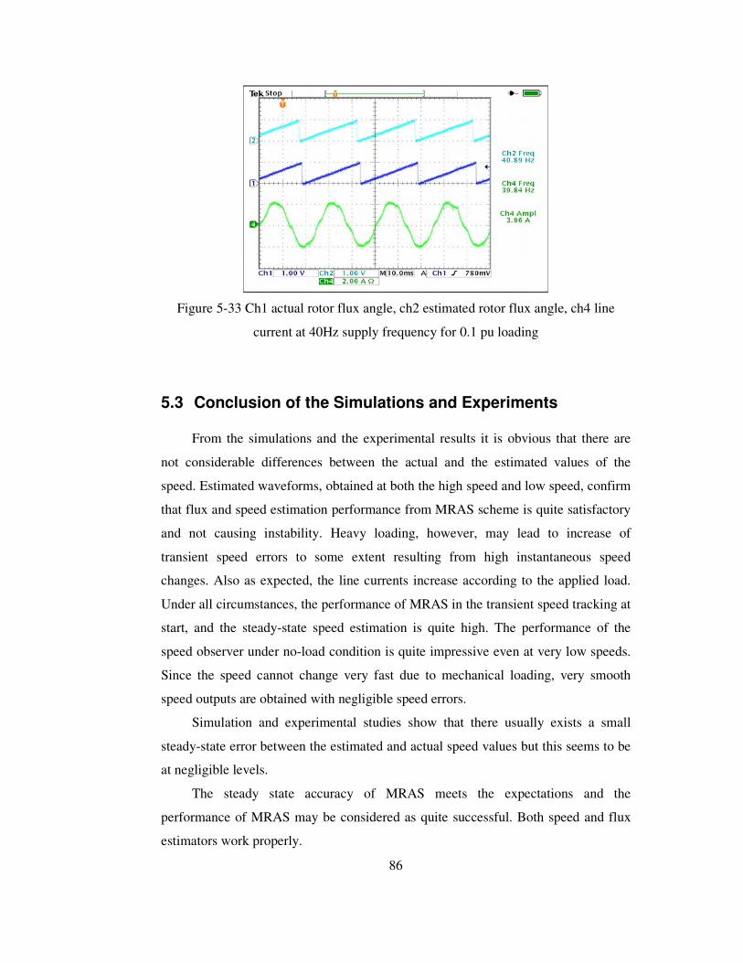
86
Figure 5-33 Ch1 actual rotor flux angle, ch2 estimated rotor flux angle, ch4 line
current at 40Hz supply frequency for 0.1 pu loading
5.3 Conclusion of the Simulations and Experiments
From the simulations and the experimental results it is obvious that there are
not considerable differences between the actual and the estimated values of the
speed. Estimated waveforms, obtained at both the high speed and low speed, confirm
that flux and speed estimation performance from MRAS scheme is quite satisfactory
and not causing instability. Heavy loading, however, may lead to increase of
transient speed errors to some extent resulting from high instantaneous speed
changes. Also as expected, the line currents increase according to the applied load.
Under all circumstances, the performance of MRAS in the transient speed tracking at
start, and the steady-state speed estimation is quite high. The performance of the
speed observer under no-load condition is quite impressive even at very low speeds.
Since the speed cannot change very fast due to mechanical loading, very smooth
speed outputs are obtained with negligible speed errors.
Simulation and experimental studies show that there usually exists a small
steady-state error between the estimated and actual speed values but this seems to be
at negligible levels.
The steady state accuracy of MRAS meets the expectations and the
performance of MRAS may be considered as quite successful. Both speed and flux
estimators work properly.

87
6 THE HARDWARE & SOFTWARE
In this chapter, the hardware configuration of experimental setup and the
software organization is summarized. The hardware configuration of the project is
basically the combination of an asynchronous motor, a motor drive and a
microprocessor. The software of the project involves assembly code of the FOC and
state observers in modular strategy.
6.1 The Motor The experimental setup of this thesis is as shown in Figure 6-1. While testing
the setup, different motor sizes are used, but in the actual experimental stage 3kW
squirrel cage induction motor (Siemens make) is used. In order to obtain motor
parameters, classical no-load and locked-rotor tests are carried out on the motor. For
the initial guess to the parameters used in the FOC algorithm is obtained from the
steady-state equivalent model of the induction motor shown in Figure 6-1. In the real
time applications, motor drives are expected to derive motor parameters during the
initialization of the system by means of properly injected signals and then estimate
on-line by the FOC algorithm embedded in the system during normal running. These
methods are skipped in this work and considered as future work. In this thesis,
different from on-line parameter estimation, closed-loop observer (e.g. MRAS) is
expected to compensate the effects of parameter deviations regarding the parameter
errors as system noise. Referring to the equivalent circuit of the machine in Figure
6-2.

88

89
Figure 6-2 Approximate per phase equivalent circuit for an induction machine
Rs is obtained by dc-test, Rc and Xm are determined by no-load and the rest of the
parameters are determined by locked-rotor test. The stator resistance of each stator
winding can be measured independently by applying a dc-current to one phase as
shown in Figure 6-3.
Figure 6-3 Diagram of dc measurement
The stator resistance is measured on the motor terminals by applying a current
through a resistor and measuring the corresponding voltage, or without a resistor
applying low-level dc voltage. To obtain a more accurate measurement result, one
must get several numbers of measured data and take the average of these data for
each phase.
The leakage-reactances xls, xlr and the rotor resistance are determined when
the motor speed is set to zero, i.e. s=1. Since the magnetizing branch elements are
large enough compared to the rest of the equivalent components, these are neglected
in this test. It is further assumed that leakage reactances are equal to each other
according to IEEE test standards. Since stator resistance is measured and leakage

90
reactances are assumed to be equal, rotor resistance can easily be calculated from the
measured data. The measurements are done around the rated current of the motor and
than the average of the measurements are computed to obtain more approximate
parameters.
When the motor is running without load, the slip will be close to zero. Thus,
the variable slip resistance will be very large. Therefore, in the no-load test one may
consider the magnetizing branch as the approximate circuit of the motor model. The
no-load data are measured around the rated voltage, and magnetizing branch
elements are calculated around the rated voltage of the motor. The calculated motor
parameters and ratings of the motor are given in Table 6-1.
Table 6-1 Motor Parameters per phase
Rs (stator resistance) 1.8� Rr ( referred rotor resistance) 2.18� Rc 522 ohm Xm (magnetizing reactance) 63.7� Xls,Xlr (leakage reactances) 2,69� Ls,Lr (stator & rotor induc.) 0,192H Lls,Llr (leakage induc.) 0,00084H Lm (magnetizing induc.) 0,184H
6.2 The Motor Drive The drive circuit used here has been developed in another work but modified
to suit to the requirements of this work [25]. The drive mainly includes a rectifier, dc-
link circuit and an inverter. The rectifier used in this drive is Semikron-SKD28 that
consists of six uncontrolled diodes. The rated output current of the rectifier is 28 A
and the rated operating voltage is 1300 V. During the tests, the three-phase voltage is
supplied over an autotransformer to the rectifier.
In the dc-link circuit, the rectified voltage is a smooth dc filtered by two dc-
link capacitors each being 1000µF and connected in series. In addition to them a
resistor of 30K�, 1W, is connected across each capacitor to equalize their voltage
sharing. The dc link voltage is impressed on the capacitors through a relay system as
shown in the Figure 6-4.
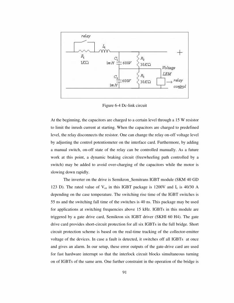
91
Figure 6-4 Dc-link circuit
At the beginning, the capacitors are charged to a certain level through a 15 W resistor
to limit the inrush current at starting. When the capacitors are charged to predefined
level, the relay disconnects the resistor. One can change the relay on-off voltage level
by adjusting the control potentiometer on the interface card. Furthermore, by adding
a manual switch, on-off state of the relay can be controlled manually. As a future
work at this point, a dynamic braking circuit (freewheeling path controlled by a
switch) may be added to avoid over-charging of the capacitors while the motor is
slowing down rapidly.
The inverter on the drive is Semikron_Semitrans IGBT module (SKM 40 GD
123 D). The rated value of Vce in this IGBT package is 1200V and Ic is 40/30 A
depending on the case temperature. The switching rise time of the IGBT switches is
55 ns and the switching fall time of the switches is 40 ns. This package may be used
for applications at switching frequencies above 15 kHz. IGBTs in this module are
triggered by a gate drive card, Semikron six IGBT driver (SKHI 60 H4). The gate
drive card provides short-circuit protection for all six IGBTs in the full bridge. Short
circuit protection scheme is based on the real-time tracking of the collector-emitter
voltage of the devices. In case a fault is detected, it switches off all IGBTs at once
and gives an alarm. In our setup, these error outputs of the gate-drive card are used
for fast hardware interrupt so that the interlock circuit blocks simultaneous turning
on of IGBTs of the same arm. One further constraint in the operation of the bridge is

92
that no IGBT is turned on unless the gate charge of the other IGBT is completely
removed.
The output of the inverter is connected to the motor through current sensors
to acquire information about currents in real-time. Overall diagram of the inverter is
shown in Figure 6-5.
Figure 6-5 Inverter circuit
6.3 The DSP
In order to run the real-time control algorithm and create PWM signals, Texas
Instruments’ (TI) TMS320 processor is used in this work. Texas Instruments’
TMS320 family consists of fixed-point, floating-point, multiprocessor digital signal
processors (DSPs). TMS320 DSPs have an architecture designed specifically for
real-time signal processing. The LF2407 is a member of the “C2000 DSP” platform,
and is optimized specifically for control applications. The “C24x series” of DSP
controllers combine this real-time processing capability with controller peripherals to
create a suitable solution for vast majority of control system applications. The
following characteristics make the TMS320 family a suitable choice for a wide range
of processing applications:
• Flexible instruction set,
• Inherent operational flexibility,

93
• High-speed performance,
• Innovative parallel architecture,
• Cost effectiveness.
TMS320F2407 version of this family is the one used in this application. It uses a 16-
bit word length along with 32-bit registers for storing intermediate results, and has
two hardware shifters available to scale numbers independent of the CPU.
The C24x DSP controllers take advantage of an existing set of peripheral
functions which includes:
• Timers,
• Serial communications ports (SCI, SPI),
• Analog-to-digital converters (ADC),
• Event manager,
• System protection, such as low-voltage detection and watchdog timers.
To function as a system manager, a DSP must have robust on-chip I/O and
other peripherals. The event manager of the LF2407 is application-optimized
peripheral unit, coupled with the high-performance DSP core, enables the use of
advanced control techniques for high-precision and high-efficiency full variable-
speed control of motors. Included in the event manager are special pulse-width
modulation (PWM) generation functions, such as a programmable dead-band
function and a space-vector PWM state machine for 3-phase motors that provides
quite a high efficiency in the switching of power transistors. Three independent
up/down timers, each with it’s own compare register, support the generation of
asymmetric (non-centered) as well as symmetric (centered) PWM waveforms.
6.4 Interface Card
In order to convey information back and forth between the power stage and
DSP an interface card has been designed. Moreover, suitable signal amplification,
signal filtering and hardware protection properties are added to this interface card
(see Appendix A).
The dc-link voltage is sensed with a voltage sensor (LV25_P) on the interface
card. The insulation property of the voltage sensor is quite sufficient to protect the

94
digital circuit and low voltage analog circuit from high voltage part. The magnitude
of the dc-link voltage is sensed to re-build the phase voltages (Vsd & Vs
q) in the
control software with the information of duty-cycles of the IGBTs (Appendix B).
Another aim of the voltage sensor is to sense the overcharge on the dc-link
capacitors. If the voltage level exceeds the predefined limit that is determined by the
user, a comparator gives an error signal. This error signal is used for immediate
hardware interrupt and all the IGBTs are set to off-state. Finally, to take the power
resistance used in the dc link line to limit the in-rush current at starting out, the dc
link voltage level information is needed to operate the relay across this resistance.
The voltage sensor also provides this voltage information whether it exceeds the
adjusted voltage level or not. If this mechanism is employed then the relay will
operate automatically after the start command in a very short time.
In addition, the PWM signals generated by DSP are amplified to make them
compatible with the gate drive card inputs. For this purpose, six PWM signals are
adjusted to 15V individually without any other change. Finally, all the errors, gate
drive card errors, over-voltage error, over-current error, and an external error are OR
gated. The single error output from this gate is assigned to control PWM-OFF circuit
to set the all IGBTs to off-state in case of any fault. Figure 6-6 shows the DSP
interface card.

95
Figure 6-6 Dsp interface card
6.5 Current Interface Card
The other sensed variables are stator currents using current-sensor on the
interface card. For this purpose LA 25-NP current transducers are used. These
sensors are capable of sensing AC, DC and mixed current waveforms. The sensor has
multi-range current sensing options depending on the pin connections. The sensors
use hall-effect phenomena to sense the current. They have excellent accuracy and
very good linearity in the operating range. The output of these sensors is between
±15V and unipolar. Since the ADCs on the DSP board cannot sense the negative
voltage and requires signal between 0-3.3V, our current sensors are used with current
interface card. Normally, one must add offset to the AC current signals to
compensate the negative parts and then subtract this amount in the software.
Furthermore, the current signals must be normalized between the 0-3.3V range using
amplifiers before the ADCs. All of these procedures cause extra uncertainty that
affects the accuracy of the sensed information.
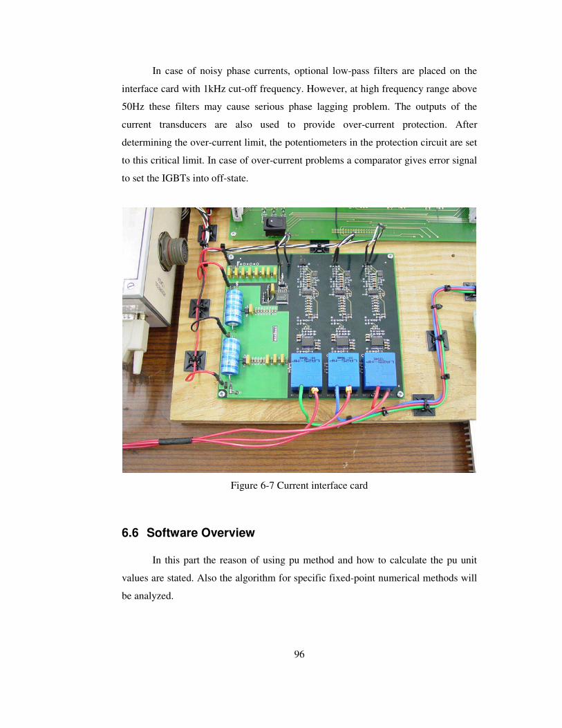
96
In case of noisy phase currents, optional low-pass filters are placed on the
interface card with 1kHz cut-off frequency. However, at high frequency range above
50Hz these filters may cause serious phase lagging problem. The outputs of the
current transducers are also used to provide over-current protection. After
determining the over-current limit, the potentiometers in the protection circuit are set
to this critical limit. In case of over-current problems a comparator gives error signal
to set the IGBTs into off-state.
Figure 6-7 Current interface card
6.6 Software Overview
In this part the reason of using pu method and how to calculate the pu unit
values are stated. Also the algorithm for specific fixed-point numerical methods will
be analyzed.
97
6.6.1 Base Values and PU model
Since the TMS320LF2407 is a fixed point DSP, PU (per unit) model of the
motor is used to increase the accuracy and simplify the overall system. In a fixed
point system, 16 bit words are assigned to variables and some of the bits are used for
integer part of the number and some for floating part. To increase the accuracy, one
must reserve as many bits as possible to floating part. This is also possible with pu
system. If the pu parameters and variables are properly chosen, the integer part will
expected to be at most 1± and the number of the bits reserved for the floating part
will be maximized.
While choosing the pu values, one may select ratings of the motor or multiple
of the nominal values as base depending on the operating conditions. One must be
careful about the transient regions, since the amount of the states may exceed the
unity in transient state. Thus, the multiple of the nominal values may be adjusted
according to the transient state peak values to limit the base values. However, this
will give harm to the accuracy of the steady-state computations. Due to this reason,
while testing the performance of the observers, we run the system under light-load
conditions. The base quantities are calculated as shown below:
(6.1)
where Ib, Vb, are the maximum values of the phase nominal current and voltage; wb
is the electrical nominal rotor flux speed; �b is the base flux and subscript n is
expresses the nominal quantities of the same variable. The real time quantities are
implemented in to the control thanks to the pu quantities, which are defined as
follows:
b
bb
nb
nb
nb
wV
fw
VKV
IKI
=
===
ψ
π2
*
*
1
1

98
b
b
b
VV
v
II
i
ψψψ =
=
=
(6.2)
6.6.2 Fixed-Point Arithmetic
In binary format, a number can be represented in signed magnitude, where the
left-most bit represents the sign and the remaining bits represent the magnitude.
Two’s complement is an alternative form of representation used in most processors,
including the TMS320. The representation of a positive number is the same in two’s
complement and in signed magnitude. Thus the first bit gives idea whether the
number represented in signed magnitude is positive or negative.
In fixed-point operations Qk format is used to represent the floating numbers.
For example, in Q12 format, first bit is assigned for sign and three bits are assigned to
represent the integer part and the rest of the 16 bits is assigned for floating part of the
number. In Q15, one bit is assigned for sign and the rest is assigned for floating part.
Thus one can represent the number in the range of -1 to 1 excluding these to
integers. So if the variables are normalized in a proper way those never exceed unity,
Q15 format provides the best accuracy. If one uses numbers greater than unity then,
the Qk format must be rearranged to represent those numbers. For example, using Q12
format the numbers between the –7.999 to +7.999 with a less accuracy in the floating
part since the floating part may be represented with fewer numbers when compared
to the Q15 format. The resolution of the Q15 format is 0.0000305 (1/215) where Q12
format is 0.000244 (1/212). If the selected base values are in nominal values, than
drive control quantities will not be greater than four times the nominal values (for the
most part). In this case one may use Q12 format. On the other hand, if the value of the
variables are guaranteed to be less than unity by choosing proper base quantities, Q15
format is preferred . The generalized representation of Qk is given below:
k
kk
kk
k bbbbbbZ −−
−−
−−
−−
−− ++++++−= 2*....2*2*......2*2* 2
21
1014
1415
15 (6.3)

99
where k represent the number of bits representing floating part and b is the binary
(0,1) quantities. Here are some examples to clarify the concept:
pi=3.14159265= 0011.0010 0100 0011 in Q12 format (3243H)
= 011.0 0100 1000 0111 in Q13 format (6486H)
0.0045 = 0000. 0000 0001 0010 in Q12 format
= 0.000 0000 1001 0110 in Q15 format
The summation of the numbers in Qk format is the same as binary system
summation. However, the multiplication has some tricks. In the multiplication of the
Qk format, the result is in the form of: Qn*Qm = Qn+m. Since the multiplication
operation is done in the 32 bit accumulator, Qn+m may exceed to Q30 without any
problem.
For example, Q12*Q12 = Q24
Figure 6-8 Multiplication in dsp accumulators
After the multiplication Q24 is stored to the accumulator as shown in accumulator_I
(Figure 6-8). The right bits of the shaded part are neglected in accumulator_I. Before
storing to a 16-bit microprocessor word, the number in the accumulator must be left
shifted as in the case of accumulator_II and than the high word in the accumulator
must be stored the associated word. In the multiplication of Qk format n and m above
may be any number between 0-15. However, 16-bit result must be aligned to either
high or low word of the accumulator in the form of any Q15 format.

100
7 CONCLUSION and FUTURE WORK
7.1 Conclusion
The focus of this thesis has been the Direct Field Control of induction
machine. Modified direct torque and flux control strategy based on two PI controllers
and a voltage space-vector modulator module are used in order to observe rotor flux,
stator flux, synchronous speed and rotor flux angle.
First, generalized dynamic mathematical model of the induction machine is
studied in different reference frames. Induction machine mathematical model in
stationary frame is investigated.
Next, Model reference adaptive system based closed-loop direct torque
control of induction machines is simulated. A flux observer with voltage model-
current model combination is implemented. The outputs of this observer were fed to
an open-loop speed estimator. Also an experimental drive system was build and
tested at high and low speeds using the same technique. It was shown that DTC-
SVM strategy realizes almost ripple-free operation for the entire speed range. The
flux, speed, and torque estimations are improved.
It can be stated that, using the DTC-SVM topology, the overall system
performance is increased.
7.1 Future Work
This simulations and experimental works show the benefits of closed-loop
full-order flux and speed observer models using MRAS technique. Due to
experimental limitations the algorithm could not tested over a wide speed and torque
ranges. In the future this work can be implemented.

101
Other MRAS algorithms based on reactive power regulation may be used for
speed prediction.
Other sensorless techniques can be tested and the advantages and the
disadvantages of the model can be clarified after the tests.
The machine parameters and the rotor time-constant can be estimated and
used in the flux observer module and the closed-loop control can be improved.
102
REFERENCES
[1] B.K.Bose, “Power Electronics and AC Drives”, Prentice Hall, 1986
[2] P.Vas "Sensorless Vector and Direct Torque Control" New York: O.
University Press, (1998)
[3] I.Boldea and S.A.Nasar, “Vector Control of AC Drives”, CRC Press, 1992.
[4] D.W.Novotny and T.A.Lipo, “Vector Control and Dynamics of AC Drives”,
Oxford University Press Inc., Oxford, New York, 1997.
[5] R.D.Doncker and D.W.Novotny “The universal field oriented controller”,
IEEE Tran. IA, vol. 30 no .1, pp. 92-100, January, 1994
[6] R.Lorenz “Tuning of the field oriented induction motor controller for high
performance applications”, IEEE Tran. IA, vol. 22, pp. 293-297, 1986
[7] K.B.Nordinand D.W. Novotny “The influence of motor parameter deviations
in feed forward field oriented drive systems” IEEE Tran. IA, vol. 21,
pp.1009-1015, July 1985
[8] R.Krishman, F.C.Doran “Study of parameter sensitivity in high performance
inverter-fed induction motor drive systems”, IEEE Tran. IA, vol. 23, pp.623-
635, 1987
[9] P.L.Jansen and R.D.Lorenz “Transducer less position and velocity estimation
in induction an salient ac machines”, IEEE Tran. IA, vol. 31, no.2, pp.240-
247, Mar/April, 1995
103
[10] R.Gabriel, W.Leonhard and C.Nordby “ Field oriented control of standard
AC motor using microprocessor”, IEEE Tran. IA, vol.16, no.2, pp.186.192,
1980
[11] H.Jun and W.Bin “New integration Algorithms for Estimating Motor Flux
over a Wide Speed Range” IEEE Tran. IE, vol. 13, no.5, pp.969-977, 1998
[12] P.L.Jansen and R.D.Lorenz “Observer based direct field orientation: Analysis
and comparison of alternative methods”, IEEE Tran. IA, vol. 30, no.4,
pp.945-953, Jul/Aug, 1994
[13] G.C.Vershese and S.R.Sanders “Observers for flux estimation in the
induction machine” IEEE Tran. IE, vol. 35, no.1, pp.85-94, 1998
[14] Lennart Harneffors “Design and analysis of general rotor-flux oriented vector
control system” IEEE Tran. IE, vol. 48, no.2, pp.383-390, 2001
[15] G.Yang and T.Chin “Adaptive-Speed identification scheme for a vector
controlled speed sensorless inverter induction motor drive” ,IEEE Tran. IA,
vol. 29, no.4, pp.820-825, 1993
[16] B.Robyns, B.Frederique, “A methodology to determine gains of induction
motor flux observers based on a theoretical parameter sensitivity analysis”,
IEEE Tran. PE, vol. 15, no.6, pp.983-995, 2000
[17] A.M.Trzynadlowski, “The Field Oriented Principle in Control of induction
Motors”, Kluwer Academic Publisher, Norwell, MA, 1994

104
[18] M.Elbuluk, N.Langovsky and D.Kankam “Design and Implementation of a
Closed Loop Observer and Adaptive Controller for Induction Motor Drives”
IEEE Tran. IA vol. 34 no. 3 pp. 435-443, May/June 1998
[19] H.Tajima, Y.Hori “Speed Sensorless Field Orientation Control of the
Induction Machine” IEEE Tran. IA vol. 29, no. 1, pp. 175-180, Feb.1993
[20] C.Schauder “Adaptive Speed Identification for Vector Control of Induction
Motor without Rotational Transducers” IEEE Tran. IA vol. 28, no. 5, pp.
1054-1061, Oct.1992
[21] F.Z.Peng, T.Fukao “Robust Speed Identification for Speed Sensorless Vector
Control of Induction Motors” IEEE Tran. IA vol. 30, no. 5, pp.1234-1239,
Oct.1994
[22] L.Zhen and L. Xu “Sensorless Field Orientation Control of Induction
Machines Based on Mutual MRAS Scheme” IEEE Tran. IE vol. 45 no. 5, pp.
824-831, October 1998
[23] C.Lascu, I.Boldea, F.Blaabjerg “A Modified Direct Torque Control for
Induction Motor Sensorless Drive” IEEE Tran. IA vol. 36, no. 1, pp. 122-130,
Jan 2000
[24] B. Akın, “State Estimation Techniques for Speed Sensorless Field Oriented
Control of Induction Machines” M.S Thesis EE Dept. Metu Aug. 2003
[25] B. Mutluer, “Vector Control of Asynchronous Motors” M.S Thesis EE Dept.
Metu Dec. 1999
[26] Texas Instruments, “Digital Motor Control Software Library”, Literature
number: SPRU 485A Oct. 2003

105
[27] Texas Instruments, “ACI3-4 3-Phase Induction Motor Control”, App. Note,
15 Nov. 2000
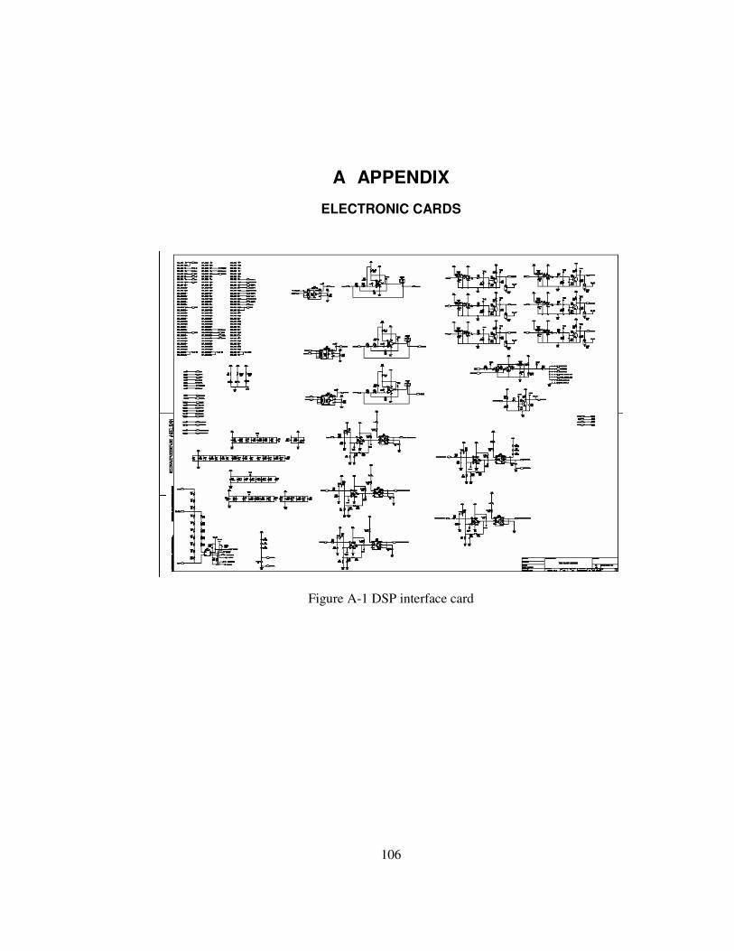
106
A APPENDIX
ELECTRONIC CARDS
Figure A-1 DSP interface card
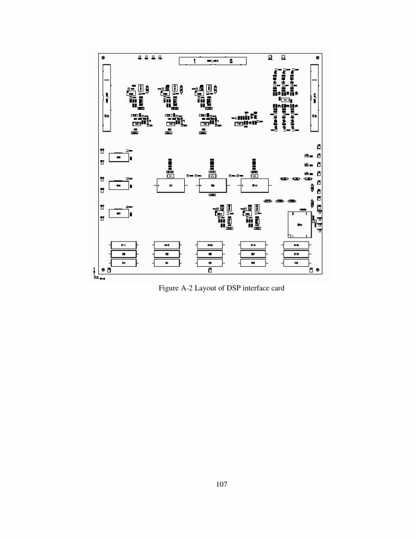
107
Figure A-2 Layout of DSP interface card

108
Figure A-3 View of DSP Interface Card

109
Figure A-4 Current interface card

110
Figure A-5 Layout of current interface card
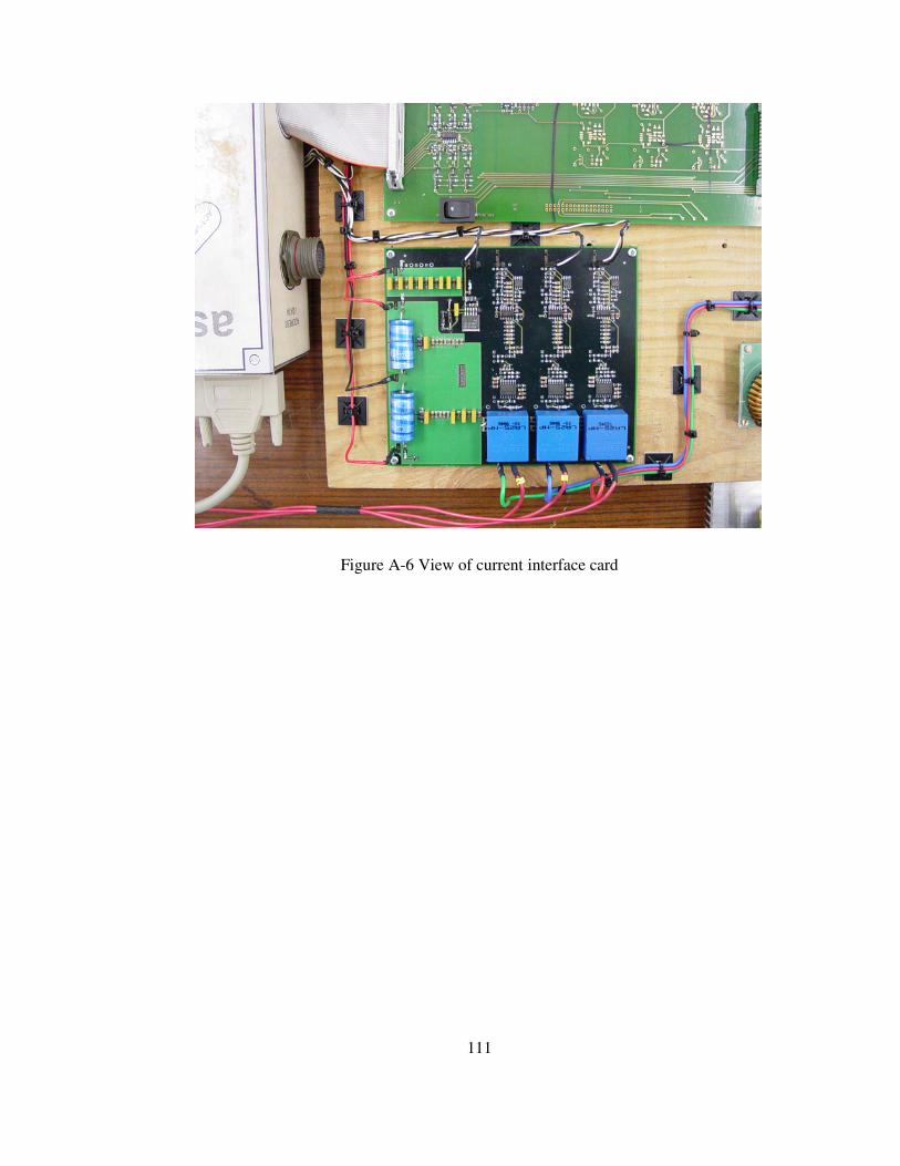
111
Figure A-6 View of current interface card

112
Figure A-7 View of DSP card
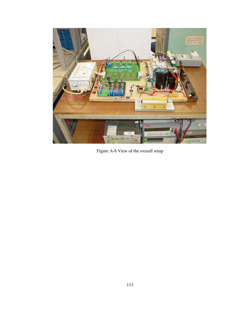
113
Figure A-8 View of the overall setup

114
B APPENDIX
ACQUISITION of the STATOR VOLTAGES
The induced voltage, which is the signal to be integrated for flux vector
estimation, is obtained as the difference between the stator voltage and the resistive
voltage drop across the machine windings. When a voltage source inverter (VSI) is
used to feed the machine, the stator voltages are formed by pulse trains having a
typical rise time 2-10kV/µs. These are digitally acquired at a high, though limiting
sampling rate. The limited bandwith of such sampling process may fail to establish
the exact volt-second equivalent between the actual and the acquired signals, and
hence produce an error. To avoid this complication, some people use current source
inverter or a linear power amplifier.
To avoid this problem in a switched VSI drive, it is preferred to replace the
actual stator voltages by the reference voltage vector that controls the pulsewidth
modulator.
The phase voltage of a general 3-phaase motor (Van, Vbn, Vcn) can be
calculated from the DC-bus voltage (Vdc), and three upper switching functions of
inverter (S1, S2, and S3). The 3-ph windings of motor are connected either ∆ or Y
without a neutral return path (or 3-ph, 3-wire system). The overall system is shown
in Figure 2.
Each phase of the motor is simply modeled as a series impedance of
resistance and inductance (r, L) and back emf (ea, eb, ec). Thus, three phase voltages
can be computed as

115
aa
anaan edtdi
LriVVV ++=−= (B-1)
bb
bnbbn edtdi
LriVVV ++=−= (B-2)
cc
cnccn edtdi
LriVVV ++=−= (B-3)
Summing these three phase voltages, yields
cbacba
cbancba eeedt
iiidLriiiVVVV ++++++++=−++ )(
)(3 (B-4)
For a 3-phase system with no neutral path and balanced back emfs,
ia+ib+ic=0, and ea+eb+ec,=0. Therefore, equation,
cbacba
cbancba eeedt
iiidLriiiVVVV ++++++++=−++ )(
)(3 (B-4 (B-5)
becomes, Van+Vbn+Vcn,=0. Furthermore, the neutral voltage can be simply derived
from (B-5) as
)(31
cban VVVV ++= (B-6)
Now three phase voltages can be calculated as
cbacbaaan VVVVVVVV31
31
32
)(31 −−=++−= (B-7)
cabcbabbn VVVVVVVV31
31
32
)(31 −−=++−= (B-8)
baccbaccn VVVVVVVV31
31
32
)(31 −−=++−= (B-9)
Three voltages Va, Vb, Vc are related to the DC-bus voltage (Vdc) and three
upper switching functions (S1, S2, S3) as:
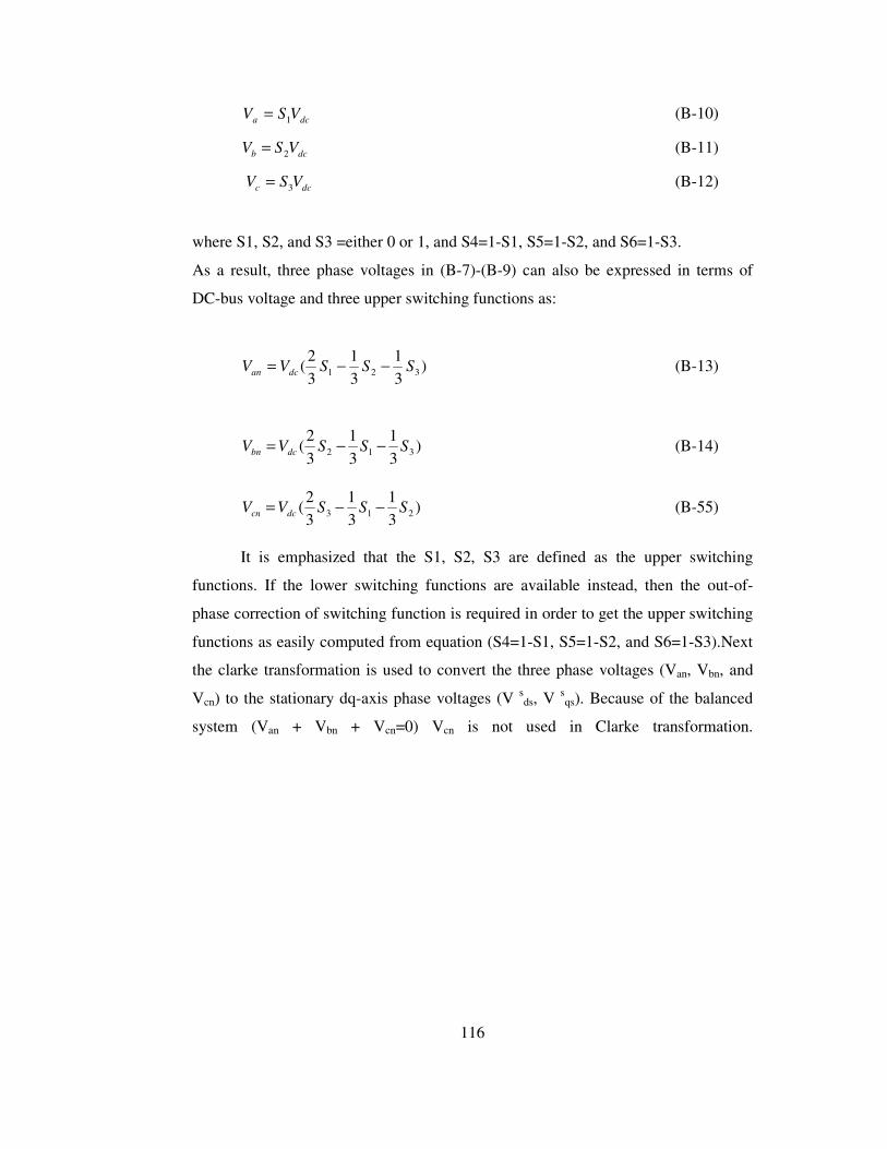
116
dca VSV 1= (B-10)
dcb VSV 2= (B-11)
dcc VSV 3= (B-12)
where S1, S2, and S3 =either 0 or 1, and S4=1-S1, S5=1-S2, and S6=1-S3.
As a result, three phase voltages in (B-7)-(B-9) can also be expressed in terms of
DC-bus voltage and three upper switching functions as:
)31
31
32
( 321 SSSVV dcan −−= (B-13)
)31
31
32
( 312 SSSVV dcbn −−= (B-14)
)31
31
32
( 213 SSSVV dccn −−= (B-55)
It is emphasized that the S1, S2, S3 are defined as the upper switching
functions. If the lower switching functions are available instead, then the out-of-
phase correction of switching function is required in order to get the upper switching
functions as easily computed from equation (S4=1-S1, S5=1-S2, and S6=1-S3).Next
the clarke transformation is used to convert the three phase voltages (Van, Vbn, and
Vcn) to the stationary dq-axis phase voltages (V sds, V s
qs). Because of the balanced
system (Van + Vbn + Vcn=0) Vcn is not used in Clarke transformation.
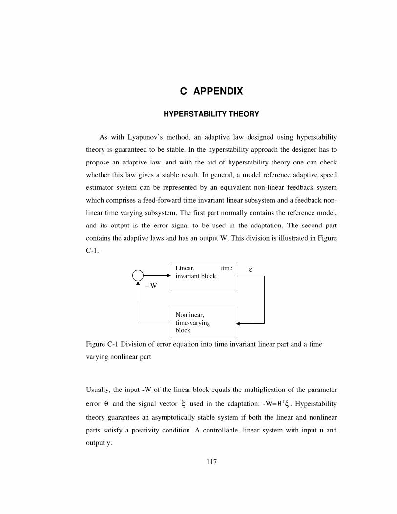
117
Linear, time invariant block
Nonlinear, time-varying block
W−
ε
C APPENDIX
HYPERSTABILITY THEORY
As with Lyapunov’s method, an adaptive law designed using hyperstability
theory is guaranteed to be stable. In the hyperstability approach the designer has to
propose an adaptive law, and with the aid of hyperstability theory one can check
whether this law gives a stable result. In general, a model reference adaptive speed
estimator system can be represented by an equivalent non-linear feedback system
which comprises a feed-forward time invariant linear subsystem and a feedback non-
linear time varying subsystem. The first part normally contains the reference model,
and its output is the error signal to be used in the adaptation. The second part
contains the adaptive laws and has an output W. This division is illustrated in Figure
C-1.
Usually, the input -W of the linear block equals the multiplication of the parameter
error θ and the signal vector ξ used in the adaptation: -W= ξθT . Hyperstability
theory guarantees an asymptotically stable system if both the linear and nonlinear
parts satisfy a positivity condition. A controllable, linear system with input u and
output y:
Figure C-1 Division of error equation into time invariant linear part and a time
varying nonlinear part

118
is said to be positive real (PR) if Re[H(s)] equal or greater than zero. Hence the real
part of the transfer function can never become negative as long as the real part of s is
larger than or equal to zero. According to hyperstability theory the linear part H must
be strictly positive real (SPR) which means that the real part of H(jw) is larger than
zero for all W>0 thus Nyquist diagram of H(jw) must lie in the right half of the
complex plane, including the imaginary axis. This implies that the number of poles
and zeros in H(s) differs at most by 1, and the phase shift is never larger than 90o.
The nonlinear part must satisfy Popov’s integral inequality, which states that a
positive constant 20γ exists such that:
This requirement is also denoted the passivity requirement. Observing nonlinear part
as an electrical network, the inequality can be shown to state that the amount of
energy output by the nonlinear system is never larger than the sum of the incoming
energy and the energy stored in the system. The energy in the system depends on the
external input of power and on the power generation in the system
dtd
[stored energy]=[ext. power input] + [int. power generation]
Considering ε , the input, as voltage and W as output, current, the external power
input equals ε W. If the internal power generation is negative, the system is said to
B)AsI(C)s(U)s(Y
)s(H
:functiontransferawith
xCy
BuAxx
1T
T
−−==
=+=�
0tallfordtW 1
t
0
20
1
≥γ−≥•ε

119
be dissipative or strictly passive. If the internal power generation is less than or equal
to zero, the system is passive. Strict passivity is equivalent to SPR and asymptotic
stability. The main result using positivity and passivity concepts is that any parallel
combination of passive blocks is also passive. A feedback combination of two
passive blocks in which at least one is strictly passive. This is of great interest in
hyperstability theory, in which an SPR (and hence strictly passive) linear block is
connected to a passive nonlinear block in a feed back configuration. This
combination is strictly passive (and hence asymptotically stable).