sensor simulation based hyperspectral image …

SENSOR SIMULATION BASED HYPERSPECTRAL IMAGE ENHANCEMENT WITHMINIMAL SPECTRAL DISTORTION

A. Khandelwala, ∗, K. S. Rajanb

a Dept. of Computer Science and Engineering, University of Minnesota, 200 Union Street SE, Minneapolis, USA - [email protected] Lab for Spatial Informatics, International Institute of Information Technology, Gachibowli, Hyderabad 500032, India - [email protected]

KEY WORDS: Hyperspectral Image Fusion, Spectral Response Functions, Spectral Distortion, Sensor Simulation, Vector Decompo-sition

ABSTRACT:

In the recent past, remotely sensed data with high spectral resolution has been made available and has been explored for various agri-cultural and geological applications. While these spectral signatures of the objects of interest provide important clues, the relativelypoor spatial resolution of these hyperspectral images limits their utility and performance. In this context, hyperspectral image enhance-ment using multispectral data has been actively pursued to improve spatial resolution of such imageries and thus enhancing its usefor classification and composition analysis in various applications. But, this also poses a challenge in terms of managing the trade-offbetween improved spatial detail and the distortion of spectral signatures in these fused outcomes. This paper proposes a strategy ofusing vector decomposition, as a model to transfer the spatial detail from relatively higher resolution data, in association with sensorsimulation to generate a fused hyperspectral image while preserving the inter band spectral variability. The results of this approachdemonstrates that the spectral separation between classes has been better captured and thus helped improve classification accuraciesover mixed pixels of the original low resolution hyperspectral data. In addition, the quantitative analysis using a rank-correlation metricshows the appropriateness of the proposed method over the other known approaches with regard to preserving the spectral signatures.

1. INTRODUCTION

Hyperspectral imaging or imaging spectroscopy has gain consid-erable attention in remote sensing community due to its utility invarious scientific domains. It has been successfully used in is-sues related to atmosphere such as water vapour (Schlpfer et al.,1998), cloud properties and aerosols (Gao et al., 2002); issuesrelated to eclogoy such as chlorophyll content (Zarco-Tejada etal., 2001), leaf water content and pigments identification (Chenget al., 2006); issues related to geology such as mineral detec-tion (Hunt, 1977); issues related to commerce such as agriculture(Haboudane et al., 2004) and forest production.

The detailed pixel spectrum available through hyperspectral im-ages provide much more information about a surface than is avail-able in a traditional multispectral pixel spectrum. By exploitingthese fine spectral differences between various natural and man-made materials of interest, hyperspectral data can support im-proved detection and classification capabilities relative to panchro-matic and multispectral remote sensors (Lee, 2004) (Schlerf et al.,2005) (Adam et al., 2010) (Govender et al., 2007) (Xu and Gong,2007).

Though hyperspectral images contain high spectral information,they usually have low spatial resolution due to fundamental trade-off between spatial resolution, spectral resolution, and radiomet-ric sensitivity in the design of electro-optical sensor systems. Thus,generally multispectral data sets have low spectral resolution buthigh spatial resolution. On the other hand, hyperspectral datasetshave low spatial resolution but high spectral resolution. Thiscoarse resolution results in pixels consisting of signals from morethan one material. Such pixels are called mixed pixels. This phe-nomenon reduces accuracy of classification and other tasks (Villaet al., 2011b) (Villa et al., 2011a).

With the advent of numerous new sensors of varying specifica-tions, multi-source data analysis has gained considerable atten-

∗Corresponding author.

tion. In the context of hyperspectral data, Hyperspectral ImageEnhancement using multispectral data has gained considerableattention in the very recent past. Multi-sensor image enhance-ment of hyperspectral data has been viewed with many perspec-tives and thus a variety of approaches have been proposed. Algo-rithms for pansharpening of multispectral data such as CN sharp-ening (Vrabel, 1996), PCA based sharpening (Chavez, 1991),Wavelets based fusion (Amolins et al., 2007) have been extendedfor hyperspectral image enhancement. Component substitutionbased extensions such as PCA based sharpening suffer from thefact that information in the lower components which might becritical in classification and detection may be discarded and re-placed with the inherent bias that exist due to band redundancy.Frequency based methods such as Wavelets have the limitationthat they are computationally more expensive, requires appro-priate values of the parameters and in general does not preservespectral characteristics of small but significant objects in the im-age. Various methods (Gross and Schott, 1998) using linear mix-ing models have been proposed to obtain sub pixel compositionswhich are then distributed spatially under spatial autocorrelationconstraints. The issue with these algorithms is that they do nothave robust ways of determining spatial distribution of pixel com-positions. Recently, methods incorporating Bayesian framework(Eismann and Hardie, 2005) (Zhang et al., 2008) have been pro-posed that model the enhancement process in a generative modeland achieve enhanced image as maximum likelihood estimate ofthe model. The challenge with these methods is that they makevarious assumptions on distribution of data and require certaincorrelations to exist in data for good performance.

A core issue with most of these algorithms is that they do not con-sider the physical characteristics of the detection system i.e eachsensor works in different regions of the electromagnetic spec-trum. Ignoring this fact leads to injection of spectral informationfrom different part of the spectrum which may not belong to thesensor and this leads to modification of spectral signatures in thefused hyperspectral data. This makes the enhanced image inap-

ISPRS Annals of the Photogrammetry, Remote Sensing and Spatial Information Sciences, Volume II-8, 2014ISPRS Technical Commission VIII Symposium, 09 – 12 December 2014, Hyderabad, India

Band Number Spectral Range of List of band numbersof ALI ALI bands (in µm) from HYPERIONBand 3 0.45 - 0.515 11-16Band 4 0.52 - 0.60 18-25Band 5 0.63 - 0.69 28-33Band 6 0.77 - 0.80 42-45Band 9 1.55 - 1.75 141-160

Band 10 2.08 - 2.35 193-219

Table 1: Set of hyperspectral bands corresponding to each multi-spectral band

propriate for image processing tasks such as classification, objectdetection etc.

Here, we propose a new approach, Hyperspectral Image Enhance-ment Using Sensor Simulation and Vector Decomposition (HySSVD)for improving spatial resolution of hyperspectral data using highspatial resolution multi-spectral data. This paper aims at explor-ing how well enhanced images from different algorithms mimicthe true or desired spectral variability in the fused hyperspectralimage. Through various experiments we show that there exits atrade-off between improvement in spatial detail and distortion ofspectral signatures.

2. DATA

Hyperspectral data from HYPERION sensor on board EO-1 space-craft has been used for this study. HYPERION provides a highresolution hyperspectral imager capable of resolving 220 spec-tral bands (from 0.4 to 2.5 micrometers) with a 30-meter spatialresolution and provides detailed spectral mapping across all 220channels with high radiometric accuracy.For multispectral data, ALI (Advanced Land Imager) sensor onboard EO-1 spacecraft has been used. ALI provides Landsat typepanchromatic and multispectral bands. These bands have beendesigned to mimic six Landsat bands with three additional bandscovering 0.433-0.453, 0.845-0.890, and 1.20-1.30 micrometers.Multispectral bands are available at 30-meter spatial resolution.

Since hyperspectral bands have very narrow spectral range (10nm), they are also referred by their center wavelength. Table 1shows spectral range of multispectral bands that mimic six Land-sat bands together with list of hyperspectral bands whose centerwavelength lie in the range of different multispectral bands.

Since, both hyperspectral data and multispectral data are at 30mspatial resolution, hyperspectral data has been down sampled to120m in this work. Hence the ratio of 4:1 between multispectraldata and hyperspectral data has been established. Moreover, inthis setting hyperspectral data at 30m can be used as validationdata against which output of different algorithms can be com-pared. Here, the hyperspectral data at 30m will be referred to asTHS (True Hyperspectral) and hyperspectral data at 120m will bereferred as OHS (Original Hyperspectral) which will be enhancedby the algorithms. Multispectral data at 30m will be referred toas OMS. Figure 1 shows RGB composites of datasets used in thisstudy. The algorithms use OHS with OMS to generate the fusedhyperspectral image (FHS) at 30m. This fused result would becompared with THS for performance analysis. Figure 1(d) is theclass label information for the given area. As we can see, the re-gion contains four major classes namely Corn (green), Soyabean(yellow), Wheat (red) and Sugarbeets (brown) with pixel distri-bution shown in table 2. This image corresponds to an area inMinnesota, USA. The image has been taken on 21st July, 2012.

Class Pixel CountCorn 45708

Soyabean 98291Wheat 46039

Sugarbeets 20904

Table 2: Pixel Count of major classes

(a) (b) (c) (d)

Figure 1: Study Area. (a) True Hyperspectral (THS) image at30m, (b) Original Multispectral (OMS) image at 30m, (c) Origi-nal Hyperspectral (OHS) image at 120m, (d) Ground Truth mapat 30m

The ground truth is available through NASA’s Cropscape website(Han et al., 2012).

In order to properly show the visual quality of various images,magnified view of the part of image enclosed in dotted lines infigure 1(a) will be used. For statistical analysis, the completeimage will be used.

3. PROPOSED APPROACH

The algorithm presented here, HySSVD has three main stages.Figure 2 shows the flowchart of the algorithm. As a preprocessingstep, original low resolution hyperspectral data (OHS) is upscaledto the spatial resolution of original multispectral data (OMS). Theupscaled data will be referred as UHS. In the first stage, simu-lated multispectral (SMS) bands are generated using UHS bandsand Spectral Response Functions (SRF) of OMS bands. In thesecond stage, each SMS band is enhanced using its correspond-ing OMS band to generate fused multispectral (FMS) bands. Inthird stage, Fused Hyperspectral (FHS) bands are computed byinverse transformation using vector decomposition. Followingsubsections explain each stage in detail.

3.1 Generating Simulated Multispectral (SMS) bands

Hyperspectral data has been considered in remote sensing to cross-calibrate a hyperspectral sensor with another hyperspectral or mul-tispectral sensor (Teillet et al., 2001), and to simulate data offuture sensors (Barry et al., 2002). The algorithm exploits sen-sor simulation capabilities of hyperspectral data using spectralresponse function of the sensor to be simulated. Figure 3 showsspectral response function of a multispectral band from ALI sen-sor (blue curve). The spectral response function of a sensor de-fines the probability that a photon of a given wavelength is de-tected by this sensor. As we can see from the response functionof the band, it is non zero for only some wavelengths and itsresponse varies for different wavelengths. The value recorded bythe sensor is proportional to the total incident light that it was able


Center wavelengths of hyperspectral bands

SRF of an original multispectral band

Band Selection

Upscaled Hyperspectral Bands(UHS) at 120m

Sensor Simulation

Simulated Multispectral Band (SMS) at 120m

Original Multispectral Band (OMS) at 30 m

Spatial Detail Transfer

Fused Multispectral Band (FMS) at 30m

Vector Decomposition Based Detail Transfer

Fused Hyperspectral Bands (FHS) at 30m

Figure 2: Flowchart of the Algorithm

1500 1550 1600 1650 1700 1750 18000

0.2

0.4

0.6

0.8

1

Wavelength

SR

F V

alue

Figure 3: Spectral response function of band 9 of ALI

to detect. In other words, all the wavelengths that a sensor is ableto detect contributes to its value. The weight of the contributionof a particular wavelength is determined by the SRF value at thatwavelength. Ideally, to simulate a multispectral band, we needlight from all wavelengths within the SRF of that band. But thislevel of spectral detail is not available in real sensors. Hyperspec-tral sensors are the closest approximation for the data that can beused for simulating a sensor with wide SRF. As mentioned be-fore, SRFs of hyperspectral bands are generally referred by theircenter wavelengths as they are very narrow. Figure 3 shows thesecenter wavelengths as vertical red lines. The hyperspectral bandsthat contribute in simulation of a multispectral band are the oneswhich have their center wavelength within the spectral range ofthe multispectral band. Table 1 shows the set of hyperspectralbands selected for each multispectral band.

Many methods exist for simulating multispectral data with de-sired wide-band SRFs. Most methods synthesize a multispectralband by a weighted sum of hyperspectral bands, and they are dif-ferent in their ways in determining the weighting factors. Somemethods directly convolve the multispectral filter functions to thehyperspectral data (Green and Shimada, 1997), which is equiva-lent to using the values of the multispectral SRF as the weightingfactors. Some have used the integral of the product of the hyper-spectral and multispectral SRFs as the weight (Barry et al., 2002).Few have calculated the weights by finding the least square ap-proximation of a multispectral SRF by a linear combination of thehyperspectral SRFs ( Slawomir Blonksi, Gerald Blonksi, JeffreyBlonksi, Robert Ryan, Greg Terrie, Vicki Zanoni, 2001). Bowels(Bowles et al., 1996) used a spectral binning technique to get syn-thetic image cubes with exponentially decreasing spectral resolu-tion, where the equivalent weighting factors are binary numbers.

The algorithm presented here has adopted the method described

in (Green and Shimada, 1997). Firstly, all OHS bands are up-scaled to the spatial resolution of the given OMS data to get UHS.If m is the number of bands falling in the range of the multispec-tral band k (OMSk), then let ~Wk be the m dimensional weightvector calculated using spectral response function of the multi-spectral band k. For a pixel at location i,j , let ~UHSi,j,k be them dimensional vector containing the intensity values of those mhyperspectral bands corresponding to (OMSk). The simulatedvalue SMSi,j,k for the pixel i,j can be obtained using the follow-ing equation.

SMSi,j,k = ~WTk

~UHSi,j,k (1)

which is the inner product of the two vectors. The vector ~WTk is

computed asW i

k = SRFk(Ci) (2)

where, SRFk is the spectral response function of the multispec-tral band k and Ci is center wavelength of the hyperspectral bandi.

The reason for creating simulated multispectral bands is two-fold.First, since high spatial detail is available at multispectral reso-lution, transferring spatial detail at multispectral level would bemore effective than transferring spatial detail from a multispectralband to a hyperspectral band directly. Second, this will ensurethat the algorithm is not enhancing a hyperspectral band whosespectral information is not part of a multispectral band in ques-tion. The drawback of this approach is that some hyperspectralbands will not be enhanced. But other approaches will also causespectral distortion in these bands as multispectral data does notcontain information about these bands.

3.2 Generating Fused Multispectral Bands

After stage 1, SMS bands are obtained. These bands have spa-tial resolution same as that of OMS bands but have poor detail ascompared to OMS bands because SMS bands are simulated usingupscaled hyperspectral bands. In this step, spatial detail from anOMS band is transferred to its corresponding SMS band. Thisstep can be seen as sharpening of a grayscale image using an-other grayscale image. One relevant concern here can be that whythere is a need to transfer detail and create a fused multispectralband. Since, theoretically an SMS band is just low spatial reso-lution version of its corresponding OMS band, then OMS banditself can be treated as the fused high spatial resolution versionof SMS bands. But in many real situations multispectral data andhyperspectral data can be from different dates. Because of differ-ent atmospheric conditions and other factors, an OMS can not betaken as a direct enhanced version of its SMS band. Hence, weneed methods that can transfer only spatial detail while not dis-torting the spectral properties of the SMS band. Many methodsexist to do this operation. In this paper Smoothing Filter BasedIntensity Modulation (SFIM) algorithm has been adopted (Liu,2000). SFIM can be represented as

FMSi,j,k =SMSi,j,k ∗OMSi,j,k

OMSi,j,k

(3)

where, OMSi,j,k, SMSi,j,k and FMSi,j,k are original mul-tispectral value, simulated multispectral value and fused multi-spectral value respectively at a pixel i,j for the band k. OMSi,j,k

is the mean value calculated by using an averaging filter for aneighborhood equivalent in size to the spatial resolution of thelow-resolution data. Similarly this operation can be applied toenhance each SMS band leading to the calculation of the corre-sponding FMS band.Figure 4 shows results of this step on only the part enclosed in


(a) OMS band5 (b) SMSband5

(c) FMS band5

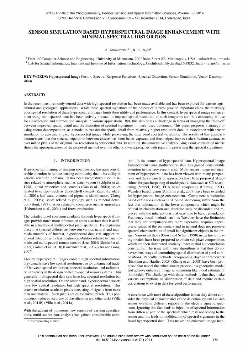
Figure 4: Performance of the Stage 2 spatial detail transfer

dotted lines in figure 1(a) due to space constraints. Figure 4(a)shows band 5 from original multispectral data (OMS5), whileFigure 4(b) shows simulated multispectral band 5 (SMS5) cor-responding to band 5 of ALI data. Figure 4(c) shows the fusedresult for band 5 (FMS5). It is clearly evident that features havebecome sharper in the fused result. Now this detail has to betransferred to each hyperspectral band that contributed in simula-tion of this band.

3.3 Generating Fused Hyperspectral (FHS) Bands Using Vec-tor Decomposition Method

The previous stage generates FMS bands. The spatial detail fromFMS bands has to be transferred into hyperspectral bands. Here,we explain the process of detail transfer at this stage. Expandingequation 1, we have

w1uhs1+w2uhs2+ ...wm−1uhsm−1+wmuhsm = SMSi,j,k

(4)where wi and uhsi are elements of vectors ~Wk and ~UHSi,j,k

respectively. This is an equation of a m dimensional hyperplaneon which we know a point, ~UHSi,j,k. This plane will be referredas PSMS . Also, say normal of this plane is n̂ . Say ~FHSi,j,k

be the m dimensional vector representing fused hyperspectralvalue for the m selected bands of multispectral band k. Fusedmultispectral (FMS) data can alternatively be estimated using thesensor simulation strategy from section (3.1).

w1f1 + w2f2 + ...wm−1fm−1 + wmfm = FMSi,j,k (5)

where wi and fi are elements of vectors ~Wk and ~FHSi,j,k re-spectively. Again this is an equation of an m dimensional hy-perplane on which we wish to estimate the point ~FHSi,j,k. Thisplane will be referred as PFMS . Equations 4 and 5 represent twoparallel hyperplanes which are separated by a distance d equalto the difference between the simulated and fused multispectralvalues at that pixel ( ~FMSi,j,k - ~SMSi,j,k).

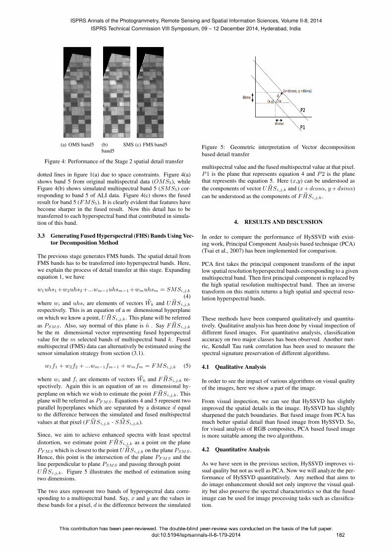
Since, we aim to achieve enhanced spectra with least spectraldistortion, we estimate point ~FHSi,j,k as a point on the planePFMS which is closest to the point ~UHSi,j,k on the planePSMS .Hence, this point is the intersection of the plane PFMS and theline perpendicular to plane PSMS and passing through point~UHSi,j,k. Figure 5 illustrates the method of estimation using

two dimensions.

The two axes represent two bands of hyperspectral data corre-sponding to a multispectral band. Say, x and y are the values inthese bands for a pixel, d is the difference between the simulated

Figure 5: Geometric interpretation of Vector decompositionbased detail transfer

multispectral value and the fused multispectral value at that pixel.P1 is the plane that represents equation 4 and P2 is the planethat represents the equation 5. Here (x,y) can be understood asthe components of vector ~UHSi,j,k and (x+dcosα, y+dsinα)can be understood as the components of ~FHSi,j,k.

4. RESULTS AND DISCUSSION

In order to compare the performance of HySSVD with exist-ing work, Principal Component Analysis based technique (PCA)(Tsai et al., 2007) has been implemented for comparison.

PCA first takes the principal component transform of the inputlow spatial resolution hyperspectral bands corresponding to a givenmultispectral band. Then first principal component is replaced bythe high spatial resolution multispectral band. Then an inversetransform on this matrix returns a high spatial and spectral reso-lution hyperspectral bands.

These methods have been compared qualitatively and quantita-tively. Qualitative analysis has been done by visual inspection ofdifferent fused images. For quantitative analysis, classificationaccuracy on two major classes has been observed. Another met-ric, Kendall Tau rank correlation has been used to measure thespectral signature preservation of different algorithms.

4.1 Qualitative Analysis

In order to see the impact of various algorithms on visual qualityof the images, here we show a part of the image.

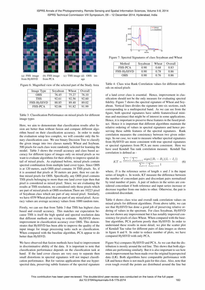
From visual inspection, we can see that HySSVD has slightlyimproved the spatial details in the image. HySSVD has slightlysharpened the patch boundaries. But fused image from PCA hasmuch better spatial detail than fused image from HySSVD. So,for visual analysis of RGB composites, PCA based fused imageis more suitable among the two algorithms.

4.2 Quantitative Analysis

As we have seen in the previous section, HySSVD improves vi-sual quality but not as well as PCA. Now we will analyze the per-formance of HySSVD quantitatively. Any method that aims todo image enhancement should not only improve the visual qual-ity but also preserve the spectral characteristics so that the fusedimage can be used for image processing tasks such as classifica-tion.


(a) FHS imagefrom HySSVD

(b) FHS imagefrom PCA

(c) THS image (d) OHS im-age

Figure 6: Magnified view of the selected part of the Study Area

Image Type Soyabean Wheat OverallOHS 76.45 75.27 76.10THS 92.61 92.56 92.60

FHS-HySSVD 88.85 89.40 89.02FHS-PCA 92.06 91.82 91.99

Table 3: Classification Performance on mixed pixels for differentimage types

Here, we aim to demonstrate that classification results after fu-sion are better than without fusion and compare different algo-rithm based on their classification accuracy. In order to makethe evaluation setup less complex, we will consider only the bi-nary classification case. We use binary Decision Tree to classifythe given image into two classes namely Wheat and Soybean.500 pixels for each class were randomly selected for learning themodel. Table 3 shows the overall accuracy and class based ac-curacy for different types of images only on mixed pixels as wewant to evaluate algorithms for their ability to improve spatial de-tail of mixed pixels. As explained before, mixed pixels containspectral combination from multiple land cover types. Since OHSis at 120 meters, each OHS pixel contains 16 THS pixels. So, ifit is assumed that pixels at 30 meters are pure, then we can de-fine mixed pixels for OHS. Specifically, any OHS pixel containsTHS pixels belonging to more than one land cover type then thatpixel is considered as mixed pixel. Since, we are evaluating theresults at THS resolution, we considered only those pixels whichare part of mixed pixels at OHS resolution.There are 10223 pixelof Soyabean class which are part of any mixed pixel. Similarly,we have 4559 Wheat pixel that are part of any mixed pixel. Accu-racy values are average accuracy values from 1000 random runs.

Firstly, we can see that from Table 3 that THS has highest classbased and overall accuracy. This matches our expectation be-cause THS is itself the high spatial and spectral resolution datathat different methods are trying to estimate. HySSVD showsimprovement in classification accuracy over OHS. This demon-strates that HySSVD has been able to improve the quality of theinput image for image processing tasks such as classification.When compared with the baseline algorithm, PCA appear to dobetter than HySSVD.

We have observed that fusion methods have lead to improvementin discriminative ability of the data. It is important to note thatclassification performance depends on the classification task athand. If the land cover classes are very easy to separate thensmall distortions in spectral signatures will not impact classifi-cation performance. But for various applications that use hyper-spectral data, preserving subtle features of the spectral signature

0 20 40 60 800

1000

2000

3000

4000

Pix

el V

alue

Bands

WheatSoyabean

Figure 7: Spectral Signatures of class Soyabean and Wheat

Method Soyabean Wheat OverallFHS-PCA 0.90 0.68 0.83

FHS-HySSVD 0.90 0.78 0.86OHS 0.90 0.76 0.86

Table 4: Class wise Rank Correlation values for different meth-ods on mixed pixels

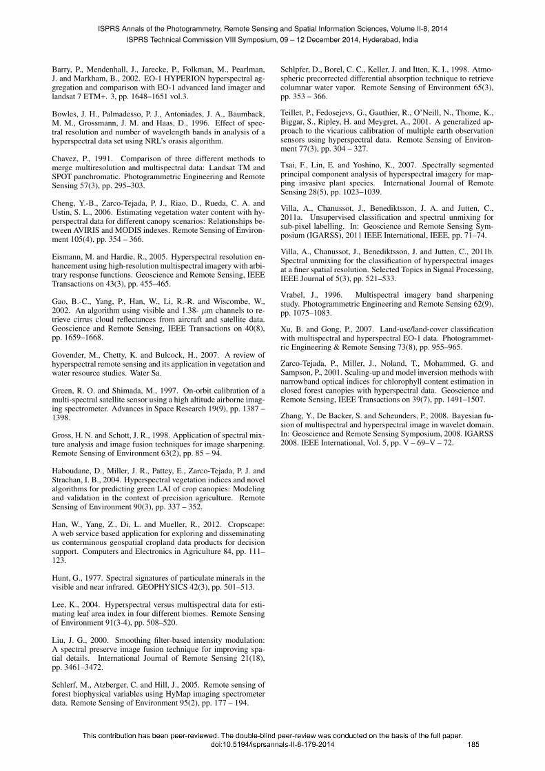
of a land cover class is essential. Hence, improvement in clas-sification should not be the only measure for evaluating spectralfidelity. Figure 7 shows the spectral signature of Wheat and Soy-abean. Vertical lines divides the signature into six sections, eachcorresponding to a multispectral band. As we can see from thefigure, both spectral signatures have subtle features(local mini-mas and maximas) that might be of interest in some applications.Hence, it is important to preserve these features in the fused prod-uct. Hence it is important that different algorithms maintain therelative ordering of values in spectral signatures and hence pre-serving these subtle features of the spectral signatures. Rankcorrelation measures the consistency between two given order-ings. In our case, we want to measure whether spectral signaturesfrom HySSVD are more consistent with true spectral signaturesor spectral signatures from PCA are more consistent. Here wehave used Kendall Tau rank correlation measure. Kendall Taucorrelation is defined as -

KT =

∑n−1

i=1

∑n

j=i+1sign((Bi −Bj)(Ii − Ij))∑n−1

i=1

∑n

j=i+11

(6)

where, B is the reference series of length n and I is the inputseries of length n. In words, KT measure the difference betweenthe number of concordant pairs and discordant pairs normalizedby total number of pairs. A pair of indices in the series are con-sidered concordant if both reference and input series increase ordecrease together from one index to other. Otherwise, the pair isconsidered discordant.

Table 4 shows class wise and overall rank correlation values onmixed pixels for different algorithms. From above table, we cansee that HySSVD has done a good job of preserving relative or-dering of values in the spectrum. For class Soyabean, HySSVDhas not shown any improvement but it has notably improved con-sistency for pixels of class Wheat. When compared with the base-line algorithm, PCA perform poorly than HySSVD. In order tounderstand these results in more detail, we plot the scatter plotof Kendall Tau value for different pairs of data images as shownin figure 8 and 9. In order to reduce number of plots, we havecompared HySSVD with only PCA.

Figure 9(a) compares HySSVD and PCA. As we can that the dis-tribution is mostly around the red line. This shows that both algo-rithm are performing similarly. But it is also important to see howmuch improvement has been made over the original hyperspectraldata (LR). Both algorithms have comparable performance withLR and hence there is not much gain for this class. Also, note thateven tough overall the points are distributed around the line but


0 0.2 0.4 0.6 0.8 10

0.2

0.4

0.6

0.8

1

HySSVD

PC

A

(a)

0 0.2 0.4 0.6 0.8 10

0.2

0.4

0.6

0.8

1

LR

HyS

SV

D

(b)

0 0.2 0.4 0.6 0.8 10

0.2

0.4

0.6

0.8

1

LR

PC

A

(c)

Figure 8: Scatter plot of Kendall Tau values for class Soyabean

Method Soyabean Wheat OverallFHS-PCA 0.93 0.85 0.91

FHS-HySSVD 0.94 0.89 0.92FHS-WAV 0.93 0.81 0.90

OHS 0.94 0.90 0.93

Table 5: Class wise Rank Correlation values for different meth-ods on pure pixels

PCA has more variance than HySSVD. This shows that PCA de-viates more from the original signature and has more propensityfor spectral distortion than HySSVD. For class wheat as shownin figure 9, HySSVD is performing better than PCA. At the sametime, HySSVD also shows slight improvement over LR. On theother hand, PCA is worse than the original data itself. This tellsus that PCA is more aggressive while doing enhancement anddeteriorates the relative spectral properties. For HySSVD we cansee that it performs very similar to LR which means that it is moreconservative and does not alter the LR spectrum very drasticallyand hence tends to avoid spectral distortion.

A similar analysis is required on pure pixels to ensure that thealgorithms are not introducing unwanted characteristics into thesignatures that do not need enhancement. Table 5 shows the per-formance on pure pixels.

Again, we can see that HySSVD has maintained the spectral char-acteristics of pure pixels more effectively than PCA. Figure 10shows anecdotal example of spectral distortion in pure and mixedpixels. Figure 10(a) shows spectral signature of the first 25 bandsof a pure pixel. We can see that the amount of distortion byHySSVD is minimal whereas PCA has introduced slight distor-tion in signature. Figure 10(b) shows spectral signature of the first25 bands of a mixed pixel. We can see that relatively large distor-tion of signature has happened in PCA based image. Even toughsignature from HySSVD is also different from required THS sig-nature but it has less distortion.

5. CONCLUSION

The paper presents a novel way of fusing hyperspectral data andmultispectral data to obtain an image with good characteristics

0 0.2 0.4 0.6 0.8 10

0.2

0.4

0.6

0.8

1

HySSVD

PC

A

(a)

0 0.2 0.4 0.6 0.8 10

0.2

0.4

0.6

0.8

1

LR

HyS

SV

D

(b)

0 0.2 0.4 0.6 0.8 10

0.2

0.4

0.6

0.8

1

LR

PC

A

(c)

Figure 9: Scatter plot of Kendall Tau values for class Wheat

5 10 15 20 251500

2000

2500

3000

Band Number

Pix

el V

alu

e

HySSVD

THS

PCA

OHS

(a) A Pure Pixel

5 10 15 20 25

500

1000

1500

2000

2500

3000

Band Number

Pix

el V

alu

e

HySSVD

THS

PCA

OHS

(b) A Mixed Pixel

Figure 10: Example Spectral signatures showing spectral distor-tion

of both. Each stage of the algorithm has many choices of subtechniques. For each stage a very fundamental technique hasbeen chosen as a proof of concept, in order to make the idea lesscomplex and easy to understand. Like most other algorithms, theperformance of the algorithm might decrease at larger resolutiondifferences due to upscaling of the data in the initial stage. Sincethe algorithm enhances only those hyperspectral bands which liein wide-band SRF ranges of the multispectral bands, this leavessome of the bands unsharpened. This is the tradeoff that has beenmade to maintain spectral integrity of the fused output. At theapplication level, this drawback will not be consequential as thealgorithm will give subsets of enhanced data in each region ofthe electromagnetic spectrum according to the SRFs of the mul-tispectral bands. This will allow correct classification and mate-rial identification capabilities. Comparison with a baseline algo-rithm shows that HySSVD has some potential of improving spa-tial quality while preserving spectral properties. Through exper-iments we showed that HySSVD has capability to improve per-formance in classification task. By careful analysis of the char-acteristics of the spectral signatures we demonstrated that base-line algorithm does distort spectral properties. The performanceof HySSVD is limited due to very conservative choice of vectordecomposition which does not alter original low resolution sig-nal drastically but this also prevents HySSVD from introducingspectral distortion.

ACKNOWLEDGEMENTS

We would like to thank NASA for the collection and free distri-bution of data from HYPERION and ALI sensor onboard EO-1satellite. We also thank NASA Agricultural Statistics Servicesfor providing high quality information land cover information ondifferent crops in USA.

REFERENCES

Slawomir Blonksi, Gerald Blonksi, Jeffrey Blonksi, Robert Ryan,Greg Terrie, Vicki Zanoni, 2001. Synthesis of multispectral bandsfrom hyperspectral data: Validation based on images acquired byaviris, hyperion, ali, and etm+. Technical Report SE-2001-11-00065-SSC, NASA Stennis Space Center.

Adam, E., Mutanga, O. and Rugege, D., 2010. Multispectral andhyperspectral remote sensing for identification and mapping ofwetland vegetation: a review. Wetlands Ecology and Manage-ment 18(3), pp. 281–296.

Amolins, K., Zhang, Y. and Dare, P., 2007. Wavelet based im-age fusion techniques an introduction, review and comparison.{ISPRS} Journal of Photogrammetry and Remote Sensing 62(4),pp. 249 – 263.


Barry, P., Mendenhall, J., Jarecke, P., Folkman, M., Pearlman,J. and Markham, B., 2002. EO-1 HYPERION hyperspectral ag-gregation and comparison with EO-1 advanced land imager andlandsat 7 ETM+. 3, pp. 1648–1651 vol.3.

Bowles, J. H., Palmadesso, P. J., Antoniades, J. A., Baumback,M. M., Grossmann, J. M. and Haas, D., 1996. Effect of spec-tral resolution and number of wavelength bands in analysis of ahyperspectral data set using NRL’s orasis algorithm.

Chavez, P., 1991. Comparison of three different methods tomerge multiresolution and multispectral data: Landsat TM andSPOT panchromatic. Photogrammetric Engineering and RemoteSensing 57(3), pp. 295–303.

Cheng, Y.-B., Zarco-Tejada, P. J., Riao, D., Rueda, C. A. andUstin, S. L., 2006. Estimating vegetation water content with hy-perspectral data for different canopy scenarios: Relationships be-tween AVIRIS and MODIS indexes. Remote Sensing of Environ-ment 105(4), pp. 354 – 366.

Eismann, M. and Hardie, R., 2005. Hyperspectral resolution en-hancement using high-resolution multispectral imagery with arbi-trary response functions. Geoscience and Remote Sensing, IEEETransactions on 43(3), pp. 455–465.

Gao, B.-C., Yang, P., Han, W., Li, R.-R. and Wiscombe, W.,2002. An algorithm using visible and 1.38- µm channels to re-trieve cirrus cloud reflectances from aircraft and satellite data.Geoscience and Remote Sensing, IEEE Transactions on 40(8),pp. 1659–1668.

Govender, M., Chetty, K. and Bulcock, H., 2007. A review ofhyperspectral remote sensing and its application in vegetation andwater resource studies. Water Sa.

Green, R. O. and Shimada, M., 1997. On-orbit calibration of amulti-spectral satellite sensor using a high altitude airborne imag-ing spectrometer. Advances in Space Research 19(9), pp. 1387 –1398.

Gross, H. N. and Schott, J. R., 1998. Application of spectral mix-ture analysis and image fusion techniques for image sharpening.Remote Sensing of Environment 63(2), pp. 85 – 94.

Haboudane, D., Miller, J. R., Pattey, E., Zarco-Tejada, P. J. andStrachan, I. B., 2004. Hyperspectral vegetation indices and novelalgorithms for predicting green LAI of crop canopies: Modelingand validation in the context of precision agriculture. RemoteSensing of Environment 90(3), pp. 337 – 352.

Han, W., Yang, Z., Di, L. and Mueller, R., 2012. Cropscape:A web service based application for exploring and disseminatingus conterminous geospatial cropland data products for decisionsupport. Computers and Electronics in Agriculture 84, pp. 111–123.

Hunt, G., 1977. Spectral signatures of particulate minerals in thevisible and near infrared. GEOPHYSICS 42(3), pp. 501–513.

Lee, K., 2004. Hyperspectral versus multispectral data for esti-mating leaf area index in four different biomes. Remote Sensingof Environment 91(3-4), pp. 508–520.

Liu, J. G., 2000. Smoothing filter-based intensity modulation:A spectral preserve image fusion technique for improving spa-tial details. International Journal of Remote Sensing 21(18),pp. 3461–3472.

Schlerf, M., Atzberger, C. and Hill, J., 2005. Remote sensing offorest biophysical variables using HyMap imaging spectrometerdata. Remote Sensing of Environment 95(2), pp. 177 – 194.

Schlpfer, D., Borel, C. C., Keller, J. and Itten, K. I., 1998. Atmo-spheric precorrected differential absorption technique to retrievecolumnar water vapor. Remote Sensing of Environment 65(3),pp. 353 – 366.

Teillet, P., Fedosejevs, G., Gauthier, R., O’Neill, N., Thome, K.,Biggar, S., Ripley, H. and Meygret, A., 2001. A generalized ap-proach to the vicarious calibration of multiple earth observationsensors using hyperspectral data. Remote Sensing of Environ-ment 77(3), pp. 304 – 327.

Tsai, F., Lin, E. and Yoshino, K., 2007. Spectrally segmentedprincipal component analysis of hyperspectral imagery for map-ping invasive plant species. International Journal of RemoteSensing 28(5), pp. 1023–1039.

Villa, A., Chanussot, J., Benediktsson, J. A. and Jutten, C.,2011a. Unsupervised classification and spectral unmixing forsub-pixel labelling. In: Geoscience and Remote Sensing Sym-posium (IGARSS), 2011 IEEE International, IEEE, pp. 71–74.

Villa, A., Chanussot, J., Benediktsson, J. and Jutten, C., 2011b.Spectral unmixing for the classification of hyperspectral imagesat a finer spatial resolution. Selected Topics in Signal Processing,IEEE Journal of 5(3), pp. 521–533.

Vrabel, J., 1996. Multispectral imagery band sharpeningstudy. Photogrammetric Engineering and Remote Sensing 62(9),pp. 1075–1083.

Xu, B. and Gong, P., 2007. Land-use/land-cover classificationwith multispectral and hyperspectral EO-1 data. Photogrammet-ric Engineering & Remote Sensing 73(8), pp. 955–965.

Zarco-Tejada, P., Miller, J., Noland, T., Mohammed, G. andSampson, P., 2001. Scaling-up and model inversion methods withnarrowband optical indices for chlorophyll content estimation inclosed forest canopies with hyperspectral data. Geoscience andRemote Sensing, IEEE Transactions on 39(7), pp. 1491–1507.

Zhang, Y., De Backer, S. and Scheunders, P., 2008. Bayesian fu-sion of multispectral and hyperspectral image in wavelet domain.In: Geoscience and Remote Sensing Symposium, 2008. IGARSS2008. IEEE International, Vol. 5, pp. V – 69–V – 72.


sensor simulation based hyperspectral image …

Documents