Joona Koskiahde

Decentralized Detection in RealisticSensor Networks

School of Electrical Engineering

Thesis submitted for examination for the degree of Master ofScience in Technology.

Espoo 26.12.2011

Thesis supervisor:

Prof. Andreas Richter

Thesis instructor:

D.Sc. (Tech.) Jan Eriksson

A! Aalto UniversitySchool of ElectricalEngineering

aalto-yliopistosahkotekniikan korkeakoulu

diplomityontiivistelma

Tekija: Joona Koskiahde

Tyon nimi: Hajautettu ilmaisu toteutettavissa langattomissa sensoriverkoissa

Paivamaara: 26.12.2011 Kieli: Englanti Sivumaara:8+54

Signaalinkasittelyn ja akustikan laitos

Professuuri: Signaalinkasittely Koodi: S-88

Valvoja: Prof. Andreas Richter

Ohjaaja: TkT Jan Eriksson

Tama tyo kasittelee kohteen ilmaisua sensoriverkolla, joka koostuu aanisensoreista.Tyon paapaino on epaideaalisen tilanteen kasittelylla, jossa monet hajautettuailmaisua kasittelevat oletukset, joita alan kirjallisuudessa tehdaan, eivat enaapade. Sensoriverkko koostuu mielivaltaiseen verkkotopologiaan asetetuistasensoreista ja fuusiokeskuksesta, ja tavoite on ilmaista verkkoa lahestyva kohde,joka tuottaa aanisignaalia. Tiedon kasittelyyn sensoreilla ja fuusiokeskuksellaesitetaan kaksi erilaista algoritmia. Toinen algoritmeista perustuu suurimmanuskottavuuden menetelmaan ja toinen on heuristinen, klassiseen ilmaisuteoriaanperustuva, lahestymistapa ongelmaan.

Algoritmien suorituskykya tutkitaan simulaatioiden avulla. Heuristisen algoritminsuorituskyky on huomattavasti parempi kaikissa simuloiduissa tilanteissa. Algo-ritmien johdossa taustakohina oletettiin normaalijakautuneeksi, mutta simulaa-tioiden perusteella algoritmit toimivat kohtuullisen hyvin myos pidempihantaisentaustakohinajakauman tapauksessa. Heuristinen algoritmi tarjoaa paremmansuorituskyvyn lisaksi myos helpomman tavan asettaa kynnysarvoparametrit niin,etta sensoreilla ja fuusiokeskuksella on haluttu vaaran halytyksen todennakoisyys.

Avainsanat: Hajautettu ilmaisu, Ilmaisuteoria, Sensoriverkot, Akustiset sen-sorit, Suurimman uskottavuuden menetelma

aalto universityschool of electrical engineering

abstract of themaster’s thesis

Author: Joona Koskiahde

Title: Decentralized Detection in Realistic Sensor Networks

Date: 26.12.2011 Language: English Number of pages:8+54

Department of Signal Processing and Acoustics

Professorship: Signal Processing Code: S-88

Supervisor: Prof. Andreas Richter

Instructor: D.Sc. (Tech.) Jan Eriksson

This thesis discusses the detection of a target using a network of acoustic sensors.The focus of the work is on considering what to do in a non-ideal situation,where many of the assumptions often made in decentralized detection literatureare no longer valid. The sensors and a fusion center are grouped in an arbitraryformation, and the object is to detect an approaching target which emits a soundsignal. Two different schemes are considered for processing the data at sensorsand the fusion center. One of the schemes is based on maximum likelihoodestimation and the other one is a heuristic approach based on classical detectiontheory.

The performances of the two schemes are studied in simulations. The heuristicscheme has a better detection performance for a given false alarm rate with alldifferent sets of settings for the simulation. In derivation of the schemes, the back-ground acoustic noise is assumed to be normal distributed, but, according to thesimulations, the schemes still work relatively well under a long tailed noise distri-bution. In addition to better performance, the heuristic scheme offers easier setupof threshold values and approximation of false alarm rates for given thresholdsusing simple equations.

Keywords: Decentralized detection, Distributed detection, Detection Theory,Sensor networks, Acoustic Sensors, Maximum likelihood

iv

Preface

I would like to thank my instructor D.Sc. (Tech.) Jan Eriksson and supervisor Prof.Andreas Richter for help with the subject matter and general tips for writing ascientific text. Also, special thanks go to Mr. Jari Nieminen for help with modelingwireless communications in simulations and my brother, Mr. Timo Koskiahde, forproofreading and comments on readability.

Otaniemi, 26.12.2011

Joona Koskiahde

v

Contents

Abstract (in Finnish) ii

Abstract iii

Preface iv

Contents v

List of symbols vii

1 Introduction 11.1 Sensor networks . . . . . . . . . . . . . . . . . . . . . . . . . . . . . . 11.2 Main scenario . . . . . . . . . . . . . . . . . . . . . . . . . . . . . . . 11.3 Objectives of the thesis . . . . . . . . . . . . . . . . . . . . . . . . . . 21.4 Organization of the thesis . . . . . . . . . . . . . . . . . . . . . . . . 2

2 Classical detection 32.1 Introduction . . . . . . . . . . . . . . . . . . . . . . . . . . . . . . . . 32.2 Neyman–Pearson theorem . . . . . . . . . . . . . . . . . . . . . . . . 42.3 Composite hypothesis testing . . . . . . . . . . . . . . . . . . . . . . 5

3 Decentralized detection 63.1 Introduction . . . . . . . . . . . . . . . . . . . . . . . . . . . . . . . . 63.2 Censoring . . . . . . . . . . . . . . . . . . . . . . . . . . . . . . . . . 73.3 Maximum likelihood detection . . . . . . . . . . . . . . . . . . . . . . 9

4 Decentralized detection of vehicle noise in a forest 114.1 Introduction . . . . . . . . . . . . . . . . . . . . . . . . . . . . . . . . 114.2 Practical considerations . . . . . . . . . . . . . . . . . . . . . . . . . 114.3 Sensors’ decision rules . . . . . . . . . . . . . . . . . . . . . . . . . . 13

4.3.1 Maximum likelihood scheme . . . . . . . . . . . . . . . . . . . 134.3.2 Classical composite hypothesis testing approach . . . . . . . . 14

4.4 Fusion center decision rule . . . . . . . . . . . . . . . . . . . . . . . . 174.4.1 Maximum likelihood scheme . . . . . . . . . . . . . . . . . . . 174.4.2 Combining standard deviations . . . . . . . . . . . . . . . . . 18

4.5 Further considerations . . . . . . . . . . . . . . . . . . . . . . . . . . 22

5 Special characteristics of other scenarios 245.1 Detecting impulses . . . . . . . . . . . . . . . . . . . . . . . . . . . . 245.2 Scenarios without a fusion center . . . . . . . . . . . . . . . . . . . . 245.3 Direct communication with the fusion center . . . . . . . . . . . . . . 245.4 Different types of sensors . . . . . . . . . . . . . . . . . . . . . . . . . 255.5 Target localization and tracking . . . . . . . . . . . . . . . . . . . . . 25

vi

6 Simulations 276.1 Simulation scenario . . . . . . . . . . . . . . . . . . . . . . . . . . . . 276.2 Modeling sound propagation in a forest . . . . . . . . . . . . . . . . . 286.3 Wireless communication model . . . . . . . . . . . . . . . . . . . . . 306.4 Default settings for the simulation . . . . . . . . . . . . . . . . . . . . 316.5 Simulation 1 — Performance at different rates of PFA . . . . . . . . . 336.6 Simulation 2 — Different noise distribution . . . . . . . . . . . . . . . 346.7 Simulation 3 — Binary sensors . . . . . . . . . . . . . . . . . . . . . 38

6.7.1 Introduction . . . . . . . . . . . . . . . . . . . . . . . . . . . . 386.7.2 Main scenario . . . . . . . . . . . . . . . . . . . . . . . . . . . 396.7.3 Linear array . . . . . . . . . . . . . . . . . . . . . . . . . . . . 39

6.8 Simulation 4 — Effect of β . . . . . . . . . . . . . . . . . . . . . . . . 406.8.1 Introduction . . . . . . . . . . . . . . . . . . . . . . . . . . . . 406.8.2 Main scenario . . . . . . . . . . . . . . . . . . . . . . . . . . . 406.8.3 Linear array . . . . . . . . . . . . . . . . . . . . . . . . . . . . 41

6.9 Discussion of simulation results . . . . . . . . . . . . . . . . . . . . . 42

7 Conclusions and future work 447.1 Conclusions . . . . . . . . . . . . . . . . . . . . . . . . . . . . . . . . 447.2 Directions of future work . . . . . . . . . . . . . . . . . . . . . . . . . 44

References 46

Appendix A — Matlab simulation script 50

vii

List of symbols

A attenuation of a sound signal in decibelsAatm attenuation of a sound signal due to atmospheric absorptionAbar attenuation of a sound signal due to a barrierAgr attenuation of a sound signal due to the ground effectAdiv attenuation of a sound signal due to geometrical divergenceAmisc attenuation of a sound signal due to miscellaneous effectsAi signal of the target at sensor iα a multiplier in the decision rule of the fusion center in the max-

imum likelihood schemeαs attenuation parameter of the atmospheric absroptionB number of sensors that have something to send at a given timeβ multiplier for the decision rule of the fusion center in the com-

bining standard deviations schemed distance a sound propagates in the aird0 reference distance of 1 mDc directivity correction in decibelsf(xi) a function of the measurements of sensor iγ threshold of a likelihood ratio testγ0 threshold of the decision rule of the fusion centerγi threshold of a likelihood ratio test of sensor iγ′i threshold to which test statistic T (xi) is comparedΓ(x) gamma functionH0 null hypothesis, target absent hypothesisH1 alternative hypothesis, target present hypothesisi sensor indexk sensor measurement indexkG shape parameter of a gamma distributionK number of measurements the sensors take into account in their

decision rulel(x;H0) likelihood function of the measurements under H0

l(x;H1) likelihood function of the measurements under H1

LfT (DW ) continuous downwind octave-band sound pressure levelLP sound pressure level at a sensor due to the targetLP1m sound pressure level at 1 m from the sourceLW sound power level of the sourceΛ(x) likelihood ratioΛi(xi) likelihood ratio at sensor i

Λi(xi) likelihood ratio at sensor i with estimated likelihoodsM binomially distributed random variableµ expected value of a random variableµi expected value of the measurements of sensor iµ0,i expected value of the measurements of sensor i under H0

viii

µ1,i expected value of the measurements of sensor i under H1

µ0,i estimate of µ0,i

N number of sensors in the networkN (µ, σ2) normal distribution with parameters µ and σ2

p probability with which each of the B sensors transmit in a timeslot

popt approximately optimal value for pp(x) probability density functionp(x;H0) probability density function of measurements under H0

p(x;H1) probability density function of measurements under H1

φ0(φ1, . . . , φN) decision rule of the fusion center

φ0(φ1, . . . , φN) decision rule of the fusion center in the maximum likelihoodscheme

φi(xi) local decision rule of sensor i

φi(xi) local decision rule of sensor i in the maximum likelihood schemePD probability of detectionPFA probability of false alarmPM probability of missPSNR probability that a packet sent from a sensor is lost due to a low

signal-to-noise ratioΦ(x) cumulative distribution function of the standard normal distri-

butionQ(x) Q-function, complementary cumulative distribution function of

the standard normal distributionQ−1(x) inverse Q-functionρ value associated with the censoring region of the sensorsρi value associated with the censoring region of sensor iS number of time slots in an active periodσ2i variance of the background noise distribution at sensor iσ2i estimate of σ2

i

θG scale parameter of a gamma distributionT (xi) test statistic of the combining standard deviations schemex a single measurementxi[k] a single measurement of sensor ix vector of measurementsxi vector of measurements of sensor iyi(xi) normalized measurements of sensor i

1 Introduction

This thesis focuses on detecting a target with a network of sensors. The generalintroductions to sensor networks and the situation under consideration are given inthis chapter. Additionally, organization of topics and objectives of the thesis arediscussed.

1.1 Sensor networks

Sensor networks consist of sensors which measure some physical properties of theenvironment and are able to communicate with each other. The sensors are usuallybattery-powered and equipped with low-power computing hardware, and a radiotransceiver [1]. Typically, there is also a node with heavier computing capabilitiesin the network called a fusion center, which is used to combine information from thesensors [2].

Energy consumption is an important aspect in the design of sensor networkssince the sensors usually operate on battery-power. Therefore, smaller energy con-sumption results in longer lifetime of the network. This should be taken into accountin all levels of design. Applications should generate little traffic into the network,network layer packets should have minimum overhead, and radios should transmitat moderate power levels.

There are numerous military and civil scenarios where sensor networks may beutilized. Deployed on the battlefield, a sensor network can detect, classify, and trackenemy movements. In environmental studies, a sensor network can be used for, e.g.,habitat monitoring or measuring temperature, wind speed, and humidity. [3]

1.2 Main scenario

In surveillance applications, the first and often the most critical step is detection ofan intruder or a target. Naturally, if a target is to be classified, localized, or tracked,it must be detected first. In this thesis, the focus is on detecting a target using asensor network. The main scenario considered is detection of a vehicle in a forestusing acoustic sensors. This scenario could arise, e.g., in a military setting where asensor network is deployed along a forest road to give an alarm if unknown vehiclesmove on the road.

In designing a good way to process the measurements from the sensors to detectthe target, attention is turned to detection theory. Some basic principles and defi-nitions are described from classical detection theory. Fundamentals of decentralizeddetection are also presented, where part of the decision making process is distributedto the sensors.

Although the vehicle could be detected with, e.g., seismic sensors [4], acousticsensors are discussed here since the propagation of sound and hearing the targetare relatively easy to understand intuitively. It should be clear that basic conceptsof decision theory apply just as well to seismic and other types of measurementssimilarly to acoustic measurements.

2

1.3 Objectives of the thesis

The purpose of this thesis is to devise a suitable detection scheme for the main sce-nario described above. The reasons why many of the schemes presented in detectionliterature are not suitable for this scenario are discussed. Two different approachesto the problem of the main scenario are considered, and their performances arecompared in simulations. Both approaches have parameters which need to be set.Methods to find practical values for these parameters are discussed, as well.

1.4 Organization of the thesis

Classical centralized detection is described in Chapter 2. In Chapter 3, decentralizeddetection with a sensor network is discussed. How to apply the theory of classical anddecentralized detection to practical scenarios, especially the main scenario describedin Chapter 1.2, is considered in Chapter 4. Chapter 5 highlights some characteristicsof other scenarios that are related to the main scenario. To find out the performanceof the proposed detection algorithms, a number of simulations were run. Thesesimulations and their results are described in Chapter 6. Chapter 7 concludes thethesis and proposes directions for future research.

3

2 Classical detection

This chapter is an introduction to classical detection theory. In classical detectiontheory, only a single sensor and its measurements are considered. Some basic con-cepts and terminology are discussed here. These are needed later when the problemof the main scenario is discussed in detail.

2.1 Introduction

In the main scenario (Chapter 1.2) the objective is to infer if a target is absentor present in the network. The target emits a sound signal, and based on soundmeasurements a decision has to be made on absence or presence of the target. Mea-surements are perturbed by random background noise which makes the detectionof the target signal nontrivial. Detecting a signal in noise is essentially a statisticalhypothesis testing problem [5]. Absence or presence of the target correspond tonull hypothesis (H0) and alternative hypothesis (H1), respectively. This is a binaryhypothesis testing problem since there are only two different hypotheses.

Since measurements are disturbed by random background noise, the measure-ments are modeled as random variables. Under each hypothesis, H0 and H1, themeasurements have a different distribution, e.g., the target signal may increase themean of the distribution of background noise. In detection, the objective is to inferfrom which distribution the measurements are drawn. Since the background noise isusually modeled as a continuous distribution, a fixed set of measurements may havebeen generated by both distributions. Therefore, there is a possibility of making anerror in the inference. A decision can be made that the target is present, althoughit is not, or, on the other hand, a decision can be made that there is no target,although there is one. The probability of deciding the target is present, even thoughit is not, is called the probability of false alarm (PFA). The probability of decidingthe target is absent, even though there is one, is called the probability of miss (PM).The probability of making a correct decision when the target is present is called theprobability of detection (PD). Notice that PD = 1− PM .

Figure 1 illustrates a case where there is only one measurement. Probabilitydensity functions of the measurements under H0 and H1 are denoted by p(x;H0)and p(x;H1), respectively. The figure illustrates a decision rule which decides infavor of H1 when x > 2. The probability of detection equals the green area, andthe probability of false alarm equals the red area. It should be obvious from thefigure that PFA can decreased by moving the threshold right, but at the same timePD decreases. Conversely, both PD and PFA can be increased at the same timeby moving the threshold left. This is due to the fact that PFA and PD cannot beadjusted to opposing directions at the same time by adjusting the threshold [5].

Naturally, a good detector has a high PD and a low PFA. A detector thatmaximizes PD for a given PFA, assuming the distributions under both hypothesesare completely known, is described next.

4

−4 −2 0 2 4 60

0.1

0.2

0.3

0.4

x

Values

ofthePDFs

p(x;H0)p(x;H1)PDPFA

Figure 1: Probabilities of detection and false alarm for two example distributionsusing only one measurement x.

2.2 Neyman–Pearson theorem

The Neyman–Pearson (NP) theorem [6] states that to maximize the probability ofdetection (PD) for a given probability of false alarm (PFA), decide H1 if

Λ(x) =l(x;H1)

l(x;H0)> γ, (1)

where x is the vector of measurements, l(x;H0) and l(x;H1) are the likelihoodfunctions of the measurements under H0 and H1, respectively, and γ is the thresholdwhich satisfies the given PFA. The likelihood function is effectively the same asthe probability density function of the measurements, i.e., l(x) = p(x), only theinterpretation is different. In the probability density function, the variable is x, andthe parameters of the distribution are fixed. In the likelihood function, the variablesare the parameters of the distribution, and x is fixed. Since Λ(x) is the ratio ofthe likelihoods of H1 and H0, it is called the likelihood ratio. The whole test (1),including both the likelihood ratio and the threshold, is termed the likelihood ratiotest (LRT).

The value of the threshold γ can be obtained from the following relations between

5

γ and PFA

PFA = Pr {Λ(x) > γ;H0} =

∫

{x:Λ(x)>γ}l(x;H0) dx, (2)

where the notation x : Λ(x) > γ indicates the region of x where Λ(x) > γ [5].

2.3 Composite hypothesis testing

In the discussion above, it was assumed that the distributions of the measurementsunder both hypotheses are completely known. The scenario is termed simple hy-pothesis testing. If the distributions contain unknown parameters, the problem iscalled composite hypothesis testing. This is more akin to the main scenario (Chapter1.2) where the objective is to detect a sound signal of unknown amplitude in noise.The first approach to designing a test for distributions containing unknown param-eters is to design an NP test (1) assuming the unknown parameters are known. Thetest should be then modified so that it does not depend on the unknown parametersanymore, if possible. The resulting test is optimal in the Neyman-Pearson sensesince it is an NP test. Another approach is to build the so-called generalized like-lihood ratio test. In the generalized likelihood ratio test, the unknown parametersin the distributions are first estimated, and then the distributions are used in thelikelihood ratio test with the estimated parameters. [5]

6

3 Decentralized detection

Instead of the situation of a single sensor of the previous chapter, detection withseveral sensors is considered in this chapter. This gives rise to a new problem offusing the information from the sensors. Also, a method to save significant amountsof energy in this type of situation is discussed.

3.1 Introduction

In classical detection of Chapter 2, only one sensor, which makes a decision based onits own measurements, is considered. By contrast, in centralized and decentralizeddetection, a network of sensors is considered [7]. In centralized detection, the sensorssimply send all their raw data to the fusion center for decision making. This maybe unnecessary at times and requires constant communication between the sensorsand the fusion center. Thus, in decentralized detection, the sensors have their ownlocal decision rules that define what and when to send to the fusion center [8],which combines the information it receives from the sensors. The sensors mightnot always send something, and when they send, they do not necessarily send theirmeasurements as such but some function of the measurements.

In the rest of this thesis, decentralized detection is disscussed instead of central-ized detection, since a centralized setting can be thought of as a special case of adecentralized setting. The fusion center has its own decision rule which determineshow to make a decision about the absence or presence of the target based on theinformation received from the sensors. This is illustrated in Figure 2. Signal fromthe target at sensor i is denoted by Ai, xi are the measurements of sensor i, andf(xi) is its function of the measurements that is sent to the fusion center if thesensor decides the target is present. In this representation, the left switch is closedwhen the target is present in the network, and the right switch is closed when thecorresponding sensor decides the target is present. Thus, a sensor’s objective is toclose the right switch when the left switch is closed, and vice versa. A sensor makesthis decision based on its noise-corrupted measurements.

Classical detection could, in principle, be employed in a network of sensors.Then, there would be no fusion center, and any single sensor could set off the alarm.The performance of the system would be worse than in a decentralized system sinceall information would not be used in the decision making. This can be intuitivelyunderstood if sensors are thought to gather evidence of the target. If one sensor hasconclusive evidence of the target or several sensors have a weak piece of evidence ina decentralized setting, the fusion center sets off the alarm. In a classical type ofsystem the situation where several sensors have weak, but not conclusive, evidencewould not set off the alarm. One might want to compensate for this by setting thesensors to give an alarm already if it has some weak evidence, but this would alsoincrease the rate of false alarms.

In early papers that discussed decentralized detection, mainly quantization ofmeasurements or likelihood ratios was considered, and sensors sent some informa-tion to the fusion center all the time [2, 9]. From the viewpoint of total energy

7

Figure 2: Setup of a decentralized detection scenario.

consumption of the sensors, quantization of measurements which are transmittedat a low data rate is not significant. Packet lengths used by the sensors’ radiosare typically longer than the amount of bits required to accurately represent thefunction of measurements in question, and communication protocols often requiretransmission of side information [10, 11]. Additionally, starting a transmission withradio hardware may consume significant amounts of energy [12]. Thus, in this the-sis, energy efficiency is considered by reducing the number of transmissions, not thesize of transmissions. The loss in performance due to quantization also becomes in-significant quickly as the number of quantization levels increases from the minimumof two [7].

3.2 Censoring

Saving the limited battery power of the sensors is important, since energy consump-tion is related to the lifetime of the network. If the null hypothesis is significantlymore likely, as in the main scenario (Chapter 1.2), sending messages saying the tar-get is absent all the time is not informative. Large amounts of energy can be savedby not sending anything from the sensors to the fusion center when the target is notobserved. This is called censoring.

In considering what the sensors should send to the fusion center, when theysend, an assumption is made. Measurements are assumed to be conditionally in-dependent from all other sensors’ measurements, conditioned on both hypotheses.This assumption is satisfied under the null hypothesis for local noise [13], especiallyif the sensors are not too close to each other. This assumption might not hold verywell when the target is present in some cases [14]. However, this assumption is madeto keep the expressions tractable. The complexity of designing optimal detection

8

algorithms becomes an extensive problem without this assumption [15].Conditionally independent measurements lead to computing [16] and censoring

[17] likelihood ratio tests at the sensors. Each sensor should compute its locallikelihood ratio according to equation (1), i.e., assuming N sensors in the network,for each sensor i, i = 1 . . . N , the likelihood ratio is

Λi(xi) =l(xi;H1)

l(xi;H0), (3)

where xi are the conditionally independent and identically distributed measurementsof sensor i.

This likelihood ratio (3) should be sent to the fusion center only if it is largeenough. It is not obvious that censoring the likelihood ratio when it is smaller thansome threshold value is optimal. It is not even obvious that the optimal censoringregion should be a single interval. Fortunately, it has been shown that under somemild conditions, the optimal censoring interval is a single interval which has a lowerthreshold of zero [17]. Thus, for each sensor i, the local decision rule is

φi(xi) =

{Λi(xi), if Λi(xi) ≥ γi,ρi, if Λi(xi) < γi,

(4)

where γi is the threshold to which the likelihood ratio is compared, and ρi is thevalue associated with the censoring region. This value associated with the censoringregion, ρi, is needed later when a decision rule for the fusion center is designed.Notice that, according to the censoring principle, nothing is sent to the fusion centerif Λi(xi) < γi, although ρi is a value associated with this region of Λi(xi). Thethreshold, γi, can be used to adjust the sensitivity of the sensor i, determining howlarge the measurements must be before making a local decision of presence of thetarget and sending the likelihood ratio to the fusion center.

The fusion center has a decision rule which it uses to decide if the target ispresent or absent in the network. Given the local sensor decision rules (4), theoptimal decision rule for the fusion center is [17]

φ0(φ1, . . . , φN) =

{1, if

∏Ni=1 φi(xi) ≥ γ0,

0, otherwise,(5)

where 1 and 0 correspond to deciding the target is present or absent for the network,respectively, and γ0 is the decision threshold for the fusion center that can be usedto adjust the sensitivity of alarms. Factors of

∏Ni=1 φi(xi) which are not received

from sensors correspond to the censored likelihood ratios. As defined in equation(4), they correspond to ρi. They are evaluated at the fusion center as

ρi =Pr {Λi < γi;H1}Pr {Λi < γi;H0}

. (6)

However, there is a problem if this sceme is applied to the main scenario (Chapter1.2). Distribution of the measurements under the target hypothesis is unknown,

9

since the distance of the target from each sensor is unknown. I.e., l(xi;H1) is notcompletely known since it depends on the loudness of the target and the distanceof the target from sensor i. The form of l(xi;H1) is assumed to be known, but atleast one parameter is not known. Therefore, the likelihood ratios at the sensors,and the unreceived, censored likelihood ratios at the fusion center cannot be eval-uated. However, the distribution of background noise, p(xi;H0), is assumed to becompletely known. This means the estimates of mean (11) and variance (12) inChapter 4.2 are assumed to be so good that their errors can be ignored.

3.3 Maximum likelihood detection

To overcome the problem of not knowing p(xi;H1) completely, the unknown param-eter can be estimated using the maximum likelihood principle, and this estimatecan be used in the likelihood ratio (3). This approach to hypothesis testing is alsocalled the generalized likelihood ratio test [5]. In maximum likelihood detection, themaximum likelihood estimate of the unknown parameter in p(xi;H1) is computedat each sensor [13].

Maximum likelihood estimation is widely used in practical estimation problems,since it is relatively simple and can often be found quite easily. In general, themaximum likelihood estimate of a parameter µ of a probability density functionp(x), where x are samples from the distribution depending on µ, is the value ofµ that maximizes p(x) for a fixed x. This can be understood intuitively as thevalue of µ that is most likely to have produced the observations x. However, for afinite number of observations, the maximum likelihood estimator has no optimalityproperties. [20]

Maximum likelihood estimation procedure can be applied here, since l(xi;H1)and l(xi;H0) are essentially probability density functions, as discussed in Chapter2.2. Assume that l(xi;H1) and l(xi;H0) differ only in one parameter, their expectedvalue, µi. Under H0, the parameter is assumed to be known, µi = µ0,i. This meansthe sensors are assumed to know the expected value of their measurements, whenthere is no target but only background noise. Notice that in reality µ0,i has to beestimated, too, with the estimator given in equation (11). This estimate is assumedto be obtained from such a large amount of data that the estimation error can beignored, and µ0,i is assumed to be known. Under H1, the parameter µi is unknown,but it is assumed to be larger than µ0,i. This is a natural assumption since theadditional signal from the target increases the expected value of the measurements.The maximum-likelihood estimate of l(xi;H1) can be found by maximizing l(xi;H1)over the parameter µi. Therefore, instead of using the classical likelihood ratio (3)at each sensor, each sensor computes

Λi(xi) =maxµi

l(xi;H1)

l(xi;H0), (7)

10

and uses Λi(xi) in the decision rule (4), yielding

φi(xi) =

{Λi(xi), if Λi(xi) ≥ γi,

ρi, if Λi(xi) < γi.(8)

The fusion center may use a decision rule similar to the one in equation (5) whichmultiplies the received and censored likelihood ratios together, i.e.,

φ0(φ1, . . . , φN) =

{1, if

∏Ni=1 φ(xi) ≥ γ0,

0, otherwise.(9)

However, there is still the same problem as in Chapter 3.2: the fusion center wouldneed ρi, corresponding to censored likelihood ratios, to evaluate the right side ofequation (9). The fusion center cannot evaluate it from equation (6) since it doesnot know the distribution under H1. Unlike the sensors, it cannot estimate theunknown parameter in the distribution under H1, since the fusion center does nothave the measurements of sensor i. It is proposed in [13] that the fusion centershould set ρi = γi to provide robustness to uncertainty in the unknown parameterof the distribution under H1. This requires that the fusion center knows γi so thesensors must inform the fusion center of the threshold they use in their decision rule(8).

11

4 Decentralized detection of vehicle noise in a for-

est

Whereas the two previous chapters dealt mainly with the theory of detection, thischapter focuses on applying the theory to the main scenario. This chapter considersin detail how the sensors and the fusion center should process their information.Two different approaches are proposed for both the sensors and the fusion center.

4.1 Introduction

From viewpoint of a single sensor, the problem of the main scenario (Chapter 1.2) isessentially a detection of an unknown but positive mean shift in noise. This is exactlythe composite hypothesis testing problem described in Chapter 2.3. Therefore, itwould make sense to treat the problem at the sensor as a composite hypothesistesting problem and to design some associated fusion rule for the fusion center. Asdiscussed in Chapter 3, according to the censoring paradigm, the sensors considerwhether or not to send information to the fusion center. This can be interpreted asa local decision on the absence or presence of the target, but a single sensor decidingthe target is present does not start an alarm in the network. When a sensor decidesthe target is present, it sends some function of its measurements to the fusion center.The decision making of the sensors in the network is discussed in Chapter 4.3.

The fusion center needs some rule according to which it uses the received infor-mation to make the final decision on absence or presence of the target. The decisionrules for the fusion center that are optimal in some sense, some of which were dis-cussed in Chapter 3, often include an assumption that all sensors observe the samephenomena independently. In the main scenario, the sensors are spread across sucha wide area that this assumption is not valid when the target is present. If this weretaken into account, the tractability of the expressions for the decision rules mightbecome an issue. Regardless of that, some sort of decision rule for the fusion centerhas to be designed. Decision rules for the fusion center are discussed in Chapter 4.4.

4.2 Practical considerations

The acoustic sensors used are assumed to be simple omnidirectional microphoneswhich measure sound pressure. The measurements considered in this thesis aremeasurements of effective sound pressure. Effective sound pressure is the root meansquare over a set of instantaneous sound pressure measurements. This set of instan-taneous sound pressure measurements is assumed to be taken over a time period,which is short enough that the characteristics of the background noise and targetsignal stay approximately the same, but long enough that it encompasses severalwavelengths in the frequency range of interest. For example, this time period couldbe 200 ms.

The acoustic background noise, which affects the instantaneous sound pressuremeasurements, consists of sounds from a large number of sources such as rustlingof leaves in the surrounding trees. In other words, the background noise is a sum

12

of many sources of acoustic noise. The central limit theorem states that the sumof several independent random variables converges to a normal distribution as thenumber random variables in the sum grows to infinity [18]. The individual randomvariables in the sum need to have a finite expected value and a finite variance,but as long as these are finite, the distributions of the random variables can bearbitrary. Therefore, according to the central limit theorem, the background noiseof the instantaneous sound pressure measurements can be approximated by a normaldistribution.

As discussed above, the effective sound pressure measurements are root meansquares of sets of normal distributed random variables. Therefore, they are chidistributed. Again invoking the central limit theorem, if there are enough measure-ments in the set, the chi distribution can be approximated with a normal distribu-tion. In the design of the sensors’ decision rules, the acoustic background noise inthe forest is modeled by a normal distribution with mean µ0,i and variance σ2

i . I.e.,each effective sound pressure measurement, henceforth just measurement, in xi atsensor i, xi[k], k = 1 . . . K, is distributed as

xi[k] ∼{

N (µ0,i, σ2i ) under H0,

N (µ0,i + Ai, σ2i ) under H1,

(10)

where Ai is the unknown mean shift depending on the loudness of the target andits distance from sensor i. While the normality assumption might not hold in, e.g.,windy conditions, there is some justification for the assumption [19]. Furthermore,measurements xi[1] . . . xi[K] are assumed to be identically and independently dis-tributed for a fixed i, i.e., for each sensor individually. This means that, undereach hypothesis, each measurement in the set xi[1] . . . xi[K] at sensor i is drawnfrom the same normal distribution having the same µ0,i, σ

2i , and Ai. If the target

moves between the measurements, the target signal strength Ai changes and, strictlyspeaking, the assumption does not hold anymore. However, the K measurementsare assumed to be taken during such a short time interval that the change in Ai isnegligible.

Naturally, the sensors do not know µ0,i and σ2i , but each sensor can estimate

them by taking measurements when the network is initialized. If a sensor takes Kmeasurements x[k], k = 1 . . . K, it can estimate µ as

µ0,i =1

K

K∑

k=1

x[k] (11)

and σ2i as

σ2i =

1

K − 1

K∑

k=1

(x[k]− µ0,i)2. (12)

It can be shown that these estimators for the expected value and variance of anormal distribution are actually mimimum variance unbiased estimators for theseparameters [20]. This means they have the smallest variance among all unbiasedestimators of these parameters. Thus, the expected value of the squared error ofthese estimates is the smallest among all unbiased estimators of these parameters.

13

4.3 Sensors’ decision rules

Two different schemes for processing the measurements in sensors are presented inthis chapter. The first scheme is based on maximum likelihood estimation, and thesecond scheme is derived from classical detection theory.

4.3.1 Maximum likelihood scheme

If the maximum likelihood scheme of Chapter 3.3 is to be used in the detectionproblem, each sensor needs to compute the maximum likelihood estimate of theirlikelihood ratio (7). Since the measurements are assumed to be distributed accordingto equation (10), computing the estimated likelihood ratio (7) includes maximizing

l(xi;H1) =1

(2πσ2i )

K2

e− 1

2σ2i

∑Kk=1(xi[k]−µ1,i)2

(13)

with respect to µ1,i = µ0,i + Ai, i.e., the expected value of the measurements whenthe target is present. The sensors do not know µ1,i, but they compute the maximumlikelihood estimate of it, so that it can be used in computing the estimated likelihoodratio (7). This estimate is derived next. The general outline of the derivation follows[20, pp. 163–164].

Natural logarithm is a strictly increasing function, so the natural logarithm of afunction attains is maximum value at the same point where the original function at-tains its maximum value. Thus, instead of the likelihood funcion (13), its logarithmcan be maximized,

ln l(xi;H1) = ln

(1

(2πσ2i )

K2

e− 1

2σ2i

∑Kk=1(xi[k]−µ1,i)2

)(14)

= − ln(

(2πσ2i )

K2

)− 1

2σ2i

K∑

k=1

(xi[k]− µ1,i)2. (15)

The extrema of a function are found at the points where the derivative equals zeroor at the end points of domain of the function. Finding the maxima of ln l(xi;H1)with respect to µ1,i is considered next. The expected value of a normal distribution,µ1,i, can take any values in the range (−∞,∞). Clearly ln l(xi;H1) −→ −∞ asµ1,i −→ ∞ or µ1,i −→ −∞. The function to be maximized, ln l(xi;H1), is alogarithm of a probability density function, so ln l(xi;H1) ≥ 0. Thus, it has tohave at least one maximum inside the endpoint of its domain. The extrema insidethe domain are found in the points where the derivative equals zero. Taking thederivative with respect to µ1,i gives

∂ ln l(xi;H1)

∂µ1,i

=1

σ2i

K∑

k=1

(xi[k]− µ1,i) =1

σ2i

(K∑

k=1

xi[k]−Kµ1,i

). (16)

Setting this to zero, denoting the estimate of µ1,i as µ1,i, and solving for µ1,i yields

µ1,i =1

K

K∑

k=1

xi[k]. (17)

14

To make sure this is the maximum and not the minimum, the sign of the secondderivative is checked. Differentiating function (16) again with respect to µ1,i gives

∂2 ln l(xi;H1)

∂µ21,i

= −Kσ2i

. (18)

Since K and σ2i are positive, equation (18) is always negative. Thus, equation(17)

gives the maximum, and replacing µ1,i with its estimate (17) maximizes equation(13). In this scheme, if a sensor decides the target is present, it sends its estimatedlikelihood ratio (7) to the fusion center.

There is an important distinction between equations (11) and (17), althoughboth are sample averages. The estimate of the average level of acoustic backgroundnoise (11) is computed once when the network is initialized and no target is presentin the network. If necessary, it may be updated, for instance, if it begins to rain, thebackground noise level grows, but in any case its value changes rarely. On the otherhand, the estimate in equation (17) is computed in every time step as the sensormakes a decision on presence or absence of the target.

In addition of maximizing function (13), ρi and γi in function (8) have to be set.It is not simple to determine them so that they would yield a certain probability offalse alarm. In this thesis, a computer simulation is used to determine the parametersto yield a suitably low rate of false alarms. If ρi = γi is set, as suggested in Chapter3.3, and the same value of ρi is set to all sensors, then all sensors are set to the sameprobability of false alarm assuming the same background noise conditions. In thissituation, Matlab [21] script of Appendix A can be used to find a suitable value forthe parameter ρ.

4.3.2 Classical composite hypothesis testing approach

With the assumption of normal distributed background noise, the problem at eachsensor is essentially that of detecting an unknown but positive mean shift in Gaussiannoise. This is a special case of the classical composite hypotesis problem of Chapter2.3. As discussed in Chapter 2.3, first a Neyman–Pearson test (1), or NP test, isdesigned as if the value of the mean shift were known, and then the test is modifiedso that it does not depend on the value of the mean shift. Next, an NP test (1) isderived for this setting. The derivation follows the outline of the derivation in [5,pp. 191–194]. In this case, the NP test decides the target is present if

Λi(xi) =l(xi;H1)

l(xi;H0)=

1

(2πσ2i )K2e− 1

2σ2i

∑Kk=1(xi[k]−(µ0,i+Ai))

2

1

(2πσ2i )K2e− 1

2σ2i

∑Kk=1(xi[k]−µ0,i)2

> γi, (19)

since the joint probability density function of xi under each hypothesis is the productof the marginal probability density functions of the measurements xi[k]. To be exact,µ0,i should be replaced in the equation (19) with its estimate, µ0,i. However, thevalue of this estimate is assumed to be so close to the true value that its true valuecan be used in the equation.

15

Combining the exponentials and canceling out common terms yields

e− 1

2σ2i

(−2Ai∑Kk=1 xi[k]+K(A2

i+2µ0,iAi))> γi. (20)

Taking the natural logarithm of both sides gives

− 1

2σ2i

(− 2Ai

K∑

k=1

xi[k] +K(A2i + 2µ0,iAi)) > ln(γi). (21)

Rearranging the equation yields

Ai

K∑

k=1

xi[k] > σ2i ln(γi) +

K

2(A2

i + 2µ0,iAi). (22)

Since the target signal Ai is positive at each sensor, both sides can be divided byAi, and the inequality still holds, resulting in

K∑

k=1

xi[k] >σ2i

Ailn(γi) +

K

2(Ai + 2µ0,i). (23)

Scaling by 1/K yields to the test statistic

T (xi) =1

K

K∑

k=1

xi[k] >σ2i

KAiln(γi) +

1

2(Ai + 2µ0,i) = γ′i, (24)

where γ′i denotes the threshold to which the test statistic is compared.The test statistic does not depend on Ai, but the threshold appears to depend

on it. If that would really be the case, the test could not be implemented, sinceAi would have to known beforehand, and it was assumed to be unknown. Thedistribution of a single measurement, xi[k], when the target is not present, i.e.,under H0, does not depend on Ai (10). The test statistic is just a scaled sum ofthose measurements. Therefore, the distribution of the test statistic under H0 doesnot depend on Ai, either. This should be intuitively clear because the distributionof the noise cannot be dependent on the loudness of some target, which is not evenpresent in the network. Also, because the test statistic is a linear combination ofnormal distributed variables, it is normal distributed itself. Distribution of xi[k]under H0 is known (10), so the parameters for the distribution of T (xi) under H0

can be calculated. The expected value of T (xi) under H0 is

E(T (xi);H0) = E

(1

K

K∑

k=1

xi[k]

)=

1

K

K∑

k=1

E(xi[k]) (25)

=1

KKE(xi[k]) = E(xi[k]) = µ0,i. (26)

16

Similarly, the variance of T (xi) under H0 is

Var(T (xi);H0) = Var

(1

K

K∑

k=1

xi[k]

)=

1

K2

K∑

k=1

Var(xi[k]) (27)

=1

K2KVar(xi[k]) =

1

KVar(xi[k]) =

σ2i

K. (28)

Thus, when the target is not present, T (xi) ∼ N (µ0,i,σ2i

K).

Now the probability of false alarm can be related to the threshold of the test,i.e.,

PFA = Pr{T (xi) > γ′i;H0} = Pr

{1

K

K∑

k=1

xi[k] > γ′i;H0

}(29)

= Pr

1K

∑Kk=1 xi[k]− µ0,i√

σ2i

K

>γ′i − µ0,i√

σ2i

K

;H0

. (30)

The transformed test statistic is distributed according to the standard normal dis-tribution,

1K

∑Kk=1 xi[k]− µ0,i√

σ2i

K

∼ N (0, 1). (31)

Therefore, PFA (30) can be expressed in terms of the complementary cumulativedistribution function of the standard normal distribution, the Q-function [22]. TheQ-function is defined as

Q(x) = 1− Φ(x), (32)

where Φ(x) is the cumulative distribution function of the standard normal distribu-tion.

Now PFA (30) can be written as

PFA = Q

γ

′i − µ0,i√

σ2i

K

. (33)

Solving for γ′i gives

γ′i =

√σ2i

KQ−1(PFA) + µ0,i, (34)

where Q−1 denotes the inverse Q-function, i.e., Q(Q−1(x)) = x. A function has aninverse function, if it is a monotonically increasing or decreasing function [23]. Theinverse Q-function exists, since Q-function is a monotonically decreasing function.The threshold (34) is now independent of Ai. A desired false alarm rate can be set,remembering from Chapter 2 that decreasing false alarms also decreases the prob-ability of detection, and the corresponding threshold can be solved from equation

17

(34). Combining equations (24) and (34) yields to a test which decides the target ispresent if

1

K

K∑

k=1

xi[k] >

√σ2i

KQ−1(PFA) + µ0,i. (35)

Since this is actually an NP test (1), it yields the highest probability of detectionfor a given probability of false alarm.

Similarly as for H0, it can be shown that under H1, T (xi) ∼ N (µ0,i + Ai,σ2i

K).

Therefore, as was done for the probability of false alarm, the probability of detectioncan be expressed with a Q-function as

PD = Pr{T (xi) > γ′i;H1} = Q

γ

′i − µ0,i − Ai√

σ2i

K

(36)

= Q

√σ2i

KQ−1(PFA) + µ0,i − µ0,i − Ai√

σ2i

K

(37)

= Q

(Q−1(PFA)−

√KA2

i

σ2i

). (38)

Since the Q-function is a monotonically decreasing function, equation (38) showsthat the probability of detection increases with Ai, the strength of the target signalat the sensor in question. This is natural since it is easier to detect a strong signalthan a weak signal. Unlike the probability of false alarm, the probability of detectioncannot be evaluated beforehand at each sensor since the sensors do not know Ai.

4.4 Fusion center decision rule

This chapter deals with processing of information the fusion center receives from thesensors. The fusion center needs a decision rule which tells how to make a decisionon absence or presence of a target based on the information sent by the sensors.Two schemes are proposed, each corresponding to one of the schemes for sensors,discussed in Chapter 4.3.

4.4.1 Maximum likelihood scheme

One viable option for a fusion center processing method is to employ the maximumlikelihood distributed detection scheme (Chapters 3.3 and 4.3.1), even if the as-sumptions discussed in Chapter 4.1 do not hold. In this case, the fusion center usesthe fusion rule given in equation (9) as its decision rule. However, there is still theproblem of setting a proper threshold γ0 for the decision rule. It is desirable to setit to yield a certain probability of false alarm, assuming normal distributed acous-tic background noise as in Chapter 4.3. To do that, the distribution of

∏Ni=1 φ(xi)

would have to be known. Even if the fact that each φ(xi) is an estimated and pos-sibly censored likelihood would be ignored, the distribution of a product of random

18

variables, albeit independent and normal distributed, is difficult to determine [24].This makes even approximation of the probability of false alarm complicated.

Regardless of the complexity of determining the probability of false alarm, somevalue for the threshold γ0 has to be set. Assume that all sensors use the samethreshold γi = γ in their decision rule (8). Furthermore, assume all sensors set thevalue associated with the censoring region as ρi = ρ = γ, as suggested in Chapter3.3. A reasonable form for γ0 would be

γ0 = αρN , (39)

where α is a factor depending on the number of sensors in the network, the proba-bilities of false alarms of the sensors, values of the censoring regions, and the desiredprobability of false alarm for the fusion center. Using the threshold above (39) inthe decision rule of the fusion center (9) results in a decision rule that decides thetarget is present if the product of the likelihoods is α times larger than the productof censored likelihoods. It is not clear how to choose α to yield a certain probabilityof false alarm, but a suitable value for it can be found from a computer simulation.An example of such a simulation for Matlab [21] is presented in Appendix A.

4.4.2 Combining standard deviations

Determining parameter values for the maximum likelihood scheme discussed inChapters 4.3.1 and 4.4.1 is a problem that typically requires computer simulations.To overcome this problem, another detection scheme for the fusion center is de-vised. This scheme is a heuristic approach based on classical detection theory. Inthis simpler scheme, likelihoods are forgotten, and sensors use a simpler functionof the measurements to make a decision. For this setting, it is assumed that thesensors use function (35) as their decision rule and, when they send, they send theirnormalized measurements. This means that if sensor i decides the target is presentit sends

yi(xi) =1K

∑Kk=1 xi[k]− µ0,i√

σ2i

K

, (40)

which is the same as the transformed test statistic in equation (31). This valuereceived by the fusion center, yi(xi), tells how many standard deviations away theset of measurements is from the average noise level. The fusion center could, forinstance, sum all the received yi(xi), compare the sum to a threshold, and decidethe target is present if the sum is large enough, i.e.,

n∑

i=1

yi(xi) > γ0, (41)

where n is the number of received transmissions from the sensors.In addition to being a simpler scheme, setting a value for γ0 is easier here than

it is for the maximum likelihood scheme. In equation (34), Q−1(PFA) tells howmany standard deviations away the measurements must be from the average noise

19

level before a sensor decides the target is present and sends information to the fusioncenter. Thus, if all sensor thresholds are set to yield the same PFA, setting γ0 twice aslarge as Q−1(PFA) results in deciding the target is present if the yi(xi) received froma single sensor is large enough, or if two or more sensors send something. Notice thatPFA in Q−1(PFA) means the probability of false alarm for a single sensor, not for thefusion center. If γ0 is set to γ0 = 2 ·Q−1(PFA), as suggested, the probability of falsealarm for the fusion center can be approximated quite easily. This approximationis derived next.

Probability that a single sensor would produce a value larger than γ0 is verysmall, if PFA for the individual sensors is set to a reasonably small value. Forexample, already for PFA = 10−3 and network size N = 20, the probability equals

Pr {yi(xi) > γ0} = Pr

1K

∑Kk=1 xi[k]− µ0,i√

σ2i

K

> 2Q−1(PFA)

(42)

= Q(2Q−1(PFA)

)(43)

= Q(2Q−1(10−3)

)(44)

≈ 3.2 · 10−10, (45)

where the use of Q-function follows from the fact that yi(xi) is a standard normaldistributed variable. Since the measurements of the sensors are assumed to beindependent, probability that one or more sensors in the network produce a valuelarger than γ0 can be written as

1− Pr {no large values} = 1− (1− Pr {yi(xi) > γ0})N (46)

≈ N · Pr {yi(xi) > γ0} (47)

= Q(2Q−1(PFA)

), (48)

where the approximation holds for reasonably small values of N and PFA. Thus,for the example above of PFA = 10−3 and network size N = 20, the probabilitythat one of the sensors in the network gives a value larger than γ0 is approximately20 ·Q (2Q−1(10−3)) ≈ 6.4 · 10−9. This significantly smaller than the probability thatthe measurements of at least two sensors exceed their local threshold γi under H0

(54). Therefore, the probability that a single sensor would produce a value largerthan γ0 is ignored in the approximation of the PFA of the fusion center. Only theprobability of two or more sensors giving a local alarm at the same time is considered.This probability is derived next.

Because γ0 is set twice as large as the sensors’ local thresholds, it does notmatter how large yi(xi) the two sensors send to the fusion center since two of anymagnitude will give an alarm at the fusion center. The number of sensors whichgive a false alarm at the same time, M , is a binomially distributed random variable,i.e., M ∼ Bin(N,PFA). Therefore, the probability that two or more sensors give afalse alarm at the same time can be obtained from the binomial distribution as

Pr {M ≥ 2} (49)

20

= 1− Pr {M = 0} − Pr {M = 1} (50)

= 1−(N

0

)(PFA)0 (1− PFA)N−0 −

(N

1

)(PFA)1 (1− PFA)N−1 (51)

= 1− (1− PFA)N −NPFA (1− PFA)N−1 (52)

= 1−(1− 10−3

)20 − 20 · 10−3(1− 10−3

)19(53)

≈ 1.9 · 10−4, (54)

which is several orders of magnitude larger than 6.4 · 10−9. The probabilities givenin equations (48) and (49) for N = 20 as a function of PFA are presented in Figure3.

10−5

10−4

10−3

10−2

10−1

10−16

10−14

10−12

10−10

10−8

10−6

10−4

10−2

100

PFA for a single sensor

PFAat

thefusion

center

Pr {M ≥ 2}20 ·Pr {yi(xi) > γ0}

Figure 3: Probabilities of different false alarm types at the fusion center as a functionof PFA for network size N = 20.

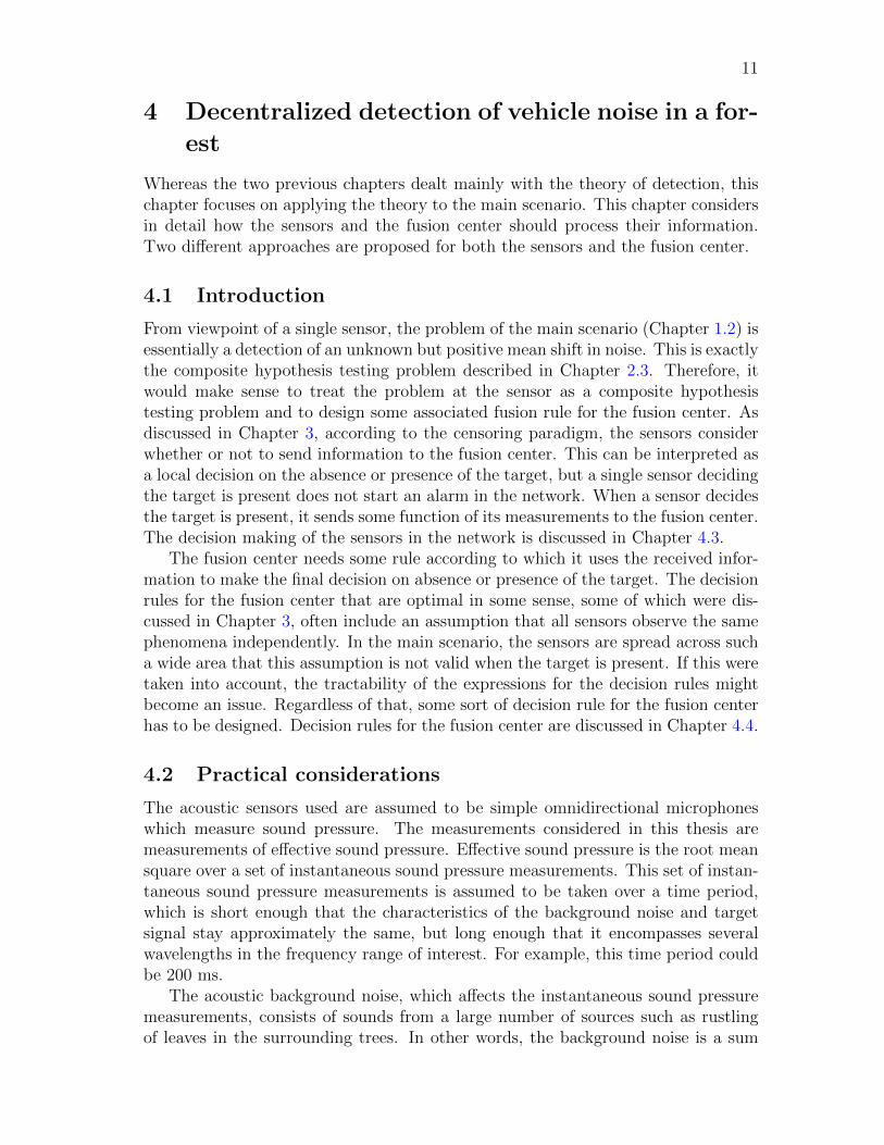
On the other hand, fixing the probability of false alarm to a value of PFA = 10−3,and varying the number of sensors N from 5 to 100 shows that the approximation isvalid also for other reasonable network sizes. The same probabilities of one sensoralarm (48) and multisensor alarms (49) of Figure 3 for different network sizes arepresented in Figure 4.

This shows equation (51) can be used to approximate the probability of falsealarm at the fusion center when γ0 is set to γ0 = 2 · Q−1(PFA). Same kind ofapproximation can be done when γ0 is set a little smaller. If the multiplier of

21

10 20 30 40 50 60 70 80 90 10010

−9

10−8

10−7

10−6

10−5

10−4

10−3

10−2

Network size

PFAat

thefusion

center

Pr {M ≥ 2}N ·Pr {yi(xi) > γ0}

Figure 4: Probabilities of different false alarm types at the fusion center as a functionof network size N with probability of false alarm of a single sensor set to PFA = 10−3.

Q−1(PFA) is in the range 1 . . . 2, the situation is still the same: a large value froma single sensor, or any values from two or more sensors will set off the alarm. Thedifference is that the large value from a single sensor does not have to be so large asbefore. Now the probability of noise causing one of the sensors to give such a largevalue that it sets off the alarm at the fusion center is given by

N · Pr {yi(xi) > γ0} = N ·Q(β ·Q−1(PFA)

), (55)

instead of equation (48). The probability of a single large value grows rapidly as themultiplier gets smaller than 2. For N = 20, PFA = 10−3, and multiplier, denoted byβ, in the range 1.3 . . . 1.7, the probabilities of the single large values are presentedin Figure 5. The probability that two or more sensors give false alarms at the sametime for the same values of N and PFA is 1.9 · 10−4, so the approximation holds, forthese values of N and PFA, fairly well when the multiplier is in the range 1.5 . . . 2.

Approximating the probability of false alarm at the fusion center when γ0 >2 ·Q−1(PFA) is more difficult. Restricting γ0 this way is not actually very confining,since the probability of false alarm of the fusion center can be set to any desiredvalue by adjusting the probability of false alarm of the sensors.

22

1.3 1.35 1.4 1.45 1.5 1.55 1.6 1.65 1.710

−6

10−5

10−4

10−3

Value of β

PFAat

thefusion

center

20 ·Pr

{yi(xi) > β ·Q−1(PFA)

}

Pr {M ≥ 2}

Figure 5: Probabilities of different false alarm types at the fusion center as a functionof β for network size N = 20 and PFA = 10−3.

4.5 Further considerations

In addition to the form of the tests at the sensors and the fusion center, there isa question of whether to set the thresholds of the sensors low and limit the falsealarms with a high fusion center threshold, or to set high sensor thresholds anda relatively low fusion center threshold. This is essentially a compromise betweenenergy consumption and performance. If the sensors did not censor anything, thefusion center would have the most information available, and it would be able tomake, at least in theory, the best decisions. However, this would quickly depletethe batteries of the sensors since they would have to send information in every timestep. If the sensor thresholds were set higher than the fusion center threshold, energyconsumption would be minimized, but performance would degrade and this wouldnot be a decentralized setting anymore. In this case, a single transmission froma single sensor would set off the alarm, and fusion center would not be needed atall. Since there is essentially no fusion center to combine the information in thiscase, because all the sensors use only their own measurements, performance of thesystem drops. The value of the threshold at the fusion center does not affect theenergy consumption of the network. It is a compromise between the probability offalse alarm and probability of detection or the delay in detection. Setting a high

23

threshold decreases both the probabilities of false alarm and detection, and viceversa, as discussed in Chapter 2.1.

In the previous chapters, each sensor is assumed to make a decision based on Kprevious measurements. The choice of K is a free design parameter. Taking severalprevious measurements into account each time step decreases the probability ofthe false alarms due to noise spikes, i.e., unusually large values of noise. If thenormality assumption of the background noise does not hold, the distribution of thenoise might be a long-tailed one, and noise spikes might be larger and more commonthan assumed. Choosing a K larger than one is especially useful in this situation.However, increasing K means averaging over more and more samples, which resultsin increasing delay in detection. The alarm at the fusion center will be set off afew time steps later than if there is no averaging. This is the price that is paid formitigating the effects of noise spikes.

24

5 Special characteristics of other scenarios

Characteristics of other scenarios akin to the main scenario of Chapter 1.2 are con-sidered in this chapter. Especially, the effects of these characteristics to detectionschemes in these scenarios are discussed here.

5.1 Detecting impulses

In the main scenario, the sensor network is trying to detect a vehicle in a forest. Thevehicle produces a continuous sound signal so taking measurements, e.g., once in asecond is adequate for detection. If the sound produced by the sound source is animpulse, the sensor might miss the impulse if it takes measurements too infrequently.For example, a gunshot is such a short sound that it can well be classified as animpulse [25, figure 1]. In such a scenario, the sound pressure must be monitored veryfrequently. It might be more practical to measure the sound pressure continuously,instead of taking measurements at certain intervals. The downside is that monitoringcontinuously depletes the batteries of the sensors faster, which reduces the lifetimeof the network. Also, in this type of impulse detection, averaging over severalmeasurements, i.e., choosing K larger than one, might not be a good idea. Averagingsmooths the signal, which is undesirable, as the objective is to detect abrupt impulsespikes.

5.2 Scenarios without a fusion center

As discussed in Chapter 4.5, letting a single sensor set off global alarm in the mainscenario results in inferior performance. Even if the sensors are deployed far awayfrom each other such that two sensors cannot detect the target at the same time, afusion center can be useful. Although only one sensor at a time can detect the target,it may be beneficial to have information at the fusion center from the other sensorssaying they do not detect any targets. Despite the sensors being quite distant fromeach other in this scenario, the sensors need to be within radio communication rangeof each other so that alarms can be transmitted across the network.

On the other hand, a detection system may be designed so that there is no needfor a designated fusion center. This is called fully decentralized detection. In thistype of system, sensors communicate between themselves to convey informationabout their measurements or local decision. The sensors try to find a consensusabout presence or absence of the target. When enough nodes agree on the targetbeing present, a global alarm is set off. Unlike a conventional decentralized system,a fully decentralized system is not vulnerable to fusion center breakdown. [26]

5.3 Direct communication with the fusion center

If the sensor setup is such that all sensors can communicate directly with the fusioncenter, there might not be need for large overheads in transmissions. In this case,the size of the transmissions may be heavily dependent on the quantization of the

25

information the sensors send to the fusion center. While in the main scenario using,for example, 3 bits instead of 10 bits to describe the information might not savemuch energy, as discussed in Chapter 3.1, in the direct communication setup itmight bring significant energy savings.

Additionally, if the sensors are arranged, e.g., into a linear or circular array withequal distances between the sensors, the system may give a good estimate on thedirection of the target [27]. For this the sensors have to be so close to each otherand the target has to be so close to the sensors that all sensors can hear the target.

5.4 Different types of sensors

Sensor types that can detect a target from as long distance as possible should beused for detection. However, other types of sensors may be more suitable for otherpurposes. E.g., it might make sense to deploy a few cameras to the network ofthe main scenario for classification purposes. These cameras could do automaticclassification of targets [28, 29] or send images of the detected targets out of thenetwork.

If the objective is to detect people, instead of vehicles, in a forest, infrared sensorsare a viable option [30]. Unlike acoustic sensors, infrared sensors require line of sightwith the target for detection. However, a single person walking in a forest mightnot make that much sound, so it is not obvious which sensor type would detect thetarget first. Especially in the case of heavy rain, the level of acoustic backgroundnoise can be so high that acoustic sensors might be practically useless in detectingpeople. It should also be taken into account that nearby thundering will cause allacoustic sensors to give alarms.

5.5 Target localization and tracking

In many scenarios, such as the main scenario, it is desirable to locate a target inaddition of detecting it. Some short-range sensors, such as cameras, may be betterthan acoustic sensors for localizing a target inside the network. Since they have ashort range, they cannot detect or localize a target that is at some distance from thenetwork. Thus, it is reasonable to do localization with acoustic or other long-rangesensors, too [31].

When localizing a target with acoustic or other long-range sensors, the detectionthresholds of the sensors should be lowered from the one used in detection mode.Many localization algorithms likely have better accuracy with more data, albeitsomewhat noise-corrupted data. It may not be of great importance anymore to saveenergy by reducing transmissions from the sensors when a target is detected. Instead,getting an accurate location estimate is far more important in many scenarios.

In addition to running only a localization algorithm, it is usually desirable run atracking algorithm on top of that. While localization algorithms typically consideronly the measurements from the current time instant, tracking algorithms can beused to exploit the time dependence between consecutive location estimates. In thetracking algorithms, the location estimate is based on prediction derived from the

26

previous estimates in addition to measurements. The statistical performance of therefined location estimates given by a tracking algorithm is generally better than thatof the raw location estimates given by the localization algorithm. Examples of thistype of tracking algorithms are the Kalman filter [20] and its extensions [32].

27

6 Simulations

A set of simulations was run in the main scenario and in an alternative scenario(see Chapter 6.7.3) to compare the performance of the two proposed schemes. Inaddition, the effect of different parameters of the schemes were studied. The simu-lations were run with Matlab R2010a software [21], which is a technical computingenvironment focusing on numerical computing. Simulation settings and results ofthe simulations are described in this chapter.

6.1 Simulation scenario

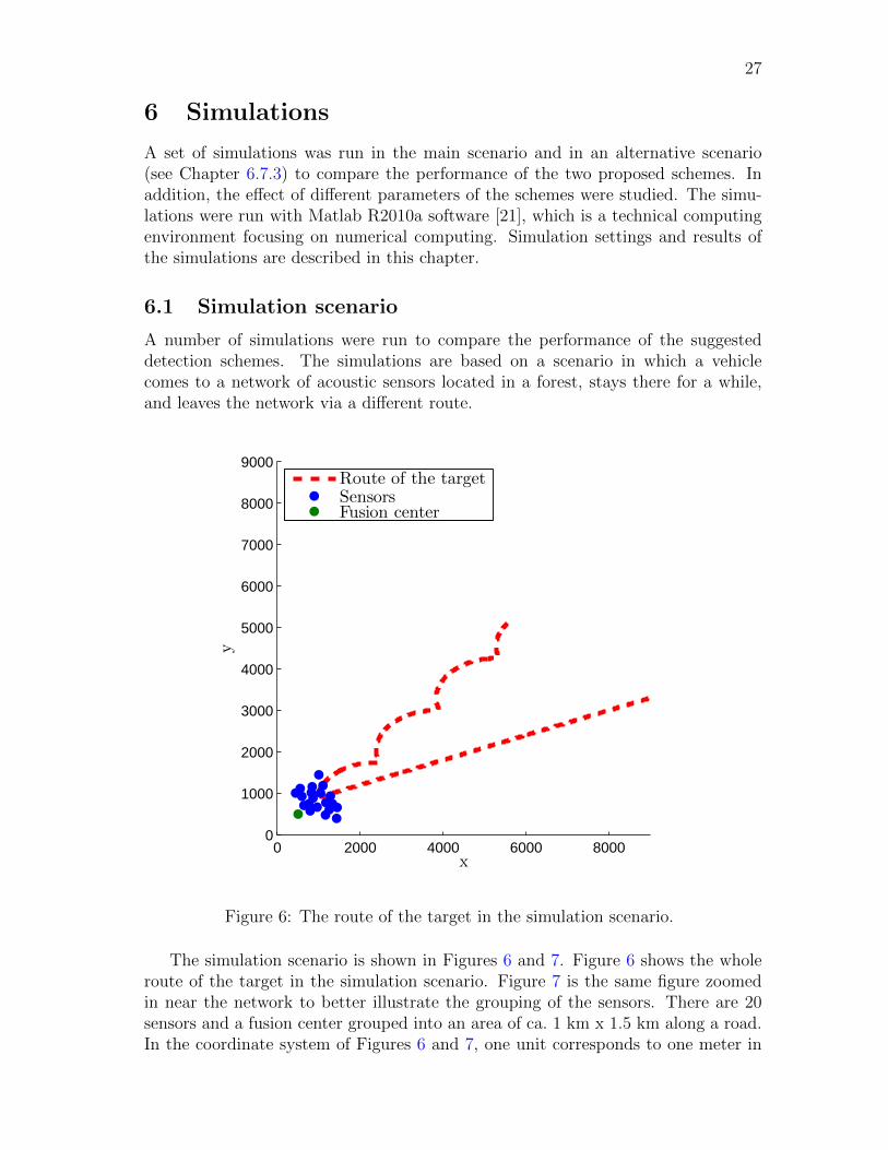
A number of simulations were run to compare the performance of the suggesteddetection schemes. The simulations are based on a scenario in which a vehiclecomes to a network of acoustic sensors located in a forest, stays there for a while,and leaves the network via a different route.

0 2000 4000 6000 80000

1000

2000

3000

4000

5000

6000

7000

8000

9000

x

y

Route of the targetSensorsFusion center

Figure 6: The route of the target in the simulation scenario.

The simulation scenario is shown in Figures 6 and 7. Figure 6 shows the wholeroute of the target in the simulation scenario. Figure 7 is the same figure zoomedin near the network to better illustrate the grouping of the sensors. There are 20sensors and a fusion center grouped into an area of ca. 1 km x 1.5 km along a road.In the coordinate system of Figures 6 and 7, one unit corresponds to one meter in

28

0 500 1000 1500 2000 25000

500

1000

1500

2000

2500

x

y

Route of the targetSensorsFusion center

Figure 7: The sensor network of the simulation scenario with the route of the targetnear the network.

the simulation. The locations of the sensors are marked with blue dots, the locationof the fusion center is marked with a green dot, and the route of the target is markedby the red curve. The target enters the network via the upper curve, stops for 1min 40 s in the place denoted by the red cross, and leaves the network via the lowercurve. The simulation lasts for 2000 seconds, i.e., approximately 34 min, and thespeed of the target as it moves is ca. 30 km/h.

6.2 Modeling sound propagation in a forest

A model for sound propagation in a forest is needed for the simulations. The modelused in the simulations is a simplified version of an ISO standard [36] describingsound propagation outdoors.

To calculate the sound pressure level at a sensor, the distance from the target andthe sound power level of the target are needed. In the ISO standard, the followingequation is given for the sound pressure level:

LfT (DW ) = LW +DC − A, (56)

where LfT (DW ) is the continuous downwind octave-band sound pressure level rela-tive to a 20 µPa reference sound pressure, LW is the sound power level of the sound

29

source relative to a 1 pW reference sound power, DC is the directivity correction indecibels, and A is the attenuation, in decibels, that occurs during propagation fromthe target to the sensor. For the simulation, it is assumed that the spectrum of thesound produced by the target is such that most of the energy is concentrated on anarrow frequency band so that only one octave band from LfT (DW ) can be takeninto account. In general, the attenuation of sound depends on frequency, so thisassumption makes the calculation of attenuation simpler. The target is assumed tobe an unidirectional sound source, so DC is set to DC = 0. Although the standardis defined for a sound propagating downwind, wind is not taken into account inthe simulations, and the same propagation model is used for sound propagating inall directions. Therefore, the sound pressure level at a sensor due to the target issimplified into

LP = LW − A. (57)

The attenuation A is divided into components in the standard:

A = Adiv + Aatm + Agr + Abar + Amisc, (58)

where Adiv is the attenuation due to geometrical divergence, Aatm is the attenuationdue to atmospheric absorption, Agr is the attenuation due to the ground effect, Abaris the attenuation due to a barrier, and Amisc is the attenuation due to miscellaneousother effects.

Besides the forest, no other obstacles between a sensor and the target are takeninto account, so Abar = 0. The miscellaneous other factors are also assumed to bezero, i.e., Amisc = 0.

Since the objective is to detect a vehicle in the simulation, most of the energyof the sound is assumed to be around the frequency of 100 Hz [37, 38]. This ap-proximation might not be valid with all vehicles, but it is deemed an appropriatesimplification. With this assumption, the atmospheric absorption and ground effectcan be calculated for the frequency of 100 Hz, and their frequency dependence canbe neglected.

In the standard atmospheric absorption is calculated as

Aatm = αsd/1000, (59)

where αs is a parameter depending on the frequency of the sound, and d is thedistance the sound propagates in the air. For frequencies around 100 Hz, αs isapproximately 0.2, so for, e.g., the distance of 1 km, Aatm = 0.2 dB. This is such asmall value that it is lost under the other inaccuracies of the model. Thus, in thesimulation, the atmospheric absorption is set to Aatm = 0.

For the geometric divergence, there is an equation in the standard that is directlyapplied in the simulation:

Adiv = 20 log10

(d

d0

)+ 11, (60)

where d is the distance the sound propagates, and d0 is the reference distanced0 = 1 m. The constant 11 in the equation relates the sound power level of an

30

omnidirectional sound source to the sound pressure level at a distance of 1 m [39,p. 88].

Several different methods for calculating the attenuation due to ground effect aregiven in the standard. In addition of frequency, the ground effect depends on theheight of the sensors and the target. However, based on actual measurements in aFinnish forest [40, figure 3 (left)], the attenuation due to ground effect in simulationsis set to Agr = 8 dB.

As a summary, the sound pressure level LP [dB] at a sensor due to the target iscalculated from the sound power level of the target, and its distance from the sensoras

LP = LW − A = LW − (Adiv + Agr) = LW − 20 log10(d)− 19. (61)

6.3 Wireless communication model

Usually the research on decentralized detection and the related simulations do notconsider the communication aspect of the sensor network. As discussed in Chapter1.1, the sensors are typically connected by a wireless communication channel. Tomake the simulations more realistic, a model for the communication between sensorsis implemented in the simulations. The fundamental function of this model in thesimulations is discarding some of the information sent from the sensors to the fusioncenter.

There are essentially two major reasons why the measurement information fromsensors might not received by the fusion center:

� In the physical layer, there may be so low a signal-to-noise ratio (SNR) thatthe receiving sensor or fusion center cannot properly decode the informationfrom a transmission.

� In the medium access control (MAC) layer, there may be congestion in thetransmission medium.

Both of these are taken into account in the model for wireless communication in thenetwork. Since the lifetime of the battery-powered sensors depend on energy con-sumption, energy-efficiency is of paramount importance in sensor networks. Energycan be saved by limiting the transmit power of the sensors, which results in quite alow SNR at the receiver. Thus, a relatively high percentage of the information sentby the sensors may be lost because of this. Sleep cycles [34] may also be utilizedby the sensors to save energy. During sleep periods, a sensor’s radio is completelyturned off, so it cannot transmit or receive anything during that period. The activeperiods, when the radio is actually on, may be short, and there may be a lot oftraffic in the network during these periods. The information from all the sensorsmay not make it to the fusion center during an active period in case of congestionin the network.

To represent the loss of detection information from low SNR, a simple approachis applied. Each value a sensor sends to the fusion center is lost with some proba-bility PSNR. This is a baseline for the probability of packet loss, where one packet

31

constitutes one value a sensors sends. In the simulations, it is assumed the sensorsare set to transmit at quite a low power and, thus, the value for PSNR is set quitehigh, PSNR = 0.02. This means that 2% of packets are lost regardless of the trafficintensity at MAC layer.

To model the packet loss resulting from congestion in the network, a methodfrom article [35] is used. A contention-based MAC scheme is considered where thesensors, which have a packet to send, compete for the used of the communicationchannel. The active period, discussed above, is split into S time slots for analysis.Denote the number of sensors, which have a packet to send, as B. At each time slot,each of the B sensors transmit with probability p. If two or more sensors try to sendduring the same time slot, all their transmissions fail, and they have to try againat later time slots. A packet is lost if it is not successfully transmitted during theactive period, i.e., during the S time slots. According to [35], the probability thata packet is lost due to congestion in the communication channel, for each packetindividually, can be approximated by

Pr {packet lost} =((1− p) + p(1− (1− p)B−1)

)S. (62)

The optimal value for p under the assumptions in [35] is approximately

popt ≈2

B + 2. (63)

However, the sensors do not know the number of sensors that have something tosend, B. In the simulations, sensors assume the worst-case scenario and use thenumber of sensors in the network, N , instead of B, in equation (63). The numberof time slots, S, used in simulations is S = 100. The shape of function (62) withS = 100, network size N = 20, and p = 2

N+2= 2

20+2= 1

11is shown in Figure 8.

This approach to modeling the nonideal communication between sensors is actu-ally appropriate only for sensors communicating directly with the fusion center, andthe networking aspect, different transmit power levels, different number of hops ofdifferent packets in the network, or different distances between the sensors are notmodeled. A more elaborate scheme would have to be devised to account for these.This simple model used in simulations is justified by that fact that the primaryinterest is on the percentage of lost packets. It is not relevant, which packets aredropped and which are received.

6.4 Default settings for the simulation

A sound power level for the target was set from [4, figure 4]. The value chosen forthe sound power level is 115 dB which corresponds to a sound pressure level of 104dB at a distance of 1 m according to the rule of thumb [39]

LP1m [dB relative to 20 µPa] = LW [dB relative to 1 pW]− 11, (64)

where LP1m denotes the sound pressure level at a distance of 1 m from the source,and LW denotes the sound power level of the source.

32

0 5 10 15 200

0.05

0.1

0.15

0.2

0.25

Number of sensors having a packet to send, B

Pr{p

acketlost}

Figure 8: Probability of packet loss for a single packet as a function of the numberof sensors having something to send for the settings of simulation scenario describedin Chapter 6.1.

The acoustic background noise is modeled by a normal distribution, see Chapter4.2. Therefore, two parameters have to be set for the noise, mean and variance. Themean was set to 1.1 mPa, which corresponds to a sound pressure level of 35 dB, andthe variance was set to 10−7 Pa2. It is assumed the sensors have very good estimatesof the mean and the variance of the background noise, i.e., the estimation errors areignored, and the sensors use the true values instead.

All sensors were set to the same level of probability of false alarm in the simula-tions. For the combining standard deviations scheme, the probability of false alarmfor the fusion center is fully determined by the false alarm rate of the sensors. Mul-tiplier of the fusion center threshold for the combining standard deviations scheme,β, is set to its default value of two. For a desired level of PFA at the fusion center,the PFA of the sensors was searched by iteration from function (52).

For the maximum likelihood scheme, the thresholds for the sensors and the fusioncenter were searched by iteration with the Matlab script of Appendix A. First,the threshold for the sensors, ρ, was set to yield approximately the same PFA atthe sensors as in the combining standard deviations scheme. After ρ was set, thethreshold for the fusion center, α, was searched which yields approximately thedesired PFA.

33

K is set to one for all sensors, i.e., sensors use only their current measurementat each time instant in their decision-making. The sensors take measurements andrun their detection algorithm at intervals of one second. The fusion center alsomakes a decision of presence or absence of the target once in a second. Some of thesettings presented here or in Chapter 6.1 are changed in some of the simulations.The changes are discussed in the chapters discussing results for the correspondingsimulation.

6.5 Simulation 1 — Performance at different rates of PFA

In this simulation, the detection performance of the combining standard deviationsscheme and the maximum likelihood scheme is compared. As described in Chapter6.4, in both schemes the sensors were set to the same level of PFA, and the samelevel of PFA was set to the fusion center. The simulation was run with three differentrates of PFA at the fusion center, 10−4, 10−5, and 10−6. These rates were chosensince they represent a reasonable compromise between number of false alarms anddetection sensitivity for the main scenario. The detection thresholds correspondingto these rates in both schemes are listed in Table 2.

Table 2: Settings of the fusion center and the sensors in simulation 1.

Setting number 1 2 3

PFA of fusion center 10−4 10−5 10−6

PFA of sensors 7.29 · 10−4 2.30 · 10−4 7.27 · 10−5

ρ 301 878 2640α 117 295 900

A thousand simulations were run with each false alarm rate for both schemes.The average number alarms was computed from the results for each false alarmrate and for both schemes. A larger number of alarms is considered to be better,although there probably are false alarms included in these alarms. However, theseare ignored for two reasons:

� Most of the alarms are actual detections of the target.

� Simulations are run to compare the relative performance of the two schemes,and the fusion center is set to the same PFA for both schemes. The expectednumber of false alarms is same for both schemes. Thus, the false alarms donot play a large role in comparison of the two schemes.

The results of this simulation are shown in Figure 9. In all three levels of PFA,the combining standard deviations scheme performs significantly better than themaximum likelihood scheme. Although the maximum likelihood scheme is semi-optimal in a more ideal scenario, i.e., where all the sensors are at an equal distance

34

0

100

200

300

400

500

600

700

Probability of false alarm of the fusion center

Number

ofalarms

10−4 10−5 10−6

Combining standard deviationsMaximum likelihood

Figure 9: Number of alarms in the simulation scenario for three different rates ofPFA for both detection schemes.

from the target, its performance is not good in this type of more practical scenario.This shows it is not robust against deviations from assumptions since it performsclearly worse than an heuristic scheme without optimality properties.

6.6 Simulation 2 — Different noise distribution

The sensors assume in their detection algorithms that the background acoustic noiseis normal distributed. In this simulation, the performance of the proposed schemesis studied if this assumption does not hold. The background noise in this simulationis gamma distributed [41] with the same expected value and variance as the normaldistributed noise in simulation 1, i.e., expected value µ = 1.1 mPa and varianceσ2 = 10−7 Pa2. The gamma distribution has two parameters, shape parameterkG > 0, and scale parameter θG > 0. Its expected value equals kGθG, and its varianceequals kGθ

2G. Setting the same expected value and variance for the background noise

as in simulation 1 means setting kG and θG such that

{kGθG = µkGθ

2G = σ2.

(65)

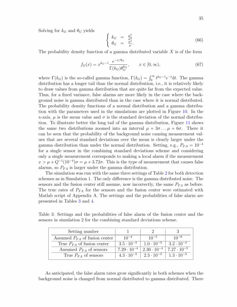
35

Solving for kG and θG yields {kG = µ2

σ2

θG = σ2

µ.

(66)

The probability density function of a gamma distributed variable X is of the form

fG(x) = xkG−1 e−x/θG

Γ(kG)θkGG, x ∈ [0,∞), (67)

where Γ(kG) is the so-called gamma function, Γ(kG) =∫∞

0tkG−1e−tdt. The gamma

distribution has a longer tail than the normal distribution, i.e., it is relatively likelyto draw values from gamma distribution that are quite far from the expected value.Thus, for a fixed variance, false alarms are more likely in the case where the back-ground noise is gamma distributed than in the case where it is normal distributed.The probability density functions of a normal distribution and a gamma distribu-tion with the parameters used in the simulations are plotted in Figure 10. In thex-axis, µ is the mean value and σ is the standard deviation of the normal distribu-tion. To illustrate better the long tail of the gamma distribution, Figure 11 showsthe same two distributions zoomed into an interval µ + 3σ . . . µ + 6σ. There itcan be seen that the probability of the background noise causing measurement val-ues that are several standard deviations over the mean is clearly larger under thegamma distribution than under the normal distribution. Setting, e.g., PFA = 10−4

for a single sensor in the combining standard deviations scheme and consideringonly a single measurement corresponds to making a local alarm if the measurementx > µ+Q−1(10−4)σ = µ+ 3.72σ. This is the type of measurement that causes falsealarms, so PFA is larger under the gamma distribution.

The simulation was run with the same three settings of Table 2 for both detectionschemes as in Simulation 1. The only difference is the gamma distributed noise. Thesensors and the fusion center still assume, now incorrectly, the same PFA as before.The true rates of PFA for the sensors and the fusion center were estimated withMatlab script of Appendix A. The settings and the probabilities of false alarm arepresented in Tables 3 and 4.

Table 3: Settings and the probabilities of false alarm of the fusion center and thesensors in simulation 2 for the combining standard deviations scheme.

Setting number 1 2 3

Assumed PFA of fusion center 10−4 10−5 10−6

True PFA of fusion center 3.5 · 10−3 1.0 · 10−3 3.2 · 10−4

Assumed PFA of sensors 7.29 · 10−4 2.30 · 10−4 7.27 · 10−5

True PFA of sensors 4.3 · 10−3 2.3 · 10−3 1.3 · 10−3

As anticipated, the false alarm rates grow significantly in both schemes when thebackground noise is changed from normal distributed to gamma distributed. There

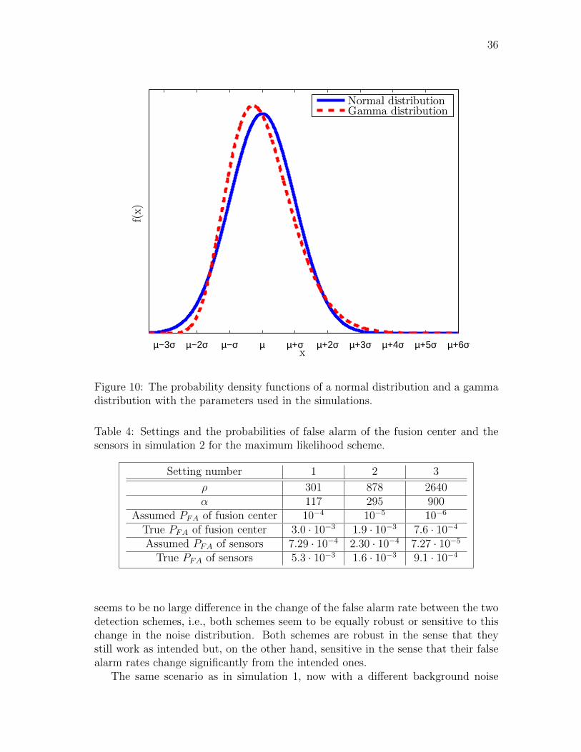
36

x

f(x)

µ−3σ µ−2σ µ−σ µ µ+σ µ+2σ µ+3σ µ+4σ µ+5σ µ+6σ

Normal distributionGamma distribution

Figure 10: The probability density functions of a normal distribution and a gammadistribution with the parameters used in the simulations.

Table 4: Settings and the probabilities of false alarm of the fusion center and thesensors in simulation 2 for the maximum likelihood scheme.

Setting number 1 2 3

ρ 301 878 2640α 117 295 900

Assumed PFA of fusion center 10−4 10−5 10−6

True PFA of fusion center 3.0 · 10−3 1.9 · 10−3 7.6 · 10−4

Assumed PFA of sensors 7.29 · 10−4 2.30 · 10−4 7.27 · 10−5

True PFA of sensors 5.3 · 10−3 1.6 · 10−3 9.1 · 10−4

seems to be no large difference in the change of the false alarm rate between the twodetection schemes, i.e., both schemes seem to be equally robust or sensitive to thischange in the noise distribution. Both schemes are robust in the sense that theystill work as intended but, on the other hand, sensitive in the sense that their falsealarm rates change significantly from the intended ones.

The same scenario as in simulation 1, now with a different background noise

37

x

f(x)

µ+3σ µ+4σ µ+5σ µ+6σ

Normal distributionGamma distribution

Figure 11: The probability density functions of a normal distribution and a gammadistribution with the parameters used in the simulations in an interval µ+3σ . . . µ+6σ.

distribution, was run a thousand times for each setting for both schemes, and theaverage number of alarms in each case was computed. The results of simulation2 are shown in Figure 12. Although there are more false alarms now, the vastmajority of the alarms are still valid detections of the target. Therefore, detectionperformance can be compared by looking at the total number of alarms. It canbe seen by comparing Figures 9 and 12 that the number of alarms went up forall settings in both detection schemes as the background noise distribution waschanged to a gamma distribution. Also, as can be seen from Tables 3 and 4, theprobability of false alarm increased because of the long tail of the noise distribution.There is essentially no change in the relative performance of the two schemes withthe corresponding settings. Thus, changing the background noise distribution fromnormal to gamma distribution resembles the situation of decreasing the thresholdsin order to have a larger probability of detection at the cost of having a larger PFA.However, ratio of the number of alarms and PFA is worse in the case of gammadistributed noise. This means that detecting the target in gamma distributed noiseis a more difficult problem than detecting it in normal distributed noise.

38

1 2 30

100

200

300

400

500

600

700

800

Setting number

Number

ofalarms

Combining standard deviationsMaximum likelihood

Figure 12: Number of alarms in simulation 2 for three different settings for bothdetection schemes.

6.7 Simulation 3 — Binary sensors

6.7.1 Introduction

Quantization of the data the sensors send to the fusion center is discussed in Chapter3.1. It is argued there that the energy savings achieved by quantizing the measure-ments are likely to be minor. In this simulation, the performance of the combiningstandard deviations scheme is studied in the situation, where the sensors quantifytheir measurements to a single bit, i.e., the sensors give only a local yes/no decisionof presence of the target.

Consider the combining standard deviations scheme without quantization. Asexplained in Chapter 4.4.2, the probability of a single sensor giving a large enoughvalue to set off the fusion center threshold by itself is negligibly small. Also, twosensors making a local decision the target is present and giving any value alwayssets off the alarm. Therefore, if a scheme with extreme quantization, i.e., binarysensors, is considered, setting the fusion center to decide the target is present whentwo sensors give an alarm yields approximately the same PFA at the fusion center.Thus, the two situations can be compared and the effect of binary sensors on thedetection performance can be seen. Although the PFA at the fusion center is thesame in both situations, the detecion performance is expected to be worse with

39

binary sensors. This stems from the fact that a single sensor cannot produce a largevalue which would set off the alarm at the fusion center, even if the target were rightnext to the sensor.

6.7.2 Main scenario

The main scenario, described in Chapter 6.1, was run with both the basic combiningstandard deviations scheme and binary sensors. In both cases, PFA of the fusioncenter was set to 10−4. In case of the binary sensors, the fusion center sets off thealarm when it recieves local alarms from at least two sensors.

For both setups, the simulation was run a thousand times, and the averagenumber of alarms in the basic combining standard deviations scheme was 698.2,and in the binary sensors setup, the average number of alarms was 698.2. In bothsetups, the performance is the same within rounding error. This is due to thenetwork topology in the main scenario. The sensors are grouped so close to eachother that many sensors detect the approaching target almost at the same time.When one sensor has so strong a signal from the target that it would cause thefusion center to set off the alarm by itself, the measurement of at least one other hasrisen above its detection threshold, and it sends a local alarm to the fusion center,too.

6.7.3 Linear array

To illustrate the possible degredation of detection performance when the sensorsgive binary information instead of more accurate information to the fusion center,another simulation scenario is considered. In this scenario, there are only 5 sensors,and they are grouped to a linear equidistant array. The distance between sensorsis 400 m, whereas in the main scenario the distance is ca. 200 m. The sensors aregrouped along the y-axis of the coordinate system and the target approaches alongthe y-axis as well. The speed of the target is ca. 30 km/h and it moves 8 km duringthe simulation. This scenario is illustrated in Figure 13.

The sensitivity of the network is set to the same level as in the binary sensorsimulation of the main scenario, i.e., PFA of the fusion center is set to 10−4. Asshown in Table 2, setting PFA of the sensors to 7.29 · 10−4 results in PFA of 10−4

at the fusion center in the main scenario. Now the network has a different size, N ,so according to equation (52), a different sensitivity has to be set to the sensors toget the desired PFA of 10−4 at the fusion center. By iteration, it was found thatsetting the sensors to PFA = 3.18 · 10−3 yields approximately PFA = 10−4 at thefusion center.

This simulation was run one thousand times with both basic and binary sensorsin the combining standard deviations scheme. The average number of alarms in thebasic combining standard deviations scheme was 270.4, and in the binary sensorssetup, the average number of alarms was 268.0. Unlike in the main scenario withbinary sensors, discussed in Chapter 6.7.2, now there is a notable difference in thenumber of alarms between the basic and the binary setup. This difference wouldlikely grow larger if the distance between sensors were increased. On the other hand,

40

0 200 400 600 800 10000

1000

2000

3000

4000

5000

6000

7000

8000

9000

x

y

Route of the target

Sensors

Fusion center

Figure 13: Sensor setup and the route of the target in simulation 3b: linear array.

the difference would likely become smaller if the target approached from some otherdirection. This scenario, where the target approaches from the same direction alongwhich the sensors are grouped, is essentially a worst-case scenario from the viewpointof the detection performance of the binary sensors setup.

6.8 Simulation 4 — Effect of β

6.8.1 Introduction

As discussed in Chapter 4.4.2, the fusion center threshold parameter, β, of thecombining standard deviations scheme can be adjusted a little lower than its defaultvalue of 2. Adjusting beta this way allows a single sensor to set off easier the globalalarm at the fusion center. If β is adjusted by a sufficiently small amount, this canbe done with a very small increase in the PFA of the fusion center. In this simulation,the effect of β on the detection performance of the combining standard deviationsscheme is studied.

6.8.2 Main scenario

The main scenario was run with the combining standard deviations scheme andwith two different values of β. In both cases, PFA of the fusion center was set to

41

approximately 10−4. The default value of β is 2, so this is the baseline for comparisonwith a lower value of β. An increase in PFA that is two orders of magnitude smallerthan PFA was deemed a negligible change. According to equation (55), settingβ = 1.67 in the main scenario increases PFA by 1.06 · 10−6, so β = 1.67 was used asthe lower value.

For both settings, the simulation was run a thousand times, and the averagenumber of alarms was computed. With β = 2, the average number of alarms was698.2 and with β = 1.67, the average number of alarms was 698.5. The increase inthe number of alarms is very small and may be caused only by the tiny increase inthe number of false alarms. This is the same result as in the simulation with binarysensors, described in Chapter 6.7.2, and the reasons are the same, too. The sensorsare grouped relatively close to each other, and the target approaches from such adirection, that the measurement of the sensor closest to the target does not havethe time to rise to a level in which it would set off the alarm of the fusion centerby itself, even though the threshold is now lower. Other nearby sensors give theiralarms before that happens and, thus, a lower value of β does not help here.

6.8.3 Linear array

To show that decreasing β might be beneficial in some cases, the linear array scenariowith 5 sensors, described in Chapter 6.7.3, was run with the same PFA of the fusioncenter and two different values of β, the default value of 2 and a lower value. Nowthere is a different number of sensors and a different PFA of the sensors, so a newvalue for β has to be found. According to equation (55), setting β = 1.85 increasesPFA by 1.12 · 10−6, so β = 1.85 was used as the lower value.

As before, for both settings, the simulation was run one thousand times, andthe average number of alarms was computed. The results are shown in Figure 14,and parameters for the different settings are summarized in Table 5. With β = 2,the average number of alarms was 270.4 and with β = 1.85, the average number ofalarms was 271.8. Now there is a tangible difference in the detection performancebetween the setups with different values of β. This goes to show that detectionperformance can be improved in some cases by adjusting β slightly lower than itsdefault value of 2.

Table 5: Summary of the parameters for the different settings in the linear arrayscenario.

Setting β Sensor PFA Approximate fusion center PFA

Basic 2 3.18 · 10−3 10−4

Alternative 1 1.85 3.18 · 10−3 10−4 + 10−6

Alternative 2 2 3.19 · 10−3 10−4 + 10−6

The increase in the number of alarms by adjusting β in this scenario is largerthan the one achieved by directly increasing PFA of the sensors. To show this, a

42

Basic Alternative 1 Alternative 2269

269.5

270

270.5

271

271.5

272

272.5

273

Settings

Number

ofalarms

Figure 14: Average number of alarms from a thousand simulation runs in the lineararray scenario with 5 sensors using three different settings in the combining standarddeviations scheme.

batch of simulations was run where the PFA of the fusion center was increased byapproximately the same amount as decreasing β to 1.85 yielded. As stated above,setting β = 1.85 increases PFA by 1.12 ·10−6. According to equation (52), increasingPFA of the sensors from 3.18·10−3 to 3.19·10−3 increases the PFA of the fusion centerby approximately 1.11 · 10−6. A simulation was run one thousand times with β = 2and PFA = 3.19 · 10−3. The result of the simulation is shown in Figure 14 and theparameters discussed above are listed in Table 5. The average number of alarms was270.5, which is smaller than the number of alarms obtained by setting β = 1.85, eventhough the increase in PFA is the same. This shows that, in some cases, adjustingβ is results in a better detection performance than directly adjusting the PFA of thesensors. However, β can be adjusted only by a little. For larger modifications to thesensitivity of the sensors, their PFA has to be adjusted directly.

6.9 Discussion of simulation results

Results of the simulations conducted in Simulink indicate that the combining stan-dard deviations scheme performs better in the main scenario. Simulations also showthat the proposed schemes work appropriately under a long tailed background noise

43

distribution. Although performance decreases for both schemes, it still remains atan acceptable level. The difference in the performance of the two schemes is ap-proximately the same under the long tailed noise distribution, i.e., the combiningstandard deviations scheme still performs considerably better than the maximumlikelihood scheme.

It is quite surprising that the heuristic combining standard deviations schemeworks so much better in the main scenario than the maximum likelihood scheme,which semi-optimal in a more idealistic scenario. The motivation for developing thecombining standard deviations scheme was to devise a somewhat simpler schemewith easier setup of parameters. In addition these benefits, performance in themain scenario is significantly better than that of the maximum likelihood scheme.Also, the combining standard deviations scheme is equally robust against a longtailed noise distribution as the maximum likelihood scheme.

44

7 Conclusions and future work

A summary of the thesis is given is this chapter. Also, usefulness of the schemes arediscussed here, and suggestions are given for future research.

7.1 Conclusions

Decentralized detection is an area of research which focuses on detection of targetswith a network of sensors. The research conducted in this area often concentrateson theoretical issues and ideal situations, whereas this thesis discusses the problemsin a realistic scenario. The main scenario of this thesis is detecting a vehicle in aforest using acoustic sensors.

The main problem with many of the detection schemes developed for ideal sce-narios is the requirement that all sensors observe the exactly same phenomena. Thefact that the target is at a different distance from the sensors is typically not takeninto account. Another assumption, which is often made, is the assumption of nor-mal distributed background noise. In the derivations of the detection schemes ofthis thesis, the same assumption is made, but one of the simulations is conductedwith another noise distribution. This thesis studies the performance of two schemesin the aforementioned main scenario. One of the schemes is the maximum likelihoodscheme which has some optimality properties under certain assumptions. The otherone is a heuristic scheme named combining standard deviations, based on classicaldetection theory, with no optimality properties.

The combining standard deviations scheme offers easier setup of threshold val-ues and the approximation of false alarm rates for given thresholds using simpleequations. Based on simulation results, it also seems to offer better performance.The main objective of this thesis was to find a practically viable detection schemefor the realistic main scenario. While both presented schemes can be used for thisscenario, the combining standard deviations scheme offers better performance andeasier setup in the type of scenario considered here.

7.2 Directions of future work

Neither scheme properly utilizes information from sensors, which send nothing, andthe geometry of the network. Consider a situation in which sensors are placed sodensely that their detection regions overlap, and only a sensor in the center of thenetwork gives a local alarm. This alarm is almost certainly a false alarm since noneof the other sensors nearby detect anything. On the other hand, if a sensor inthe edge of the network gives a local alarm, and none of the nearby sensors detectanything, it is much more likely to be real detection of a target approaching thenetwork. The fusion center does not use this information any way in its decisionrule. A viable direction for future work could be to try to find a way to use thisinformation in the decision rule of the fusion center.

Another natural step would be to use actual measurements as the acoustic back-ground noise in simulations, or better yet, employ a network of sensors in a forest,

45

and conduct a live experiment. It would be of interest to try different detectionschemes in different background noise conditions, for example, in a windy or rainyenvironment. To realistically assess the performance in these type of conditions, theanalysis would have to be based on actual measurements in the desired conditions.

46

References

[1] Akyildiz, I. F., Su, W., Sankarasubramaniam, Y. and Cayirci, E. Wireless Sen-sor Networks: A Survey. Computer Networks, March 2002, vol. 38, no. 4, pp.393–422.

[2] Viswanathan, R. and Varshney, P. K. Distributed Detection with Multiple Sen-sors: Part 1 — Fundamentals. Proceedings the IEEE, January 1997, vol. 85,no. 1, pp. 54–63.

[3] Arampatzis, T., Lygeros, J. and Manesis, S. A Survey of Applications of Wire-less Sensors and Wireless Sensor Networks. Proceedings of the 2005 IEEE In-ternational Symposium on Intelligent Control, 2005, Mediterrean Conferenceon Control and Automation, 2005, pp. 719–724.

[4] Becker, G. and Gudesen, A. Passive Sensing with Acoustics on the Battlefield.Applied Acoustics, 2000, vol. 59, no. 2, pp. 149–178.

[5] Kay, S. M. Fundamentals of Statistical Signal Processing, Volume II: DetectionTheory. New Jersey, Prentice Hall PTR, 1998.

[6] Neyman, J. and Pearson, E. S. On the Problem of the Most Efficient Testsof Statistical Hypotheses. Philosophical Transactions of the Royal Society ofLondon. Series A, Containing Papers of a Mathematical or Physical Character,1933, vol. 231, pp. 289–337.

[7] Chamberland, J.-F. and Veeravalli, V. V. Wireless Sensors in Distributed De-tection Applications — An Alternative Framework Tailored to DecentralizedDetection. IEEE Signal Processing Magazine, May 2007, vol. 24, no. 3, pp.16–25.

[8] Appadwedula, S., Veeravalli, V. V. and Jones, D. L. Decentralized Detectionwith Censoring Sensors. IEEE Transactions on Signal Processing, April 2008,vol. 56, no. 4, pp. 1362–1373.

[9] Warren, D. and Willett, P. Optimal Decentralized Detection for ConditionallyIndependent Sensors. Proceedings of the 1989 American Control Conference,June 1989, pp. 1326–1329.

[10] IEEE 802.11. Wireless LAN Medium Access Control (MAC) and Physical Layer(PHY) Specifications. 2007 revision. New York, IEEE Standards Association.1184 p.

[11] IEEE 802.15.1. Wireless Medium Access Control (MAC) and Physical Layer(PHY) Specifications for Wireless Personal Area Networks (WPANs). NewYork, IEEE Standards Association, 2005. 580 p.

47

[12] Cho, S. and Chandrakasan, A. P. Energy Efficient Protocols for Low DutyCycle Wireless Microsensor Networks. ICASSP Proceedings 2001, vol. 4, SaltLake City, Utah, pp. 2041–2044.

[13] Appadwedula, S. Energy-efficient Sensor Networks for Detection Applications.Ph.D. Thesis. University of Illinois, USA, 2003.

[14] Tsitsiklis, J. N. and Athans, M. On the Complexity of Decentralized DecisionMaking and Detection Problems. IEEE Transactions on Automatic Control,May 1985, vol. 30, no. 4, pp. 440–446.

[15] Yan, Q. and Blum, R. S. On Some Unresolved Issues in Finding OptimumDistributed Detection Schemes. IEEE Transactions on Signal Processing, De-cember 2000, vol. 48, no. 12, pp. 3280–3288.

[16] Tenney, R. R. and Sandell, N. R., Jr. Detection with Distributed Sensors. IEEETransactions on Aerospace and Electronic Systems, July 1981, vol. 17, no. 4,pp. 501–510.

[17] Rago, C., Willett, P. and Bar-Shalom, Y. Censoring Sensors: A Low-Communication-Rate Scheme for Distributed Detection. IEEE Transactions onAerospace and Electronic Systems, April 1996, vol. 32, no. 2, pp. 554–568.

[18] Le Cam, L. The Central Limit Theorem Around 1935. Statistical Science, 1986,vol. 1, no. 1, pp. 78–91.

[19] Quach, A. and Lo, K. Automatic Target Detection Using a Ground-based Pas-sive Acoustic Sensor. IEEE Proceedings of Information, Decision and Control,1999, Pyrmont, Australia, pp. 187–192.

[20] Kay, S. M. Fundamentals of Statistical Signal Processing: Estimation Theory.New Jersey, Prentice Hall PTR, 1993.

[21] Matlab website, July 2011, http://www.mathworks.com/products/matlab/

[22] Tse, D. and Viswanath, P. Fundamentals of Wireless Communication, Cam-bridge University Press, 2005.

[23] Adams, R. A. Calculus: A Complete Course. 6th ed. Toronto, Pearson Educa-tion Canada Inc., 2006.

[24] Springer, M. D. and Thompson, W. E. The Distribution of Products of Inde-pendent Random Variables. SIAM Journal on Applied Mathematics, May 1966,vol. 14, no. 3, pp. 511–526.

[25] Chacon-Rodriguez, A., Julian, P., Castro, L., Alvarado, P. and Hernandez, N.Evaluation of Gunshot Detection Algorithms. IEEE Transactions on Circuitsand Systems — I: Regular Papers, February 2011, vol. 58, no. 2, pp. 363–373.

48

[26] Nyberg, T. Fully Decentralized Sequential Detection in an Underwater Setting.M.Sc. Thesis. Stockholm University, Sweden, 2008.

[27] Krim, H. and Viberg, M. Two Decades of Array Signal Processing Research:The Parametric Approach. IEEE Signal Processing Magazine, July 1996, vol.13, no. 4, pp. 67–94.

[28] Gupte, S., Masoud, O., Martin, R. F. K. and Papaniikolopoulos, N. P. Detectionand Classification of Vehicles. IEEE Transactions on Intelligent TransportationSystems, March 2002, vol. 3, no. 1, pp. 37–47.

[29] Lipton, A. J., Fujiyoshi, H. and Patil, R. S. Moving Target Classification andTracking from Real-Time Video. Fourth IEEE Workshop on Applications ofComputer Vision, WACV ’98, Proceedings, October 1998, pp. 8–14.

[30] Bertozzi, M., Broggi, A., Caraffi, C., Del Rose, M., Felisa, M. and Vezzoni, G.Pedestrian Detection by Mean of Far-Infrared Stereo Vision. Computer Visionand Image Understanding Journal, May 2007, vol. 106, no. 2–3, pp. 194–204.

[31] Sheng, X. and Hu, Y.-H. Maximum Likelihood Multiple-Source LocalizationUsing Acoustic Energy Measurements with Wireless Sensor Networks. IEEETransactions on Signal Processing, 2005, vol. 53, no. 1, pp. 44–53.

[32] Ristic, B., Arulampalam, S. and Gordon, N. Beyond the Kalman Filter —Particle Filters for Tracking Applications. Artech House, 2004.

[33] Simulink website, December 2011,http://www.mathworks.se/products/simulink/

[34] Hsin, C.-f., Liu, M. Network Coverage Using Low Duty-cycled Sensors: Ran-dom & Coordinated Sleep Algorithms. ISPN ’04: Proceedings of the 3rd Inter-national Symposium on Information Processing in Sensor Networks, 2004, pp.433–442.

[35] Rabi, M., Stabellini, L., Proutiere, A. and Johansson, M. Networked Estimationunder Contention-based Medium Access. International Journal of Robust andNonlinear Control, January 2010, vol. 20, no. 2, pp. 140–155.

[36] ISO 9613-2. Acoustics — Attenuation of Sound During Propagation Outdoors— Part 2: General Method of Calculation. The International Organization forStandardization, 1996. 49 p.

[37] Mellin, V. and Antila, M. Henkiloauton moottoriaanen muokkausjarjestelma.Akustiikkapaivat 2007, Espoo, Finland.

[38] Antila, M. and Lankila, A. Kuorma-auton ohjaamon aktiivinen melunvaimen-nus. Akustiikkapaivat 2009, Vaasa, Finland.

[39] Rossing, T. D. The Science of Sound. 2nd ed. Addison-Wesley Publishing, 1990.

49

[40] Bjork, E. and Toivonen, T. Aanen vaimeneminen metsamaastossa. Akusti-ikkapaivat 2009, Vaasa, Finland.

[41] Bolstad, W. M. Introduction to Bayesian Statistics. 2nd ed. Wiley-Interscience,USA, 2007.

50

Appendix A — Matlab simulation script

The listing below presents the Matlab script that was used in the simulations. If notarget is used, outputs are estimated probabilities of false alarm for a single sensorand the fusion center. If a target is included in the simulation, the script printsout the average number of alarms at the fusion center. This script works only forsensors which take one measurement into account at a time, i.e., for setting K = 1.Also, all sensors are assumed to be set to have the same PFA.

1 %% The simulation2

3 % This simulation works only for the case K = 1!4

5 clear all;6

7

8 %% Parameters9

10 scenario = 0; % Select scenario: 0:main, 1: linear array11 drop packets = 1; % Dropping some of the packets: 0:no, 1:yes12 use target = 1;13 scheme = 0; % Select detection scheme: 0:CSD, 1:ML, 2:binary−CSD14 noise = 0; % Select noise distribution: 0:normal, 1:gamma15 I = 1000; % Number of simulation runs16

17 mu = 0.0011; % Mean of the background noise18 var = 10ˆ(−7); % Variance of the background noise19 spower = 115; % Sound power level of the target20

21 P FA = 7.29*10ˆ(−4); % P FA which the sensors assume in CSD scheme22 % Threshold of the sensors in the CSD scheme23 threshold = sqrt(var)*qfuncinv(P FA) + mu;24 beta = 2; % FC threshold parameter in CSD scheme25

26 rho = 2640; % Sensor threshold of the ML scheme27 alpha = 900; % Fusion center threshold of the ML scheme28

29 if noise == 130 % Gamma distribution parameters31 k = muˆ2/var;32 theta = var/mu;33 end34

35

36 %% Locations, target route, sound pressures & communication ...parameters

37

38 % Locations of the sensors39 if scenario == 040 sensors = [1000 1450; 1100 1190; 840 1160; 550 1120; 440 ...

1010; 820 1020;...41 1040 1010; 590 930; 1280 940; 860 890; 1170 780; 760 ...

51

750; 1330 750;...42 640 710; 960 670; 1440 660; 1250 610; 790 580; 1160 480; ...

1430 400];43 T = 2000; % Number of time instances in simulation44 N = 20; % Number of sensors in the network45 else46 sensors = [500 1900; 500 1500; 500 1100; 500 700; 500 300];47 T = 1000; % Number of time instances in simulation48 N = 5; % Number of sensors in the network49 end50

51 % Genrate route of the target52 location = zeros(T,2);53 if scenario == 054 for time = 1:T55 if time < 100056 location(time,2) = ...

(3000−20*0.2*(time−500))+200*sin(0.1*0.2*(time−500));57 location(time,1) = ...

(3500−23*0.2*(time−500))+300*cos(0.1*0.2*(time−500));58 elseif time ≥ 1000 && time ≤ 110059 location(time,2) = ...

(3000−20*0.2*500)+200*sin(0.1*0.2*500);60 location(time,1) = ...

(3500−23*0.2*500)+300*cos(0.1*0.2*500);61 else62 location(time,2) = 3*(time−1100) + ...

(3000−20*0.2*500)+200*sin(0.1*0.2*500);63 location(time,1) = 10*(time−1100) + ...

(3500−23*0.2*500)+300*cos(0.1*0.2*500);64 end65 end66 else67 for t = 1:T68 location(t,1) = 500;69 location(t,2) = 9100 − 8*t;70 end71 end72

73 % Compute distance of the target from all sensors,74 % sound pressure levels [dB] and sound powers [Pa] at all time ...

instances75 distances = zeros(T,N);76 spl = zeros(T,N); % Sound pressure levels77 sp = zeros(T,N); % Sound pressures78 for t = 1:T79 for n = 1:N80 distances(t,n) = distance(location(t,1),location(t,2),...81 sensors(n,1),sensors(n,2));82 if distances(t,n) < 183 distances(t,n) = 1;84 end85 spl(t,n) = soundpressure(spower,distances(t,n));86 sp(t,n) = 20*10ˆ(−6)*10ˆ(spl(t,n)/20);

52

87 end88 end89

90 % Wireless communication model parameters91 S = 100; % Number of time slots in the MAC scheme92 p = 2/(N+2); % Probability of sending data in one time slot93 P SNR = 0.02; % Probability of packet loss due to low SNR94

95

96 %% Data generation & processing97

98 sensor alarms = 0;99 FCalarms = 0;

100 lost packets = zeros(T,1);101

102 for i = 1:I103 % Noise of the sensors104 if noise == 0105 x = mu + sqrt(var).*randn(T,N); % Normal distributed noise106 else107 x = gamrnd(k,theta,T,N); % Gamma distributed noise108 end109

110 % Generate the data for sensors111 if use target == 0112 sensor data = x;113 else114 sensor data = sp + x;115 end116

117 % Sensor processing118 sent data = zeros(T,N); % The data for fusion center119 if scheme == 0 | | scheme == 2 % CSD scheme (binary included)120 for t = 1:T121 for n = 1:N122 if sensor data(t,n) > threshold123 sent data(t,n) = ...

(sensor data(t,n)−mu)/sqrt(var);124 sensor alarms = sensor alarms + 1;125 end126 end127 end128 else % ML scheme129 for t = 1:T130 for n = 1:N131 mu1 = sensor data(t,n);132 x0 = (sensor data(t,n)−mu)ˆ2;133 x1 = (sensor data(t,n)−mu1)ˆ2;134 Lambda = exp(−1/(2*var).*x1)./exp(−1/(2*var).*x0);135 if Lambda > rho136 sent data(t,n) = Lambda;137 sensor alarms = sensor alarms + 1;138 else139 sent data(t,n) = rho;

53

140 end141 end142 end143 end144

145 % Wireless communication simulation, i.e. dropping packets146 if drop packets == 1147 B = zeros(T,1); % Number of transmissions at a given time148 if scheme == 0 | | scheme == 2 % CSD and binary−CSD schemes149 for t = 1:T150 B(t) = nnz(sent data(t,:));151 for n = 1:N152 if sent data(t,n) > 0153 if rand < ((1−p)+p*(1−(1−p)ˆ(B(t)−1)))ˆS154 sent data(t,n) = 0;155 lost packets(t) = lost packets(t) + 1;156 elseif rand < P SNR157 sent data(t,n) = 0;158 lost packets(t) = lost packets(t) + 1;159 end160 end161 end162 end163 else % ML scheme164 for t = 1:T165 B(t) = nnz(sent data(t,:)−rho);166 for n = 1:N167 if sent data(t,n) > rho168 if rand < ((1−p)+p*(1−(1−p)ˆ(B(t)−1)))ˆS169 sent data(t,n) = rho;170 lost packets(t) = lost packets(t) + 1;171 elseif rand < P SNR172 sent data(t,n) = rho;173 lost packets(t) = lost packets(t) + 1;174 end175 end176 end177 end178 end179 end180

181 % Fusion center processing182 if scheme == 0 % CSD scheme183 for t = 1:T184 if sum(sent data(t,:)) > beta*qfuncinv(P FA)185 FCalarms = FCalarms + 1;186 end187 end188 elseif scheme == 1 % ML scheme189 for t = 1:T190 if prod(sent data(t,:)) > alpha*rhoˆN191 FCalarms = FCalarms + 1;192 end193 end

54

194 else % Binary−CSD scheme195 for t = 1:T196 % Modify the sent data into binary form197 binary sent data = (sent data > 0);198 if sum(binary sent data(t,:)) ≥ 2199 FCalarms = FCalarms + 1;200 end201 end202 end203

204 i205 end206

207 if use target == 0208 % Estimated probability of false alarm of one sensor209 P FA sensors = sensor alarms/(I*T*N)210 % Estimated probability of false alarm of the fusion center211 P FA FC = FCalarms/(I*T)212 else213 % Average number of fusion center alarms214 FCalarms average = FCalarms/I215 end216

217 % Average number of lost packets218 lost packets average = lost packets/I;