SANDIA REPORT SAND2010-6430Unlimted ReleasePrinted September 2010

Sensitivity Analysis Techniques for Models of Human Behavior

Asmeret Brooke Bier

Prepared by Sandia National Laboratories

Albuquerque, New Mexico 87185 and Livermore, California 94550

Sandia National Laboratories is a multi-program laboratory managed and operated by Sandia Corporation, a wholly owned subsidiary of Lockheed Martin Corporation, for the U.S. Department of Energy's National Nuclear Security Administration under contract DE-AC04-94AL85000.

Approved for public release; further dissemination unlimted.

2

Issued by Sandia National Laboratories, operated for the United States Department of Energy

by Sandia Corporation.

NOTICE: This report was prepared as an account of work sponsored by an agency of the

United States Government. Neither the United States Government, nor any agency thereof,

nor any of their employees, nor any of their contractors, subcontractors, or their employees,

make any warranty, express or implied, or assume any legal liability or responsibility for the

accuracy, completeness, or usefulness of any information, apparatus, product, or process

disclosed, or represent that its use would not infringe privately owned rights. Reference herein

to any specific commercial product, process, or service by trade name, trademark,

manufacturer, or otherwise, does not necessarily constitute or imply its endorsement,

recommendation, or favoring by the United States Government, any agency thereof, or any of

their contractors or subcontractors. The views and opinions expressed herein do not

necessarily state or reflect those of the United States Government, any agency thereof, or any

of their contractors.

Printed in the United States of America. This report has been reproduced directly from the best

available copy.

Available to DOE and DOE contractors from

U.S. Department of Energy

Office of Scientific and Technical Information

P.O. Box 62

Oak Ridge, TN 37831

Telephone: (865) 576-8401

Facsimile: (865) 576-5728

E-Mail: reports@adonis.osti.gov

Online ordering: http://www.osti.gov/bridge

Available to the public from

U.S. Department of Commerce

National Technical Information Service

5285 Port Royal Rd.

Springfield, VA 22161

Telephone: (800) 553-6847

Facsimile: (703) 605-6900

E-Mail: orders@ntis.fedworld.gov

Online order: http://www.ntis.gov/help/ordermethods.asp?loc=7-4-0#online

3

SAND2010-6430Unlimited Release

Printed September 2010

Sensitivity Analysis Techniques for Models of Human Behavior

Asmeret Brooke Bier

Validation and Uncertainty Quantification Department 1544

Sandia National Laboratories

PO Box 5800

Albuquerque, NM 87185-0828

Abstract

Human and social modeling has emerged as an important research area at Sandia

National Laboratories due to its potential to improve national defense-related decision-

making in the presence of uncertainty. To learn about which sensitivity analysis

techniques are most suitable for models of human behavior, different promising methods

were applied to an example model, tested, and compared. The example model simulates

cognitive, behavioral, and social processes and interactions, and involves substantial

nonlinearity, uncertainty, and variability. Results showed that some sensitivity analysis

methods create similar results, and can thus be considered redundant. However, other

methods, such as global methods that consider interactions between inputs, can generate

insight not gained from traditional methods.

4

5

CONTENTS

1. Introduction.................................................................................................................... 6!

2. FOOD SUBSIDY MODEL ........................................................................................... 8!

3. COMPARISON OF METHODS................................................................................. 14!

4. CONCLUSIONS ......................................................................................................... 24!

5. References.................................................................................................................... 27!

FIGURES

Figure 1. Overview of the model structure. ........................................................................ 8!

Figure 2. Complete structure of the food subsidy model.................................................. 10!

Figure 3. Voter support for Monte Carlo simulation (N=50). .......................................... 12!

Figure 4. Scatterplots of different inputs compared to the highest voter support............. 15!

Figure 5. Correlation coefficients for voter support over time. ........................................ 17!

Figure 6. Partial correlation coefficients for voter support over time............................... 17!

Figure 7. Rank correlation coefficients for voter support over time................................. 18!

Figure 8. Partial rank correlation coefficients for voter support over time. ..................... 18!

Figure 9. Main effects over time for voter support output................................................ 21!

Figure 10. Total effects over time for voter support output.............................................. 22!

TABLES

Table 1. Uncertain inputs to the food subsidy model. ...................................................... 11!

Table 2. Correlation coefficients for highest voter support output metric........................ 16!

Table 3. Stepwise regression for highest voter support output metric.............................. 19!

Table 4. Elementary effects results for highest voter support output metric. ................... 20!

Table 5. Sensitivity indices for output metric highest voter support. ............................... 21!

Table 6. Comparison of importance rankings of uncertain variables. .............................. 24!

Table 7. Comparison and implications for different methods of sensitivity analysis....... 25!

6

1. INTRODUCTION

Human and social modeling has emerged as an important research area at Sandia

National Laboratories due to its potential to improve national defense-related decision-

making in the presence of uncertainty. These models can be used to generate insight

about human behavior, and can contribute to understanding of social systems, behavioral

forecasting, and training, among other uses. These models can be built using various

paradigms, including system dynamics, cognitive modeling, game theory, agent-based

modeling, and others, or may use combinations of these techniques (NRC 2008).

The purpose of this work is to study which sensitivity analysis techniques are most

applicable to models that simulate human behavior. Sensitivity analysis determines which

model inputs have the largest impact on model response. It is a component of rigorous,

data-based model validation, and is included in the Prediction Capability Maturity Model

(PCMM), a validation framework created at Sandia National Laboratories.

The results of sensitivity analysis can be used to strengthen a model and to understand its

implications. Sensitivity analysis can be used to identify where valuable data collection

resources should be directed to most effectively improve the model. It can be used to find

leverage points where intervention into the system can have a substantial and robust

effect on the results. Sensitivity analysis can also be used to understand model robustness

and to find areas where a model can be simplified with minimal effect on outcomes.

Various methods of sensitivity analysis are available. Cognitive modeling projects often

do not conduct sensitivity analysis. System dynamics models generally do not either, but

sometimes use one-at-a-time, exploratory methods or correlation coefficients over time

are used. Sensitivity analysis efforts at Sandia National Laboratories have focused on

engineering models, and have used sampling based and metamodeling methods, among

others.

Models of human behavior have inputs that are difficult to quantify and highly variable

between people or groups. Furthermore, these models often simulate nonlinear, complex

adaptive systems. This necessitates sensitivity analysis techniques that can deal with large

variations in many model variables simultaneously, a challenge that has not yet been

sufficiently explored (NRC 2008). The variability inherent in models of human behavior

indicates that sensitivity analysis techniques designed to deal with the highly nonlinear

nature of these models will be more effective than traditional techniques.

To learn about which sensitivity analysis techniques are most suitable for models of

human behavior, different promising methods were applied to an example model, tested,

and compared. The example model simulates cognitive, behavioral, and social processes

and interactions, and involves substantial nonlinearity, uncertainty, and variability. The

results of this analysis are given below.

7

8

2. FOOD SUBSIDY MODEL

The example model used for this study, here called the food subsidy model, is a system

dynamics model that incorporates cognitive components. The model represents two

cognitive, decision-making entities: the government, which makes policy decisions, and

voters, whom the government aims to satisfy. This model, like many models of human

behavior, involves substantial feedback and nonlinearity. Inputs to the model are highly

uncertain (especially those involving cognitive processes) and highly variable (especially

economic and social factors).

An overview of the food subsidy model structure is shown in figure 1. The population of

the simulated society grows steadily over time. Food demand is based on population and

the price elasticity of food. If the price of food grows too quickly voter satisfaction will

decline, causing voters’ support of the government to decline and protesting to increase.

The government attempts to avoid this situation by implementing a food subsidy to

artificially cap food prices. The government would like to use oil revenues to pay for the

food subsidy. If these revenues are insufficient to cover the entire subsidy, the

government must print money to pay for it. When the government prints money, inflation

increases, which decreases voter satisfaction and thus further reduces voter support for

the government and increases protests.

Figure 1. Overview of the model structure.

The complete structure of the food subsidy model is shown in figure 2. The model works

as described above, but detail is included to specify how decisions are made and how

non-cognitive variables are calculated. The model simulates behaviors based on utility

functions and qualitative choice theory (Ben-Akiva and Lerman 1985; Train 1986). The

9

voters in this model have three decisions to make. Their demand for food is based on the

price of food. Voter protest is determined by the price of food and a general price index

of goods in the society. Voter support is also based on food and general price indices, but

also takes protesting activity into account. The government has just one decision to make

in this model: where they would like to set food price, using the food subsidy. This

decision is based on voter support and voter protest, and is aimed at keeping voter

satisfaction with the government high.

10

Figure 2. Complete structure of the food subsidy model.

11

There are 12 inputs to the food subsidy model that were considered uncertain for the sensitivity

analysis described here. These inputs, as well as the distributions used in the analysis, are shown

in table 1. The expected voter protest and support indicate levels that the government considers

desirable. Oil price is defined by a log-normal distribution. The price adjustment describes the

fraction of the indicated change in price that will actually occur. The remaining uncertain inputs

are coefficients on utility functions. These inputs indicate the magnitude of the effect that a

particular societal event or trend will have on a decision.

Table 1. Uncertain inputs to the food subsidy model.

Variable Distribution Details

Expected Voter Protest (EVP) Uniform [0.05,0.15]

Expected Voter Support (EVS) Uniform [0.6,0.8]

Oil Price (OP) Log-normal µ=4, !=0.55

Price Adjustment (PA)

- Fraction of indicated change in price

Uniform [0.05,0.5]

Food Demand ! (FD!)

- How much food price affects demand

Uniform [0,10]

Government Food Subsidy ! (GFS!)

- How much voter support affects GFS

Uniform [0,5]

Government Food Subsidy " (GFS")

- How much voter protest affects GFS

Uniform [0,10]

Voter protest ! (VP!)

- How much food price affects protests

Uniform [-10,0]

Voter protest " (VP")

- How much general prices affect protests

Uniform [-10,-1]

Voter support ! (VS!)

- How much food price affects support

Uniform [0,10]

Voter support # (VS#)

- How much protests affect support

Uniform [0,10]

Voter support " (VS")

- How much general prices affect support

Uniform [0,10]

Figure 3 shows the results of voter support for a 50-run Monte Carlo simulation of the food

subsidy model. Each line in figure 3 represents a full time series for the output voter support for

a simulation with random values for each of the 12 uncertain inputs in table 1. While each

simulation exhibits a different pattern over time, there is a somewhat robust pattern that is shared

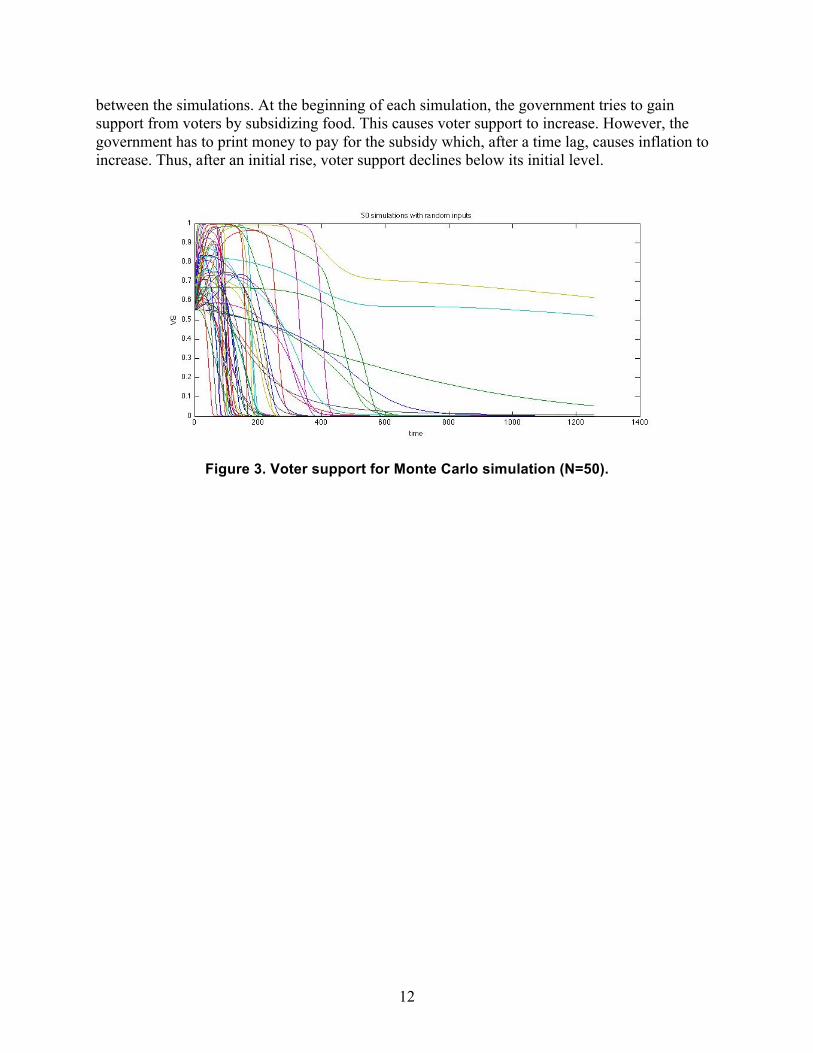
12

between the simulations. At the beginning of each simulation, the government tries to gain

support from voters by subsidizing food. This causes voter support to increase. However, the

government has to print money to pay for the subsidy which, after a time lag, causes inflation to

increase. Thus, after an initial rise, voter support declines below its initial level.

Figure 3. Voter support for Monte Carlo simulation (N=50).

13

14

3. COMPARISON OF METHODS

The goal of this work was to compare different sensitivity analysis techniques to gain insight into

which methods are most appropriate for models of human behavior. Different promising

methods were applied to the food subsidy model, tested, and compared. While different outputs

are certainly of interest in this model, results presented here focus on one output: voter support.

Each analysis method used a sample size of 1000 model runs. Static and dynamic sensitivity

were both considered. For the static analyses, the highest value of voter support over the time

horizon was used as a metric. The dynamic analyses were based on voter support at each point

throughout the time horizon.

The first sensitivity analysis technique considered for the food subsidy model was scatterplots.

Scatterplots necessitate a static output metric, so the highest voter support metric was used as the

output. Each uncertain input was plotted against this metric to look for patterns in the

relationships between inputs and the output metric (figure 4). Scatterplots are especially useful in

finding unusual or unanticipated patterns, such as thresholds and nonlinearities, in the data (Ford

and Flynn 2005; Helton et al. 2006). Relationships to the output metric are apparent for some of

the uncertain inputs to the food subsidy model, particularly EVS and GFSGamma (positive

correlations), and VPBeta (negative correlation). However, none of the inputs are obviously

dominant in determining the highest voter support.

15

Figure 4. Scatterplots of different inputs compared to the highest voter support.

The next method considered was correlation coefficients (Helton et al. 2006). These are used to

measure the strength of the linear relationship between each uncertain input and the output of

interest. Correlation coefficients can be used to rank inputs by importance. Variations of

correlation coefficients are also available. Partial correlation coefficients correct for the linear

effects of other inputs. Rank correlation coefficients consider monotonic, rather than linear

relationships between inputs and outputs. Partial rank correlation coefficients combine these

qualities. Correlation coefficients vary from -1 to 1, with a stronger correlation indicated when

the coefficient is farther from 0. The p-value associated with a correlation coefficient describes

the significance of the correlation, with a small p-value (for instance, p<0.05) indicating high

significance.

16

Two different ways of using correlation coefficients were considered for this analysis. The first

was a static analysis, which looked at how each uncertain input to the food subsidy model

correlates with the output metric highest voter support (table 2). According to the p-values for

each of the different types of correlation coefficients, most of the uncertain inputs have a

significant non-zero correlation with the output metric. Furthermore, the different methods agree

on most of the top (most highly correlated) inputs.

Table 2. Correlation coefficients for highest voter support output metric.

Corr

elat

ion

Coef

fici

ent

CC

p-v

alue

Par

tial

Corr

elat

ion

Coef

fici

ent

PC

C

p-v

alue

Ran

k

Corr

elat

ion

Coef

fici

ent

RC

C

p-v

alue

Par

tial

Ran

k

Corr

elat

ion

Coef

fici

ent

PR

CC

p-v

alue

EVP -0.012 0.716 -0.041 0.196 -0.019 0.541 -0.056 0.080

EVS 0.211 0.000 0.363 0 0.213 0.000 0.375 0

OP -0.086 0.007 -0.046 0.152 -0.078 0.013 -0.073 0.022

PA 0.288 0 0.408 0 0.324 0 0.468 0

FDBeta -0.022 0.496 -0.035 0.275 -0.014 0.649 -0.033 0.296

GFSBeta -0.140 0.000 -0.161 0.000 -0.138 0.000 -0.165 0.000

GFSGamm

a

0.383 0 0.548 0 0.365 0 0.556 0

VPBeta -0.519 0 -0.646 0 -0.528 0 -0.676 0

VPGamma 0.160 0.000 0.220 0.000 0.149 0.000 0.219 0.000

VSBeta 0.103 0.001 0.158 0.000 0.158 0.000 0.248 0.000

VSDelta 0.021 0.509 0.071 0.027 0.101 0.001 0.201 0.000

VSGamma -0.009 0.789 -0.021 0.519 -0.021 0.500 -0.050 0.120

The second correlation coefficient analysis calculated correlation over time (Ford and Flynn

2005) for each uncertain input in relation to voter support. By plotting each type of correlation

coefficient over time, the relative strength of correlations for different inputs during different

times can be seen (figures 5-8). For most inputs, he different types of correlation coefficients

were similar. In the beginning of the simulation, when voter support is increasing, a selection of

inputs is apparently highly correlated with voter support. The collection of highly correlated

inputs seems to change, however, when the behavior of voter support shifts to declining. One

input, VSDelta, is highly negatively correlated toward the end of the simulation only in the rank

and partial rank analyses, indicating a monotonic but not linear relationship between VSDelta

and voter support.

17

Figure 5. Correlation coefficients for voter support over time.

Figure 6. Partial correlation coefficients for voter support over time.

18

Figure 7. Rank correlation coefficients for voter support over time.

Figure 8. Partial rank correlation coefficients for voter support over time.

The next sensitivity analysis implemented was a stepwise regression (Helton et al. 2006) based

on the highest voter support output metric. Stepwise regression creates a linear regression model

by repeatedly adding the most important variable to the model. The process begins by

determining for which input, by itself, would lead to the highest R2 value. R

2 measures the

fraction of output variance that is explained by the model. After the first, most important, input is

found, the next most significant input is searched for and added to the model. This process goes

on until the regression model would not be significantly improved by adding any of the

remaining inputs.

Results for the stepwise regression of the food subsidy model and the output metric highest voter

support are shown in table 3. Nine of the uncertain inputs were useful in the regression model,

with only three considered insignificant. Even with all nine of the useful inputs included, the R2

value is still only 0.6134.

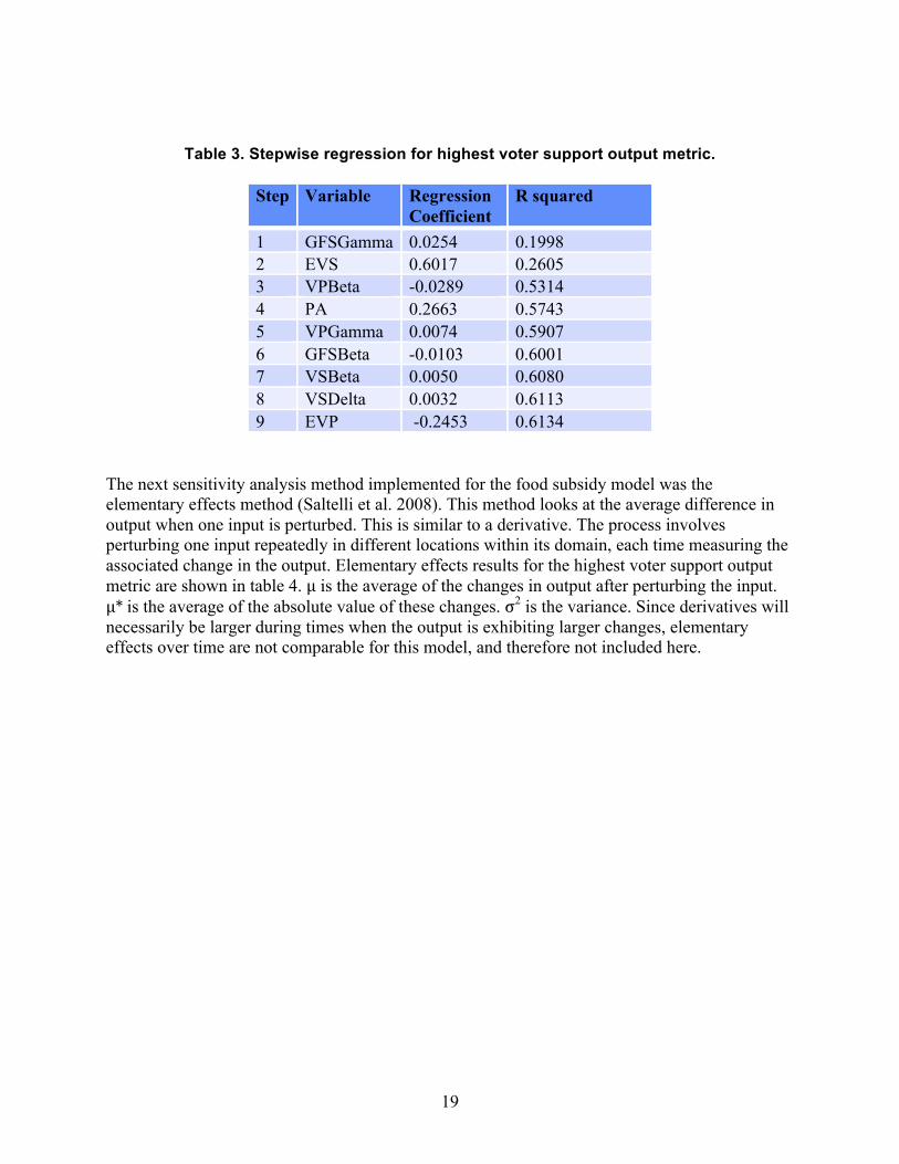
19

Table 3. Stepwise regression for highest voter support output metric.

Step Variable Regression

Coefficient

R squared

1 GFSGamma 0.0254 0.1998

2 EVS 0.6017 0.2605

3 VPBeta -0.0289 0.5314

4 PA 0.2663 0.5743

5 VPGamma 0.0074 0.5907

6 GFSBeta -0.0103 0.6001

7 VSBeta 0.0050 0.6080

8 VSDelta 0.0032 0.6113

9 EVP -0.2453 0.6134

The next sensitivity analysis method implemented for the food subsidy model was the

elementary effects method (Saltelli et al. 2008). This method looks at the average difference in

output when one input is perturbed. This is similar to a derivative. The process involves

perturbing one input repeatedly in different locations within its domain, each time measuring the

associated change in the output. Elementary effects results for the highest voter support output

metric are shown in table 4. ! is the average of the changes in output after perturbing the input.

!"#is the average of the absolute value of these changes. $2 is the variance. Since derivatives will

necessarily be larger during times when the output is exhibiting larger changes, elementary

effects over time are not comparable for this model, and therefore not included here.

20

Table 4. Elementary effects results for highest voter support output metric.

! !"# $2

EVP 0.0091 0.0915 0.0002

EVS -0.0077 0.0855 0.0006

OP -0.0038 0.0809 0.0001

PA -0.0003 0.0987 0.0014

FDBeta 0.0005 0.0916 0.0001

GFSBeta -0.0031 0.0865 0.0002

GFSGamma -0.0003 0.1127 0.0006

VPBeta 0.0071 0.1028 0.0006

VPGamma 0.0073 0.0915 0.0012

VSBeta -0.0030 0.0870 0.0009

VSDelta 0.0080 0.1008 0.0003

VSGamma -0.0054 0.0927 0.0006

The final method considered in this study was sensitivity indices (Saltelli et al. 2008). Two

measures result from this type of analysis. The first is the main effect, Si, which describes the

proportion of the variance in the output of interest that can be attributed to variation in a

particular input. The second measure is the total effects index, STi. This describes the proportion

of the variance of the output of interest that can be attributed not only to one particular input, but

also to all of the interactions that input has with other inputs. These measures can be used to

indicate where reduced uncertainty in inputs would allow the output variance to be reduced.

The sensitivity indices for the static metric, highest voter support, are shown in table 5. Note that

negative indices can result from the approximation method (Archer et al. 1997). Sensitivity

indices over time in relation to voter support are shown in figures 9 and 10. The main effects plot

shows that a few inputs emerge as very important in determining output variance. The total

effects results show that interactions are very important in this model, particularly at the

beginning of the simulation.

21

Table 5. Sensitivity indices for output metric highest voter support.

SI STI

EVP -0.0021 0.9702

EVS -0.0044 0.9778

OP -0.0024 0.9705

PA -0.0017 0.9761

FDBeta -0.0021 0.9703

GFSBeta -0.0036 0.9763

GFSGamma 0.0065 0.9822

VPBeta 0.0087 0.9893

VPGamma -0.0026 0.9722

VSBeta -0.0057 0.9755

VSDelta -0.0013 0.9734

VSGamma -0.0031 0.9715

Figure 9. Main effects over time for voter support output.

22

Figure 10. Total effects over time for voter support output.

23

24

4. CONCLUSIONS

Table 6 shows how each of the above methods of sensitivity analysis ranks the uncertain

variables in the food subsidy model in order of importance. The different types of static

correlation coefficients give similar results, at least for the most important inputs. However, the

dynamic analysis of different types of correlation coefficients (figures 5-8) indicates that one of

the inputs, VSDelta, has a strong monotonic but nonlinear correlation with voter support in the

second half of the time horizon. Stepwise regression gives similar results to the static correlation

coefficient methods. The elementary effects and sensitivity index rankings differ from the others

somewhat.

Table 6. Comparison of importance rankings of uncertain variables.

Corr

elat

ion

Coef

fici

ent

Par

tial

Corr

elat

ion

Coef

fici

ent

Ran

k

Corr

elat

ion

Coef

fici

ent

Par

tial

Ran

k

Corr

elat

ion

Coef

fici

ent

Ste

pw

ise

Reg

ress

ion

Ele

men

tary

Eff

ects

Must

ar

Sen

siti

vit

y

Indic

es S

i

Sen

siti

vit

y

Indic

es S

Ti

EVS 1-4 1-7 1-4 1-8 2 11 11 3

PA 1-4 1-7 1-4 1-8 4 4 4 5

GFSGamma 1-4 1-7 1-4 1-8 1 1 2 2

VPBeta 1-4 1-7 1-4 1-8 3 2 1 1

VPGamma 5 1-7 7 1-8 5 8 8 8

VSBeta 6 1-7 5 1-8 7 9 12 6

GFSBeta 7 1-7 8 1-8 6 10 10 4

EVP 8 11 9 12 9 7 6 12

FDBeta 9 8 11 9 X 6 5 11

OP 10 10 12 11 X 12 7 10

VSGamma 11 12 10 10 X 5 9 9

VSDelta 12 9 6 1-8 8 3 3 7

Table 7 gives an overview of the different methods of sensitivity analysis described here, as well

as some of the main differences and conclusions found in the sensitivity analysis of the food

subsidy model. Scatterplots showed apparent correlations for only a few of the uncertain inputs,

and no unusual relationships were obvious. Correlation coefficients showed that many of the

uncertain inputs were significantly correlated with the static output metric. The different

methods of calculation did not result in very different coefficients for the static analysis, but

understanding of one uncertain input benefited from calculation of rank correlation coefficients

in the dynamic analysis. The stepwise regression analysis gave similar results to the correlation

coefficient analysis, and thus was probably an unnecessary calculation for the food subsidy

25

model. The elementary effects analysis showed that many of the inputs were similar in

importance. The sensitivity indices showed that interactions between inputs were significant,

especially during the beginning of the simulation.

Table 7. Comparison and implications for different methods of sensitivity analysis.

Method What is measured Comparison and implications

Scatterplots

Subjective relationship

between inputs and outputs

•Good first method for identifying

patterns

•No very obvious patterns

Correlation Coefficients

Strength of linear (or

monotonic) relationship

•Useful in ranking inputs

•Static results similar for different

types of CC, dynamic results

differed for one input

Stepwise Regression

Coefficients for linear model

that best predicts output

•Most inputs were significant

•Results similar to correlation

coefficients

Elementary Effects

Average derivative when one

input is perturbed over

different points in its domain

•Little variation in µ* between

inputs

Sensitivity Indices Proportion of output variance

attributed to input variance

•Interactions were significant

•Especially important at the

beginning of the simulation

No one, or few, inputs dominated the results of the food subsidy model. Interactions between

inputs, however, did play a large role, particularly at the beginning of the simulation. It is

important to note that the results above apply to only the food subsidy model. More

investigation, into different models, different output metrics, and different techniques of

sensitivity analysis, is needed to determine if these results apply more generally to models of

human behavior.

26

27

5. REFERENCES

1. Archer, G.E.B., Saltelli, A., and I.M. Sobol. 1997. Sensitivity measures, ANOVE-like

techniques and the use of bootstrap. Journal of Statistical Computation and Simulation.

58: 99-120.

2. Ben-Akiva, Moshe, and Steven R. Lerman. 1985. Discrete Choice Analysis: Theory

and Application to Travel Demand. MIT Press: Cambridge, MA.

3. Ford, Andrew, and Hilary Flynn. 2005. Statistical screening of system dynamics models.

System Dynamics Review. 21 (4): 273-303.

4. Hekimoglu, Mustafa. 2010. Sensitivity analysis of oscillatory system dynamics models.

Proceedings of the 28th

International Conference of the System Dynamics Society, July 25

– July 29, 2010.

5. Helton, J.C., Johnson, J.D., Sallaberry, C.J., and C.B. Storlie. 2006. Survey of sampling-

based methods for uncertainty and sensitivity analysis. SAND2006-2901.

6. National Research Council (NRC). 2008. Behavioral modeling and simulation: From

individuals to societies. The National Academies Press, Washington, DC.

7. Saltelli, A., Ratto, M., Andres, T., Campolongo, F., Cariboni, J., Gatelli, D., Saisana, M.,

and S. Tarantola. 2008. Global Sensitivity Analysis: The Primer. John Wiley & Sons,

Ltd: Chichester, West Sussex, England.

8. Train, Kenneth. 1986. Qualitative Choice Analysis. MIT Press: Cambridge,

Massachusetts.

28