Sensitivity Analysis in Observational Research: Introducing the E-value

Tyler J. VanderWeeleHarvard T.H. Chan School of Public Health

Departments of Epidemiology and Biostatistics

1

Plan of Presentation

(1) Introduction to Sensitivity Analysis

(2) Cornfield Conditions

(3) E-values for Sensitivity Analysis

(4) Empirical Examples

(5) Other Scales

- Hazard Ratios, Odds Ratios, Continuous Outcomes

(6) Other Sensitivity Analysis Results

(7) Concluding Remarks

2

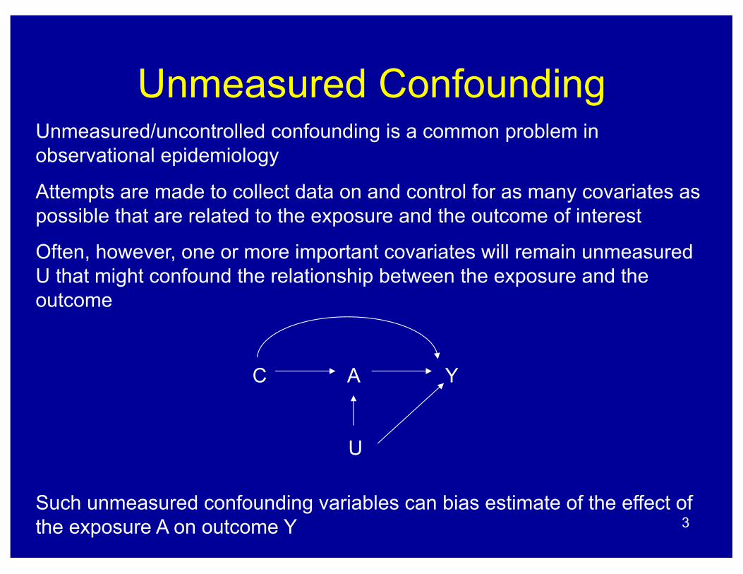
Unmeasured ConfoundingUnmeasured/uncontrolled confounding is a common problem in observational epidemiology

Attempts are made to collect data on and control for as many covariates as possible that are related to the exposure and the outcome of interest

Often, however, one or more important covariates will remain unmeasured U that might confound the relationship between the exposure and the outcome

Such unmeasured confounding variables can bias estimate of the effect of the exposure A on outcome Y

C A Y

U

3

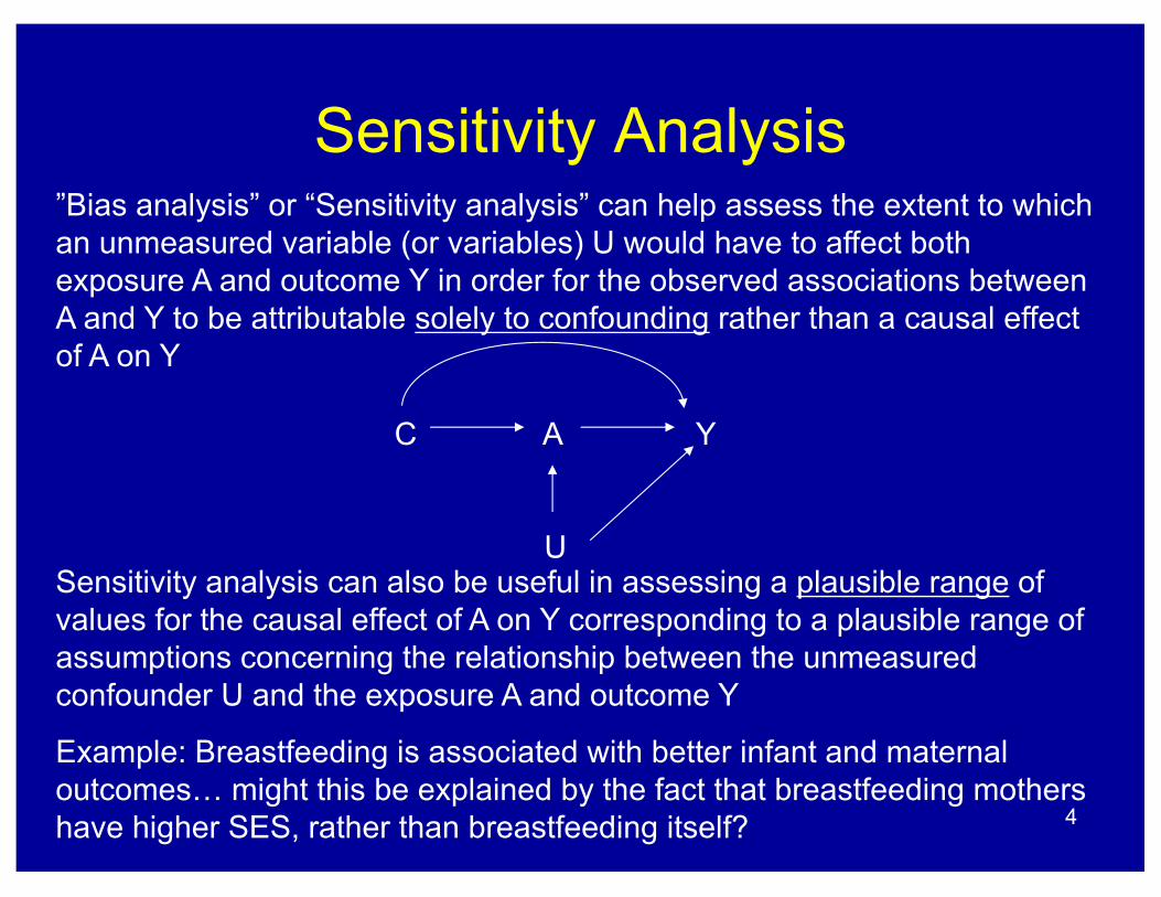
Sensitivity Analysis”Bias analysis” or “Sensitivity analysis” can help assess the extent to which an unmeasured variable (or variables) U would have to affect both exposure A and outcome Y in order for the observed associations between A and Y to be attributable solely to confounding rather than a causal effect of A on Y

Sensitivity analysis can also be useful in assessing a plausible range of values for the causal effect of A on Y corresponding to a plausible range of assumptions concerning the relationship between the unmeasured confounder U and the exposure A and outcome Y

Example: Breastfeeding is associated with better infant and maternal outcomes… might this be explained by the fact that breastfeeding mothers have higher SES, rather than breastfeeding itself?

C A Y

U

4

Sensitivity Analysis

The term “sensitivity analysis” is used outside the context of unmeasured confounding bias to address other types of bias such as selection bias and measurement error

In other fields “sensitivity analysis” is also referred to as “bias analysis” (e.g. Rothman et al., 2008; Lash et al., 2009)

An early application of this approach was the work of Cornfield et al. (1959) who showed that the association between smoking and lung-cancer association was unlikely to be entirely due to unmeasured confounding by an unknown genetic factor

5

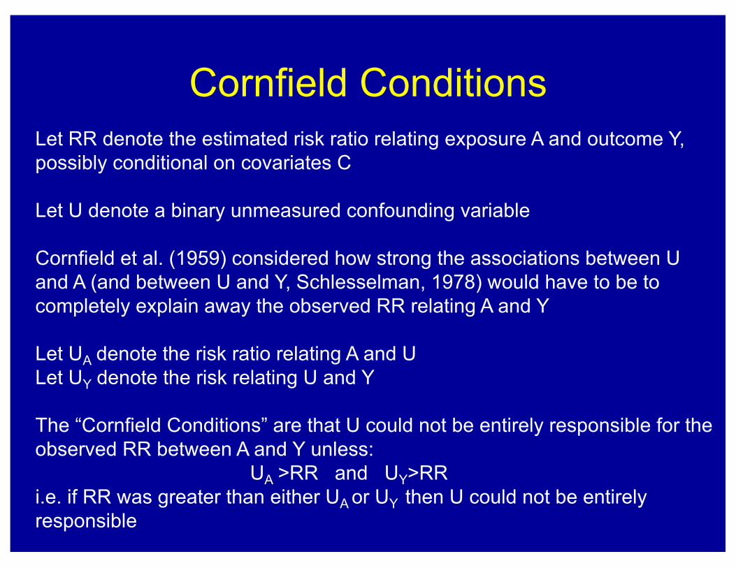
Cornfield ConditionsLet RR denote the estimated risk ratio relating exposure A and outcome Y, possibly conditional on covariates C

Let U denote a binary unmeasured confounding variable

Cornfield et al. (1959) considered how strong the associations between U and A (and between U and Y, Schlesselman, 1978) would have to be to completely explain away the observed RR relating A and Y

Let UA denote the risk ratio relating A and ULet UY denote the risk relating U and Y

The “Cornfield Conditions” are that U could not be entirely responsible for the observed RR between A and Y unless:

UA >RR and UY>RR i.e. if RR was greater than either UA or UY then U could not be entirely responsible

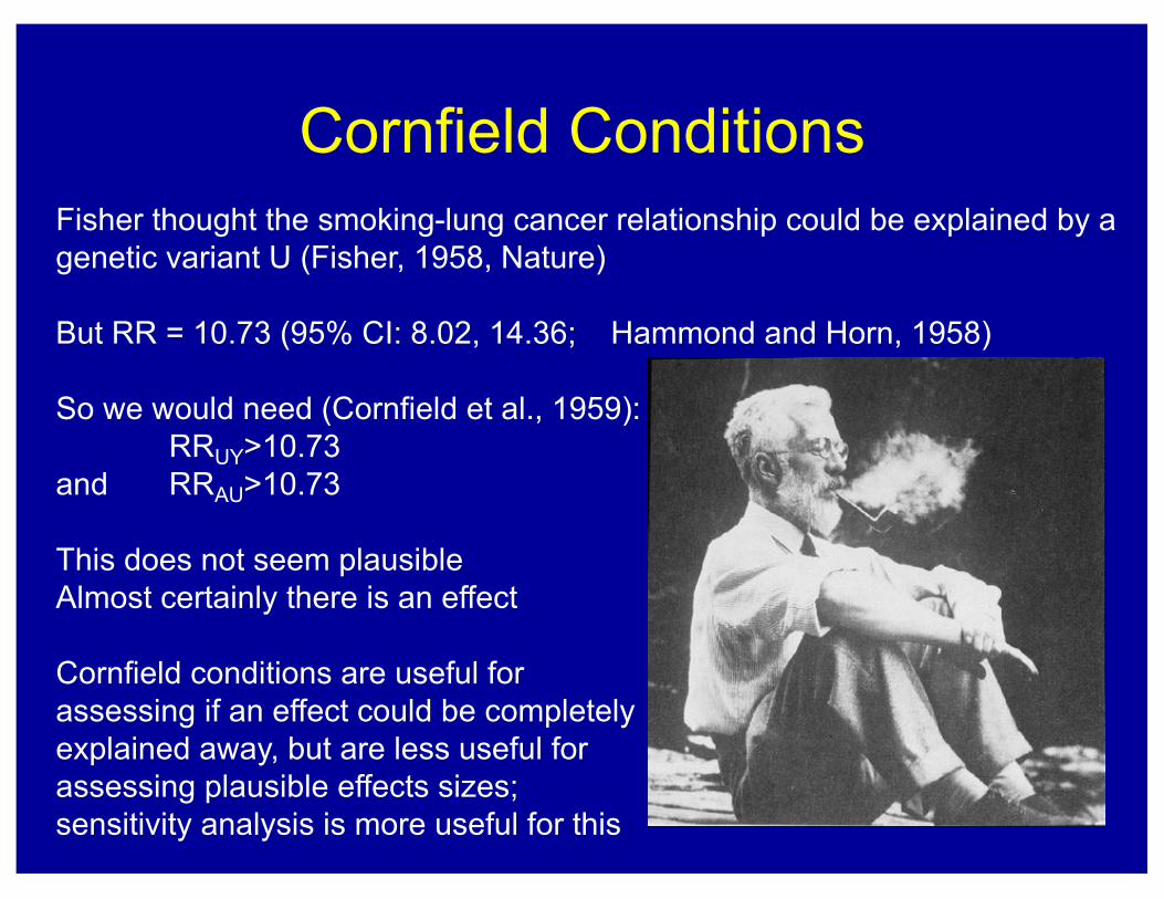
Cornfield ConditionsFisher thought the smoking-lung cancer relationship could be explained by a genetic variant U (Fisher, 1958, Nature)

But RR = 10.73 (95% CI: 8.02, 14.36; Hammond and Horn, 1958)

So we would need (Cornfield et al., 1959):RRUY>10.73

and RRAU>10.73

This does not seem plausibleAlmost certainly there is an effect

Cornfield conditions are useful for assessing if an effect could be completelyexplained away, but are less useful for assessing plausible effects sizes;sensitivity analysis is more useful for this

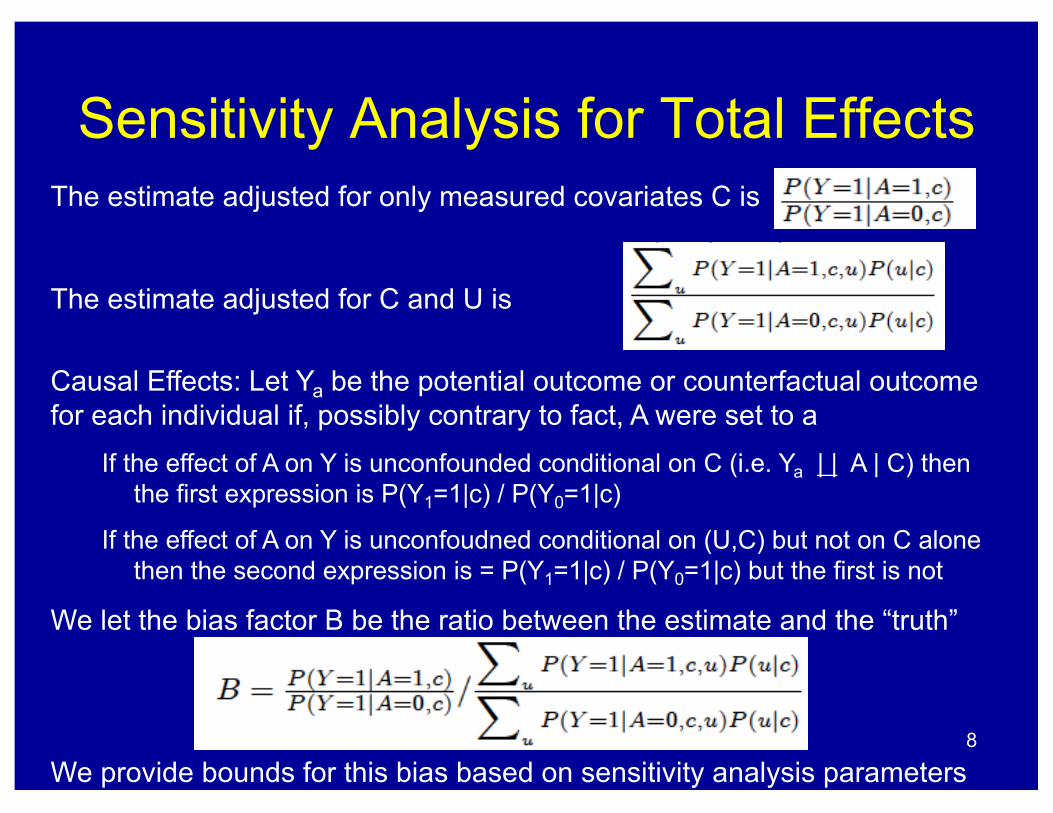
Sensitivity Analysis for Total EffectsThe estimate adjusted for only measured covariates C is

The estimate adjusted for C and U is

Causal Effects: Let Ya be the potential outcome or counterfactual outcome for each individual if, possibly contrary to fact, A were set to a

If the effect of A on Y is unconfounded conditional on C (i.e. Ya | | A | C) then the first expression is P(Y1=1|c) / P(Y0=1|c)

If the effect of A on Y is unconfoudned conditional on (U,C) but not on C alone then the second expression is = P(Y1=1|c) / P(Y0=1|c) but the first is not

We let the bias factor B be the ratio between the estimate and the “truth”

We provide bounds for this bias based on sensitivity analysis parameters8

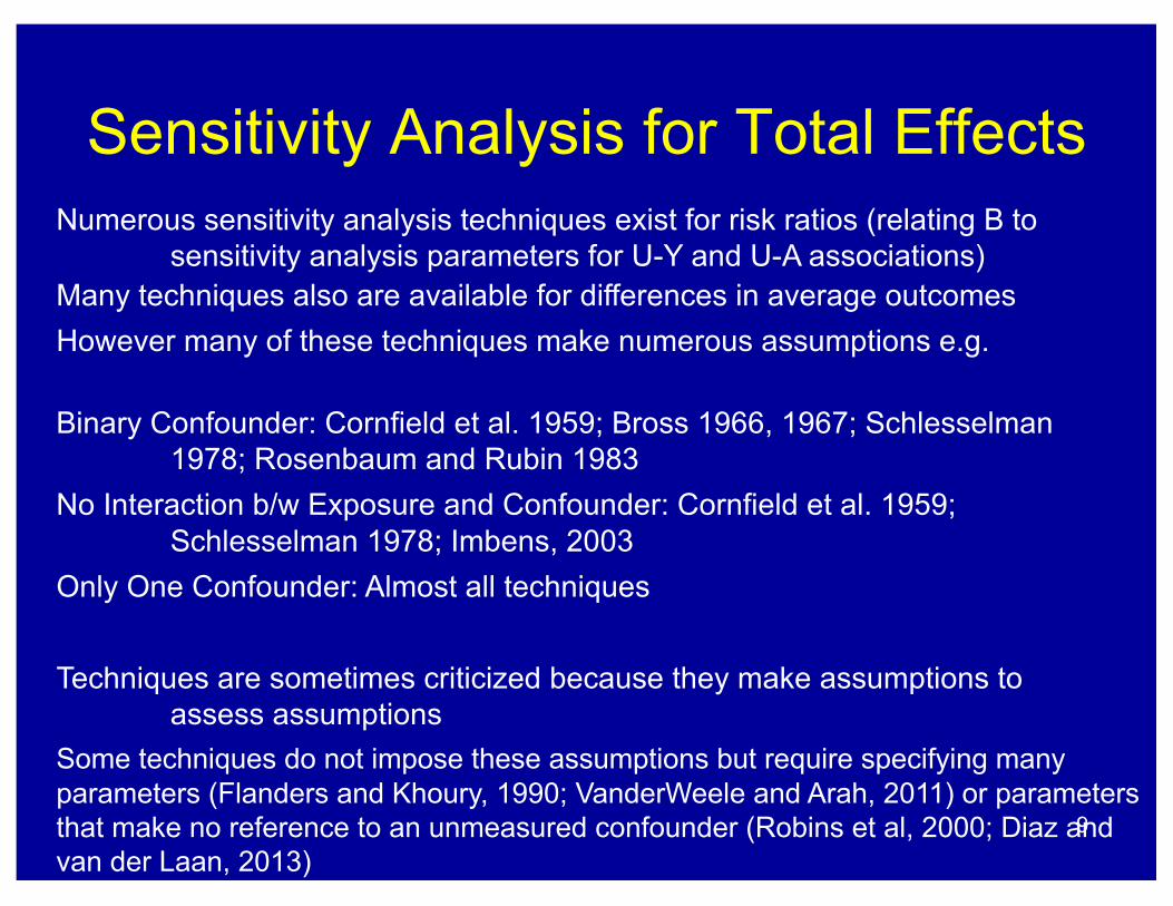
Sensitivity Analysis for Total EffectsNumerous sensitivity analysis techniques exist for risk ratios (relating B to

sensitivity analysis parameters for U-Y and U-A associations)Many techniques also are available for differences in average outcomesHowever many of these techniques make numerous assumptions e.g.

Binary Confounder: Cornfield et al. 1959; Bross 1966, 1967; Schlesselman 1978; Rosenbaum and Rubin 1983

No Interaction b/w Exposure and Confounder: Cornfield et al. 1959; Schlesselman 1978; Imbens, 2003

Only One Confounder: Almost all techniques

Techniques are sometimes criticized because they make assumptions to assess assumptions

Some techniques do not impose these assumptions but require specifying many parameters (Flanders and Khoury, 1990; VanderWeele and Arah, 2011) or parameters that make no reference to an unmeasured confounder (Robins et al, 2000; Diaz and van der Laan, 2013)

9

Sensitivity Analysis w/o AssumptionsHere we give an approach that in some sense makes “no assumptions” (Ding and VanderWeele, 2016)

Assume we have one or more unmeasured confounders UWe define the following parameters

These are essentially the maximum effect of U on Y across exposure groups and the maximum risk ratio relating A and any category of UIf U is binary these are just ordinary risk ratios, but apply more generally

Note that the parameters condition on the measured covariate CThey capture the confounding after having already controlled for C

10

Sensitivity Analysis w/o AssumptionsLet RRUY be the maximum risk ratio relating any two categories of

U to Y conditional on covariates C and across exposure ALet RRAU be the maximum risk ratio relating A to any category of U

The largest factor by which such a U could reduce an observed risk ratio estimate is given by (Ding and VanderWeele (2016, Epidemiology):

B = RRUY*RRAU

(RRUY+RRAU - 1)

We can divide the estimate and CI by B to obtain a “corrected” estimate and CI (i.e. the maximum a confounder could shift the estimate)The result holds without making any assumptions about the structure of UThe bound is “sharp” in the sense that some U can always achieve themIf the association is protective we multiply rather than divide

11

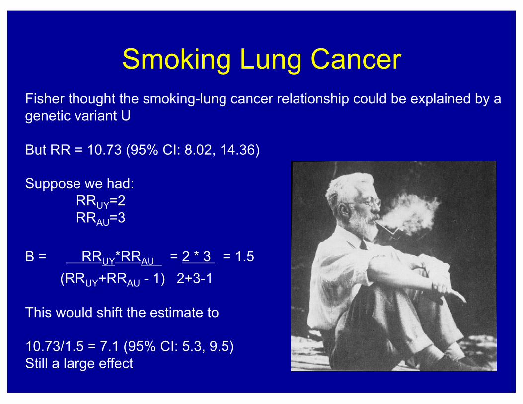
Smoking Lung CancerFisher thought the smoking-lung cancer relationship could be explained by a genetic variant U

But RR = 10.73 (95% CI: 8.02, 14.36)

Suppose we had:RRUY=2RRAU=3

B = RRUY*RRAU = 2 * 3 = 1.5(RRUY+RRAU - 1) 2+3-1

This would shift the estimate to

10.73/1.5 = 7.1 (95% CI: 5.3, 9.5)Still a large effect

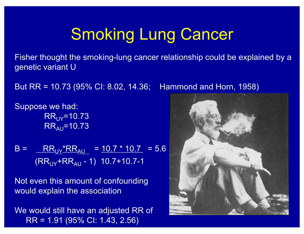
Smoking Lung CancerFisher thought the smoking-lung cancer relationship could be explained by a genetic variant U

But RR = 10.73 (95% CI: 8.02, 14.36; Hammond and Horn, 1958)

Suppose we had:RRUY=10.73RRAU=10.73

B = RRUY*RRAU = 10.7 * 10.7 = 5.6(RRUY+RRAU - 1) 10.7+10.7-1

Not even this amount of confoundingwould explain the association

We would still have an adjusted RR ofRR = 1.91 (95% CI: 1.43, 2.56)

Sensitivity Analysis w/o Assumptions

The Cornfield conditions are generally conservative

The largest factor by which such a U could reduce an observed risk ratio estimate is given by (take inverses for protective exposures):

B = RRUY*RRAU

(RRUY+RRAU - 1)

If we let RRUY go to infinity we get B = RRAU

If we let RRUA go to infinity we get B = RRUY

i.e. we recover the Cornfield Conditions (but without assuming a binary confounder); the Cornfield conditions essentially assume the other parameter is infinite; it is conservative in the other parameter 14

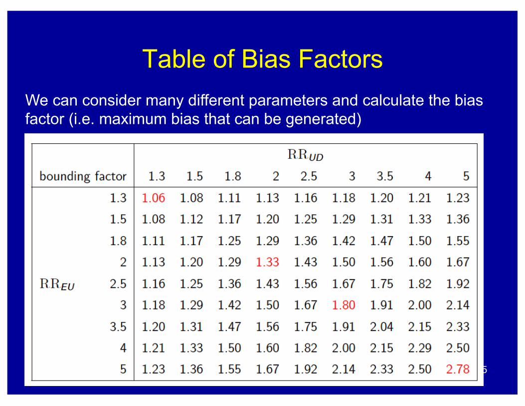
We can consider many different parameters and calculate the bias factor (i.e. maximum bias that can be generated)

Table of Bias Factors

15

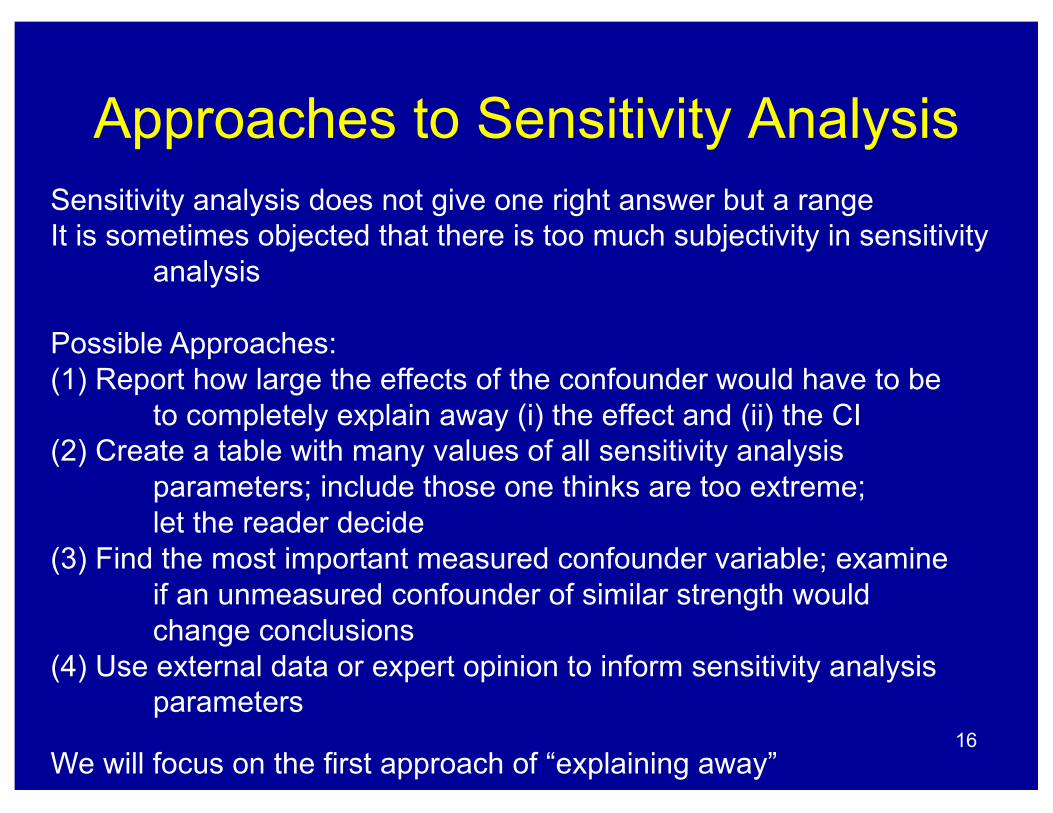
Sensitivity analysis does not give one right answer but a rangeIt is sometimes objected that there is too much subjectivity in sensitivity

analysis

Possible Approaches:(1) Report how large the effects of the confounder would have to be

to completely explain away (i) the effect and (ii) the CI(2) Create a table with many values of all sensitivity analysis

parameters; include those one thinks are too extreme;let the reader decide

(3) Find the most important measured confounder variable; examine if an unmeasured confounder of similar strength wouldchange conclusions

(4) Use external data or expert opinion to inform sensitivity analysis parameters

We will focus on the first approach of “explaining away”

Approaches to Sensitivity Analysis

16

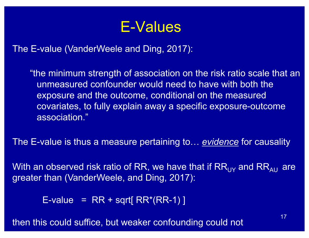
E-ValuesThe E-value (VanderWeele and Ding, 2017):

“the minimum strength of association on the risk ratio scale that an unmeasured confounder would need to have with both the exposure and the outcome, conditional on the measured covariates, to fully explain away a specific exposure-outcome association.”

The E-value is thus a measure pertaining to… evidence for causality

With an observed risk ratio of RR, we have that if RRUY and RRAU are greater than (VanderWeele, and Ding, 2017):

E-value = RR + sqrt[ RR*(RR-1) ]

then this could suffice, but weaker confounding could not17

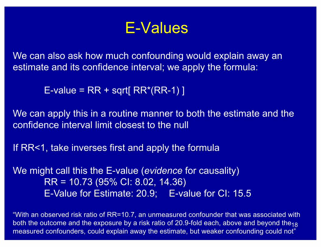
E-ValuesWe can also ask how much confounding would explain away an estimate and its confidence interval; we apply the formula:

E-value = RR + sqrt[ RR*(RR-1) ]

We can apply this in a routine manner to both the estimate and the confidence interval limit closest to the null

If RR<1, take inverses first and apply the formula

We might call this the E-value (evidence for causality)RR = 10.73 (95% CI: 8.02, 14.36)E-Value for Estimate: 20.9; E-value for CI: 15.5

“With an observed risk ratio of RR=10.7, an unmeasured confounder that was associated with both the outcome and the exposure by a risk ratio of 20.9-fold each, above and beyond the measured confounders, could explain away the estimate, but weaker confounding could not”

18

Sensitivity Analysis w/o Assumptions

Smoking and Lung Cancer (Hammond and Horn, 1958):

RR = 10.73 (95% CI: 8.02, 14.36)

19

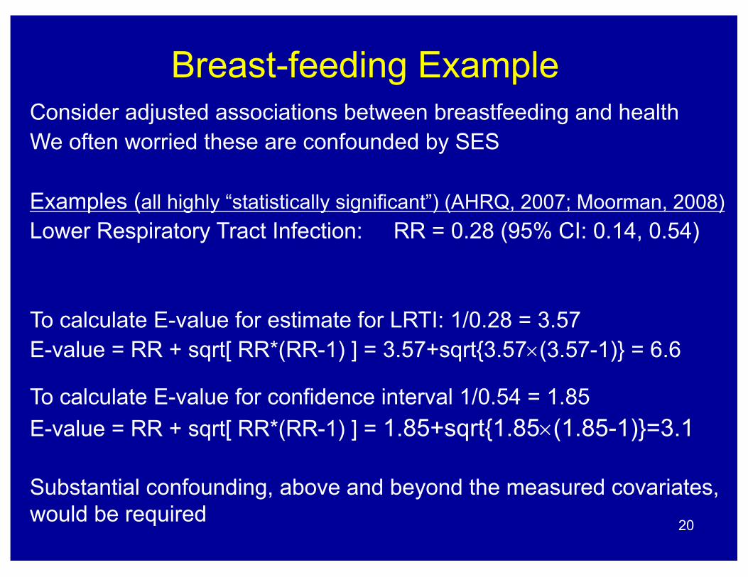
Breast-feeding ExampleConsider adjusted associations between breastfeeding and healthWe often worried these are confounded by SES

Examples (all highly “statistically significant”) (AHRQ, 2007; Moorman, 2008)Lower Respiratory Tract Infection: RR = 0.28 (95% CI: 0.14, 0.54)

To calculate E-value for estimate for LRTI: 1/0.28 = 3.57E-value = RR + sqrt[ RR*(RR-1) ] = 3.57+sqrt{3.57´(3.57-1)} = 6.6

To calculate E-value for confidence interval 1/0.54 = 1.85E-value = RR + sqrt[ RR*(RR-1) ] = 1.85+sqrt{1.85´(1.85-1)}=3.1

Substantial confounding, above and beyond the measured covariates, would be required 20

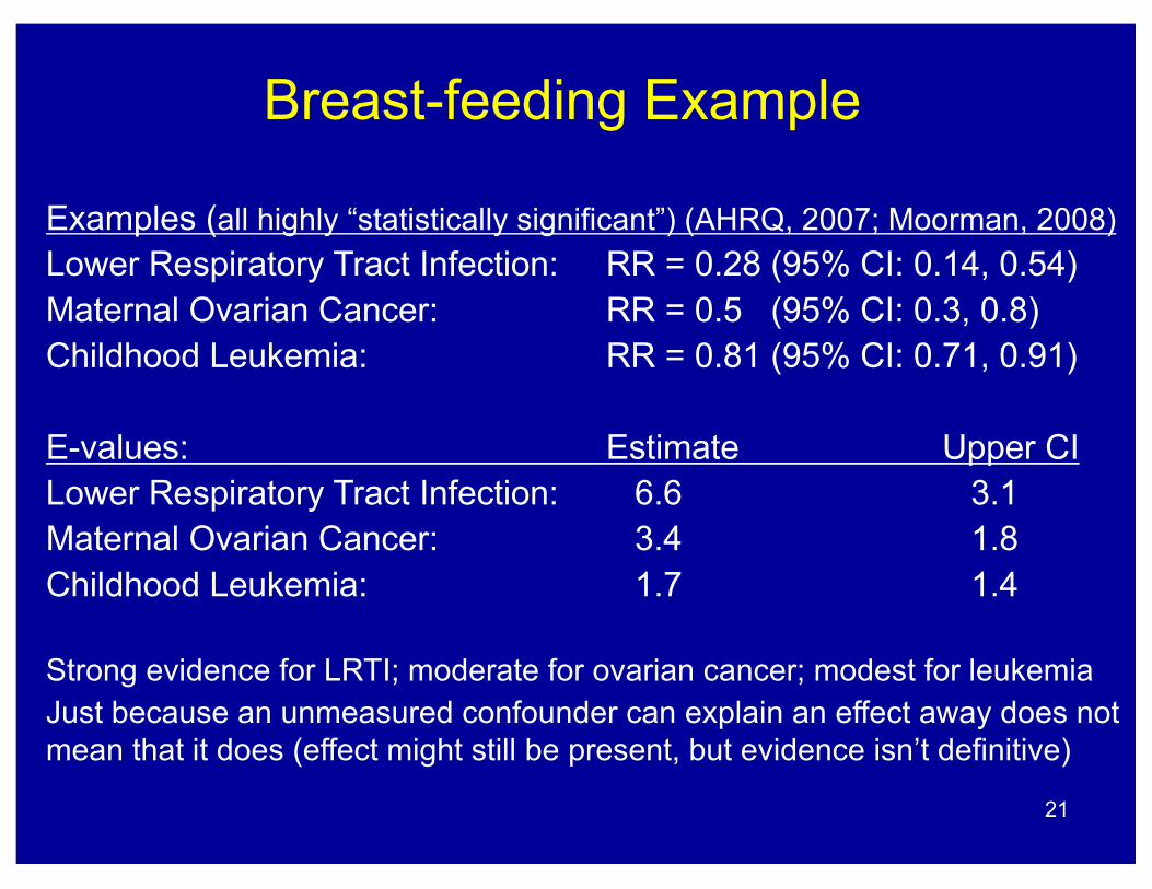
Breast-feeding Example

Examples (all highly “statistically significant”) (AHRQ, 2007; Moorman, 2008)Lower Respiratory Tract Infection: RR = 0.28 (95% CI: 0.14, 0.54)Maternal Ovarian Cancer: RR = 0.5 (95% CI: 0.3, 0.8)Childhood Leukemia: RR = 0.81 (95% CI: 0.71, 0.91)

E-values: Estimate Upper CILower Respiratory Tract Infection: 6.6 3.1Maternal Ovarian Cancer: 3.4 1.8Childhood Leukemia: 1.7 1.4

Strong evidence for LRTI; moderate for ovarian cancer; modest for leukemiaJust because an unmeasured confounder can explain an effect away does not mean that it does (effect might still be present, but evidence isn’t definitive)

21

E-ValuesE-value Formula: E-value = RR + sqrt[ RR*(RR-1) ]

The E-value could always be reported for the estimate and CIThis would allow for better assessment of causality

P-value gives evidence for associationE-value gives evidence that the association is causal

The two can diverge: E-values: Estimate Upper CIMaternal Ovarian Cancer: 3.4 1.8Childhood Leukemia: 1.7 1.4

P-value is more extreme for leukemia (p<.001) than ovarian cancer (P=.006)E-value is more extreme for ovarian cancer than leukemia 22

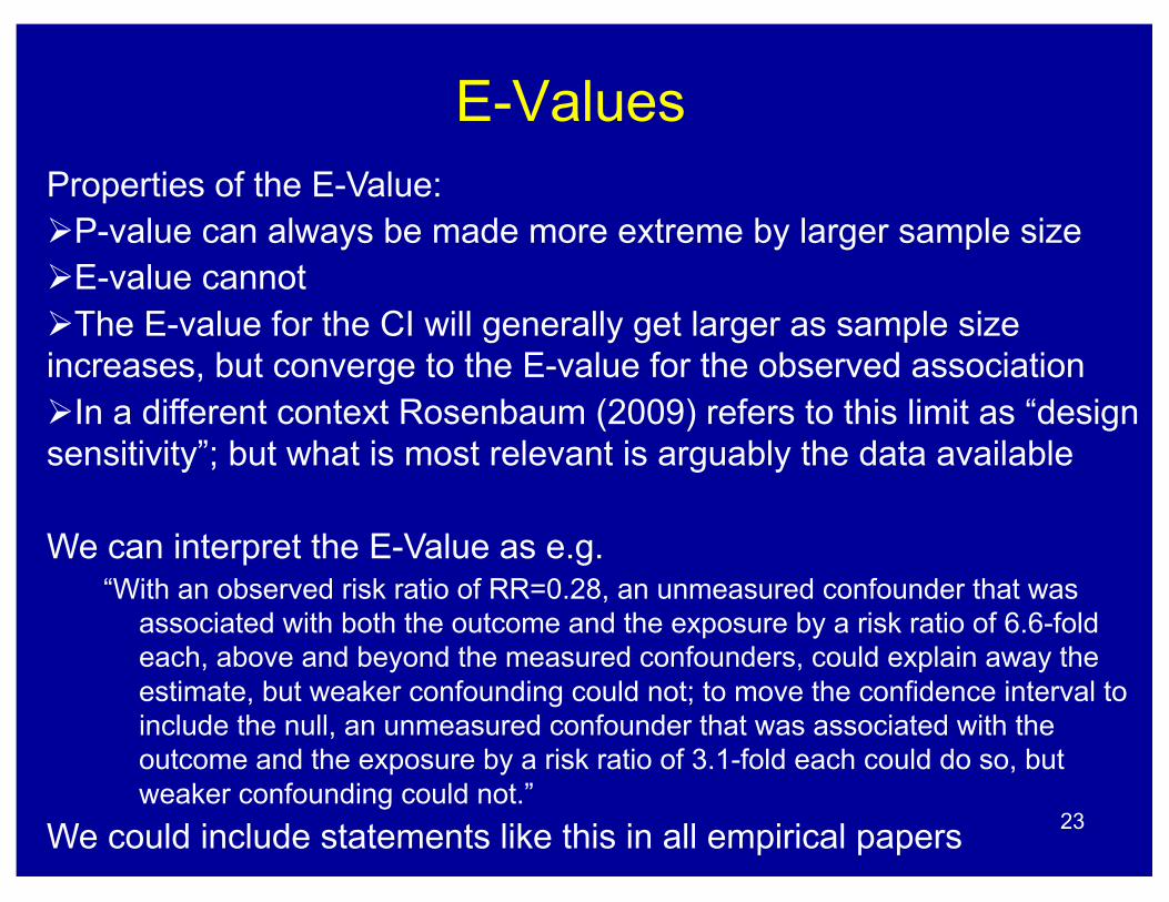
E-ValuesProperties of the E-Value:ØP-value can always be made more extreme by larger sample sizeØE-value cannot ØThe E-value for the CI will generally get larger as sample size increases, but converge to the E-value for the observed associationØIn a different context Rosenbaum (2009) refers to this limit as “design sensitivity”; but what is most relevant is arguably the data available

We can interpret the E-Value as e.g.“With an observed risk ratio of RR=0.28, an unmeasured confounder that was

associated with both the outcome and the exposure by a risk ratio of 6.6-fold each, above and beyond the measured confounders, could explain away the estimate, but weaker confounding could not; to move the confidence interval to include the null, an unmeasured confounder that was associated with the outcome and the exposure by a risk ratio of 3.1-fold each could do so, but weaker confounding could not.”

We could include statements like this in all empirical papers 23

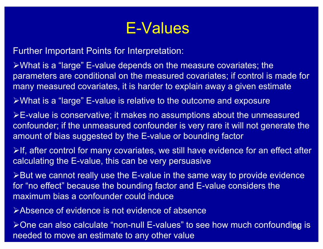
E-ValuesFurther Important Points for Interpretation:ØWhat is a “large” E-value depends on the measure covariates; the parameters are conditional on the measured covariates; if control is made for many measured covariates, it is harder to explain away a given estimateØWhat is a “large” E-value is relative to the outcome and exposureØE-value is conservative; it makes no assumptions about the unmeasured confounder; if the unmeasured confounder is very rare it will not generate the amount of bias suggested by the E-value or bounding factorØIf, after control for many covariates, we still have evidence for an effect after calculating the E-value, this can be very persuasiveØBut we cannot really use the E-value in the same way to provide evidence for “no effect” because the bounding factor and E-value considers the maximum bias a confounder could induceØAbsence of evidence is not evidence of absenceØOne can also calculate “non-null E-values” to see how much confounding is needed to move an estimate to any other value

24

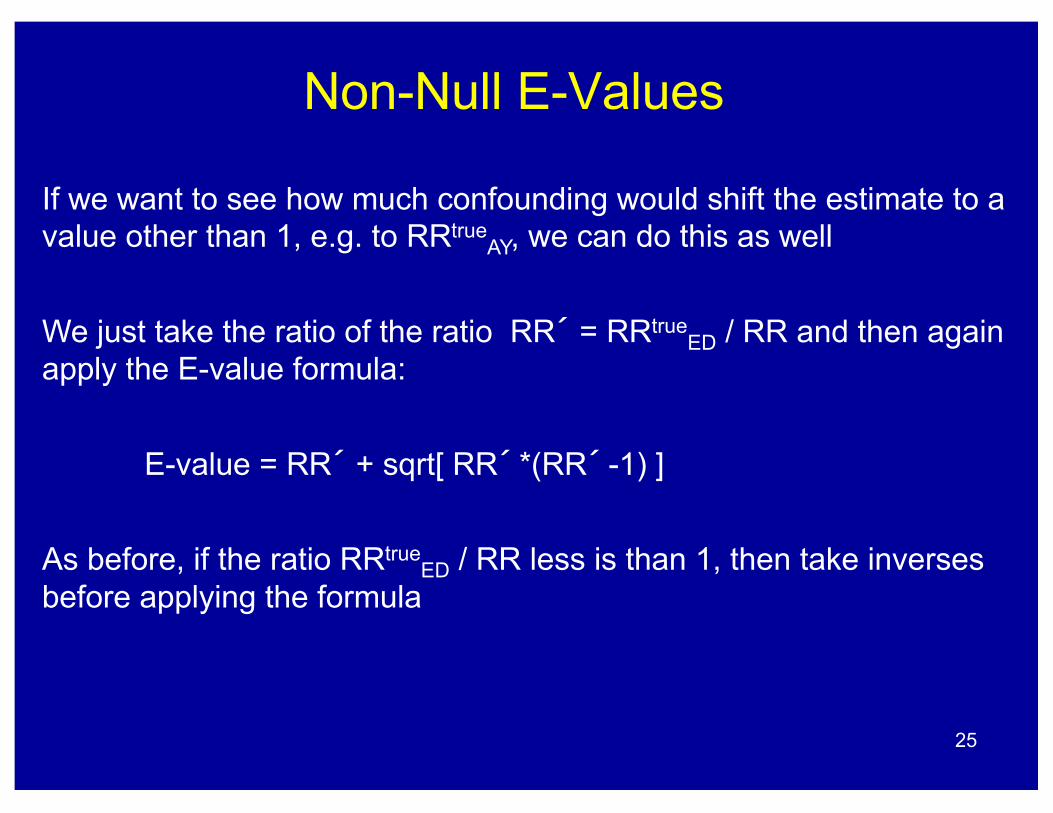
Non-Null E-Values

If we want to see how much confounding would shift the estimate to a value other than 1, e.g. to RRtrue

AY, we can do this as well

We just take the ratio of the ratio RR´ = RRtrueED / RR and then again

apply the E-value formula:

E-value = RR´ + sqrt[ RR´ *(RR´ -1) ]

As before, if the ratio RRtrueED / RR less is than 1, then take inverses

before applying the formula

25

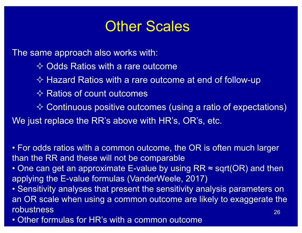
Other ScalesThe same approach also works with:

² Odds Ratios with a rare outcome ² Hazard Ratios with a rare outcome at end of follow-up² Ratios of count outcomes² Continuous positive outcomes (using a ratio of expectations)

We just replace the RR’s above with HR’s, OR’s, etc.

• For odds ratios with a common outcome, the OR is often much larger than the RR and these will not be comparable• One can get an approximate E-value by using RR ≈ sqrt(OR) and then applying the E-value formulas (VanderWeele, 2017)• Sensitivity analyses that present the sensitivity analysis parameters on an OR scale when using a common outcome are likely to exaggerate the robustness• Other formulas for HR’s with a common outcome

26

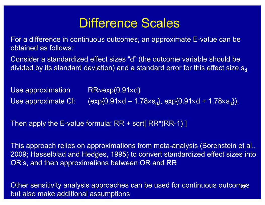
Difference ScalesFor a difference in continuous outcomes, an approximate E-value can be obtained as follows:Consider a standardized effect sizes “d” (the outcome variable should be divided by its standard deviation) and a standard error for this effect size sd

Use approximation RR»exp(0.91´d) Use approximate CI: (exp{0.91´d – 1.78´sd}, exp{0.91´d + 1.78´sd}).

Then apply the E-value formula: RR + sqrt[ RR*(RR-1) ]

This approach relies on approximations from meta-analysis (Borenstein et al., 2009; Hasselblad and Hedges, 1995) to convert standardized effect sizes into OR’s, and then approximations between OR and RR

Other sensitivity analysis approaches can be used for continuous outcomes but also make additional assumptions

27

Advantages of E-Values

Advantages of E-values:(1) Easy to compute

Ø By hand, or with an online calculator, or R package: https://evalue.hmdc.harvard.edu/app/

(2) Easy to report and interpret(3) Standardized metric across different scales(4) Can be calculated “without assumptions”(5) Removal of subjectivity in sensitivity analysis(6) Moving away from OR parameters avoids exaggeration

When to avoid?Possibly when the unmeasured confounder is known and rare

since the E-value approach will be too conservative 28

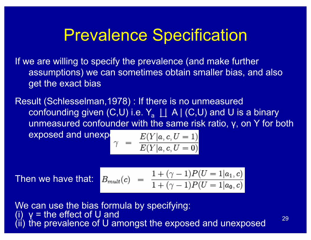
Prevalence SpecificationIf we are willing to specify the prevalence (and make further

assumptions) we can sometimes obtain smaller bias, and also get the exact bias

Result (Schlesselman,1978) : If there is no unmeasured confounding given (C,U) i.e. Ya | | A | (C,U) and U is a binary unmeasured confounder with the same risk ratio, γ, on Y for both exposed and unexposed so that

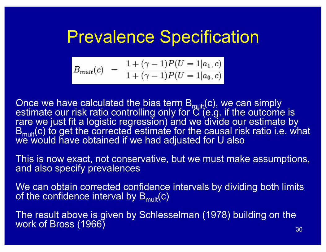
Then we have that:

We can use the bias formula by specifying: (i) γ = the effect of U and (ii) the prevalence of U amongst the exposed and unexposed 29

Prevalence Specification

Once we have calculated the bias term Bmult(c), we can simply estimate our risk ratio controlling only for C (e.g. if the outcome is rare we just fit a logistic regression) and we divide our estimate by Bmult(c) to get the corrected estimate for the causal risk ratio i.e. what we would have obtained if we had adjusted for U also

This is now exact, not conservative, but we must make assumptions, and also specify prevalences

We can obtain corrected confidence intervals by dividing both limits of the confidence interval by Bmult(c)

The result above is given by Schlesselman (1978) building on the work of Bross (1966)

30

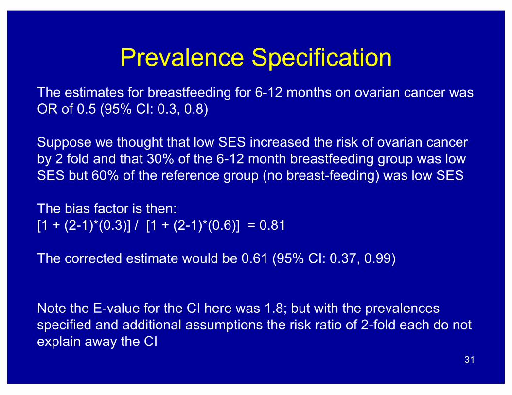
Prevalence SpecificationThe estimates for breastfeeding for 6-12 months on ovarian cancer was OR of 0.5 (95% CI: 0.3, 0.8)

Suppose we thought that low SES increased the risk of ovarian cancer by 2 fold and that 30% of the 6-12 month breastfeeding group was low SES but 60% of the reference group (no breast-feeding) was low SES

The bias factor is then:[1 + (2-1)*(0.3)] / [1 + (2-1)*(0.6)] = 0.81

The corrected estimate would be 0.61 (95% CI: 0.37, 0.99)

Note the E-value for the CI here was 1.8; but with the prevalences specified and additional assumptions the risk ratio of 2-fold each do not explain away the CI

31

Prevalence Specification

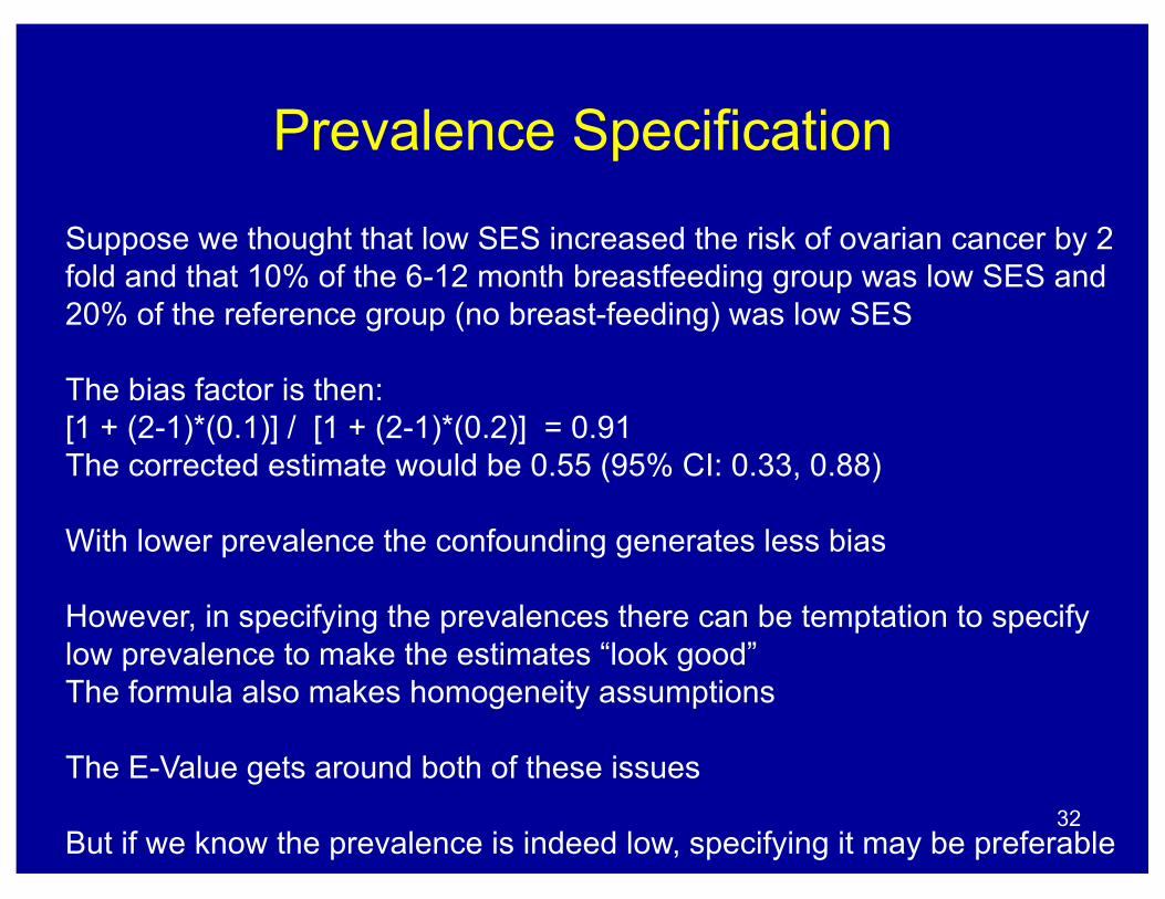
Suppose we thought that low SES increased the risk of ovarian cancer by 2 fold and that 10% of the 6-12 month breastfeeding group was low SES and 20% of the reference group (no breast-feeding) was low SES

The bias factor is then:[1 + (2-1)*(0.1)] / [1 + (2-1)*(0.2)] = 0.91The corrected estimate would be 0.55 (95% CI: 0.33, 0.88)

With lower prevalence the confounding generates less bias

However, in specifying the prevalences there can be temptation to specify low prevalence to make the estimates “look good”The formula also makes homogeneity assumptions

The E-Value gets around both of these issues

But if we know the prevalence is indeed low, specifying it may be preferable32

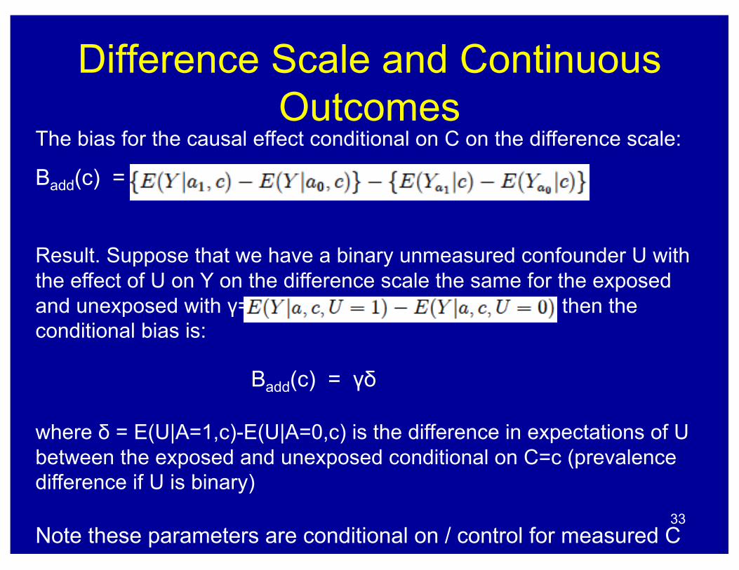
The bias for the causal effect conditional on C on the difference scale:

Badd(c) =

Result. Suppose that we have a binary unmeasured confounder U with the effect of U on Y on the difference scale the same for the exposed and unexposed with γ= then the conditional bias is:

Badd(c) = γδ

where δ = E(U|A=1,c)-E(U|A=0,c) is the difference in expectations of U between the exposed and unexposed conditional on C=c (prevalence difference if U is binary)

Note these parameters are conditional on / control for measured C

Difference Scale and Continuous Outcomes

33

Difference Scale and Continuous Outcomes

Once we have calculated the bias term Badd(c) we can simply estimate our causal effect conditional on C and then subtract the bias term to get the corrected estimate

To get corrected confidence intervals on can simply subtract γδ from both limits of the estimated confidence intervals for either conditional effects or for average causal effects if Badd(c) is constant over c

The result was given in a regression context by Cochran (1935) and re-derived numerous times subsequently, though with increasingly weaker assumptions (Lin et al., 1998; VanderWeele and Arah, 2011)

It can be applied regardless of the estimation method and requires only that the effect of U on Y is the same in both exposure strata (no U*A interaction on the difference scale)But this approach still does make this homogeneity assumption

34

Covariate ConditioningØ All of the results (and all sensitivity analysis parameters) are conditional on

measured covariatesØ Unmeasured confounding, to alter the estimate, must affect the exposure and

outcome through pathways independent of the measured covariates

Ø Often, with extensive confounding control, an additional covariate (which may make a big difference when adjusting compared to the crude estimate) doesn’t matter much under control for other covariate

Ø E.g. “Income” may not matter as much if we have also controlled for education, wealth, home ownership, and occupation

Ø It can be instructive examining this with one’s data

Ø Sensitivity methods (e.g. Altonji et al., 2005) that assume unobserved confounding is comparable in magnitude to observed confounding are problematic b/c it looks like confounding gets worse with additional control

Ø Somewhat more sensible is to compare what proportion of the effect of measured confounding the unobserved confounding would have to have to explain away the effect (Altonji et al., 2005)

Ø Interpretation here as well is also with respect to the measured covariates35

Conclusions

1) Sensitivity analysis is a powerful tool to assess robustness; and techniques are now available which effectively make “no assumptions”

2) We can use these to calculate the minimum amount of confounding that would suffice to explain away the effect (i.e. the E-value)

3) If the E-value suggests that the evidence is robust, this can be a very strong argument

4) It is more difficult to provide evidence that an effect is absent5) Too many of our interpretative practices for observational studies are

inherited from RCTs6) The E-value approach corrects this; it is easy to use and is applicable

with most effect measures7) It could be used very broadly; if this were done our inferences about

causation and science would likely be considerably improved; whether this is done depends in part on you… it is easy to employ…

36

Additional Slides

Tyler J. VanderWeeleHarvard T.H. Chan School of Public Health

Departments of Epidemiology and Biostatistics

37

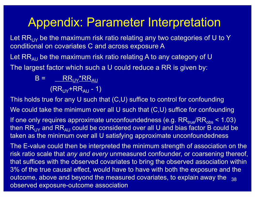
Appendix: Parameter InterpretationLet RRUY be the maximum risk ratio relating any two categories of U to Y conditional on covariates C and across exposure ALet RRAU be the maximum risk ratio relating A to any category of UThe largest factor which such a U could reduce a RR is given by:

B = RRUY*RRAU

(RRUY+RRAU - 1)This holds true for any U such that (C,U) suffice to control for confoundingWe could take the minimum over all U such that (C,U) suffice for confoundingIf one only requires approximate unconfoundedness (e.g. RRtrue/RRobs < 1.03) then RRUY and RRAU could be considered over all U and bias factor B could be taken as the minimum over all U satisfying approximate unconfoundednessThe E-value could then be interpreted the minimum strength of association on the risk ratio scale that any and every unmeasured confounder, or coarsening thereof, that suffices with the observed covariates to bring the observed association within 3% of the true causal effect, would have to have with both the exposure and the outcome, above and beyond the measured covariates, to explain away the observed exposure-outcome association

38

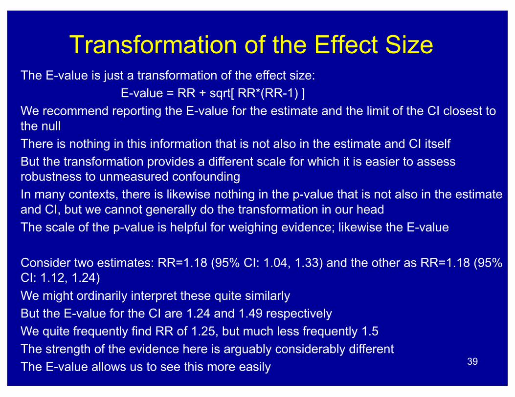
Transformation of the Effect SizeThe E-value is just a transformation of the effect size:

E-value = RR + sqrt[ RR*(RR-1) ]We recommend reporting the E-value for the estimate and the limit of the CI closest to the nullThere is nothing in this information that is not also in the estimate and CI itselfBut the transformation provides a different scale for which it is easier to assess robustness to unmeasured confoundingIn many contexts, there is likewise nothing in the p-value that is not also in the estimate and CI, but we cannot generally do the transformation in our headThe scale of the p-value is helpful for weighing evidence; likewise the E-value

Consider two estimates: RR=1.18 (95% CI: 1.04, 1.33) and the other as RR=1.18 (95% CI: 1.12, 1.24)We might ordinarily interpret these quite similarlyBut the E-value for the CI are 1.24 and 1.49 respectivelyWe quite frequently find RR of 1.25, but much less frequently 1.5The strength of the evidence here is arguably considerably differentThe E-value allows us to see this more easily 39

Relation to Rosenbaum’s Design Sensitivity

The E-value bears some relation to Rosenbaum’s “design sensitivity” (Rosenbaum, 2004) but…

(1) Design sensitivity focuses on much how the odds of treatment of two units with identical covariates may differ, rather than relations with the outcome; the sensitivity analysis “amplification” (Rosenbaum and Silber, 2009) considers the relation with the outcome but under parametric models rather than non-parametrically

(2) Design sensitivity provides sensitivity to unmeasured confounding for infinite samples, rather than the actual sample

(3) Design sensitivity uses odds ratio scales, which can vastly exaggerate risk ratios and hence the intuitive understanding of robustness of results

40

Inference With and Using the E-valueOne could calculate the confidence interval for the E-value for the confounded association but this would give statements like:

“Across repeated samples, at least 95% of the time, the minimum strength of association on the risk ratio scale that an unmeasured confounder would have to have with both the exposure and the outcome, conditional on the measured covariates, to explain away the actual confounded exposure-outcome association will lie in the confidence interval provided.”

If instead we calculate the E-value for the lower limit of the confidence interval we can make statements of the form:

“Across repeated samples, at least 95% of the time, if the actual confounding parameters RRUY and RREU are both less than the E-value for the confidence interval that was calculated, then there will be a true effect in the same direction as the observed association”

The object of inference is arguably the causal effect itself, not the E-value; the E-value is just a tool; statements of the latter type are arguably generally of greater interest

41

Sensitivity Analysis w/o Assumptions

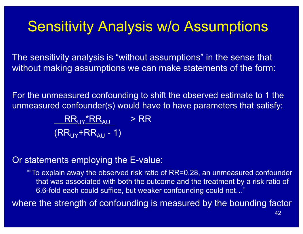
The sensitivity analysis is “without assumptions” in the sense that without making assumptions we can make statements of the form:

For the unmeasured confounding to shift the observed estimate to 1 the unmeasured confounder(s) would have to have parameters that satisfy:

RRUY*RRAU > RR(RRUY+RRAU - 1)

Or statements employing the E-value:““To explain away the observed risk ratio of RR=0.28, an unmeasured confounder

that was associated with both the outcome and the treatment by a risk ratio of 6.6-fold each could suffice, but weaker confounding could not…”

where the strength of confounding is measured by the bounding factor42

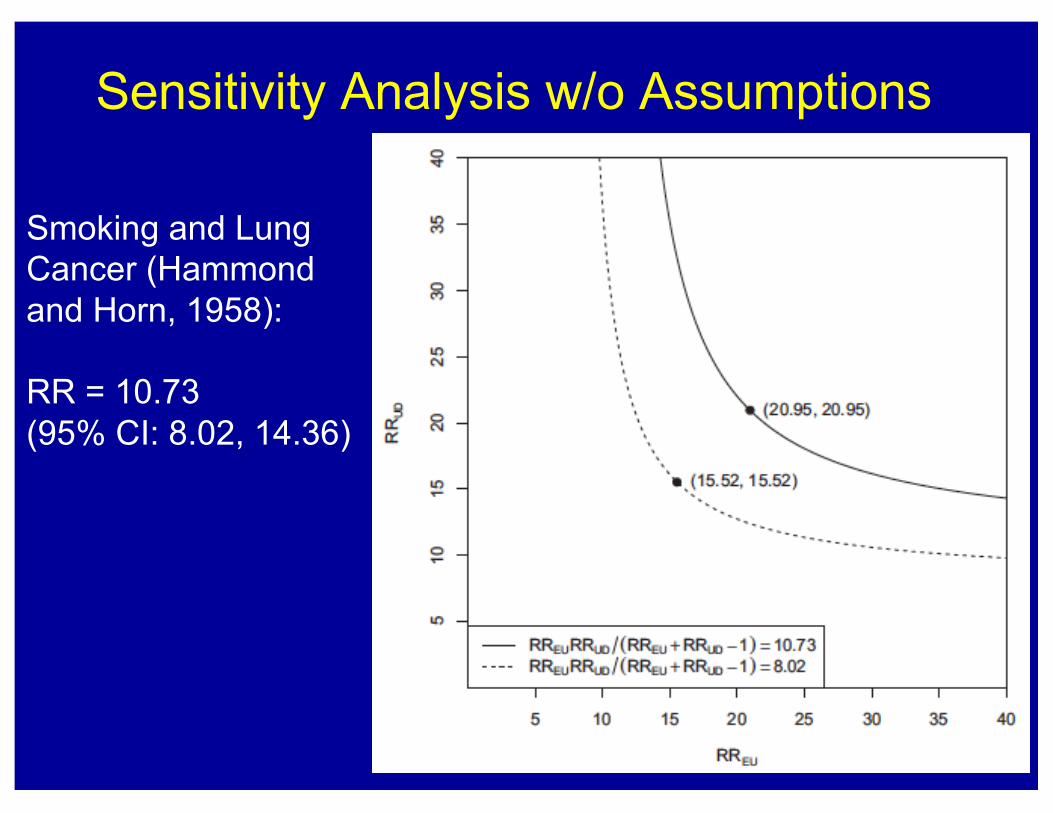
Sensitivity Analysis w/o Assumptions

Smoking and Lung Cancer (Hammond and Horn, 1958):

RR = 10.73 (95% CI: 8.02, 14.36)

43