Sensitivity analysis for the control of oblique shock

wave/laminar boundary layer interactions at Mach 5.92

Nathaniel Hildebrand∗, Anubhav Dwivedi∗, Joseph W. Nichols†, and Graham V. Candler‡

University of Minnesota, Minneapolis, MN, 55455, USA

Mihailo R. Jovanovic§

University of Southern California, Los Angeles, CA, 90089, USA

At a transitional Reynolds number, we examine the instability of an oblique shockwave impinging on a hypersonic laminar boundary layer. Using global stability analysiswe identify the critical oblique shock angle at which the 2D laminar flow first becomesunstable to 3D perturbations. The non-dimensional spanwise wavenumber selected at thisbifurcation is β = 0.25. Long streamwise streaks that originate in the shear layer on top ofthe recirculation bubble are present in the unstable stationary global mode. We computethe adjoint eigenmodes to understand how upstream fluctuations affect the direct globalmodes of the system, and we see that the least stable stationary global mode is receptive toforcing inside the boundary layer and along the oblique shock wave. The wavemaker, whichis defined as the sensitivity of an eigenvalue to base flow modification, is then computed.For every case, the wavemaker resides in the recirculation bubble, but it shifts towardsthe reattachment point as the incident shock angle increases. A calculation of the Gortlernumber about several 2D base flows revealed that a centrifugal instability cannot be thesole reason for bifurcation.

I. Introduction

High-speed flows over complex geometries are typically characterized by shock wave/boundary layerinteractions (SWBLI) and have been the subject of many experimental and numerical investigations.1 Thestrong adverse pressure gradient created by an oblique shock wave impinging on a laminar boundary layercan cause it to separate from the wall. Boundary layer separation results in the formation of a recirculationbubble that can become three-dimensional (3D) and unsteady. Thus, SWBLI provides a mechanism fortransition to turbulence that is different from the usual pathways based on boundary layer instabilitiesinitiated by Mack modes.2,3 Once a hypersonic boundary layer has transitioned, the skin friction and heatflux increase by a factor of five to six.4 Additionally, in the case of SWBLI, self-sustained oscillationssupported by the recirculation bubble may produce unsteady loads.

The interaction of a laminar boundary layer with shock waves has been studied using stability theoryand numerical simulations at subsonic and supersonic conditions. For an incompressible separation bubble,Theofilis et al.5 and Rodriguez & Theofilis6 determined that a region of positive skin-friction inside theprimary bubble results in a bifurcation from two-dimensional (2D) flow to a 3D steady state. Robinet7 useddirect numerical simulations (DNS) of a compressible SWBLI to show that a steady 2D flow bifurcates toa 3D state in different ways as the oblique shock angle increases depending on the spanwise extent of thecomputational domain. For small spanwise domain sizes, the SWBLI bifurcated into a steady 3D flow withan increase in the shock angle. As the oblique shock angle increases yet further, the flow bifurcated into anunsteady 3D state. For sufficiently large spanwise extents, however, the 2D flow bifurcated directly to a 3D

∗Graduate Research Assistant, UMN Aerospace Engineering and Mechanics, AIAA Student Member.†Assistant Professor, UMN Aerospace Engineering and Mechanics, AIAA Member.‡Russell J. Penrose and McKnight Presidential Professor, UMN Aerospace Engineering and Mechanics, AIAA Fellow.§Professor, USC Electrical Engineering, IEEE Senior Member.

1 of 14

American Institute of Aeronautics and Astronautics

Dow

nloa

ded

by U

NIV

ER

SIT

Y O

F M

INN

ESO

TA

on

Sept

embe

r 30

, 201

7 | h

ttp://

arc.

aiaa

.org

| D

OI:

10.

2514

/6.2

017-

4312

47th AIAA Fluid Dynamics Conference

5-9 June 2017, Denver, Colorado

AIAA 2017-4312

Copyright © 2017 by the American Institute of Aeronautics and Astronautics, Inc.

All rights reserved.

AIAA AVIATION Forum

unsteady state. Global stability analysis identified an unstable stationary mode, which explained the firstbifurcation to a steady 3D flow.

There are currently two explanations for the source of low-frequency unsteadiness in an oblique shockwave/turbulent boundary layer interaction. On one hand, several studies show how shock motion is linked tothe turbulence of an incoming boundary layer. Although not directly related to low-frequency unsteadiness,Erengil & Dolling8 convey in their experimental work on compression ramps at Mach 5 how small-scalejittery motion of the shock wave is affected by the passage of fluctuations in static quantities across it.Unalmis & Dolling9 propose low-frequency unsteadiness is influenced by the thickening and thinning of theturbulent boundary layer upstream. More recently, Ganapathisubramani et al.10 show in their experimentalstudies that shock motion is affected by long upstream low-speed and high-speed streaks. Wu & Martin11

saw a significant correlation between motion of the separation line surrogate and fluctuations in the upstreamboundary layer with DNS. This agrees well with previous work.10 However, the correlation was lower whentested with the actual separation line. In the large eddy simulations of Touber & Sandham,12 low-frequencyoscillations are observed when no coherent structures exist upstream. Nichols et al.14 show that turbulentSBLI can be interpreted as a forced weakly damped oscillator. Lastly, Priebe & Martin13 suggest thatGortler instability is important for turbulent boundary layers over a compression ramp.

An extensive amount of work suggests the internal mechanism within the recirculation bubble is responsi-ble for the unsteadiness. Dupont et al.15 points to coherence between wall pressure fluctuations at the foot ofthe reflected shock and in the reattachment zone for a turbulent SWBLI. This corresponds to the breathingcharacter of the separation bubble. A simple model based on entrainment characteristics of the shear layeras well as the mass recharge within the separation bubble has been proposed.16 This model describes theunsteady motion of the reattachment point. Pirozzoli & Grasso17 developed an alternative mechanism forunsteadiness driven by resonance, which involves the interaction of large structures with the incident shock.They thought this would produce acoustic disturbances that travel upstream to the separation point andlead to the low-frequency motion of the reflected shock. Studies by Touber & Sandham12 as well as Sansicaet al.18 show there is no need for upstream forcing to obtain an unsteady response. However, they also revealthat upstream disturbances do provide a broad source of unsteady low-frequency motion. In a recent review,Clemens & Narayanaswamy19 argue the upstream and internal mechanism are always active independent ofthe interaction strength.

Literature related to an oblique shock wave impinging on a laminar boundary layer at hypersonic speedsis sparse. Benay et al.20 performed a study of SWBLI in a hollow cylinder flare model at Mach 5. Alocal linear stability analysis complemented this experimental and numerical investigation. For this flowconfiguration, oblique modes are the most unstable. More recently, Sandham et al.21 carried out a numericaland experimental study on SWBLI at Mach 6. It is suggested that the transition process develops from secondor Mack mode instabilities superimposed on streamwise streaks.

Our focus in this work is to more closely examine the bifurcation of an initially 2D flow to a 3D steadystate that occurs for an oblique shock wave/laminar boundary layer interaction at Mach 5.92. The spanwisewavenumber selected at this bifurcation is characterized with global stability analysis about 2D base flows.The US3D hypersonic flow solver22 is used to calculate the steady base flows. We compute the adjointeigenmodes to understand how upstream fluctuations affect the direct global modes of the system. This canhelp explain the impact of turbulence on a SWBLI and the global modes specifically. The sensitivity of aneigenvalue to base flow modification or the wavemaker is calculated using direct and adjoint information.This reveals the spatial origin of the stability modes. We compute the Gortler number associated with curvedstreamlines taken from the DNS base flows to assess the possibility of centrifugal instability.13

II. Problem formulation

A. Flow configuration

We consider an oblique shock wave/laminar boundary layer interaction for this study. The flow configurationis depicted in Figure 1. We set the freestream Mach number, temperature, and pressure to the values ofM∞ = 5.92, T∞ = 53.06 K, and p∞ = 308.2 Pa, respectively. These values exactly match experimentsperformed in the ACE Hypersonic Wind Tunnel at Texas A&M University.23 We use a Reynolds number ofRe = ρ∞U∞δ

∗/µ∞ = 9660, based on the undisturbed boundary layer displacement thickness δ∗ at the inlet.This corresponds to a unit Reynolds number of 4.6 × 106 m−1 close to transition. Here, ρ∞, U∞, and µ∞denote the freestream density, velocity, and dynamic viscosity, respectively. Note that the freestream values

2 of 14

American Institute of Aeronautics and Astronautics

Dow

nloa

ded

by U

NIV

ER

SIT

Y O

F M

INN

ESO

TA

on

Sept

embe

r 30

, 201

7 | h

ttp://

arc.

aiaa

.org

| D

OI:

10.

2514

/6.2

017-

4312

are taken upstream of the bow shock and the incident shock. To enable a comprehensive analysis aboutthe stability of this flow field, we simulate a range of incident shock angles θ from 12 to 13.4 degrees. Weutilize a Cartesian coordinate system in this study with x, y, and z denoting the streamwise, wall-normal,and spanwise directions, respectively.

Figure 1: A detailed schematic adapted from Robinet7 of our 2D computational domain. HereLsep and Lint denote the separation and interaction lengths, respectively.

B. Governing equations

The compressible Navier-Stokes equations are used to mathematically model the dynamics of an oblique shockwave/laminar boundary layer interaction at hypersonic speeds. These equations govern the evolution of thesystem state q = [p; uT; s]T, where p, u, and s are the fluid pressure, velocity, and entropy, respectively.24,25

After non-dimensionalization with respect to the displacement thickness δ∗, freestream velocity U∞, densityρ∞, and temperature T∞, these equations are

∂p

∂t+ u · ∇p+ ρc2∇ · u =

1

Re

[1

M2∞Pr∇ · (µ∇T ) + (γ − 1)φ

], (1a)

∂u

∂t+

1

ρ∇p+ u · ∇u =

1

Re

1

ρ∇ · τ, (1b)

∂s

∂t+ u · ∇s =

1

Re

1

ρT

[1

(γ − 1)M2∞Pr∇ · (µ∇T ) + φ

]. (1c)

For an ideal fluid, the density ρ and temperature T are related to pressure p through the equation of stateγM2∞p = ρT . We define the Mach number M∞ = U∞/c∞, where c∞ =

√γp∞/ρ∞ is the speed of sound in

the freestream. Further, γ = 1.4 is the assumed constant ratio of specific heats.We define entropy as s = ln(T )/[(γ − 1)M2

∞]− ln(p)/(γM2∞) so that s = 0 when p = 1 and T = 1. The

viscous stress tensor τ can be written in terms of the identity matrix I, velocity vector u, and dynamicviscosity µ to yield the following expression

τ = µ[∇u+ (∇u)T − 2

3(∇ · u)I]. (2)

The viscous dissipation is defined as φ = τ : ∇u. Note the operator : represents a scalar or double dotproduct between two tensors. We set λ/µ = −2/3 with λ denoting the second viscosity coefficient. In orderto compute the dynamic viscosity µ, we used Sutherland’s law with Ts = 110.3 K as follows

µ(T ) = T 3/2 1 + Ts/T∞T + Ts/T∞

. (3)

3 of 14

American Institute of Aeronautics and Astronautics

Dow

nloa

ded

by U

NIV

ER

SIT

Y O

F M

INN

ESO

TA

on

Sept

embe

r 30

, 201

7 | h

ttp://

arc.

aiaa

.org

| D

OI:

10.

2514

/6.2

017-

4312

The Prandtl number is set to a constant value Pr = µ(T )/κ(T ) = 0.72, where κ(T ) is the coefficient of heatconductivity. We can recast system (1) into the form ∂q/∂t = F (q), where F is the differential non-linearNavier-Stokes operator.

C. Linearized model

To investigate the behavior of small fluctuations about various base flows, we linearize system (1) by decom-posing the state variables q = q+q′ into steady and fluctuating parts. By keeping only the first-order termsin q′, we arrive at the linearized Navier-Stokes equations

∂p′

∂t+ u · ∇p′ + u′ · ∇p + ρc2∇ · u′ + γ(∇ · u)p′ =

1

Re

{1

M2∞Pr∇ · (µ∇T ′)

+ (γ − 1)[τ :∇u′ + τ′ :∇u

]},

(4a)

∂u′

∂t+

1

ρ∇p′ − ρ′

ρ2∇p+ u · ∇u′ + u′ · ∇u =

1

Re

{1

ρ∇ · τ′ − ρ′

ρ2∇ · τ

}, (4b)

∂s′

∂t+ u · ∇s′ + u′ · ∇s =

1

Re

1

ρT

{1

(γ − 1)M2∞Pr

[∇ · (µ∇T ′)− p′

p∇ · (µ∇T )

]+ τ :∇u′ + τ′ :∇u− p′

pτ :∇u

}.

(4c)

Here the overbars and primes denote the base flow and fluctuating parts, respectively. We linearize theequation of state to obtain ρ′/ρ = p′/p − T ′/T . The expression T ′ = (γ − 1)M2

∞(T s′ + p′/ρ) comes fromlinearizing the definition of entropy and substituting in the equation of state. We neglect fluctuations in thedynamic viscosity or set µ′ = 0. This assumption is reasonable due to the fact that µ′ is significantly smallerthan the other fluctuating quantities.

Global modes of the linear system (4) take the form

q′(x, y, z, t) = q(x, y)ei(βz−ωt), (5)

where β is the non-dimensional spanwise wavenumber and ω is the temporal frequency. We can representsystem (4) abstractly as equation (6a). Furthermore, the Jacobian operator given by A = ∂F/∂q|q cor-responds to the linearization of the Navier-Stokes operator F about the base flow q. Now an eigenvalueproblem of the form Aq = −iωq can be solved numerically.

In addition to the eigenvalues and their associated eigenfunctions, we are also interested in their sen-sitivity to slight changes in the base flow.26 We define the spatial region of maximum sensitivity as thewavemaker27,28 because it corresponds to the location where an instability originates. The wavemaker canbe computed after solving the adjoint problem. If q+ represents the adjoint state variables, and we defineA+ as the adjoint of operator A, then we arrive at system (6b). Notice the equations below are similar

∂q′

∂t= Aq′,

∂q+

∂t= A+q+. (6a,b)

Thus, the direct and adjoint problems can be solved in an identical manner. Eigenvalue spectra computedwith the direct and adjoint equations should be conjugate symmetric by construction. The correspondingeigenfunctions are expected to be significantly different. As we will see later, the adjoint perturbationstravel upstream instead of downstream with the flow. We calculated the adjoint operator A+ by applyingintegration by parts to system (4).

4 of 14

American Institute of Aeronautics and Astronautics

Dow

nloa

ded

by U

NIV

ER

SIT

Y O

F M

INN

ESO

TA

on

Sept

embe

r 30

, 201

7 | h

ttp://

arc.

aiaa

.org

| D

OI:

10.

2514

/6.2

017-

4312

D. Numerical methods

For the base flow calculations, we solve the compressible Navier-Stokes equations in conservative form.29

A stable low-dissipation scheme based upon the kinetic energy consistent (KEC) method developed bySubbareddy and Candler30 is implemented for the inviscid flux computation. In this numerical method, wesplit the inviscid flux into a symmetric (or non-dissipative) portion and an upwind (or dissipative) portion.We premultiply the flux by a shock-detecting switch, which ensures that the dissipation only occurs aroundshocks.31 A fourth-order centered KEC scheme is employed for the present study. The viscous fluxes aremodeled with central differences that have second-order accuracy. We perform time integration using animplicit second-order Euler method with point relaxation to maintain numerical stability.32

The linear system of equations (4) are discretized by fourth-order centered finite differences applied on astretched mesh. This results in a large sparse matrix.25 Global modes are extracted by the shift-and-invertArnoldi method as implemented by the software package ARPACK.33 The inversion step is computed byfinding the LU decomposition of the shifted sparse matrix using the massively parallel SuperLU package.34

We used a numerical filter to add minor amounts of scale-selective artificial dissipation to damp spuriousmodes associated with the smallest wavelengths allowed by the mesh. This filter does not affect the discretemodes of interest if they are well-resolved.35 The numerical filter is introduced by adding terms of the formε(∂4q/∂x4) and ε(∂4q/∂y4). Sponge layers are employed at the top, left, and right boundaries to absorboutgoing information with minimal reflection.36

III. RESULTS

A. Base flows

In order to conduct a detailed analysis of an oblique shock wave/laminar boundary layer interaction at Mach5.92, we first need to compute several steady 2D base flows. The only parameter that changes across thesebase flows is the incident shock angle. We first obtain the boundary condition without the incident shockat the left inlet separately for this SWBLI by simulating a zero-pressure-gradient boundary layer developingover a flat plate.29 Next, we introduce the incident oblique shock wave by enforcing the Rankine-Hugoniotconditions at a point along the left boundary. We select this point so that the oblique shock impinges uponthe wall at a fixed distance of 119δ∗ from the leading edge. This ensures that the Reynolds number at theimpingement point is constant for various shock angles. The bottom boundary is modeled as an adiabaticwall. We enforce a hypersonic freestream inlet along the top boundary. Lastly, we impose an outlet boundarycondition along the right edge of the domain.

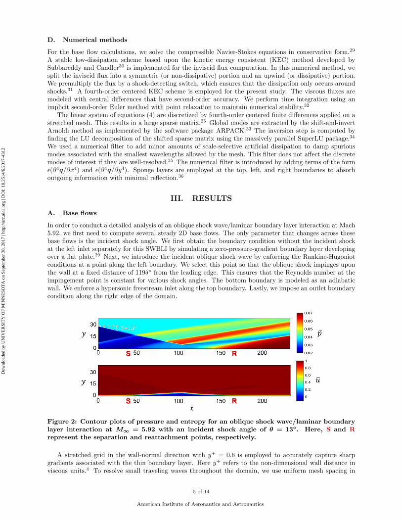
Figure 2: Contour plots of pressure and entropy for an oblique shock wave/laminar boundarylayer interaction at M∞ = 5.92 with an incident shock angle of θ = 13◦. Here, S and Rrepresent the separation and reattachment points, respectively.

A stretched grid in the wall-normal direction with y+ = 0.6 is employed to accurately capture sharpgradients associated with the thin boundary layer. Here y+ refers to the non-dimensional wall distance inviscous units.4 To resolve small traveling waves throughout the domain, we use uniform mesh spacing in

5 of 14

American Institute of Aeronautics and Astronautics

Dow

nloa

ded

by U

NIV

ER

SIT

Y O

F M

INN

ESO

TA

on

Sept

embe

r 30

, 201

7 | h

ttp://

arc.

aiaa

.org

| D

OI:

10.

2514

/6.2

017-

4312

the streamwise direction. At a single frequency, long wavelengths in the freestream are connected to shortwavelengths inside the recirculation bubble because of the large velocity difference. We resolved the domainby nx = 998 and ny = 450 grid points in the streamwise and wall-normal directions, respectively. Thisresolution is sufficient according to a recent grid convergence study.29

We ran the base flow simulations for approximately sixty flow through times with the US3D hypersonicflow solver,22 until the residual was on the order of machine zero. A base flow with θ = 13◦ is shown inFigure 2. We non-dimensionalize x, y, and z by the displacement thickness δ∗. Notice the presence ofan incident shock, a bow shock, compression waves, and an expansion fan in the pressure contours. Weclearly see how the boundary layer develops in the streamwise velocity contours. This case is unstable to 3Dfluctuations, which we will see later. It is, however, stable for fluctuations with a spanwise wavenumber ofβ = 0. Therefore, by enforcing two-dimensionality upon our simulations, we can converge to an exact steadystate solution to the base flow equations (1) that is unstable to small fluctuations.

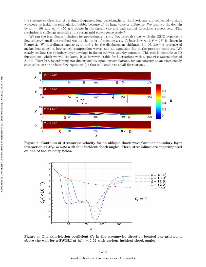
Figure 3: Contours of streamwise velocity for an oblique shock wave/laminar boundary layerinteraction at M∞ = 5.92 with four incident shock angles. Here, streamlines are superimposedon one of the velocity fields.

Figure 4: The skin-friction coefficient Cf in the streamwise direction located one grid pointabove the wall for a SWBLI at M∞ = 5.92 with various incident shock angles.

6 of 14

American Institute of Aeronautics and Astronautics

Dow

nloa

ded

by U

NIV

ER

SIT

Y O

F M

INN

ESO

TA

on

Sept

embe

r 30

, 201

7 | h

ttp://

arc.

aiaa

.org

| D

OI:

10.

2514

/6.2

017-

4312

To visualize how the SWBLI changes with the incident shock angle, we plot contours of streamwisevelocity for several base flows in Figure 3. The recirculation bubble gets significantly larger as the incidentshock angle increases from 12◦ to 13.4◦. Here Lsep = 74 for θ = 12◦ and Lsep = 126 for θ = 13.4◦, whereeach quantity has been non-dimensionalized by the displacement thickness δ∗. The recirculation bubble alsobecomes less symmetric as the incident shock angle increases.

Figure 4 shows the wall skin-friction coefficient for a range of incident shock angles from 12◦ to 13.4◦.Notice that the skin-friction coefficient is entirely positive inside the bubble. This is not always the case asshown in Theofilis et al.5 for an incompressible regime. It is suggested in Rodriguez & Theofilis6 that thepresence of a secondary bubble, or negative wall skin-friction coefficient, inside the primary bubble leads toa bifurcation of the flow to a 3D steady state. We will focus our attention on incident shock angles θ ≤ 13.4◦

and find that in the compressible regime this bifurcation occurs well before a secondary bubble forms. Here,the streamwise length of the recirculation bubble increases almost linearly with the oblique shock angle.37

B. Global mode analysis

To determine the critical incident shock angle at which the flow first becomes unstable, we apply globalstability analysis over a range of shock angles and spanwise wavenumbers. For example, Figure 5 showsan eigenvalue spectrum resulting from global mode analysis with a shock angle of θ = 13◦ at a spanwisewavenumber β = 0.1. Frequencies are expressed in non-dimensional form as Strouhal numbers defined asSt = fδ∗/U∞ for this study. The real and imaginary parts of the complex frequency St = Str + iSti denotethe temporal frequency and growth rate, respectively.

In the shift-and-invert Arnoldi method33 used to compute the eigenvalue spectrum, shifts are positionedalong the real axis to capture the least stable modes. Twenty eigenvalues are converged at each shift. Wespaced shifts close together so that a portion of the spectrum converged at each shift partially overlaps with aportion converged at neighboring shifts. Modes corresponding to redundant eigenvalues extracted by nearbyshifts agree well with one another, providing one check of the Arnoldi method. More eigenvalues can befound using additional shifts or increasing the number of eigenvalues sought at each shift.

Figure 5: The eigenvalue spectrum of a SWBLI at M∞ = 5.92 with an incident shock angleof θ = 13◦ and spanwise wavenumber β = 0.1.

Every eigenvalue in Figure 5 has a negative growth rate, which means the system is globally stable. Figure6 displays two eigenmodes and the position of three sponge layers. Mode 1 corresponds to the least stablezero frequency eigenvalue. Notice that a significant portion of the perturbation lies within the recirculationbubble for this stationary global mode. We also see a streamwise streak that extends downstream until itgets driven to zero by the right sponge layer. Mode 2, which corresponds to an oscillatory eigenvalue, hasa lot of structure within the recirculation bubble. Notice that the real streamwise velocity perturbation inglobal mode 2 contains positive and negative components near the front portion of the bubble. This modeis structurally similar to the other surrounding oscillatory eigenmodes (not shown). For both global modes,

7 of 14

American Institute of Aeronautics and Astronautics

Dow

nloa

ded

by U

NIV

ER

SIT

Y O

F M

INN

ESO

TA

on

Sept

embe

r 30

, 201

7 | h

ttp://

arc.

aiaa

.org

| D

OI:

10.

2514

/6.2

017-

4312

the long streamwise streak appears to originate near the apex of the recirculation bubble. There is also asmall amount of the perturbation that surrounds a few shock waves.

Figure 6: Stable global modes labeled in Figure 5 colored by the real part of the streamwisevelocity perturbation. Here, the dashed lines indicate the start of three different sponge layers.

Next, we increase the spanwise wavenumber to β = 0.25 and repeat the same analysis, keeping theshock angle fixed at θ = 13◦. Figure 7 shows the eigenvalue spectrum at these conditions. We see that onestationary eigenmode has a positive growth rate, which means the system is globally unstable. Robinet7

found a similar unstable stationary mode for an oblique shock wave/laminar boundary layer interaction atMach 2.15. Figure 8 displays the least stable zero frequency eigenmode in 3D. This unstable global modealso contains long streamwise streaks similar to those shown in Figure 6 at a lower spanwise wavenumber.These elongated structures are still clearly coupled to the shear layer on top of the recirculation bubble.Finally, repeating global stability analysis for a spanwise wavenumber β = 0.5, we find that the eigenvaluespectrum becomes globally stable again.

Figure 7: The eigenvalue spectrum of a SWBLI at M∞ = 5.92 with an incident shock angleof θ = 13◦ and spanwise wavenumber β = 0.25.

While θ = 13◦ supported global instability over a range of spanwise wavenumbers, stability analysisof incident shock angles θ = 12.6◦ and θ = 12.8◦ revealed these cases to be globally stable at all spanwisewavenumbers. Increasing the shock angle to θcrit = 12.9◦, however, resulted in instability at a single spanwise

8 of 14

American Institute of Aeronautics and Astronautics

Dow

nloa

ded

by U

NIV

ER

SIT

Y O

F M

INN

ESO

TA

on

Sept

embe

r 30

, 201

7 | h

ttp://

arc.

aiaa

.org

| D

OI:

10.

2514

/6.2

017-

4312

wavenumber βcrit = 0.25. Figure 9 shows the maximum growth rate versus spanwise wavenumber for anglesranging from θ = 12.6◦ to θ = 13◦. Above the critical shock angle θcrit = 12.9◦, the 2D flow bifurcates toa 3D steady state with spanwise wavenumber βcrit = 0.25. The least stable global mode for every incidentshock angle and spanwise wavenumber is zero frequency. Thus, the flow will never become unsteady at theseconditions. We see that β = 0.25 results in the largest growth rate for every shock angle. As the spanwisewavenumber approaches zero, we expect the system to become fully stable because the base flows are 2Dand the 3D component of the perturbation gets smaller. The system stabilizes for spanwise wavenumbersabove β = 0.5, which has been seen before.6,7

Figure 8: The unstable global mode, or more specifically qei(0.25z) +c.c., in Figure 7 visualizedby the real part of the normalized, non-dimensional streamwise velocity perturbation. Reddenotes a positive velocity while blue is negative.

Figure 9: The maximum growth rate versus spanwise wavenumber for an oblique shockwave/laminar boundary layer interaction at M∞ = 5.92 with four incident shock angles.

C. Sensitivity analysis

In the previous section, we found that the 2D oblique shock wave/boundary layer interaction bifurcates toa 3D steady state at θ = 12.9◦. To further interpret the physical mechanism responsible for bifurcation, we

9 of 14

American Institute of Aeronautics and Astronautics

Dow

nloa

ded

by U

NIV

ER

SIT

Y O

F M

INN

ESO

TA

on

Sept

embe

r 30

, 201

7 | h

ttp://

arc.

aiaa

.org

| D

OI:

10.

2514

/6.2

017-

4312

consider the sensitivity of the unstable mode to base flow modification. This also allows us to assess therobustness of our results and to understand the spatial origin of the stability modes.

First, we compute the adjoint modes to study how upstream fluctuations affect the direct global modesof the SWBLI. An adjoint eigenmode indicates where the flow is most receptive to forcing.28 We solvethe adjoint system (6b) with the continuous approach. Here integration by parts is used to derive theequations, which are then discretized. This allows for proper incorporation of the boundary conditions.Adjoint modes also allow us to quantify sensitivity of an eigenspectrum to changes in the base flow. Weconsider the shock angle θ = 13◦ with spanwise wavenumber β = 0.25 initially. Moreover, the stretched gridwith (nx, ny) = (998, 450) was again employed for this analysis. Figure 10 illustrates the unstable adjointglobal mode that corresponds to the direct mode shown in Figure 8 with contours of streamwise velocityperturbation. The spatial separation of the direct and adjoint global modes shown in Figures 8 and 10indicate significant convective non-normality. For a comprehensive discussion on non-normal operators andtheir properties see Schmid and Henningson.38

Figure 10: The unstable global mode, or more specifically q+ei(0.25z) + c.c., in Figure 7 visu-alized by the real part of the normalized, non-dimensional streamwise velocity perturbation.Red denotes a positive velocity while blue is negative.

Notice that in Figure 10 long streaks are present inside the boundary layer extending from the inletdownstream to the recirculation bubble. There is also a component of the perturbation that resides alongthe incident shock in the freestream. This means that the unstable eigenmode is receptive to forcing in theboundary layer and around the incident shock. We do not show the adjoint eigenvalue spectrum because itis exactly conjugate symmetric to the direct eigenvalue spectrum in Figure 7. If the grid size is adequate toresolve the small scales, then we know that the continuous adjoint and direct eigenspectra will be conjugatesymmetric.27 We see similar results for the stable global modes at θ = 13◦ and β = 0.25 as well as withmodes at other incident shock angles and spanwise wavenumbers not shown here.

Mathematically, an upper bound for the deviation of an eigenvalue ∂ωj associated with the linear operatorA due to a structural perturbation P (such as that created by changing the base flow slightly) is given by|∂ωj | ≤ ||q′j ||E ||P ||E‖|q

+j ||E from Schmid and Henningson.38 Here q′j and q+

j are the direct and adjointeigenmodes corresponding to the deviation ∂ωj , respectively. The subscript E denotes an energy normbased on the standard definition of weighted norms.39 Here, P has the strongest effect when ||q′j ||E ||q

+j ||E

is large. In physical terms, this is the region of space where the direct and adjoint global modes overlap.28

An eigenvalue is generally insensitive to modifications of the base flow outside this region. Therefore, wedefine the wavemaker as ||q′j ||E ||q

+j ||E , since this quantity provides an upper boundary on the sensitivity of

an eigenvalue to base flow modification.27

We show the wavemaker for incident shock angles ranging from θ = 12◦ to θ = 13.4◦ in Figure 11. Wehold the spanwise wavenumber to a constant value of 0.25. Notice that for every case the wavemaker islocated far away from the top, left, and right boundary. Therefore, any changes to the three sponge layers ordomain size should not have a significant impact on the global mode dynamics. For an incident shock angleof θ = 12◦, we see that the wavemaker resides in the recirculation bubble. It is evenly distributed between the

10 of 14

American Institute of Aeronautics and Astronautics

Dow

nloa

ded

by U

NIV

ER

SIT

Y O

F M

INN

ESO

TA

on

Sept

embe

r 30

, 201

7 | h

ttp://

arc.

aiaa

.org

| D

OI:

10.

2514

/6.2

017-

4312

separation and reattachment points. As the shock angle increases to θ = 13.4◦, we see the wavemaker shiftto the back portion of the recirculation bubble near reattachment. This behavior is directly connected to thechange in symmetry of the recirculation bubble seen in Figure 3. Therefore, the bifurcation at θ = 12.9◦ islikely a product of the recirculation bubble and wavemaker being skewed toward reattachment. Rememberthat streamlines close to the recirculation bubble have significantly more curvature over the back portionthan over the front for θ ≥ 12.9◦. The wavemaker is similar for the other relevant global modes at differentincident shock angles and spanwise wavenumbers. One can use structural sensitivity analysis to understandhow to optimally modify the base flow inside the wavemaker to alter the stability characteristics of an obliqueshock wave/laminar boundary layer interaction, but this is left to a future study.

Figure 11: The wavemaker for an oblique shock wave/laminar boundary layer interaction withfour incident shock angles. Every case is associated with the least stable global mode at aspanwise wavenumber of β = 0.25. A dividing streamline is superimposed on each case.

D. Gortler instability

Since the global mode shapes and base flow sensitivity analysis indicate the importance of regions in the flowwhere streamlines have significant curvature, we investigate Gortler instability40 as a possible mechanismdriving the bifurcation. Long streamwise streaks seen in Figures 6 and 8 also suggest the presence of Gortlervortices. To quantify this effect, we define the radius of curvature for streamlines with the expression below.41

R =‖u‖

∇ψ · (u · ∇u)(7)

Here, ‖u‖ represents the Euclidean norm of the base flow velocity, and ψ is the streamfunction such thatu =∇×ψ where ψ = [0 0 ψ]. We express the streamline curvature as κ = ε(x/δ∗)/R with ε denoting theviscous scale.42 In this study, we define the Gortler number as

G =√κ/ε. (8)

Figure 12 shows the Gortler number G as a function of streamwise location evaluated from base flows withθ = 12◦, θ = 12.6◦, θ = 13◦, and θ = 13.4◦. This is applied to the streamline with a wall-normal distance of1.5δ∗ at the inlet. For compressible flow, Gortler vortices likely become important when G > 0.6 accordingto Hall & Malik.43 Notice in Figure 12 that the Gortler number surpasses this critical value near separationand reattachment in every base flow.

We see for θ = 12◦ that the Gortler number is equally large upstream and downstream of the recirculationbubble. As the incident shock angle grows, the Gortler number decreases at the separation point andincreases near reattachment. This is expected because the curvature of streamlines along the back portion

11 of 14

American Institute of Aeronautics and Astronautics

Dow

nloa

ded

by U

NIV

ER

SIT

Y O

F M

INN

ESO

TA

on

Sept

embe

r 30

, 201

7 | h

ttp://

arc.

aiaa

.org

| D

OI:

10.

2514

/6.2

017-

4312

of the recirculation bubble increases with growing shock angle. The largest value of G is roughly 1.9, whichhappens near the reattachment point for θ = 13.4◦. Furthermore, there is a clear relationship between theasymmetry of the recirculation bubble, the position of the wavemaker, and the Gortler number. We do knowthat centrifugal instability is responsible for amplifying the streamwise streaks in the SWBLI. Since theGortler number surpasses its critical value for base flows with an incident shock angle less than θ = 12.9◦,however, we know that Gortler instability cannot be solely responsible for the bifurcation. The formation ofstreamwise streaks at all shock angles, even though they are temporally damped, gives further evidence tothis conclusion.

Figure 12: Plots of Gortler number versus streamwise location for several 2D base flows. Weonly display G when the streamlines are concave.

IV. CONCLUSIONS

An oblique shock wave impinging on a laminar boundary layer at Mach 5.92 has been investigated. Wecomputed 2D base flows with the US3D compressible flow solver22 at incident shock angles ranging from12◦ to 13.4◦. As the shock angle increases, the recirculation bubble becomes significantly larger and moreasymmetric. At the largest shock angle (θ = 13.4◦), streamlines close to the recirculation bubble havesignificantly more curvature over the back portion of the bubble than over the front portion. There is abifurcation of the initially 2D flow to a 3D steady state at θcrit = 12.9◦. The non-dimensional spanwisewavenumber selected at this bifurcation is βcrit = 0.25, which we found using global stability analysisapplied about the steady base flows. Long streamwise streaks that originate in the shear layer on top of therecirculation bubble are present in the unstable stationary global mode.

We compute the adjoint eigenmodes to understand how upstream fluctuations affect the direct globalmodes of the oblique shock wave/laminar boundary layer interaction. The spatial separation of the direct and

12 of 14

American Institute of Aeronautics and Astronautics

Dow

nloa

ded

by U

NIV

ER

SIT

Y O

F M

INN

ESO

TA

on

Sept

embe

r 30

, 201

7 | h

ttp://

arc.

aiaa

.org

| D

OI:

10.

2514

/6.2

017-

4312

adjoint global modes shown in Figures 8 and 10 indicate significant convective non-normality.38 We see fromFigure 10 that the unstable adjoint global mode has long streaks present inside the boundary layer extendingfrom the inlet downstream to the recirculation bubble. There is also a component of the perturbation thatresides along the incident shock in the freestream. Thus, the least stable stationary global mode is receptiveto forcing in the boundary layer and along the oblique shock wave. The wavemaker is computed for incidentshock angles ranging from 12◦ to 13.4◦. For every case, the wavemaker resides in the recirculation bubble,but it shifts towards the reattachment point as the incident shock angle increases. This analysis highlightedregions of the flow with significant streamline curvature as important to the dynamics of instability.

We compute the Gortler number associated with curved streamlines taken from the base flows to assessthe possibility of centrifugal instability.13 The Gortler number surpassed its critical value near separationand reattachment for every base flow. As the oblique shock angle grows, we see the Gortler number decreaseat the separation point and increase near reattachment. Furthermore, there is a distinct relationship betweenthe asymmetry of the recirculation bubble, the position of the wavemaker, and the Gortler number. We doknow that centrifugal instability is responsible for amplifying the streamwise streaks in the SWBLI. Sincethe Gortler number surpasses its critical value for base flows with θ ≤ 12.9◦, we know that Gortler instabilitycan not be solely responsible for the bifurcation.

ACKNOWLEDGMENTS

We are grateful to the Office of Naval Research for their support of this study through grant numberN00014-15-1-2522. Discussions with Professor Pino Martin at the University of Maryland are appreciated.

References

1Delery, J. and Dussauge, J.-P., “Some physical aspects of shock wave/boundary layer interactions,” Shock Waves, Vol.19, 2009, pp. 453-468.

2Mack, L. M. , Boundary-layer stability theory, Part B, Jet Propulsion Laboratory, Pasadena, California, Document No.900-277, 1969.

3Federov, A., “Transition and stability of high-speed boundary layers,” Annual Review of Fluid Mechanics, Vol. 43, 2010,pp. 79-95.

4Frank M. White, Viscous Fluid Flow, McGraw-Hill, New York, 2006.5Theofilis, V., Hein, S., and Dallmann, U., “On the origins of unsteadiness and three-dimensionality in a laminar separation

bubble,” Philosophical Transactions of the Royal Society A, Vol. 358, 2000, pp. 3229-3246.6Rodriguez, D. and Theofilis, V., “Structural changes of laminar separation bubbles induced by global linear instability,”

Journal of Fluid Mechanics, Vol. 655, 2010, pp. 280-305.7Robinet, J.-Ch., “Bifurcations in shock-wave/laminar-boundary-layer interaction: global instability approach,” Journal

of Fluid Mechanics, Vol. 579, 2007, pp. 85-112.8Erengil, M. E. and Dolling, D. S., “Unsteady wave structure near separation in a Mach 5 compression ramp interaction,”

AIAA Journal, Vol. 29, No. 5, 1991, pp. 728-735.9Unalmis, O. H. and Dolling, D. S., “Decay of wall pressure field and structure of a Mach 5 adiabatic turbulent boundary

layer,” AIAA Paper No. 1994-2363, June 1994, pp. 1-9.10Ganapathisubramani, B., Clemens, N. T., and Dolling, D. S., “Effects of upstream boundary layer on the unsteadiness

of shock-induced separation,” Journal of Fluid Mechanics, Vol. 585, 2007, pp. 369-394.11Wu, M. and Martin, M. P., “Direct numerical simulation of supersonic turbulent boundary layer over a compression

ramp,” AIAA Journal, Vol. 45, No. 4, 2007, pp. 879-889.12Touber, E. and Sandham, N. D., “Large-eddy simulation of low-frequency unsteadiness in a turbulent shock-induced

separation bubble,” Theoretical and Computational Fluid Dynamics, Vol. 23, No. 2, 2009, pp. 79-107.13Priebe, S. and Martin, M. P., “Low-frequency unsteadiness in shock wave-turbulent boundary layer interaction,” Journal

of Fluid Mechanics, Vol. 699, 2012, pp. 1-49.14Nichols, J. W., Larsson, J., Bernardini, M., and Pirozzoli, S., “Stability and modal analysis of shock/boundary layer

interactions,” Theoretical and Computational Fluid Dynamics, Vol. 30, 2016, pp. 1-18.15Dupont, P., Debieve, J.-F., Dussauge, J.-P., Ardissonne, J. P., and Haddad, C., “Unsteadiness in shock wave/boundary

layer interaction,” Aerodynamique des Tuyeres et Arrieres-Corps, Technical Report, ONERA, September 2003.16Piponniau, S., Dussauge, J.-P., Debieve, J.-F., and Dupont, P., “A simple model for low-frequency unsteadiness in

shock-induced separation, Journal of Fluid Mechanics, Vol. 629, 2009, pp. 87-108.17Pirozzoli, S. and Grasso, F., “Direct numerical simulation of impinging shock wave/turbulent boundary layer interaction

at M = 2.25, Physics of Fluids, Vol. 18, No. 6, 2006, pp. 1-17.18Sansica, A., Sandham, N. D., and Hu, Z., “Forced response of a laminar shock-induced separation bubble,” Physics of

Fluids, Vol. 26, No. 9, 2014, pp. 1-14.19Clemens, N. T. and Narayanaswamy, V., “Low-frequency unsteadiness of shock wave/turbulent boundary layer interac-

tions,” Annual Review of Fluid Mechanics, Vol. 46, 2014, pp. 469-492.

13 of 14

American Institute of Aeronautics and Astronautics

Dow

nloa

ded

by U

NIV

ER

SIT

Y O

F M

INN

ESO

TA

on

Sept

embe

r 30

, 201

7 | h

ttp://

arc.

aiaa

.org

| D

OI:

10.

2514

/6.2

017-

4312

20Benay, R., Chanetz, B., Mangin, B., Vandomme, L., and Perraud, J., “Shock wave/transitional boundary-layer interac-tions in hypersonic flow,” AIAA Journal, Vol. 44, No. 6, 2006, pp. 1243-1254.

21Sandham, N. D., Schulein, E., Wagner, A., Willems, S., and Steelant, J., “Transitional shock-wave/boundary-layerinteractions in hypersonic flow,” Journal of Fluid Mechanics, Vol. 752, 2014, pp. 349-382.

22Candler, G. V., Subbareddy, P. K., and Nompelis, I., “CFD Methods for Hypersonic Flows and Aerothermodynamics,”Hypersonic Nonequilibrium Flows: Fundamentals and Recent Advances, edited by E. Josyula, Vol 247, Progress in Astronauticsand Aeronautics, AIAA, 2015, pp. 203-237.

23Semper, M. T., Pruski, B. J., and Bowersox, R. D. W., “Freestream turbulence measurements in a continuously variablehypersonic wind tunnel,” AIAA Paper No. 2012-0732, June 2012, pp. 1-13.

24Sesterhenn, J., “Bifurcations in shock-wave/laminar-boundary-layer interaction: global instability approach,” Computersand Fluids, Vol. 30, No. 1, 2000, pp. 37-67.

25Nichols, J. W. and Lele, S. K., “Global modes and transient response of a cold supersonic jet,” Journal of Fluid Mechanics,Vol. 669, 2011, pp. 225-241.

26Luchini, P. and Bottaro, A., “Adjoint equations in stability analysis,” Annual Review of Fluid Mechanics, Vol. 46, 2013,pp. 493-517.

27Marquet, O., Sipp, D., and Jacquin, L., “Sensitivity analysis and passive control of cylinder flow,” Journal of FluidMechanics, Vol. 615, 2008, pp. 221-252.

28Chomaz, J.-M., “Global instabilities in spatially developing flows: non-normality and nonlinearity,” Annual Review ofFluid Mechanics, Vol. 37, 2005, pp. 357-392.

29Shrestha, P., Dwivedi, A., Hildebrand, N., Nichols, J. W., Jovanovic, M. R., and Candler, G. V., “Interaction of anoblique shock with a transitional Mach 5.92 boundary layer,” AIAA Paper No. 2016-3647, June 2016, pp. 1-14.

30Subbareddy, P. K. and Candler, G. V., “A fully discrete, kinetic energy consistent finite-volume scheme for compressibleflows,” Journal of Computational Physics, Vol. 228, No. 5, 2009, pp. 1347-1364.

31Ducros, F., Ferrand, V., Nicoud, F., Weber, C., Darracq, D., Gacherieu, C., and Poinsot, T., “Large-eddy simulation ofthe shock/turbulence interaction,” Journal of Computational Physics, Vol. 152, No. 2, 1999, pp. 517-549.

32Wright, M. J., Candler, G. V., and Bose, D., “Data-parallel line relaxation method for the NavierStokes equations,”AIAA Journal, Vol. 36, No. 9, 1998, pp. 1603-1609.

33Lehoucq, R. B., Sorensen, D. C., and Yang, C., “ARPACK Users’ Guide: Solution of Large-Scale Eigenvalue Problemswith Implicitly Restarted Arnoldi Methods,” Society for Industrial and Applied Mathematics, 1997.

34Li, X. S. and Demmel, J. W., “SuperLU DIST: a scalable distributed memory sparse direct solver for unsymmetric linearsystems,” ACM Transactions on Mathematical Software, Vol. 29, No. 2, 2003, pp. 110-140.

35Nichols, J. W., Lele, S. K., and Moin, P., “Global mode decomposition of supersonic jet noise,” Center for TurbulenceResearch, Annual Research Briefs, Stanford University, 2009, pp. 3-15.

36Mani, A., “On the reflectivity of sponge zones in compressible flow simulations,” Center for Turbulence Research, AnnualResearch Briefs, Stanford University, 2010, pp. 117-133.

37Guiho, F., Alizard, F., and Robinet, J.-Ch., “Instabilities in oblique shock wave/laminar boundary-layer interactions,”Journal of Fluid Mechanics, Vol. 789, 2016, pp. 1-35.

38Schmid, P. J. and Henningson, D. S., Stability and Transition in Shear Flows, Springer, New York, 2001.39Hanifi, A., Schmid, P. J., and Henningson, D. S., “Transient growth in compressible boundary layer flow,” Physics of

Fluids, Vol. 8, 1996, pp. 826-837.40Gortler, H., “On the three-dimensional instability of laminar boundary layers on concave walls,” National Advisory

Committee for Aeronautics Technical Memorandum No. 1375, 1940 (unpublished).41Gallaire, F., Marquillie, M., and Ehrenstein, U., “Three-dimensional transverse instabilities in detached boundary layers,”

Journal of Fluid Mechanics, Vol. 571, 2007, pp. 221-233.42Saric, W. S., “Gortler vortices,” Annual Review of Fluid Mechanics, Vol. 26, 1994, pp. 379-409.43Hall, P. and Malik, M. R., “The growth of Gortler vortices in compressible boundary layers,” Journal of Engineering

Mathematics, Vol. 23, 1989, pp. 239-251.

14 of 14

American Institute of Aeronautics and Astronautics

Dow

nloa

ded

by U

NIV

ER

SIT

Y O

F M

INN

ESO

TA

on

Sept

embe

r 30

, 201

7 | h

ttp://

arc.

aiaa

.org

| D

OI:

10.

2514

/6.2

017-

4312