senior seminar: systems of differential equations
DESCRIPTION
The research and paper behind the focus of my senior project: Systems of Differential Equations.TRANSCRIPT

1
Systems of Differential Equations
Joshua Dagenais
12-04-09
Mentor: Dr. Arunas Dagys

2
Table of Contents
Introduction
Section 1: Solving Systems of Differential Equations with Distinct Real Eigenvalues
Section 2: Solving Systems of Differential Equations with Complex Eigenvalues
Section 3: Solving Systems of Differential Equations with Repeated Eigenvalues
Section 4: Solving Systems of Nonhomogenous Differential Equations
Section 5: Application of Systems of Differential Equations – Arms Races
Section 6: Application of Systems of Differential Equations – Predator-Prey Model
Conclusion
References

3
Introduction
Many laws and principles that help explain the behavior of the natural world are
statements or relations that involve rates at which things change. When explained in
mathematical terms, the relations become equations and that rates become derivatives.
Equations that contain these rates or derivatives are called differential equations. Therefore,
systems of ordinary differential equations arise naturally in laws and principles explaining
behavior of the natural world involving several dependent variables, each of which is a function
of single independent variable. This then becomes a mathematical problem that consists of a
system of two or more differential equations. These systems of differential equations that
describe these laws or principles are called mathematical models of the process (Boyce &
DiPrima, 2001).
A system of first order ordinary differential equations is an interesting mathematical
concept as it combines 2 different studies of mathematics for its use. By dissecting the phrase,
system of first order differential equations, into 2 parts, the 2 different areas of mathematics used
to solve these equations can be found. In the system part of the phrase, it involves linear algebra
to solve the system of equations and in this case the system of equations consists of first order
differential equations. The ladder part of the phrase, first order of differential equations,
indicates that solution strategies for solving them will also be involved when solving systems of
differential equations.
So with linear algebra for systems and differential equations in mind, what other
underlying concepts and skills involved with these mathematical concepts must be learned and
explained to solve systems of differential equations? Well, for the linear algebra aspect of

4
solving systems of differential equations, topics that are to mentioned briefly in this paper
include matrices, characteristic equations, roots of the characteristic equations (eigenvalues),
eigenvectors, and the diagonalization of a matrix. For the differential equation part of solving
systems, topics that are discussed include solving first order differential equations, solving
simple diagonal systems ( 'y Dy ), and solutions of the original systems ( x Cy where
( ) atx t ke ). When everything mentioned is put together, solutions of different types are found
for systems of differential equations and with the help of mathematical software such as Maple,
graphs are able to visually represent the answers of these systems (slope fields) to show that
there are actually more than one solution called a family of solutions. Also, depending on the
types of eigenvalues that are found for the system of differential equations, different methods for
solving the systems will be used for eigenvalues that are distinct and real, eigenvalues that are
complex, and eigenvalues that are repeated, all of which graphically represented in a different
manner.
Along with different methods for solving systems of differential equations, methods for
solving homogenous and nonhomogenous systems will be explained to help further the scope of
this subject. Why do we care about solving systems of differential equations? Well, there are
many physical problems that involve a number of separate elements linked together in some
manner such as generic application problems which include spring-mass systems, electrical
circuits, and interconnected tanks that need solutions of systems of differential equations to be
understood and solved. Other, more advanced applications of the theory behind systems of
differential equations include the Predator-Prey Model (Lotka-Volterra Model) and the
Richardson’s Arms Race Model which connects mathematics with concepts that would have
never been able to be explained without such elegant mathematical equations. The Predator-Prey

5
Model is a system of nonlinear differential equations (even though it is considered an almost
linear system) and the Arms Race Model that uses systems of differential equations that are
nonhomogenous. Both models are very interesting applications that will be discussed and
explained later on in this paper. Hopefully, this paper will give the reader insight on what
systems of linear differential equations are, how to solve them, how to apply them, and how to
understand and interpret the answers that are derived from problems.

6
Section 1: Solving Systems of Differential Equations with Distinct Real Eigenvalues
In this section, we will be solving systems of differential equations where the eigenvalues
found from the characteristic equation are all real and all distinct. In order to do this, we will
first take the system
1 11 1 1 1
1 1
( ) ... ( ) ( )
( ) ... ( ) ( )
n n
n n nn n n
x p t x p t x g t
x p t x p t x g t
and write it in matrix notation. To do this, we write 1,..., nx x in vector form:
1
n
x
x
x
we put the coefficients 11( ),..., ( )nnp t p t in an n x n matrix:
11 1
1
( ) ( )
( )
( ) ( )
n
n nn
p t p t
P t
p t p t
we again write 1,..., nx x in vector form:
1
n
x
x
x
and write 1( ),..., ( )ng t g t in vector form:
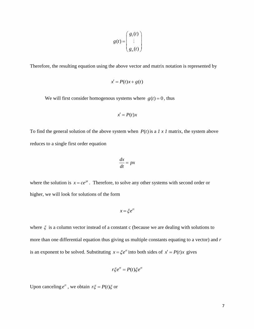
7
1( )
( )
( )n
g t
g t
g t
Therefore, the resulting equation using the above vector and matrix notation is represented by
( ) ( )x P t x g t
We will first consider homogenous systems where ( ) 0g t , thus
( )x P t x
To find the general solution of the above system when ( )P t is a 1 x 1 matrix, the system above
reduces to a single first order equation
dxpx
dt
where the solution is ptx ce . Therefore, to solve any other systems with second order or
higher, we will look for solutions of the form
rtx e
where is a column vector instead of a constant c (because we are dealing with solutions to
more than one differential equation thus giving us multiple constants equating to a vector) and r
is an exponent to be solved. Substituting rtx e into both sides of ( )x P t x gives
( )rt rtr e P t e
Upon canceling rte , we obtain ( )r P t or

8
( ( ) ) 0P t rI
where I is the n x n identity matrix. In order to solve ( ( ) ) 0P t rI , we will use theorem 1.
Theorem 1: Let A be an n x n matrix of constant real numbers and let X be an n-dimensional
column vector. The system of equations 0AX has nontrivial solutions, that is, 0X , if and
only if the determinant of A is zero.
In our case, ( ( ) )P t rI is the n x n matrix represented by A and is the n-dimensional column
vector represented by X. Therefore, in order to find the nontrivial solutions of ( ( ) ) 0P t rI ,
we must take the determinant of ( ( ) ) 0P t rI which is represented
11 1
1
( ) ( )
0
( ) ( )
n
n nn
p t r p t
p t p t r
Computing the determinant will yield a characteristic equation, which resembles the structure of
a polynomial of degree n, where the roots of the characteristic equation, eigenvalues denoted by
r, will be computed. After the eigenvalues have been computed, r will be substituted back into
( ( ) ) 0P t rI and solved for the nonzero vector, , which is called the eigenvector of the
matrix ( )P t corresponding to the eigenvalue 1r . The eigenvector will be an n x 1 column vector
that will have as many values as there are equations to solve for. After finding the eigenvalues
and the eigenvectors for those specific values, they will be substituted back into the equation
rtx e
which will be represented as the following specific solutions
9
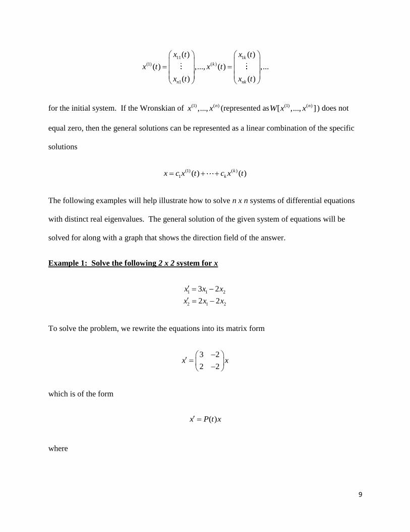
11 1
(1) ( )
1
( ) ( )
( ) ,..., ( ) ,...
( ) ( )
k
k
n nk
x t x t
x t x t
x t x t
for the initial system. If the Wronskian of (1) ( ),..., nx x (represented as (1) ( )[ ,..., ]nW x x ) does not
equal zero, then the general solutions can be represented as a linear combination of the specific
solutions
(1) ( )
1 ( ) ( )k
kx c x t c x t
The following examples will help illustrate how to solve n x n systems of differential equations
with distinct real eigenvalues. The general solution of the given system of equations will be
solved for along with a graph that shows the direction field of the answer.
Example 1: Solve the following 2 x 2 system for x
1 1 2
2 1 2
3 2
2 2
x x x
x x x
To solve the problem, we rewrite the equations into its matrix form
3 2
2 2x x
which is of the form
( )x P t x
where

10
3 2( )
2 2P t
We then find the eigenvalues of P(t) by finding the characteristic equation and solving for r.
Therefore,
23 2
det( ( ) ) 2 ( 1)( 2) 02 2
rP t rI r r r r
r
and the eigenvalues of P(t) are 1 1r and
2 2r . Now we compute the eigenvectors for each of
their respective eigenvalues. We will compute the nontrivial solutions of
1
2
3 20
2 2
cr
cr
For 1 1r
1 1 1 2
2 1
2 2 1 2
4 2 03 ( 1) 2 4 20 0 2
2 02 2 ( 1) 2 1
c c c cc c
c c c c
(Note that both of the resulting equations with 1c and
2c are the same). One such solution of the
equation is found by choosing 1 1c thus making
2 2c to give the eigenvector1
1
2
.
Knowing that ( ) ( )( ) nr tn nx t e , it follows that (1)
1
1( )
2
tx t c e
is a solution of the initial system.
For 2 2r
1 1 1 2
1 2
2 1 2
2 03 2 2 1 20 0 2
2 4 02 2 2 2 4n
c c c cc c
c c c c

11
By choosing 1 2c to solve the equation,
2 1c . Proper notation of eigenvectors, if possible,
insists that fractions should be avoided when representing the numerical value of the eigenvalue.
Therefore, for2 2r , 2
2
1
and a second solution is
(2) 2
2
2( )
1
tx t c e
Now, we check to see if we can represent 1x and
2x as a general solution by taking the Wronskian
of both specific solutions. The Wronskian of (1)( )x t and (2) ( )x t is
2
(1) (2)
2
2[ , ] 3
2
t t
t
t t
e eW x x e
e e
which is never equal to zero. It follows that the solutions (1)( )x t and (2) ( )x t are linearly
independent. Therefore, the general solution of the system ( )x P t x is
2
1 2
1 2( )
2 1
t tx t c e c e

12
All the general solutions (represented by the family of red lines), a combination of (1)( )x t and
(2) ( )x t , for which 1 0c and
2 0c , are asymptotic to the line 2 12x x . The blue trajectories
represent specific solutions to the system with each trajectory having a different initial value
(1 2(0) (0)x a and x b where a and b are any real number ).
For the remaining examples in this section, the derivation of the final solution will be
shown without all steps shown The purpose of these examples is to show the variety of systems
of differential equations that have distinct real eigenvalues such as a 3 x 3 system and a 2 x 2
system with initial conditions given.
Example 2: Solve the following 3 x 3 system for x
1 1 2 3
2 1 2 3
3 1 2 3
1 1 1
2 2 1 1
8 5 38 5 3
x x x x
x x x x x x
x x x x
First, we find the eigenvalues for the coefficient matrix by the following equation
1 1 1
det( ( ) ) 2 1 1 0
8 5 3
r
P t rI r
r
and solving the resulting characteristic equation.
>

13
>
Using maple yields the eigenvalues
1 2r , 2 2r , and
3 1r
and eigenvectors
1 2 3
4 0 3
5 , 1 , 4
7 1 2
The eigenvalues above are the same as the given Maple output but manipulated in properly
format where all values of the eigenvector are integers and the first value is positive. After the
eigenvalues and eigenvectors are computed, we find the Wronskian
(1) (2) (3)[ , , ] 12 0tW x x x e therefore we can substitute all the eigenvalues and eigenvectors
found into ( ) ( ) nr tn nx e and express the solution as a linear combination
(1) (2) (3) 2 2
1 2 3
4 0 3
( ) ( ) ( ) ( ) 5 1 4
7 1 2
t t tx t x t x t x t c e c e c e
Example 3: Solve the 2 x 2 system with initial conditions given for x
1 1 2 1
2 1 2 2
5 (0) 2 5 1 2 where where (0)
3 (0) 1 3 1 1
x x x xx x x
x x x x

14
We will start off the example by using Maple to find the eigenvalues and eigenvectors of the
coefficient matrix:
>
>
>
Therefore, 1 4r ,
11
1
, 2 2r , and
21
3
. The Wronskian (1) (2) 6[ , ] 2 0tW x x e
therefore the specific solutions (1)x and (2)x can be expressed as the general solution
4 2
1 2
1 1( )
1 3
t tx t c e c e
After the general solution has been found, we substitute 2
(0)1
x
into ( )x t to get
4*0 2*0
1 2 1 2
1 1 2 1 1 2(0)
1 3 1 1 3 1x c e c e c c
After the equation has been simplified, we multiply 1c and
2c by their respected vectors to yield
the follow system of equations
1 2 2c c and 1 23 1c c

15
We then solve the system of equations for 1c and
2c to get 1
7
2c and 2
3
2c
. Substituting
back into the general solution to get the specific solution of the system as
4 21 17 3
( )1 32 2
t tx t e e
The direction field of general solution along with a trajectory of the specific solution is
represented as
The above direction field shows the different families of solutions for the general solution
denoted by the red arrows and the blue trajectory represents the specific solution to the system
for when the initial starting value was 2
(0)1
x
. Now, after establishing the basis for solving
systems of differential equations, we will now delve into different cases of solving systems
where the eigenvalues are not real and/or distinct.

16
Section 2: Solving Systems of Differential Equations with Complex Eigenvalues
In this section, we will use what was previously discussed in the section for solving
systems with real and distinct eigenvalues on how to generate eigenvalues for an n x n system of
linear homogenous equations with constant coefficients denoted as
( )x P t x
Now if P(t) is real then the coefficients that make up the characteristic equation for r are real and
any complex eigenvalues must occur in conjugate pairs (Boyce & DiPrima, 2001, p. 384).
Therefore, for a 2 x 2 system, 1r a bi and
2r a bi would be eigenvalues where a and b are
real. Also, it follows that the corresponding eigenvectors are complex conjugate pairs of each
other. Therefore, 2 1r r and 2 1 . To help visualize this, take the equation that was formed
in the previous section
( ( ) ) 0P t rI
and substitute 1r and 1 into the equation to get
1
1( ( ) ) 0P t r I
which forms a corresponding general solution to the system. Now, by taking the complex
conjugate of the entire equation, the resulting equation becomes
1
1( ( ) ) 0P t r I
where P(t) and I are not affected by the conjugation because they both have all real values. The
equation then forms another corresponding general solution where 2 1r r and 2 1 . Now,

17
with the eigenvalues and eigenvectors solved for, we can use Euler’s formula to express a
solution with real and imaginary parts just as real solutions to the system. Euler’s formula states
cos sini te t i t
But, for use with general complex solutions to a system of differential equations, we will use the
a modified version of the formula
( ) (cos( ) sin( )) cos( ) sin( )i t t t te e t i t e t i e t
to find the real-value solutions to the system. We can choose either (1)( )x t or (2) ( )x t to find the 2
real-valued solutions because they are conjugates of each other and both will yield the same real-
valued solutions. Using (2) ( )x t and 2 a bi where a and b are real, then we have
(2) ( )( ) ( ) ( ) (cos( ) sin( ))i t tx t a bi e a bi e t i t
Factoring the above equation results in
(2) ( ) ( cos( ) cos( ) sin( ) sin( ))tx t e a t bi t ai t b t
and separating (2) ( )x t into its real and imaginary parts, (2) ( )x t will yield
(2) ( ) ( cos( ) sin( )) ( sin( ) cos( ))t tx t e a t b t ie a t b t
If (2) ( )x t is written as the sum of 2 vectors ( (2) ( ) ( ) ( )x t u t iv t ), then the vectors yielded are
( ) ( cos( ) sin( ))tu t e a t b t and ( ) ( sin( ) cos( ))tv t e a t b t

18
We can disregard the i in front of ( )v t because it is considered to be a multiplier of the vector
and we are only interested in the real-numbered vector solution. If we chose to solve for (1)( )x t
instead of (2) ( )x t , we would have gotten the same solution except (1)( ) ( ) ( )x t u t iv t . i is also
considered a multiplier of the ( )v t vector therefore we can disregard it and the answers for ( )u t
and ( )v t would be the same as the ones that were solved for above. ( )u t and ( )v t are the
resulting real-valued vector solutions to the system.
It is worth mentioning that ( )u t and ( )v t are linearly independent and can be expressed as
a single general solution. Therefore, for 1 2,r i r i and that
3,..., nr r are all real and
distinct. Let the corresponding eigenvectors be 1 2 3, , ,..., na bi a bi (Boyce &
DiPrima, 2001, p. 385). Then the general solution to systems of differential equations with
complex eigenvalues is
33
1 2 3( ) ( ) ( ) ... nr t r tn
nx t c u t c v t c e c e
where ( ) ( cos( ) sin( ))tu t e a t b t , ( ) ( sin( ) cos( ))tv t e a t b t , and P(t) consists of all
real coefficients. It is only when P(t) consists of all real coefficients that complex eigenvectors
and eigenvalues will occur in conjugate pairs (Boyce & DiPrima, 2001, p. 385). The following
examples will help illustrate how to solve n x n systems of differential equations with complex
eigenvalues. Both the complex and real-valued solutions will be given for each of the examples
and some direction fields will be shown to demonstrate the nature of systems with complex
eigenvalues.
19
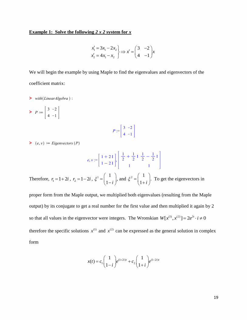
Example 1: Solve the following 2 x 2 system for x
1 1 2
2 1 2
3 2 3 2
4 4 1
x x xx x
x x x
We will begin the example by using Maple to find the eigenvalues and eigenvectors of the
coefficient matrix:
>
>
>
Therefore, 1 1 2r i ,
2 1 2r i , 1
1
1 i
, and
21
1 i
. To get the eigenvectors in
proper form from the Maple output, we multiplied both eigenvalues (resulting from the Maple
output) by its conjugate to get a real number for the first value and then multiplied it again by 2
so that all values in the eigenvector were integers. The Wronskian (1) (2) 2[ , ] 2 0tW x x e i
therefore the specific solutions (1)x and (2)x can be expressed as the general solution in complex
form
(1 2 ) (1 2 )
1 2
1 1( )
1 1
i t i tx t c e c ei i

20
But, we want to be able to find the real-valued solutions of the complex general solution so we
will use (1)x to find the real-valued vectors. Therefore,
(1) (1 2 )1
( )1
i tx t ei
Using Euler’s formula, (1)x becomes
1(cos(2 ) sin(2 ))
1
te t i ti
After Euler’s formula has been applied, we factor the above equation
cos(2 ) sin(2 )
cos(2 ) sin(2 ) cos(2 ) sin(2 )
tt i t
et i t i t t
and separate the real and imaginary elements into
cos(2 ) sin(2 )
sin(2 ) cos(2 ) sin(2 ) cos(2 )
t tt t
e iet t t t
The result is the two real-valued solutions of the form ( ) ( )u t iv t where
cos(2 ) sin(2 )( ) and ( )
sin(2 ) cos(2 ) sin(2 ) cos(2 )
t tt t
u t e v t et t t t
Therefore, the general solution to the system with real-valued solutions is
1 2 1 2
cos(2 ) sin(2 )( ) ( ) ( )
sin(2 ) cos(2 ) sin(2 ) cos(2 )
t tt t
x t c u t c v t c e c et t t t

21
The resulting direction field showing families of solutions to the general solution to the system is
The blue trajectories show specific solutions when initial conditions are given. Thus, the
direction field creates spiraled solutions where the origin is the center of the spirals called a
spiral point. The direction of the motion is away from the spiral point and the trajectories
become unbounded. Also, the spiral point, for this particular solution, is unstable. There are
also systems with complex eigenvalues where the general solution has a spiral point that is stable
because all trajectories approach it as t increases.
Example 2: Solve for the following 3 x 3 system for x
1 1
2 1 2 3
3 1 2 3
1 0 0
2 2 2 1 2
3 2 13 2
x x
x x x x x x
x x x x

22
Again, we will begin the example by using Maple to find the eigenvalues and eigenvectors of the
coefficient matrix:
>
>
>
Thus, the eigenvalues are1 1r ,
2 1 2r i , and 3 1 2r i . The simplified eigenvectors are
1
2
3
2
, 2
0
1
i
, and 3
0
1
i
. Notice that 1r and 1 already contain real-values therefore
no computations are needed to turn them into real-valued solutions like the other complex
eigenvalues and eigenvectors. The Wronskian (1) (2) (3) 3[ , , ] 4 0tW x x x e i therefore the
specific solutions (1)x , (2)x , (3)x and can be expressed as the general solution in complex form
(1 2 ) (1 2 )
1 2 3
2 0 0
( ) 3
2 1 1
t i t i tx t c e c i e c i e
To find the real-valued solutions of the general solution, we will use (2) ( )x t and Euler’s formula
in the following equations

23
(2) (1 2 )
0 0 0 0
( ) (cos(2 ) sin(2 )) cos(2 ) sin(2 )
1 1 sin(2 ) cos(2 )
i t t t tx t i e i e t i t e t ie t
t t
Therefore,
0 0
( ) cos(2 ) and ( ) sin(2 )
sin(2 ) cos(2 )
t tu t e t v t e t
t t
and the general solution to the system with real-valued solutions is
1
1 1 2 3 1 2 3
2 0 0
( ) ( ) ( ) 3 cos(2 ) sin(2 )
2 sin(2 ) cos(2 )
t t tx t c r c u t c v t c e c e t c e t
t t
Now that we know how to solve systems that yield real and/or imaginary eigenvalues and
eigenvectors, we will now focus our attention on the next case if a eigenvalue is repeated when
found from the characteristic equation.

24
Section 3: Solving Systems of Differential Equations with Repeated Eigenvalues
In this section, we will be solving systems of differential equations where the eigenvalues
found from the characteristic equation are repeated. We will still be finding solutions of the
following equation
( )x P t x
and will still find at least one of the eigenvalues/eigenvectors in the way we previously solved
systems with distinct eigenvalues. But, when solving for the other repeated eigenvalue, we will
see that the other solution will take the form
rt rtx te e
where and are constant vectors. After finding the first solution of the form (1) 1( ) rtx t e , it
may be intuitive to find a second solution to the system of the form
(2) 1( ) rtx t te
because of how repeated roots are solved when finding the solution to a second order differential
equation. Substituting that back into ( )x P t x yields
1 1 1 1 1 1 1( ) ( ) 0 1 ( ) 0rt rt rt rt rt rt rtr te e P t te r te e P t te e rt P t t
But, for the equation to be solved so it is satisfied for all t, the coefficients of rtte and rte must
each be zero (Boyce & DiPrima, 2001, p. 403). Therefore, we find out that in this case, 1 0
and thus 2 1 rtx te is not a solution for the second repeated eigenvalue. But, from

25
1 1 1( ) 0rt rt rtr te e P t te ,
we see that there is a form of rtx te in the substituted equation along with another term of the
form rte . Therefore, we need to assume that
2 1 rt rtx te e
Where and are constant vectors. Substituting the above expression into ( )x P t x gives
1 1 1 1 1 1( )( ) ( ) ( )( )rt rt rt rt rt rt rt rt rtr te e r e P t te e r te r e P t te e
Equating the coefficients of rtte and rte gives the following conditions
1 1 1 1 1( ) 0 ( ) 0 ( ( ) ) 0rt rtP t te r te P t r P t rI
1 1 1( ) 0 ( ) ( ( ) )rt rt rtP t e e r e P t r P t rI
for the determination of 1 and . The underlined portions are the important conditions derived
from the equation. To solve 1( ( ) ) 0P t rI , all we do is solve for one of the repeated
eigenvalue and eigenvector just like in previous sections. We will solve a matrix equation of the
form
1 1
11 1 1 1 11 1 1 1
1 1
1 1 1
( ) ( ) ( ) ( )
( ) ( ) ( ) ( )
n n n
n nn n n n nn n n
p t r p t p t r p t
p t p t r p t p t r
Solving for 1,..., n in the above equation will result in the solution of the vector denoted
26
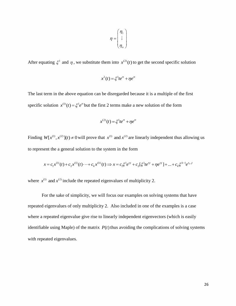
1
n
After equating 1 and , we substitute them into (2) ( )x t to get the second specific solution
2 1( ) rt rtx t te e
The last term in the above equation can be disregarded because it is a multiple of the first
specific solution (1) 1( ) rtx t e but the first 2 terms make a new solution of the form
(2) 1( ) rt rtx t te e
Finding (1) (2)[ , ]( ) 0W x x t will prove that (1) (2) and x x are linearly independent thus allowing us
to represent the a general solution to the system in the form
11 1 1(1) (1) ( ) 1 1 1
1 2 1 2( ) ( ) ( ) [ ] ... kr tr t r t r tk k
k kx c x t c x t c x t x c e c te e c e
where (1) (2) and x x include the repeated eigenvalues of multiplicity 2.
For the sake of simplicity, we will focus our examples on solving systems that have
repeated eigenvalues of only multiplicity 2. Also included in one of the examples is a case
where a repeated eigenvalue give rise to linearly independent eigenvectors (which is easily
identifiable using Maple) of the matrix ( )P t thus avoiding the complications of solving systems
with repeated eigenvalues.

27
Example 1: Solve the following 2 x 2 system for x
1 1 2
2 1 2
4 4 1
4 8 4 8
x x xx x
x x x
We will begin the example by using Maple to find the eigenvalues and eigenvectors of the
coefficient matrix:
>
>
>
Notice in the resulting eigenvectors that 2
0
0
which is a zero multiple of 1 and does us no
help in finding the second specific solution of the above system. But, the results derived from
Maple gives us 1 2 6r r ,
11
2
, and (1) 6
1( )
2
tx t e
. We need to use the equation
(2) 1( ) rt rtx t te e
to solve for and thus have a second specific solution to the system. To find out the second
specific solution, we substitute (2) 6 6
1( )
2
t tx t te e
into 4 1
4 8x x
to get the following
expression

28
1 16 6 6 6 6
2 2
1 1 4 1 1 4 16 6
2 2 4 8 2 4 8
t t t t te te e te e
Multiplying out 64 1 1
4 8 2
tte
and factoring out a 6 from the result yields
1 16 6 6 6 6
2 2
1 1 1 4 16 6 6
2 2 2 4 8
t t t t te te e te e
Canceling out the 6
16
2
tte
on each side of the equation and rearranging the equation yields
1 16 6 6
2 2
4 1 16
4 8 2
t t te e e
Factoring out 1 6
2
te
on the left side of the equation and simplifying gives us
1 6 6
2
1 6 6
2
1
2
4 1 16
4 8 2
4 1 6 0 1
4 8 0 6 2
2 1 1
4 2 2
t t
t t
I e e
e e
The end product of the above expression,1
2
2 1 1
4 2 2
, is of the form 1( ( ) )P t rI .
In this case

29
14 1 6 0 1
( ( ) )4 8 0 6 2
P t rI
Thus, to solve for , we solve
1 1 2
1 2
2 1 2
2 12 1 1 00 and 1
4 2 24 2 2 1
(Note that both of the resulting equations with 1 and
2 are the same). After solving for , we
substitute it into (2) 1( ) rt rtx t te e to find the second solution of the system to be
(2)1 0
( )2 1
rt rtx t te e
The Wronskian (1) (2) 12[ , ] 0tW x x e . Therefore the specific solutions (1)x and (2)x can be
expressed as the general solution
6 6
1 2
1 1 0( )
2 2 1
t tx t c e c t e
The resulting direction field showing families of solutions to the general solution to the system is

30
The blue trajectories show specific solutions when initial conditions are given. The origin is
called an improper node. If the eigenvalues are negative, then the trajectories are similar but
traversed in the inward direction. An improper node is asymptotically stable or unstable,
depending on whether the eigenvalues are negative or positive (Boyce & DiPrima, 2001, p. 404).
Example 2: Solve the following 3 x 3 system for x
1 1 2 3
2 2 3
3 3
2 1 2 1
0 1 1
0 0 22
x x x x
x x x x x
x x
We will begin the example by using Maple to find the eigenvalues and eigenvectors of the
coefficient matrix:
>

31
>
>
From the Maple results: 1 2 1r r ,
3 2r , 1
1
( ) 0
0
tx t e
, and 3 2
1
( ) 1
1
tx t e
. What we need to
find is the specific solution to (2) ( )x t . In this example, we will use the equation 1( ( ) )P t rI
to solve for , substitute it into (2) 1( ) rt rtx t te e , and use the shortcut to find out the third
specific solution to the system. Therefore
1
1
2
3
1
2
3
1 2 1 1
( ( ) ) 0 1 1 1 0
0 0 2 0
0 2 1 1
0 0 1 0
0 0 1 0
t t
t t
P t rI I e e
e e
and
2 3
3 1 2 3
3
02 1
1 10 0, , 0
2 20
0

32
Substituting what we found for into (2) 1( ) rt rtx t te e yields
(2)
01 2 0
1( ) 0 0 1
20 0 0
0
t t t tx t te e te e
The Wronskian (1) (2) (3) 4[ , , ] 0tW x x x e . Therefore, the specific solutions (1) (2) (3), ,x x and x can
be expressed as the general solution
2
1 2 3
1 1 2 0
( ) 1 0 0 1
1 0 0 0
t t tx t c e c e c t e
Example 3: Solve the following 3 x 3 system for x
1 2 3
2 1 2 3
3 1 2 3
3 0 1 3
2 3 3 2 3 3
2 1 12
x x x
x x x x x x
x x x x
For this example, using Maple can unlock a potential shortcut in solving for the general solution
to the above system. Again, we will begin the example by using Maple to find the eigenvalues
and eigenvectors of the coefficient matrix:
>
>

33
>
Unlike the other 2 examples, the Maple output displays 2 linearly independent eigenvectors of
the repeated eigenvalues2 3 2r r . Another shortcut for finding eigenvectors of repeating
eigenvalues is found if a math program, such as Maple, is utilized to solve systems of differential
equations. Therefore
1 2 2 2 3 2
1 1 3
( ) 1 , ( ) 2 , ( ) 0
1 0 2
t t tx t e x t e x t e
and the general solution to the system is
2 2
1 2 3
1 1 3
1 2 0
1 0 2
t tx c e c c e
A more advanced look at systems with repeated eigenvalues would include repeated
eigenvalues with multiplicities higher than 2. The equations to solve higher multiplicities of
repeated eigenvalues become more detailed and difficult to solve for but to find the eigenvalues
for such values, we would follow the same thought process in how we found the eigenvalue for
repeated eigenvalues of multiplicity 2. For the next section, we will return to our original form

34
of a differential equation 1 1( ) ... ( ) ( )n nx p t x p t x g t and solve nonhomogenous systems
where the value of ( ) 0g t .

35
Section 4: Solving Systems of Nonhomogenous Differential Equations
Unlike the previous sections where we solved different types of systems of homogeneous
differential equations with constant coefficients, this section will focus on solving systems of
nonhomogenous differential equations of the form
( ) ( )x P t x g t
The following theorem related to nonhomogenous systems should help us figure out
where to start solution process:
Theorem 2: If (1) ( )( ),..., ( )nx t x t are linearly independent solutions of the n-dimensional
homogenous system ( )x P t x on the interval a < t < b and if ( )px t is any solution of the
nonhomogenous system ( ) ( )x P t x g t on the interval a < t < b, then any solution of
the nonhomogenous system can be written (1) ( )
1 ( ) ( ) ( )n
k px c x t c x t x t for a unique
choice of the constants1,..., nc c (Rainville, Bedient, & Bedient, 1997, p. 199).
The theorem states that we will need to find a particular solution ( )px t and add it on to the
general solution of the homogenous system that is part of the nonhomogenous system. To do
that, we will be using a variation of parameters technique to find ( )px t and solve the equation
( ) ( )x P t x g t .
Solutions of the homogenous part of the nonhomogenous systems will take the form
11
1nr tr t n
nx c e c e
and using the variation of parameters technique suggests we seek a solution to the
nonhomogenous system to be

36
11
1( ) ( ) ( ) nr tr t n
p nx t c t e c t e
Direct substitution back into ( ) ( )x P t x g t yields
1 1 11 1 1
1 1 1 1( ( ) ( ) ) ( ( ) ( ) ) ( ( ) ( ) ( ) ( ) ) ( )n n nr t r t r tr t r t r tn n n
n n n nrc t e r c t e c t e c t e P t c t e P t c t e g t
( )P t multiplied by any eigenvalue found to be a part of the specific solution will result in that
particular eigenvalue multiplied by its eigenvector because it is already part of the solution to the
homogeneous system. Therefore
1 1 1
1
1 1 1
1 1 1 1 1
1
1
( ( ) ( ) ) ( ( ) ( ) ) ( ( ) ( ) ) ( )
( ( ) ( ) ) ( )
n n n
n
r t r t r tr t r t r tn n n
n n n n n
r tr t n
n
rc t e r c t e c t e c t e rc t e r c t e g t
c t e c t e g t
The resulting equation can be rewritten in matrix form as
11
1 1 1 1
1
( ) ( )
( ) ( )n
r tn
r tn
n n n n
c t e g t
c t e g t
To solve for 1( ),..., ( )nc t c t , we must use Cramer’s Rule to solve Ax b for x where
11
1 1 1 1
1
( ) ( )
, ,
( ) ( )n
r tn
r tn
n n n n
c t e g t
A x b
c t e g t
Cramer’s Rule states that the system has a unique solution that is given by
det( )1,...,
det( )
kk
Bx for k n
A

37
Therefore
1
1
1 1 1 1
1
1 1 1
1 1 1 1
1 1
( ) ( )
( ) ( )( ) ,..., ( ) n
n
n
n n n nr tr t
nn n
n n
n n n n
g t g t
g t g tc t e c t e
Thus,
1 1
1 1 1 1 1 1
1 1 1 1
( ) ( ) ... ( ) ( ) [ ( ) ... ( )]
( ) ( ) ... ( ) ( ) [ ( ) ... ( )]n n
r t r t
n n n n
r t r t
n n n n n n
c t e a g t a g t c t a g t a g t e
c t e b g t b g t c t b g t b g t e
for some arbitrary constants 1 1,..., and ,...,n na a b b . To solve for the general solution, integrate
both sides of the above equation to get 1( ),..., ( )nc t c t , substitute them into
11
1( ) ( ) ( ) nr tr t n
p nx t c t e c t e to find the particular solution, and substitute ( )px t into
(1) ( )
1 ( ) ( ) ( )n
k px c x t c x t x t to find the general solution for the system. The following
examples will help demonstrate how to solve systems of nonhomogenous differential equations
and lead into an application of nonhomogenous systems.
Example 1: Solve the following 2 x 2 system for x
1 2
2 1 2
0 1 0
2 3 32 3 3tt
x xx x
ex x x e
We will begin the example by using Maple to find the eigenvalues and eigenvectors of the
homogenous part of the system

38
0 1
2 3x x
Therefore
>
>
>
The resulting eigenvalues and eigenvectors are 1 2
1 2
1 11, 2, , and
1 2r r
. The
Wronskian (1) (2) 12[ , ] 0tW x x e thus, the general solution to the homogenous part of the system
is
2
1 2
1 1
1 2
t t
hx c e c e
To find the particular solution of the nonhomogenous part of the system, we will use the
variation of parameters technique to find a solution of the above equation of the form
2
1 2
1 1( ) ( )
1 2
t t
px c t e c t e
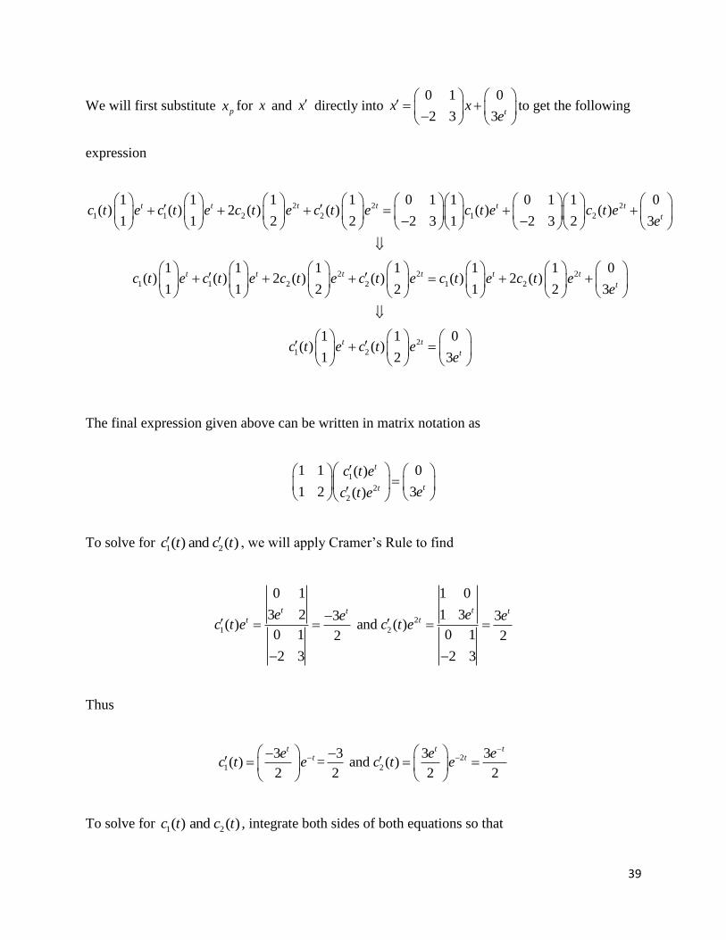
39
We will first substitute px for x and x directly into
0 1 0
2 3 3 tx x
e
to get the following
expression
2 2 2
1 1 2 2 1 2
2
1 1 2 2
1 1 1 1 0 1 1 0 1 1 0( ) ( ) 2 ( ) ( ) ( ) ( )
1 1 2 2 2 3 1 2 3 2 3
1 1 1 1( ) ( ) 2 ( ) ( )
1 1 2 2
t t t t t t
t
t t t
c t e c t e c t e c t e c t e c t ee
c t e c t e c t e c t
2 2
1 2
2
1 2
1 1 0( ) 2 ( )
1 2 3
1 1 0( ) ( )
1 2 3
t t t
t
t t
t
e c t e c t ee
c t e c t ee
The final expression given above can be written in matrix notation as
1
2
2
1 1 0( )
1 2 3( )
t
tt
c t e
ec t e
To solve for 1 2( ) and ( )c t c t , we will apply Cramer’s Rule to find
2
1 2
0 1 1 0
3 2 1 33 3( ) and ( )
0 1 0 12 2
2 3 2 3
t tt tt te ee e
c t e c t e
Thus
2
1 2
3 3 3 3( ) = and ( )
2 2 2 2
t t tt te e e
c t e c t e
To solve for 1 2( ) and ( )c t c t , integrate both sides of both equations so that

40
1 2
3 3( ) and ( )
2 2
tt ec t c t
and substituting into the partial solution 2
1 2
1 1( ) ( )
1 2
t t
px c t e c t e
yields
21 1 1 13 3
3 31 2 1 22 2
tt t t t
p
t ex e e te e
Therefore, the general solution to the nonhomogenous system is
2
1 2
1 1 1 13 3
1 2 1 2
t t t t
h px x x c e c e te e
Example 2: Solve the following 2 x 2 system for x
1 1 2
2 1 2
2 12
1 22 3 3
t tx x x e ex x
x x x t t
We will begin the example by using Maple to find the eigenvalues and eigenvectors of the
homogenous part of the system
2 1
1 2x x
Therefore
>
>

41
>
The resulting eigenvalues and eigenvectors are 1 2
1 2
1 11, 3, , and
1 1r r
. The
Wronskian (1) (2) 12[ , ] 0tW x x e thus, the general solution to the homogenous part of the system
is
3
1 2
1 1
1 1
t t
hx c e c e
To find the particular solution of the nonhomogenous part of the system, we will use the
variation of parameters technique to find a solution of the above equation of the form
3
1 2
1 1( ) ( )
1 1
t t
px c t e c t e
Substituting px for x and x directly into
2 1
1 2 3
tex x
t
to get the following
3
1 2
1 1( ) ( )
1 1 3
t
t t ec t e c t e
t
The final expression above can be written in matrix notation as
1
3
2
1 1 ( )
1 1 ( ) 3
t t
t
c t e e
c t e t
To solve for 1 2( ) and ( )c t c t , we will apply Cramer’s Rule to find

42
3
1 2
3 3( ) and ( )
2 2 2 2
t tt te t e t
c t e c t e
Thus
2 3
1 2
1 3 3( ) and ( )
2 2 2 2
t t tte e tec t c t
To solve for 1 2( ) and ( )c t c t , integrate both sides of both equations so that
2
1 2
2 23
1 2
3 3 3 3( ) + and ( )
2 2 2 4 2 2
1 1 1 13 3 3 3( ) ( ) +
1 1 1 12 2 2 4 2 2
tt t t t
t t t tt t
h p
ete e t te ec t c t
t te e te ex x x c t e c t e
and substituting into the partial solution 3
1 2
1 1( ) ( )
1 1
t t
px c t e c t e
yields
2
3
2 2
1 13 3 3 3+
1 12 2 2 4 2 2
1 13 3 3 3+
1 12 2 2 4 2 2
tt t t tt t
p
t t t t
p
ete e t te ex e e
t te e te ex
Therefore, the general solution to the nonhomogenous system is
2 23
1 2
1 1 1 13 3 3 3( ) ( ) +
1 1 1 12 2 2 4 2 2
t t t tt t
h p
t te e te ex x x c t e c t e

43
Section 5: Application of Systems of Differential Equations – Arms Races
(Nonhomogenous Systems of Equations)
In the previous section, we discussed how to solve systems of differential equations that
were nonhomogenous using a variation of parameters technique. Now, we can apply that
knowledge of solving systems with nonhomogenous equations to solve a model that illustrates an
arms race between two competing nations. L.F. Richardson, an English meteorologist, first
proposed this model (also known as the Richardson Model) that tried to mathematically explain
an arms race between two rival nations. Richardson himself seemed to have believed that his
perceptions relating to the way nations compete militarily might have been useful in preventing
the outbreak of hostilities in World War II (Brown, 2007, p. 60). Both nations are self-defensive,
both fight back to protect their nation, both maintain army and stock weapons, and when one
nation expands their army the other nation finds it offensive. Therefore, both nations will spend
money (in billions of dollars) on armaments x and y that are functions of time t measured in
years. x(t) and y(t) will represent the yearly rate of armament expenditures of the two nations
using some standard unit. Richardson then made some of the following assumptions about his
model:
The expenditure for armaments of each country will increase at a rate that is proportional
to the other country’s expenditure (each nation's mutual fear's rate is directly proportional
to the expenditure of the other nation) (Rainville, Bedient, & Bedient, 1997, p. 228).
The expenditure for armaments of each country will decrease at a rate that is proportional
to its own expenditure (extensive armament expenditures create a drag on the nation's
economy) (Rainville, Bedient, & Bedient, 1997, p. 228).

44
The rate of change of arms expenditure for a country has a constant component that
measures that level of antagonism of that country toward the other (Rainville, Bedient, &
Bedient, 1997, p. 228).
The effects of the three previous assumptions are additive (Rainville, Bedient, & Bedient,
1997, p. 228).
The previous assumptions make up the differential equations of the arms race system denoted by
0
0
(0)
for
(0)
dx x xay mx rdt
dybx ny s y y
dt
where a, m, b, and n are all positive constants. The positive terms ay and bx represent the drive to
spend more money are arms due to the level of spending of the other nation, and the negative
terms mx and ny reflect a nation’s desire to inhibit future military spending because of the
economic burden of its own spending. But, r and s can be any value because they represent the
attitudes of each nation towards each other (negative values represent feelings of good will while
positive values represent feelings of distrust). The initial values (0) and (0)x y represent the
initial amount of money (in billions of dollars) each nation will spend towards armaments. The
system can be simplified into
( )
( )
x t mx ay r
y t bx ny s
and is expressed in matrix notation where
( ) ( )( )
( ) ( )
x t m a x t rX P t X B
y t b n y t s

45
To solve for the system, we will use the knowledge from the previous section to develop
general solutions to the homogenous system. For the nonhomogenous part of the system, the
solution will be a constant solution of the form f
g
because the vector B is made up of
constants thus making the process of solving by variation of parameters much easier. Lastly, the
initial values (trajectories) for the solution will represent the starting amount of money each
country will be spending on armaments.
General solutions to the arms race system will represent one of a few types of races: a
stable arms race, a runaway arms race, a disarmament, or disarmament/runaway/stable arms race
depending on the initial values. The following examples will help demonstrate each of the above
mentioned arms races along with slope fields to graphically represent the races.
Example 1: A Runaway Arms Race
The following system will result in a runaway arms race:
( ) 2 4 8 2 4 8
( ) 4 2 2 4 2 2
x t x yX X
y t x y
To find the solution to this arms race, we will first find the general solution to the
homogenous part of the system using Maple:
>
>
>

46
Therefore, 1 2r , 1
1
1
, 2 6r , and 2
1
1
. The Wronskian (1) (2) 4[ , ] 2 0tW x x e
thus, the general solution to the homogenous part of the arms race is
2 6
1 2
1 1
1 1
t t
hx c e c e
As mentioned in the beginning of this section, the nonhomogenous system
( )X P t X B has a constant solution of the form e
f
because B is a vector of constants thus
the solution should also be a vector made up of constants. Therefore, in the equation
( )X P t X B , ( )e
X tf
can be substituted into and X X where
2 4 8( ) and
4 2 2P t B
to get the following expression
2 4 8 2 4 8 2 4 8 20
4 2 2 4 2 2 4 2 2 3n
f f f g fx
g g f g g
Therefore the general solution of the nonhomogenous system is
2 6
1 2
1 1 2
1 1 3
t t
h nx x x c e c e
47
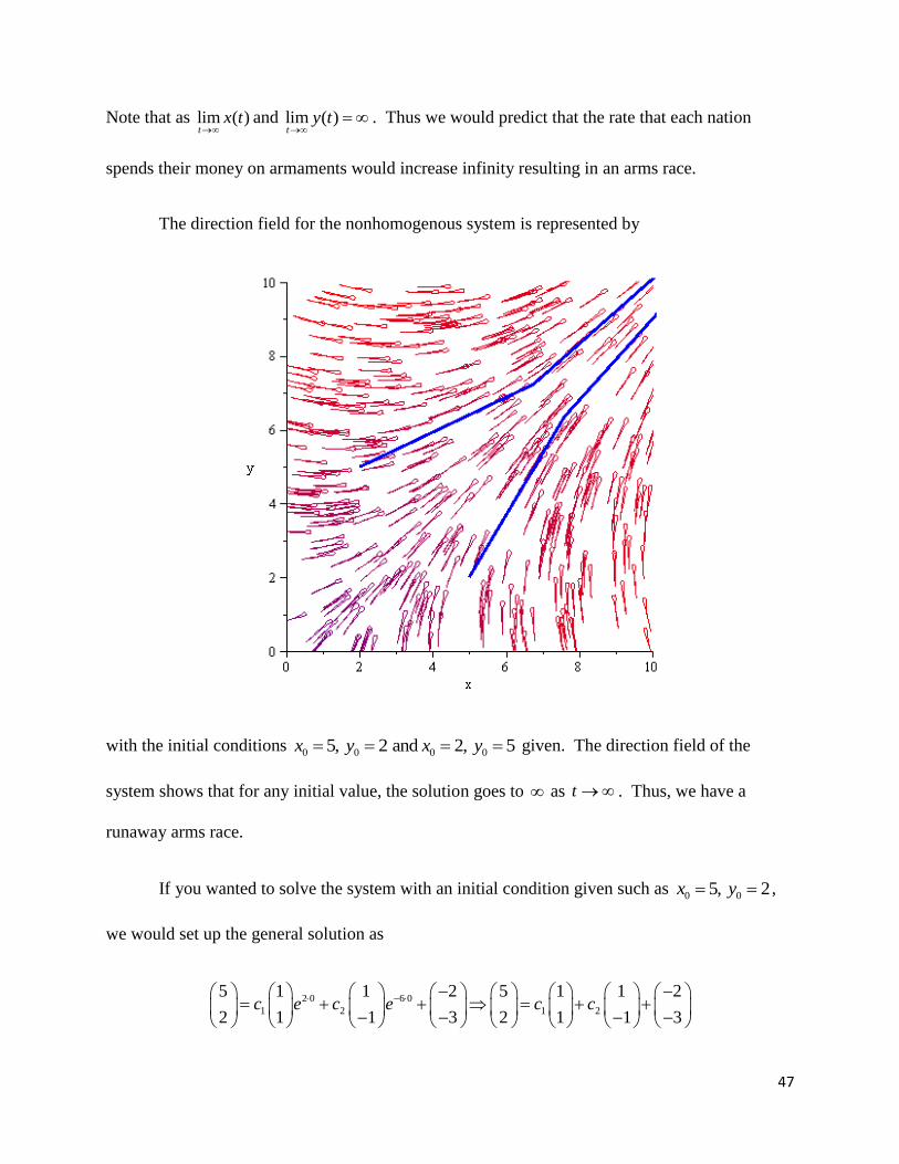
Note that as lim ( )t
x t
and lim ( )t
y t
. Thus we would predict that the rate that each nation
spends their money on armaments would increase infinity resulting in an arms race.
The direction field for the nonhomogenous system is represented by
with the initial conditions 0 0 0 05, 2 and 2, 5x y x y given. The direction field of the
system shows that for any initial value, the solution goes to as t . Thus, we have a
runaway arms race.
If you wanted to solve the system with an initial condition given such as 0 05, 2x y ,
we would set up the general solution as
2 0 6 0
1 2 1 2
5 1 1 2 5 1 1 2
2 1 1 3 2 1 1 3c e c e c c

48
and solve for 1c and
2c . Therefore
1 2 1 2
1 2 1 2
1 2 1 2
2 5 75 1 1 26 and 1
3 2 62 1 1 3
c c c cc c c c
c c c c
Thus, the final solution with the initial conditions given is
2 61 1 2
61 1 3
t tx e e
or
2 6
2 6
( ) 6 2
( ) 6 3
t t
t t
x t e e
y t e e
The role of the initial value is how much each nation will initially spend on armaments in
billions of dollars. Using initial values when solving an arms race system will lead to a specific
solution describing the race instead of families of general solutions describing all cases of the
system.
Example 2: A Stable Arms Race
The following system will result in a stable arms race:
( ) 5 2 1 5 2 1
( ) 4 3 2 4 3 2
x t x yX X
y t x y
To find the solution to this arms race, we will first find the general solution to the
homogenous part of the system using Maple:

49
>
>
>
Therefore, 1 7r , 1
1
1
,
2 1r , and 21
2
. The Wronskian (1) (2) 8[ , ] 3 0tW x x e
thus, the general solution to the homogenous part of the arms race is
7
1 2
1 1
1 2
t tx c e c e
The general solution to the nonhomogenous part of the arms race will be found by
substituting ( )f
X tg
into 5 2 1
4 3 2X X
. Therefore
5 2 1 5 2 1 00 1 and 2
4 3 2 4 3 2 0
f f gf g
g f g
and the solution of that system is 1
2nx
. Thus the general solution of the nonhomogenous
system is
7
1 2
1 1 1
1 2 2
t t
h nx x x c e c e

50
Note that as lim ( ) 1t
x t
and lim ( ) 2t
y t
because in both equations, the terms with both
7 and t te e go to 0 as t . All that is left from the differential equations are the constant
terms ( ) 1 and ( ) 2x t y t and what initial values of the system converge to.
The direction field with a few trajectories denoting the initial values for the
nonhomogenous system is represented by
The direction field of the system shows that for any initial value, the solution approaches the
point (1,2) as t . Thus, we have a stable arms race.

51
Example 3: Disarmament
The following system
( ) 4 1 4 1 1
( ) 2 1 1 2
x t x yX X
y t x y
will result in disarmament between the competing nations for all initial values.
For the sake of simplicity, only the graph of this system and the solution solved by Maple
will be shown because the eigenvectors and eigenvalues generated from P(t) become
complicated radicals that would be difficult to manipulate by hand to find an answer. Therefore,
the general solution to the system given by Maple output is
>
>
>
>

52
>
As you can see from the above solution, the general solution to the system is becomes very
complicated but, lim ( ) 1 and lim ( ) 3t t
x t y t
thus showing that eventually, the nations will
get to a point in time where they are decreasing the rate at which they are spending money on
armaments until they are spending no money on the arms race. The graph of the system is much
more beneficial in demonstrating an arms race that ends in disarmament.
The direction field with a few trajectories denoting the initial values for the
nonhomogenous system is represented by

53
For the initial values represented by the blue trajectories in the above directional field, the
trajectories will approach the point ( 1, 3) as t thus resulting in disarmament with any
initial value chosen for the system.
Example 4: Disarmament/Runaway Arms Race/Stable Arms Race
The following system
( ) 2 4 2 2 4 2
( ) 4 2 2 4 2 2
x t x yX X
y t x y
will result in disarmament if 0 0 2x y , a runaway arms race if
0 0 2x y , or a stable arms
race if 0 0 2x y .
To find the solution to this arms race, we will first find the general solution to the
homogenous part of the system using Maple:
>
>
>
Therefore, 1 2r ,
11
1
, 2 6r , and
21
1
. The Wronskian (1) (2) 4[ , ] 2 0tW x x e
thus, the general solution to the homogenous part of the arms race is

54
2 6
1 2
1 1
1 1
t t
hx c e c e
The general solution to the nonhomogenous part of the arms race will be found by
substituting ( )f
X tg
into 2 4 2
4 2 2X X
. Therefore
2 4 20 1 and 1
4 2 2
ff g
g
and the solution of the system is 1
1nx
. Thus the general solution of the nonhomogenous
system is
2 6
1 2
1 1 1
1 1 1
t t
h nx x x c e c e
The direction field with a few trajectories denoting the initial values for the nonhomogenous
system is represented by

55
For the initial values 0 0 0 0 0 01.7, 0, 0, 1.7, and 2x y x y x y in the above directional
field, the trajectories will approach as t thus resulting in disarmament. For the initial
values0 0 0 0 0 02, 0, 0, 2, and 2x y x y x y , the trajectories will approach the point (1,1)
as t thus resulting in a stable arms race. For the initial values
0 0 0 0 0 03, 0, 0, 3, and 2x y x y x y , the trajectories will go to as t thus resulting
in a runaway arms race.
Conjectures of Richardson’s Arms Race Model
After solving and graphing results of the Arms Race Model to show the different situations in
describing the model, in the following conjectures can be made to better summarize what is
theoretically happening in the model with certain values for the coefficients:
If mn - ab < 0, r > 0, and s >0, there will be a runaway arms race.
If mn - ab> 0, r > 0, and s > 0, there will be a stable arms race.
If mn - ab > 0, r < 0, and s < 0, there will be disarmament.
If mn - ab < 0, r < 0, and s < 0, there will be disarmament if 0 02
r sx y
, a runaway
arms race if 0 02
r sx y
, and a stable arms race if 0 0
2
r sx y
.
Real World Examples of Richardson’s Model
At the level of strategic weapons during the Cold War, Russia and America were
in a two-way arms race. The structure of this is that both sides increased until the
Russians achieved equality, at which point the two sides began signing initial SALT
agreements as predicted by the model (Hunter, 1980, p. 252).

56
Both nations realized that once they were at equality, that the risk of spending more money on
armaments would have worse impact on their economies thus, as the model predicted, the arms
race started to stabilize (even though both nations still have negative feelings toward each other).
Another example reveals sharp limitation on the model. In 1939, Russia and Germany
signed a nonaggression pact which left Germany and Russia in a two-sided alliance
against England, France, and other weaker countries. Yet the arms race in both Russia
and Germany accelerated at the maximum economic rate. Why? Because both sides knew
that Hitler intended to invade Russia at the earliest feasible time (Hunter, 1980, p. 252).
Both nations secretly had negative feelings towards one another and were willing to spend more
money on armaments without much regard on the negative impact that the spending would have
on their economy. Thus, as Richardson’s Model could have predicted, the Germans and the
Russians were at a runaway arms race with each other (at the time).
Richardson’s Arms Race Model Extended
What was described in this section was the most generic model of the arms race. The
model has been expanded to include more than two nations and other variables that would affect
an arms race. What was interesting is that the arms race model could and was used to model
World War II which included numbers for 10 countries that were included. At the most basic
level of the arms race model, a lot of problems and difficulties arrive that are solved in more
detailed versions of the model but, Richardson’s Model laid a good foundation to understand a
social science topic mathematically.

57
Section 6: Application of Systems of Differential Equations – Predator-Prey Model
(Nonlinear System of Equations)
In the study of the dynamics of a single population, ecologists typically take into
consideration such factors as the "natural" growth rate and the "carrying capacity" of the
environment. Mathematical ecology requires the study of populations that interact, thereby
affecting each other's growth rates. In this section we study a very special case of such an
interaction, in which there are exactly two species, one of which, the predators, eats the other, the
prey. Such pairs exist throughout nature: Lions and gazelles, birds and insects, pandas and
eucalyptus trees, and Venus fly traps and flies (Moore & Smith, 2003).
Vito Volterra (1860-1940) was a famous Italian mathematician who retired from a
distinguished career in pure mathematics in the early 1920s. His son-in-law, Humberto
D'Ancona, was a biologist who studied the populations of various species of fish in the Adriatic
Sea. In 1926, D'Ancona completed a statistical study of the numbers of each species sold on the
fish markets of three ports from 1914-1923: Fiume, Trieste, and Venice (Moore & Smith, 2003).
D'Ancona observed that the highest percentages of predators occurred during and just
after World War I, when fishing was drastically curtailed. He concluded that the
predator-prey balance was at its natural state during the war and that intense fishing
before and after the war disturbed this natural balance. Having no biological or
ecological explanation for this phenomenon, D'Ancona asked Volterra if he could come
up with a mathematical model that might explain what was going on. In a matter of
months, Volterra developed a series of models for interactions of two or more species
58
(Moore & Smith, 2003). The first and simplest of these models is the subject of this
section.
Alfred J. Lotka (1880-1949) was an American mathematical biologist who formulated
many of the same models as Volterra, independently and at about the same time. His primary
example of a predator-prey system comprised a plant population and an herbivorous animal
dependent on that plant for food (Moore & Smith, 2003). Thus, the Predator-Prey Model is also
known as Lotka-Volterra Model named after the two mathematicians that helped developed the
equations.
To keep the model simple for easier understanding, we will make the following
assumptions that would be unrealistic in most predator-prey interactions:
The predator species is totally dependent on a single prey species as its only food supply.
The prey species has an unlimited food supply.
There is no threat to the prey other than the specific predator.
In constructing the model between the two species, we will make the following
assumptions to set up the model which relate to the above assumptions:
( )x t will represent the number of prey at a time given by t and ( )y t will represent the
number of predators at a time also given by t.
In the absence of the predator, the prey grows at a rate proportional to the current
population; thus , 0, when 0dx
ax a ydt
(Boyce & DiPrima, 2001, p. 503).

59
In the absence of the prey, the predator dies out; thus , c 0, when 0dy
cy xdt
(Boyce
& DiPrima, 2001, p. 503).
The number of encounters between predator and prey is proportional to the product of
their populations. Each such encounter tends to promote the growth of the predator and
to inhibit the growth of the prey. Thus the growth rate of the predator is increased by a
term of the form pxy , while the growth rate of the prey is decreased by a term bxy ,
where p and b are positive constants (Boyce & DiPrima, 2001, p. 503).
As a result of these assumptions, the following equations were formulated to represent the
change of predators and prey over time
( ) and ( )dx dy
ax bxy x a by cy pxy y c pxdt dt
where a, c, b, and p are all positive. The growth rate of the prey and the death rate of the
predator is represented by a and c respectively while b and p are measures of the effect of the
interaction between the two species (Boyce & DiPrima, 2001, p. 504). Even though the
differential equations of the Predator-Prey Model are nonlinear, we can use the linear part of the
equation to find a general solution to help explain the behavior of the system. Also, finding the
critical points, the directional field, and trajectories of the directional field will be key in further
explaining the behavior of the system. The critical points of the system are the solutions of
( ) 0 and ( ) 0x a by y c px
that is the points (0,0) and ( / , / )c p a b . We first examine the solutions of the corresponding
linear system near each critical point. The origin is a saddle point and hence unstable. Entrance

60
to the saddle point is along the y-axis and departs via the x-axis. All other trajectories depart
from the neighborhood of the critical point.
From the critical point at the origin, the corresponding linear system is
0(1)
0
x a xd
y c ydt
The eigenvalues and eigenvectors are
1 1
1 2
1 0, , , and
0 1r a r c
Therefore, the general solution is
1 2
1 0
0 1
at ctx
c e c ey
and the resulting direction field is

61
Next, consider the critical point ( / , / )c p a b . To examine the behavior and generate a general
solution around that critical point, we will add values u and v to them to get
and c a
x u y vp b
. Then we will substitute them into ( ) 0 and ( ) 0x a by y c px to
translate and c a
u x v yp b
. Therefore
0 and 0
0 and 0
0 and 0
c a a cu a b v v c p u
p b b p
c au a a bv v c c pu
p b
bc apv bu u pv
p b
Therefore, the corresponding linear system is
0(2)
0
u bc p ud
v ap b vdt
The eigenvalues of that system are r i ac so the critical point (stable) is along the y-axis;
all other trajectories depart from the neighborhood of the critical point (Boyce & DiPrima, 2001,
p. 507).

62
Returning to the nonlinear system, it can be reduced to a single equation represented as
( )
( )
dy dy dt y c px
dx dx dt x a by
The above equation can be separated and integrated to get the following solution
ln ln (3)a y by c x px C
where C is a constant of integration.

63
Even though we cannot solve the solution for x or y, the solution does show that the graph
of the equation for a fixed value of c is a closed curve surrounding the nonzero critical
point. Thus the critical point is also a center of the initial nonlinear system and the
predator/prey populations exhibit a cyclic variation (Boyce & DiPrima, 2001, p. 506).
The following examples will help demonstrate the Predator-Prey Model and the aspects
mentioned above that it contains.
Example 1: Determine the Behavior of x and y as t→∞
(1.5 0.5 ) and ( 0.5 )dx dy
x y y xdt dt
First, we will find the critical points of the system by using ( ) 0 and ( ) 0x a by y c px to
find the points
(0,0) and (1 2,3)
Next, we will examine the behavior at the critical point (0,0) by using equation (1)
0 1.5 0
0 0 0.5
x a x x xd d
y c y y ydt dt
Therefore, the eigenvalues and eigenvectors of the above equation are
1 1
1 2
1 01.5, , 0.5, and
0 1r r
and its general solution is

64
1.5 0.5
1 2
1 0
0 1
t tx
c e c ey
After examining the first critical point, we will examine the second critical point (1 2,3) by using
equation (2)
0 0.5 0.5 10
1.5 1 0.5 00
0 0.25
3 0
u bc p u u ud d
v ap b v v vdt dt
u ud
v vdt
The resulting eigenvalues are 1 2
3 3 and
2 2
i ir r . The resulting eigenvalues have
radicals and complex values that are difficult to express in simpler terms.
The original system has a solution from equation (3)
ln ln 1.5ln 0.5 0.5lna y by c x px C y y x x C

65
The resulting directional field with trajectories for different initial populations of the
predator and prey is
The directional field and trajectories show the populations of predator and prey over time. The
ellipses around the critical point (1 2,3) show that over a certain period of time, the way in how
the predator and prey interact with each other go through a cycle of change and end up back at
the initial population of both the predator and the prey. Because the predator/prey start from a
relatively small population, the prey increase first because there is little predation. Then the
predators, with abundant food, increase in population also. This causes heavier predation and the
prey tend to decrease. Finally, with a diminished food supply, the predator population also
decreases, and the system returns to the original state. The following graph will demonstrate the
variations of the prey (blue) and predator (green) populations with time for the system

66
The above graph shows that relationship between predator and prey repeats sinusoidally with a
period of about 10t and that the predator population lags behind the prey population. The
next few examples will examine the manipulation of the coefficients a, c, b, and p and in the
differential equations and what it means in terms of the solutions. To best describe this, three
dimensional graphs will be utilized to show the change of predator and prey over time.
Example 2: Determine the Behavior of x and y as t→∞
For this example, we will use the initial values 1, 0.02, 0.4, and 0.01a b c p to
model the following Predator-Prey Model
0.03 and 0.4 0.01dx dy
x xy y xydt dt

67
To get a better understanding of how the solution of the system operates, we will analyze the
following graphs instead of the numerical solutions in the previous example. Therefore, the
graphs are
and

68
The first graph has multiple initial values of the predator/prey that include
(0) 15 and (0) 15x y while the other graphs exclusively model the same initial value. The
first graph shows general solutions of the Predator-Prey Model with a few initial populations
given by the blue trajectories on the graph. The trajectories are in the form of ellipses
surrounding the critical point (40,50)pc .
What is hard to see in the first graph that is modeled much more effectively in the third
graph is the path of the trajectory as t . Because the solutions of the system are periodic (as
demonstrated by the second graph with periodicity of about 12t ), the trajectories overlap each
other in the first graph t . In the third graph, which shows both the change of rate of
predator and prey over time, the trajectory doesn’t overlap itself because the graph is three
dimensional thus making the trajectory’s path easier to see that it is periodic as t . The
graphs systems are perfectly periodic because the model only takes into account the most basic
factors between the predator and prey interaction. In reality, the graphs wouldn’t be as perfect as
the ones above but, there are a few cases where actual predator and prey populations have been
sampled that reflect this idea of periodicity within the interaction.

69
The above graph shows is a classical set of data on a pair of interacting populations that
come close: the Canadian lynx and snowshoe hare pelt-trading records of the Hudson Bay
Company over almost a century (Moore & Smith, 2003).
To a first approximation, there was apparently nothing keeping the hare population in
check other than predation by lynx and it depended entirely on hares for food. To be sure,
trapping for pelts removed large numbers of both species from the populations but these numbers
were quite small in comparison to the total populations. So, trapping was not a significant factor
in determining the size of either population. On the other hand, it is reasonable to assume that the
success of trapping each species was roughly proportional to the numbers of that species in the
wild at any given time. Thus, the Hudson Bay data give us a reasonable picture of predator-prey
interaction over an extended period of time. The dominant feature of this graph is the oscillating
behavior of both populations shown in the second graph of example 2.
Focusing back on the example, an interesting observation about the graph would be to see
what the trajectory with the initial value of the critical point, (40,50)pc , would look like.
Using the graphing technology of Maple, we see that

70
and the trajectory shows no change between predator and prey as t . In this case, where the
initial value is the critical point, we see a ‘perfect balance’ of the predatory/prey interaction
illustrated by the model. Of course, in reality, this type of interaction would never exist but, in
this ideal situation with the Predator-Prey Model, it can exist.

71
Next, the following graphs will show what happens when the coefficients , , , and a b c p
are varied from the initial coefficients 1, 0.03, 0.4, and 0.01a b c p with the initial
values for all graphs to be (0) 15 and (0) 15x y . The first coefficient that will be manipulated
will be a with the following values
By increasing a by 50%, the overall ellipse of the trajectory becomes larger and the period
shortens from 10 to 5t t . By decreasing a by 50%, the overall ellipse of the trajectory
becomes smaller and the period lengthens from 10 to 15t t . The above graphs make sense
because a measures the growth rate of the prey and if there is more prey in the area, it allows for
more predators in the same area. The same could be said if there were less prey to feed on, then
there would be fewer predators that would be able to survive in the same area.

72
The next coefficient that will be manipulated will be b with the following values
By increasing b by 50%, the overall ellipse of the trajectory becomes smaller and the period
shortens from 10 to 9t t . By decreasing b by 50%, the overall ellipse of the trajectory
becomes larger and the period lengthens from 10 to 11t t . The above graphs make sense
because b measures the negative interaction of the prey and predator with regards to the rate of
change of the prey. If b becomes larger, the interaction reduces more amounts of prey but if b
becomes smaller, the interaction allows more prey to survive.
Another coefficient that will be manipulated will be c with the following values

73
By increasing c by 50%, the overall ellipse of the trajectory becomes larger and the period
shortens from 10 to 8t t . By decreasing c by 50%, the overall ellipse of the trajectory
becomes smaller and the period lengthens from 10 to 16t t . The above graphs make sense
because c measures the death rate of the predators. If the predators are dying out quicker, it
allows for more prey and also allows more predators at certain times of t when t . If the
predators are surviving for longer periods of time, there will be less prey in the area which will
lead to less predators overall but the cycle between predator/prey interaction will be slower than
if c increased.
The last coefficient that will be manipulated will be p with the following values
By increasing p by 50%, the overall ellipse of the trajectory becomes smaller and the period
lengthens from 10 to 11t t . By decreasing p by 50%, the overall ellipse of the trajectory
becomes larger and the period shortens from 10 to 9t t . The above graphs make sense
because p measures the positive interaction of the prey and predator with regards to the rate of
change of the predator. If p becomes larger, the interaction increases the rate of growth of the
predators and allows less of both the predator and the prey to survive. But, if p becomes smaller,

74
the interaction decreases the rate of growth of the predators thus allowing more predator and
prey to survive in the area.
The coefficients in the Predator-Prey Model do contribute to the overall make up of the
solutions with initial populations given. Depending on how the coefficient is manipulated, the
overall size of the ellipse of the can become larger or smaller and the periodicity of the predator-
prey interaction can become longer or shorter. We can use the equations to draw several
conclusions about the cyclic variation of the predator and prey on such trajectories:
The predator and the prey populations vary sinusoidally with period 2 ac . This period
of oscillation is independent of the initial conditions (Boyce & DiPrima, 2001, p. 508)
The predator and prey populations are out of phase by one-quarter of a cycle. The prey
leads and the predator lags (Boyce & DiPrima, 2001, p. 508).
The average populations of predator and prey over one complete cycle are and /c p a b ,
respectively. These are the same as the equilibrium proportions (Boyce & DiPrima,
2001, p. 508).
The last example will show what happens when an external variable, hunters, are figured into the
model.
Example 3: The Effect of Hunting Predators
To add the extra variable of hunting predators into the Predator-Prey Model, we will
subtract a constant coefficient and the end of the equation of the rate of growth for the predators.
Thus

75
and dx dy
ax bxy cy pxy hdt dt
where h is the effect of hunting and killing a constant amount of predators every cycle. Going
back to coefficients used in example two, we will use the equations
0.03 and 0.4 0.01 5dx dy
x xy y xydt dt
where 5h (death of 5 predators per unit of time) to generate a three dimensional graph
depicting what happens when hunters are introduced into the equation. With the initial
conditions (0) 40 and (0) 40x y , the above graph shows that when the variable of hunting
predators is introduced, the predators become extinct at 23t thus allowing the prey to grow
infinitely at an exponential rate. Also, as t increases, the spiral of the trajectory becomes more

76
unwound until the amount of predators in the area becomes extinct which allows overpopulation
of the prey. If there was a hunting variable proposed onto to the equation of the change of rate of
prey, both species lose as both would become extinct as t . Therefore, the addition of the
variable to either the predator, prey, or both will lead to the extinction of species over time.

77
Conclusion
Throughout the research process for my topic of systems of differential equations, the use
of the mathematical software Maple helped solve the systems and generate directional fields for
the solutions. Without the help of Maple, the process of drawing the directional field for a
solution would have been very tedious to generate if not impossible because of the precision and
different options Maple has to generate those directional fields. Maple was also helpful in
generating three dimensional graphs to help further understanding of the Predator-Prey Model.
Again, trying to generate a graph by hand with the precision that Maple produces would have
been near to impossible to construct. In conclusion, the use of Maple within the realm of
systems of differential equations is almost essential for research of this sort of topic. With the
amount of numerical analysis in the topic of systems of differential equations, Maple helps
simplify the process of producing solutions for the systems.
Researching the topic of systems of differential equations was a very interesting process
as I worked through both the theory and the applications associated with the topic. The hardest
part of the research process was trying to understand the solutions of systems of differential
equations with Eigenvalues that were real and distinct, complex, and imaginary. Trying to learn
the information from books that left out a lot of the key information about solving for each of the
different values was difficult but at the same time was rewarding because it felt like I was
discovering this topic of mathematics. The research got more interesting and exciting when I
started to learn about the applications associated with systems of differential equations because I
was able to take the knowledge learned about the topic and apply it to fields such as ecology and
sociology with the Predator-Prey Model and the Richardson’s Arms Race Model. Overall, the
78
topic of systems of differential equations was a rewarding mathematical researching experience
and has influenced myself to possibly purse mathematical research as a profession in the future.

79
References
Boyce, W. E., & DiPrima, R. C. (2001). Elementary differential equations and boundary
value problems 7th ed. New York: John Wiley & Sons, Inc.
Brown, C. (2007). Differential equations: a modeling approach. Thousand Oaks, CA:
Sage Publications, Inc.
Hunter, J.E. (1980). Mathematical models of a three-nation arms race. Journal of Conflict
Resolution, 24(2), 241-252.
Moore, L. C., & Smith, D. A. (2003). Predator-prey models. Retrieved October, 7, 2003,
from http://www.math.duke.edu/education/ccp/materials/diffeq/predprey/index.html
Rainville, E. D., Bedient, P. E., & Bedient, R. E. (1997). Elementary differential
equations. Upper Saddle River, NJ: 1997.