semiparametric estimation of value at riskorfe.princeton.edu/~jqfan/papers/01/var.pdf ·...
TRANSCRIPT
Econometrics Journal(2003), volume6, pp. 261–290.
Semiparametric estimation of Value at Risk
JIANQING FAN† AND JUAN GU‡
†Department of Operation Research and Financial Engineering, Princeton University,Princeton, NJ 08544, USA
E-mail:[email protected]‡GF Securities Co. Ltd, Guang Zhou, Guandong, China
E-mail:[email protected]
Received: March 2002
Summary Value at Risk (VaR) is a fundamental tool for managing market risks. It mea-sures the worst loss to be expected of a portfolio over a given time horizon under normal mar-ket conditions at a given confidence level. Calculation of VaR frequently involves estimatingthe volatility of return processes and quantiles of standardized returns. In this paper, severalsemiparametric techniques are introduced to estimate the volatilities of the market prices of aportfolio. In addition, both parametric and nonparametric techniques are proposed to estimatethe quantiles of standardized return processes. The newly proposed techniques also have theflexibility to adapt automatically to the changes in the dynamics of market prices over time.Their statistical efficiencies are studied both theoretically and empirically. The combination ofnewly proposed techniques for estimating volatility and standardized quantiles yields severalnew techniques for forecasting multiple period VaR. The performance of the newly proposedVaR estimators is evaluated and compared with some of existing methods. Our simulationresults and empirical studies endorse the newly proposed time-dependent semiparametricapproach for estimating VaR.
Keywords: Aggregate returns, Value at Risk, Volatility, Quantile, Semiparametric, Choiceof decay factor.
1. INTRODUCTION
Risk management has become an important topic for financial institutions, regulators, nonfi-nancial corporations and asset managers. Value at Risk (VaR) is a measure for gauging marketrisks of a particular portfolio; it shows the maximum loss over a given time horizon at a givenconfidence level . The review article by Duffie and Pan (1997) as well as the books edited byAlexander (1998) and written by Dowd (1998) and Jorion (2000) provide a nice introduction tothe subject.
The field of risk management has evolved very rapidly, and many new techniques have sincebeen developed. Aıt-Sahalia and Lo (2000) introduced the concept of economic valuation of VaRand compared it with the statistical VaR. Other methods include historical simulation approachesand their modifications (Hendricks (1996), Mahoney (1996)); techniques based on parametricmodels (Wong and So, 2003), such as GARCH models (Engle (1995), Bollerslev (1986)) andtheir approximations; estimates based on extreme value theory (Embrechtset al., 1997) and ideasbased on variance–covariance matrices (Dave and Stahl, 1997). The problems on bank capital and
c© Royal Economic Society 2003. Published by Blackwell Publishing Ltd, 9600 Garsington Road, Oxford OX4 2DQ, UK and 350 MainStreet, Malden, MA, 02148, USA.

262 Jianqing Fan and Juan Gu
VaR were studied in Jacksonet al.(1997). The accuracy of various VaR estimates was comparedand studied by Beder (1995) and Dave and Stahl (1997). Engle and Manganelli (2000) introduceda family of VaR estimators, called CAViaR, using the idea of regression quantile.
An important contribution to the calculation of VaR is the RiskMetrics of J. P. Morgan (1996).The method can be regarded as a nonparametric estimation of volatility together with a normalityassumption on the return process. The estimator of VaR consists of two steps. The first step is toestimate the volatility for holding a portfolio for 1 day before converting this into the volatilityfor multiple days. The second step is to compute the quantile of standardized return processesthrough the assumption that the processes follow a standard normal distribution. Following thisimportant contribution by J. P. Morgan, many subsequent techniques developed share a similarprinciple.
Many techniques in use are local parametric methods. By using the historical data at a giventime interval, parametric models such as GARCH(1,1) or even GARCH(0,1) were built. Forexample, the historical simulation method can be regarded as a local nonparametric estimationof quantiles. The techniques by Wong and So (2003) can be regarded as modeling a local stretchof data by using a GARCH model. In comparison, the volatility estimated by RiskMetrics isa kernel estimator of observed square returns, which is basically an average of the observedvolatilities over the past 38 days (see Section 2.1). From the function approximation point ofview (Fan and Gijbels, 1996), this method basically assumes that the volatilities over the last38 days are nearly constant or that the return processes are locally modeled by a GARCH(0,1)model. The latter can be regarded as a discretized version of geometric Brownian over a shorttime period for the prices of a held portfolio.
An aim of this paper is to introduce a time-dependent semiparametric model to enhancethe flexibility of local approximations. This model is an extension of the time-homogeneousparametric model for term structure dynamics used by Chanet al.(1992). The pseudo-likelihoodtechnique of Fanet al. (2003) will be employed to estimate the local parameters. The volatilityestimates of return processes are then formed.
The windows over which the local parametric models can be employed are frequently cho-sen subjectively. For example, in RiskMetrics, a decay factor of 0.94 and 0.97, respectively,is recommended by J. P. Morgan for computing daily volatilities and for calculating monthlyvolatilities (defined as a holding period of 25 days). It is clear that a large window size will re-duce the variability of estimated local parameters. However, this will increase modeling biases(approximation errors). Therefore, a compromise between these two contradicting demands isthe art required for smoothing parameter selection in nonparametric techniques (Fan and Gij-bels, 1996). Another aim of this paper is to propose new techniques for automatically selectingthe window size or, more precisely, the decay parameter. It allows us to use a different amountof smoothing for different portfolios to better estimate their volatilities.
With estimated volatilities, the standardized returns for a portfolio can be formed quantile ofthis return process is needed for estimating VaR. RiskMetrics uses the quantile of the standardnormal distribution. This can be improved by estimating the quantiles from the standardized re-turn process. In this paper, a new nonparametric technique based on the symmetric assumptionon the distribution of the return process is proposed. This increases the statistical efficiency bymore than a factor of two in comparison with usual sample quantiles. While it is known that thedistribution of asset returns are asymmetric, the asymmetry of the percentiles at a moderate levelof percentagesα is not very severe. Our experience shows that for moderateα efficiency gainscan still be made by using the symmetric quantile methods. In addition, the proposed techniqueis robust against mis-specification of parametric models and outliers created by large market
c© Royal Economic Society 2003
Semiparametric estimation of value at risk 263
movements. In contrast, parametric techniques for estimating quantiles have a higher statisticalefficiency for estimated quantiles when the parametric models fit well with the return process.Therefore, in order to ascertain whether this gain can be materialized, we also fit parametrict-distributions with an unknown scale and unknown degree of freedom to the standardized return.The method of quantiles and the method of moments are proposed for estimating unknown pa-rameters and, hence, the quantiles. The former approach is more robust, while the latter methodis more efficient.
Economic and market conditions vary from time to time. It is reasonable to expect that thereturn process of a portfolio and its stochastic volatility depend in some way on time. Therefore,a viable VaR estimate should have the ability to self-revise the procedure in order to adapt tochanges in market conditions. This includes modifications of the procedures for both volatilityand quantile estimation. A time-dependent procedure is proposed for estimating VaR and hasbeen empirically tested. It shows positive results.
The outline of the paper is as follows: Section 2 revisits the volatility estimation of J. P.Morgan’s RiskMetrics before going on to introduce semiparametric models for return processes.Two methods for choosing time-independent and time-dependent decay factors are proposed. Theeffectiveness of the proposed volatility estimators is evaluated using several measures. Section 3examines the problems of estimating quantiles of normalized return processes. A nonparametrictechnique and two parametric approaches are introduced. Their relative statistical efficienciesare studied. Their efficacies for VaR estimation are compared with J. P. Morgan’s method. InSection 4, newly proposed volatility estimators and quantile estimators are combined to yieldnew estimators for VaR. Their performances are thoroughly tested by using simulated data aswell as data from eight stock indices. Section 5 summarizes the conclusions of this paper.
2. ESTIMATION OF VOLATILITY
Let St be the price of a portfolio at timet . Let
r t = log(St/St−1)
be the observed return at timet . The aggregate return at timet for a predetermined holding periodτ is
Rt,τ = log(St+τ−1/St−1) = r t + · · · + r t+τ−1.
Let �t be the historical information generated by the process{St }, this is, �t is the σ -fieldgenerated bySt , St−1, . . .. If St denotes the current market value of a portfolio, then the value ofthis portfolio at timet + τ will be St+τ = St exp(Rt+1,τ ). The VaR measures the extreme lossof a portfolio over a predetermined holding periodτ with a prescribed confidence level 1− α.More precisely, lettingVt+1,τ be theα-quantile of the conditional distribution ofRt+1,τ :
P(Rt+1,τ > Vt+1,τ |�t ) = 1 − α,
the maximum loss of holding this portfolio for a period ofτ is St Vt+1,τ , that is, the VaR isSt Vt+1,τ . See the books by Jorion (2000) and Dowd (1998).
The current valueSt is known at timet . Thus, most efforts in the literature concentrate on esti-matingVt+1,τ . A popular approach to predict VaR is to determine, first, the conditional volatility
σ 2t+1,τ = Var(Rt+1,τ |�t )
c© Royal Economic Society 2003

264 Jianqing Fan and Juan Gu
and then the conditional distribution of the scaled variableRt+1,τ /σt+1,τ . This is also theapproach that we follow.
2.1. Revisiting RiskMetrics
An important technique for estimating volatility is the RiskMetrics approach which estimates thevolatility for a one-period return(τ = 1), σ 2
t ≡ σ 2t,1, according to
σ 2t = (1 − λ)r 2
t−1 + λσ 2t−1, (2.1)
with λ = 0.94. For aτ -period return, the square-root rule is frequently used in practice:
σt,τ =√
τ σt . (2.2)
J. P. Morgan recommends using (2.2) withλ = 0.97 for forecasting the monthly(τ = 25)volatility of aggregate return. The Bank of International Settlement suggests using (2.2) for thecapital requirement for a holding period of 10 days. In fact, Wong and So (2003) showed that forthe IGARCH(1,1) model defined similarly to (2.1), the square-root rule (2.2) holds. Beltratti andMorana (1999) employ the square-root rule with GARCH models to daily and half-hourly data.By iterating (2.1), it can be easily seen that
σ 2t = (1 − λ){r 2
t−1 + λr 2t−2 + λ2r 2
t−3 + · · ·}. (2.3)
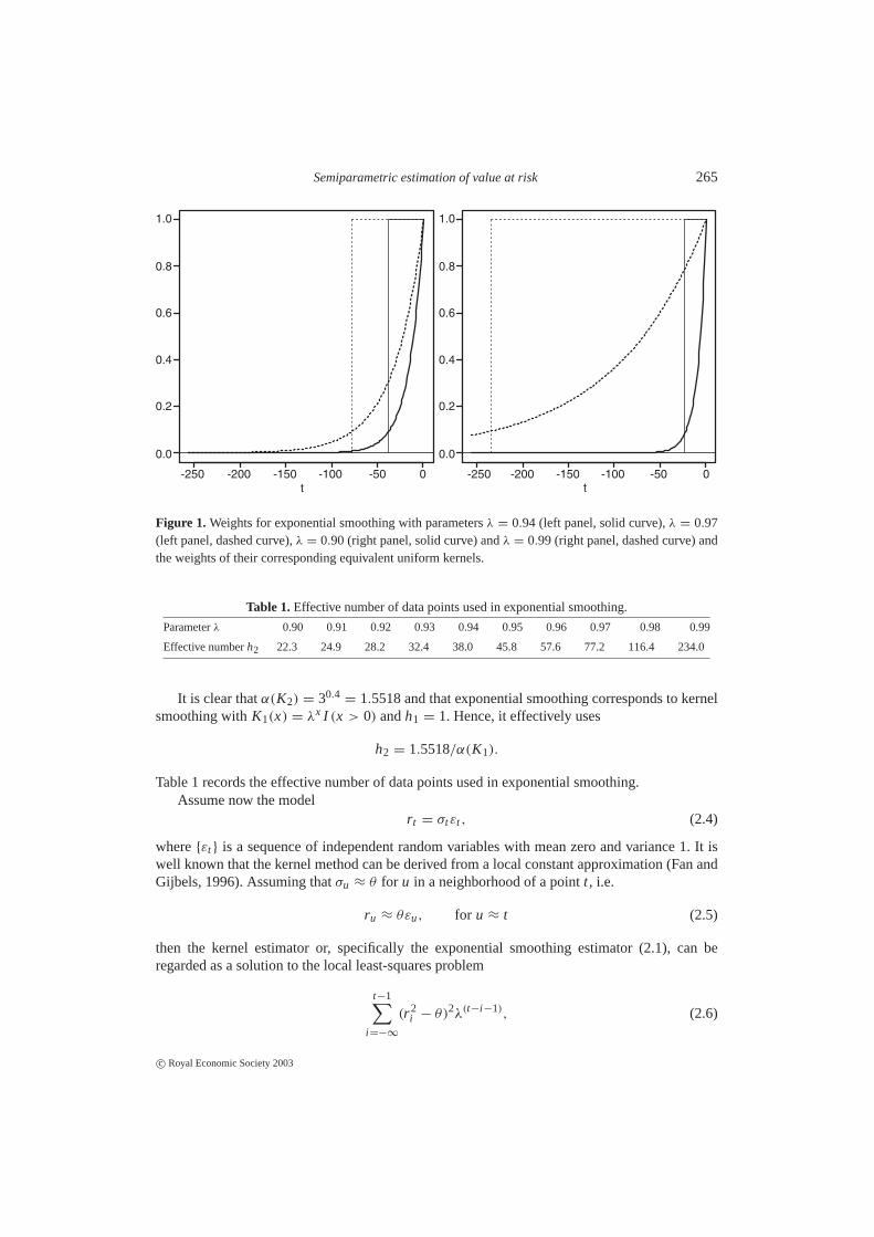
This is an example of exponential smoothing in the time domain (see Fan and Yao (2003)).Figure 1 depicts the weights for several choices ofλ.
Exponential smoothing can be regarded as a kernel method that uses the one-sided kernelK1(x) = bx I (x > 0) with b < 1. AssumingE(r t |�t−1) = 0, thenσ 2
t = E(r 2t |�t−1). The
kernel estimator ofσ 2t = E(r 2
t |�t−1) is given by
σ 2t =
∑t−1i =−∞
K1((t − i )/h1)r 2i∑t−1
i =−∞K1((t − i )/h1)
=
∑t−1i =−∞
bt−ih1 r 2
i∑t−1i =−∞
bt−ih1
,
whereh1 is the bandwidth (see Fan and Yao (2003)). It is clear that this is exactly the same as(2.3) withλ = b1/h1.
Exponential smoothing has the advantage of gradually, rather than radically, reducing theinfluence of remote data points. However, the effective number of points used in computing thelocal average is hard to quantify. If the one-sided uniform kernelK2(x) = I [0 < x ≤ 1] withbandwidthh2 is used, then it is clear that there areh2 data points used in computing the localaverage. According to the equivalent kernel theory (Section 5.4 of Fan and Yao (2003)), thekernel estimator with kernel functionK1 and bandwidthh1 and the kernel estimator with kernelfunction K2 and bandwidthh2 conduct approximately the same amount of smoothing when
h2 = α(K2)h1/α(K1),
where
α(K ) =
{∫∞
−∞
u2K (u)du
}−2/5{∫ ∞
−∞
K 2(u)du
}1/5
.
c© Royal Economic Society 2003
Semiparametric estimation of value at risk 265
t-250 -200 -150 -100 -50 0 0
t-250 -200 -150 -100 -50
1.0
0.8
0.6
0.4
0.2
0.0
1.0
0.8
0.6
0.4
0.2
0.0
Figure 1. Weights for exponential smoothing with parametersλ = 0.94 (left panel, solid curve),λ = 0.97(left panel, dashed curve),λ = 0.90 (right panel, solid curve) andλ = 0.99 (right panel, dashed curve) andthe weights of their corresponding equivalent uniform kernels.
Table 1.Effective number of data points used in exponential smoothing.
Parameterλ 0.90 0.91 0.92 0.93 0.94 0.95 0.96 0.97 0.98 0.99
Effective numberh2 22.3 24.9 28.2 32.4 38.0 45.8 57.6 77.2 116.4 234.0
It is clear thatα(K2) = 30.4= 1.5518 and that exponential smoothing corresponds to kernel
smoothing withK1(x) = λx I (x > 0) andh1 = 1. Hence, it effectively uses
h2 = 1.5518/α(K1).
Table 1 records the effective number of data points used in exponential smoothing.Assume now the model
r t = σtεt , (2.4)
where{εt } is a sequence of independent random variables with mean zero and variance 1. It iswell known that the kernel method can be derived from a local constant approximation (Fan andGijbels, 1996). Assuming thatσu ≈ θ for u in a neighborhood of a pointt , i.e.
ru ≈ θεu, for u ≈ t (2.5)
then the kernel estimator or, specifically the exponential smoothing estimator (2.1), can beregarded as a solution to the local least-squares problem
t−1∑i =−∞
(r 2i − θ)2λ(t−i −1), (2.6)
c© Royal Economic Society 2003

266 Jianqing Fan and Juan Gu
whereλ is a decay factor (smoothing parameter) that controls the size of the local neighborhood(Figure 1).
From the above function approximation point of view, the J. P. Morgan estimator of volatilityassumes that locally the return process follows the model (2.5). The model can, therefore, be re-garded as a discretized version of geometric Brownian motion with no drift,d log(Su) = θdWu,for u aroundt or
d log(Su) = θ(u)dWu, (2.7)
when the time unit is small, whereWu is the Wiener process.
2.2. Semiparametric models
The implicit assumption of J. P. Morgan’s estimation of volatility is the local geometric Brownianmotion stock price dynamics. To reduce possible modeling bias and to enhance the flexibility ofthe approximation, we enlarge the model (2.7) to the following semiparametric time-dependentmodel:
d log(Su) = θ(u)Sβ(u)u dWu, (2.8)
allowing volatility to depend on the value of asset, whereθ(u) and β(u) are the coefficientfunctions. Whenβ(u) ≡ 0, the model reduces to (2.7). This time-dependent diffusion modelwas used for interest rate dynamics by Fanet al. (2003). It is an extension of the time-dependentmodels previously considered by, among others, Hull and White (1990), Blacket al.(1990), andBlack and Karasinski (1991) and the time-independent model considered by Coxet al. (1985)and Chanet al. (1992). Unlike the yields of bonds, the scale of{Su} can be very different over alarge time period. However, the model (2.8) is used locally, rather than globally.
Motivated by the continuous-time model (2.8), we model the return process discrete time as
ru = θ(u)Sβ(u)
u−1 εu, (2.9)
whereεu is a sequence of independent random variables with mean 0 and variance 1. To estimatethe parametersθ(u) andβ(u), the local pseudo-likelihood technique is employed. For each givent andu ≤ t in a neighborhood of timet , the functionsθ(u) andβ(u) are approximated by theconstants
θ(u) ≈ θ, β(u) ≈ β.
Then, the conditional log-likelihood forru givenSu−1 is
−1
2log(2πθ2S2β
u−1) −r 2u
2θ2S2β
u−1
,
whenεu ∼ N(0, 1). In general, the above likelihood is a pseudo-likelihood. Dropping the con-stant factors and adding the pseudo-likelihood around the pointt , we obtain the locally weightedpseudo-likelihood
`(θ, β) = −
t−1∑i =−∞
{log(θ2S2β
i −1) +r 2i
θ2S2β
i −1
}λt−1−i , (2.10)
c© Royal Economic Society 2003

Semiparametric estimation of value at risk 267
whereλ < 1 is the decay factor that makes this pseudo-likelihood use only the local data (seeFigure 1 and (2.6)). Maximizing (2.10) with respect to the local parametersθ andβ yields anestimate of the local parametersθ(t) andβ(t). Note that for givenβ, the maximum is achieved at
θ2(t, β) = (1 − λ)
t−1∑i =−∞
λt−1−i r 2i S−2β
i −1 .
Substituting this into (2.10), the pseudo-likelihood(θ(t, β), β) is obtained. This is aone-dimensional maximization problem, and the maximization can easily be obtained by, forexample, searchingβ over a grid of points or by using other more advanced numerical methods.Let β(t) be the maximizer. Then, the estimated volatility for the one-period return is
σ 2t = θ2(t)S2β(t)
t−1 , (2.11)
whereθ (t) = θ (t, β(t)). In particular, if we letβ(t) = 0, the model (2.9) becomes the model(2.7) and the estimator (2.11) reduces to the J. P. Morgan estimator (2.3).
Our method corresponds to time-domain smoothing, which uses mainly the most recent data.There is also a large literature that postulates models on Var(r t |F t−1) = g(r t−1, . . . , r t−p).This corresponds to the state-domain smoothing, using mainly the historical data to estimate thefunctiong. See Engle and Manganelli (2000), Yanget al.(1999), Yatchew and Hardle (2003) andFan and Yao (2003). Combination of both time-domain and state-domain smoothing for volatilityestimation is an interesting direction for future research.
2.3. Choice of decay factor
The performance of volatility estimation depends on the choice of decay factorλ. In the Risk-Metrics, λ = 0.94 is recommended for the estimation of 1-day volatility, whileλ = 0.97 isrecommended for the estimation of monthly volatility. In general, the choice of decay factorshould depend on the portfolio and holding period, and should be determined from the data.
Our idea is related to minimizing the prediction error. In the current pseudo-likelihoodestimation context, our aim is to maximize the pseudo-likelihood. For example, suppose thatwe have observed the price processSt , t = 1, . . . , T . Note that the pseudo-likelihood estima-tor σ 2
t depends on the data up to timet − 1. This estimated volatility can be used to predictthe volatility at timet . The estimated volatilityσ 2
t given by (2.11) can then be compared withthe observed volatilityr 2
t to assess the effectiveness of the estimation. One way to validate theeffectiveness of the prediction is to use square prediction errors
PE(λ) =
T∑t=T0
(r 2t − σ 2
t )2, (2.12)
whereT0 is an integer such thatσ 2T0
can be estimated with reasonable accuracy. This avoids theboundary problem caused by the exponential smoothing (2.1) or (2.3). The decay factorλ canbe chosen to minimize (2.12). Using the model (2.9) and noting thatσt is �t−1 measurable, theexpected value can be decomposed as
E{PE(λ)} =
T∑t=T0
E(σ 2t − σ 2
t )2+
T∑t=T0
E(r 2t − σ 2
t )2. (2.13)
c© Royal Economic Society 2003
268 Jianqing Fan and Juan Gu
Note that the second term is independent ofλ. Thus, minimizing PE(λ) aims at finding an esti-mator that minimizes the mean-square error
T∑t=T0
E(σ 2t − σ 2
t )2.
A question arises naturally why square errors, rather than, other types of errors, such asabsolute deviation errors should be used in (2.12). In the current pseudo-likelihood context, anatural alternative is to maximize the pseudo-likelihood defined as
PL(λ) = −
T∑t=T0
(log σ 2t + r 2
t /σ 2t ), (2.14)
compared to (2.10). The likelihood function is a natural measure of the discrepancy betweenr t
andσt in the current context, and does not depend on an arbitrary choice of distance. The sum-mand in (2.14) is the conditional likelihood, after dropping constant terms, ofr t givenSt−1 withunknown parameters replaced by their estimated values. The decay factorλ can then be chosento maximize (2.14). For simplicity in later discussion, we call this procedure semiparametricestimation of volatility (SEV).
2.4. Choice of adaptive smoothing parameter
The above choice of decay factor remains constant during post-sample forecasting. It relies heav-ily on the past history and has little flexibility to accommodate changes in stock dynamics overtime. Therefore, in order to adapt automatically to changes in stock price dynamics, the decayingparameterλ should be allowed to depend on the timet . A solution to such problems has beenexplored by Mercurio and Spokoiny (2003) and Hardleet al. (2003).
To highlight possible changes of the dynamics of{St }, the validation should be localizedaround the current timet . Let g be a period for which we wish to validate the effectiveness ofvolatility estimation. Then, the pseudo-likelihood is defined as
PL(λ, t) = −
t−1∑i =t−1−g
(log σ 2i + r 2
i /σ 2i ). (2.15)
Let λt maximize (2.15). In our implementation, we useg = 20, which validates the estimates ina period of about 1 month. The choice ofλt is variable. To reduce this variability, the series{λt }
can be smoothed further by using the exponential smoothing
3t = b3t−1 + (1 − b)λt . (2.16)
In our implementation, we useb = 0.94.To sum up, in order to estimate the volatilityσt , we first compute{σu} and{3u} up to time
t − 1 and obtainλt by minimizing (2.15) and then3t from (2.16). The value of3t is then usedin (2.10) to estimate the local parametersθ (t) andβ(t), and hence the volatilityσ 2
t using (2.11).The resulting estimator will be referred to as the adaptive volatility estimator (AVE).
The techniques in this section and Section 2.3 apply directly to the J. P. Morgan type ofestimator (2.1). This allows different decay parameters for different portfolios.
c© Royal Economic Society 2003
Semiparametric estimation of value at risk 269
2.5. Numerical results
In this section, the newly proposed procedures are compared by using three commonly usedmethods: RiskMetrics, historical simulation and a GARCH model using the quasi-maximumlikelihood method (denoted by ‘GARCH’). See Engle and Gonzalez-Rivera (1991) and Boller-slev and Wooldridge (1992). For the estimation of volatility, the historical simulation methodis simply defined as the sample standard deviation of the return process for the past 250 days.For the newly proposed method, we employ the semiparametric estimator (2.11) withλ = 0.94(denoted by ‘semipara’); the estimator (2.11) withλ chosen by minimizing (2.12) (denoted by‘SEV’); and the estimator (2.11) (denoted by ‘AVE’) with the decay factor3t chosen adaptivelyas in (2.16).
To compare the different procedures for estimating the volatility with a holding period of1 day, eight stock indices and two simulated data sets were used together with the following fiveperformance measures. For other related measures, see Dave and Stahl (1997). For a holdingperiod of 1 day, the error distribution is not very far from normal.
Measure 1 (Exceedance ratio against confidence level).This measure counts number of eventsfor which the loss of the asset exceeds the loss predicted by the normal model at a given con-fidenceα. With estimated volatility, under the normal model, the 1-day VaR is estimated by8−1(α)σt , where8−1(α) is theα quantile of the standard normal distribution. For each esti-mated VaR, the exceedance ratio (ER) is computed as
ER = n−1T+n∑
t=T+1
I (r t < 8−1(α)σt ),
for a post sample of sizen. This gives an indication of how effectively volatility can be used forestimating one-period VaR. Note that the Monte Carlo error for this measure has an approximatesize{α(1 − α)/n}
1/2, even when the trueσt is used. For example, withα = 5% andn = 1000,the Monte Carlo error is around 0.68%. Thus, unless the post-sample size is large enough, thismeasure has difficulty in differentiating between various estimators due to the presence of largeerror margins.
Measure 2 (Mean absolute deviation error, MADE).To motivate this measure, let us firstconsider the mean square errors
PE= n−1T+n∑
t=T+1
(r 2t − σ 2
t )2.
Following (2.13), the expected value can be decomposed as
E(PE) = n−1T+n∑
t=T+1
E(σ 2t − σ 2
t )2+ n−1
T+n∑t=T+1
E(r 2t − σ 2
t )2.
Note that the first term reflects the effectiveness of the estimated volatility while the secondterm is the size of the stochastic error, independent of estimators. As in all statistical predictionproblems, the second term is usually of an order of magnitude larger than the first term. Thus,
c© Royal Economic Society 2003
270 Jianqing Fan and Juan Gu
a small improvement on PE could mean substantial improvement over the estimated volatility.However, due to the well-known fact that financial time series contain outliers due to marketcrashes, the mean-square error is not a robust measure. Therefore, we will use the mean-absolutedeviation error
MADE = n−1T+n∑
t=T+1
|r 2t − σ 2
t |.
Measure 3 (Square-root absolute deviation error, RADE).An alternative variation to MADEis the RADE, which is defined as
RADE = n−1T+n∑
t=T+1
∣∣∣∣∣|r t | −
√2
πσt
∣∣∣∣∣.The constant factor comes from the fact thatE|εt | =
√2π
for εt ∼ N(0, 1).
Measure 4—Test of independence.A good VaR estimator should have the property that thesequence of the events exceeding VaR behaves like ani.i.d. Bernoulli distribution with probabil-ity of successα. Engle and Manganelli (1999) give an illuminating example showing that even abad VaR estimator can have the right exceedance ratioα.
Let I t = I (r t < 8−1(α)σt ) be the indicator of the event that the return exceeds VaR.Christoffersen (1998) introduced the likelihood ratio test for testing independence and for testingwhether the probability Pr(I t = 1) = α.
Assume{I t } is a first-order Markovian chain. Letπi j = Pr(I t = j |I t−1 = i ) (i = 0, 1 andj = 0, 1) be the transition probability andni j be the number of events transferring from stateito statej in the post-sample period. The problem is to test
H0 : π00 = π10 = π, π01 = π11 = 1 − π.
Then the maximum likelihood ratio test for independence is
LR1 = 2 log
(π
n0000 π
n0101 π
n1010 π
n1111
πn0(1 − π)n1
), (2.17)
whereπi j = ni j /(ni 0 + ni,1), n j = n0 j + n1 j , and π = n0/(n0 + n1). The test statistic isa measure of deviation from independence. Under the null hypothesis, the test statistic LR1 isdistributed approximately according toχ2
1 when sample size is large. Thus, reporting the teststatistic is equivalent to reporting theP-value.
Measure 5—Testing against a given confidence level.Christoffersen (1998) applied the max-imum likelihood ratio test to the problem
H0 : P(I t = 1) = α vs. H1 : P(I t = 1) 6= α
under the assumption that{I t } is a sequence ofi.i.d. Bernoulli random variables. The test statisticis given by
LR2 = 2 log
(πn0(1 − π)n1
αn0(1 − α)n1
), (2.18)
which follows theχ21 -distribution when the sample size is large. Again, theP-value is a measure
of deviation from the null hypothesis, which is closely related to the ER.
c© Royal Economic Society 2003
Semiparametric estimation of value at risk 271
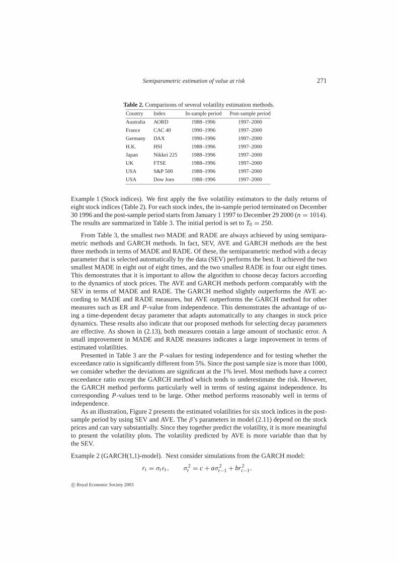
Table 2.Comparisons of several volatility estimation methods.
Country Index In-sample period Post-sample period
Australia AORD 1988–1996 1997–2000
France CAC 40 1990–1996 1997–2000
Germany DAX 1990–1996 1997–2000
H.K. HSI 1988–1996 1997–2000
Japan Nikkei 225 1988–1996 1997–2000
UK FTSE 1988–1996 1997–2000
USA S&P 500 1988–1996 1997–2000
USA Dow Joes 1988–1996 1997–2000
Example 1 (Stock indices).We first apply the five volatility estimators to the daily returns ofeight stock indices (Table 2). For each stock index, the in-sample period terminated on December30 1996 and the post-sample period starts from January 1 1997 to December 29 2000 (n = 1014).The results are summarized in Table 3. The initial period is set toT0 = 250.
From Table 3, the smallest two MADE and RADE are always achieved by using semipara-metric methods and GARCH methods. In fact, SEV, AVE and GARCH methods are the bestthree methods in terms of MADE and RADE. Of these, the semiparametric method with a decayparameter that is selected automatically by the data (SEV) performs the best. It achieved the twosmallest MADE in eight out of eight times, and the two smallest RADE in four out eight times.This demonstrates that it is important to allow the algorithm to choose decay factors accordingto the dynamics of stock prices. The AVE and GARCH methods perform comparably with theSEV in terms of MADE and RADE. The GARCH method slightly outperforms the AVE ac-cording to MADE and RADE measures, but AVE outperforms the GARCH method for othermeasures such as ER andP-value from independence. This demonstrates the advantage of us-ing a time-dependent decay parameter that adapts automatically to any changes in stock pricedynamics. These results also indicate that our proposed methods for selecting decay parametersare effective. As shown in (2.13), both measures contain a large amount of stochastic error. Asmall improvement in MADE and RADE measures indicates a large improvement in terms ofestimated volatilities.
Presented in Table 3 are theP-values for testing independence and for testing whether theexceedance ratio is significantly different from 5%. Since the post sample size is more than 1000,we consider whether the deviations are significant at the 1% level. Most methods have a correctexceedance ratio except the GARCH method which tends to underestimate the risk. However,the GARCH method performs particularly well in terms of testing against independence. ItscorrespondingP-values tend to be large. Other method performs reasonably well in terms ofindependence.
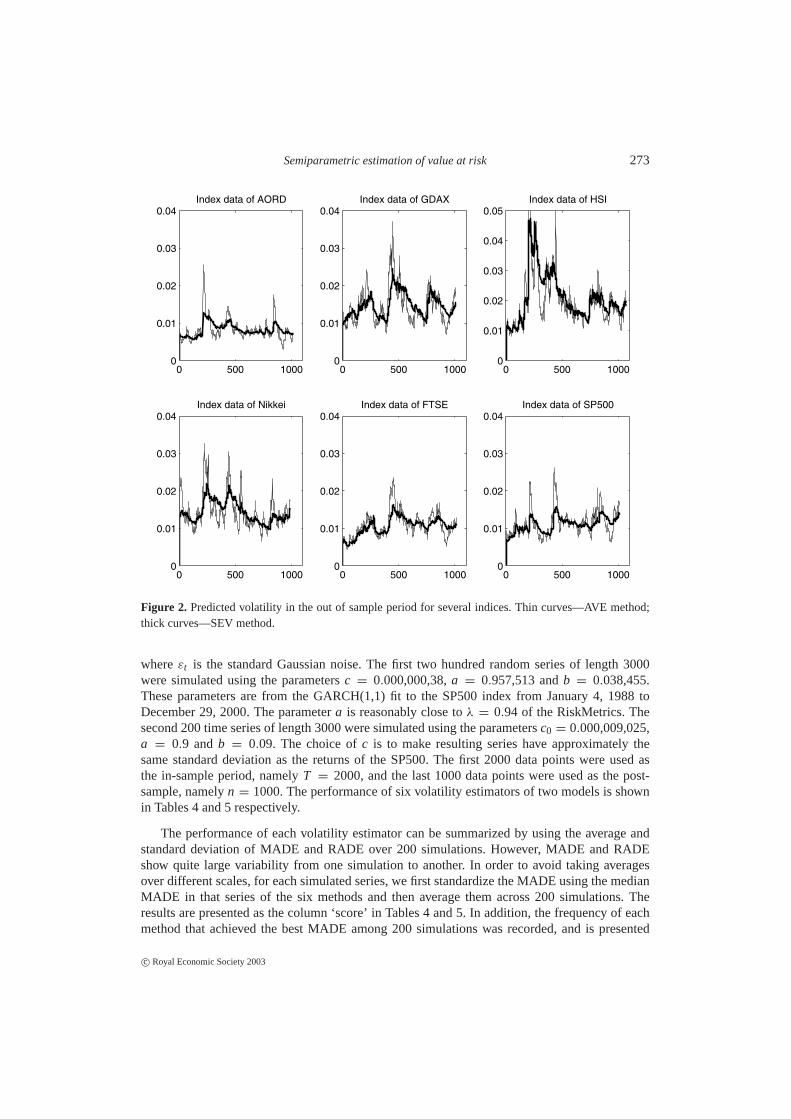
As an illustration, Figure 2 presents the estimated volatilities for six stock indices in the post-sample period by using SEV and AVE. Theβ ’s parameters in model (2.11) depend on the stockprices and can vary substantially. Since they together predict the volatility, it is more meaningfulto present the volatility plots. The volatility predicted by AVE is more variable than that bythe SEV.
Example 2 (GARCH(1,1)-model).Next consider simulations from the GARCH model:
r t = σtεt , σ 2t = c + aσ 2
t−1 + br2t−1,
c© Royal Economic Society 2003

272 Jianqing Fan and Juan Gu
Table 3.Comparisons of several volatility estimation methods.Index Method ER MADE RADE P-value P-value
(×10−2) (×10−4) (×10−3) (indep) (ER= 5%)Historical 5.23 0.85 4.33 0.01a 0.76RiskMetrics 4.93 0.848 4.25 0.01a 0.92
AORD Semipara 4.93 0.84 4.231 0.01a 0.92SEV 5.23 0.803 4.30 0.02 0.76AEV 4.93 0.835 4.213 0.00a 0.92GARCH 5.52 0.786 4.168 0.12 0.46
Historical 6.16 2.177 7.272 0.11 0.10RiskMetrics 6.36 2.157 7.102 0.33 0.06
CAC 40 Semipara 6.55 2.15 7.094 0.20 0.03SEV 6.45 2.077 7.035 0.17 0.04AEV 6.36 2.138 7.069 0.91 0.06GARCH 8.24 1.931 6.883 0.20 0.00
Historical 6.55 2.507 7.814 0.18 0.03RiskMetrics 5.46 2.389 7.37 0.59 0.51
DAX Semipara 5.56 2.389 7.342 0.90 0.43SEV 6.06 2.368 7.457 0.03 0.14AEV 5.96 2.377 7.330 0.90 0.18GARCH 7.94 2.200 7.174 0.78 0.00a
Historical 6.08 5.71 11.167 0.00a 0.12RiskMetrics 5.99 5.686 10.818 0.00a 0.15
HSI Semipara 5.89 5.567 10.685 0.00a 0.19SEV 5.61 5.523 10.743 0.00a 0.37AEV 6.55 5.578 10.686 0.00a 0.03GARCH 7.3 5.293 10.565 0.03 0.00a
Historical 5.78 2.567 7.824 0.90 0.27RiskMetrics 5.78 2.526 7.656 0.35 0.27
Nikkei 225 Semipara 6.09 2.507 7.631 0.48 0.13SEV 5.68 2.457 7.610 0.68 0.34AEV 6.19 2.479 7.565 0.25 0.10GARCH 5.88 2.563 7.693 0.80 0.22
Historical 6.83 1.369 5.761 0.05 0.01RiskMetrics 5.94 1.342 5.594 0.45 0.18
FTSE Semipara 6.24 1.328 5.567 0.58 0.08SEV 6.93 1.299 5.598 0.02 0.01AEV 6.04 1.328 5.571 0.90 0.14GARCH 7.43 1.256 5.497 0.78 0.00a
Historical 6.34 1.613 6.027 0.65 0.06RiskMetrics 5.55 1.647 6.056 0.62 0.44
S&P 500 Semipara 5.55 1.62 5.995 0.62 0.44SEV 5.85 1.539 5.888 0.46 0.23AEV 5.75 1.611 5.984 0.51 0.29GARCH 4.46 1.689 6.163 0.89 0.43
Historical 6.15 1.493 5.84 0.25 0.11RiskMetrics 5.65 1.507 5.784 0.56 0.35
Dow Jones Semipara 5.75 1.489 5.739 0.16 0.29SEV 5.75 1.460 5.743 0.51 0.29AEV 5.85 1.480 5.731 0.90 0.23GARCH 4.46 1.575 5.96 0.68 0.43
Note: GARCH refers to the GARCH(1,1) model. Numbers with bold face are the two smallest.a Means statistically significant at the 1% level.
c© Royal Economic Society 2003
Semiparametric estimation of value at risk 273
0 500 10000
0.01
0.02
0.03
0.04Index data of AORD
0 500 10000
0.01
0.02
0.03
0.04Index data of GDAX
0 500 10000
0.01
0.02
0.03
0.04
0.05Index data of HSI
0 500 10000
0.01
0.02
0.03
0.04Index data of Nikkei
0 500 10000
0.01
0.02
0.03
0.04Index data of FTSE
0 500 10000
0.01
0.02
0.03
0.04Index data of SP500
Figure 2. Predicted volatility in the out of sample period for several indices. Thin curves—AVE method;thick curves—SEV method.
whereεt is the standard Gaussian noise. The first two hundred random series of length 3000were simulated using the parametersc = 0.000,000,38,a = 0.957,513 andb = 0.038,455.These parameters are from the GARCH(1,1) fit to the SP500 index from January 4, 1988 toDecember 29, 2000. The parametera is reasonably close toλ = 0.94 of the RiskMetrics. Thesecond 200 time series of length 3000 were simulated using the parametersc0 = 0.000,009,025,a = 0.9 andb = 0.09. The choice ofc is to make resulting series have approximately thesame standard deviation as the returns of the SP500. The first 2000 data points were used asthe in-sample period, namelyT = 2000, and the last 1000 data points were used as the post-sample, namelyn = 1000. The performance of six volatility estimators of two models is shownin Tables 4 and 5 respectively.
The performance of each volatility estimator can be summarized by using the average andstandard deviation of MADE and RADE over 200 simulations. However, MADE and RADEshow quite large variability from one simulation to another. In order to avoid taking averagesover different scales, for each simulated series, we first standardize the MADE using the medianMADE in that series of the six methods and then average them across 200 simulations. Theresults are presented as the column ‘score’ in Tables 4 and 5. In addition, the frequency of eachmethod that achieved the best MADE among 200 simulations was recorded, and is presented
c© Royal Economic Society 2003
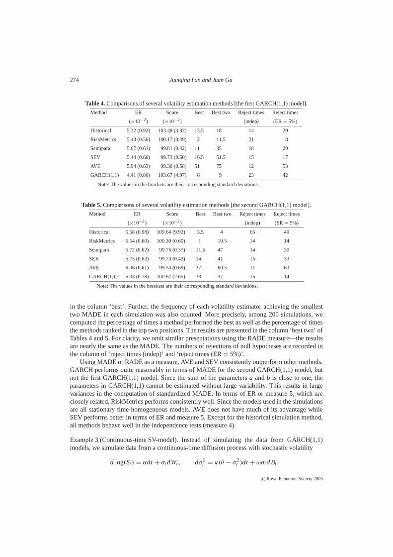
274 Jianqing Fan and Juan Gu
Table 4.Comparisons of several volatility estimation methods [the first GARCH(1,1) model].
Method ER Score Best Best two Reject times Reject times
(×10−2) (×10−2) (indep) (ER= 5%)
Historical 5.32 (0.92) 103.48 (4.87) 13.5 18 14 29
RiskMetrics 5.43 (0.56) 100.17 (0.49) 2 11.5 21 8
Semipara 5.67 (0.61) 99.81 (0.42) 11 35 18 20
SEV 5.44 (0.66) 99.73 (0.50) 16.5 51.5 15 17
AVE 5.94 (0.63) 99.30 (0.58) 51 75 12 53
GARCH(1,1) 4.41 (0.86) 103.67 (4.97) 6 9 23 42
Note: The values in the brackets are their corresponding standard deviations.
Table 5.Comparisons of several volatility estimation methods [the second GARCH(1,1) model].
Method ER Score Best Best two Reject times Reject times
(×10−2) (×10−2) (indep) (ER= 5%)
Historical 5.58 (0.98) 109.64 (9.92) 3.5 4 65 49
RiskMetrics 5.54 (0.60) 100.30 (0.60) 1 10.5 14 14
Semipara 5.72 (0.62) 99.75 (0.37) 11.5 47 14 30
SEV 5.75 (0.62) 99.73 (0.42) 14 41 15 33
AVE 6.06 (0.61) 99.53 (0.69) 37 60.5 11 63
GARCH(1,1) 5.03 (0.78) 100.67 (2.65) 33 37 15 14
Note: The values in the brackets are their corresponding standard deviations.
in the column ‘best’. Further, the frequency of each volatility estimator achieving the smallesttwo MADE in each simulation was also counted. More precisely, among 200 simulations, wecomputed the percentage of times a method performed the best as well as the percentage of timesthe methods ranked in the top two positions. The results are presented in the column ‘best two’ ofTables 4 and 5. For clarity, we omit similar presentations using the RADE measure—the resultsare nearly the same as the MADE. The numbers of rejections of null hypotheses are recorded inthe column of ‘reject times (indep)’ and ‘reject times (ER= 5%)’.
Using MADE or RADE as a measure, AVE and SEV consistently outperform other methods.GARCH performs quite reasonably in terms of MADE for the second GARCH(1,1) model, butnot the first GARCH(1,1) model. Since the sum of the parametersa andb is close to one, theparameters in GARCH(1,1) cannot be estimated without large variability. This results in largevariances in the computation of standardized MADE. In terms of ER or measure 5, which areclosely related, RiskMetrics performs consistently well. Since the models used in the simulationsare all stationary time-homogeneous models, AVE does not have much of its advantage whileSEV performs better in terms of ER and measure 5. Except for the historical simulation method,all methods behave well in the independence tests (measure 4).
Example 3 (Continuous-time SV-model).Instead of simulating the data from GARCH(1,1)models, we simulate data from a continuous-time diffusion process with stochastic volatility
d log(St ) = αdt + σtdWt , dσ 2t = κ(θ − σ 2
t )dt + ωσtd Bt ,
c© Royal Economic Society 2003
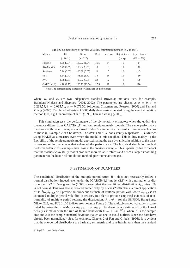
Semiparametric estimation of value at risk 275
Table 6.Comparisons of several volatility estimation methods (SV model).
Method ER Score Best Best two Reject times Reject times
(×10−2) (×10−2) (indep) (ER= 5%)
Historic 5.05 (0.74) 100.02 (1.94) 16.5 34 5 14
RiskMetrics 5.45 (0.59) 100.62 (0.59) 0 3 11 12
Semipara 5.90 (0.65) 100.38 (0.67) 0 5 10 45
SEV 5.64 (0.71) 98.69 (1.42) 34 66 11 30
AVE 6.06 (0.63) 99.02 (0.64) 32 72 8 60
GARCH(1,1) 4.10 (1.77) 108.73 (13.54) 17.5 20 9 116
Note: The corresponding standard deviations are in the brackets.
where Wt and Bt are two independent standard Brownian motions. See, for example,Barndorff-Nielsen and Shephard (2001, 2002). The parameters are chosen asα = 0, κ =
0.214,59,θ = 0.085,71,ω = 0.078,30, following Chapman and Pearson (2000) and Fan andZhang (2003). Two hundred series of 3000 daily data were simulated using the exact simulationmethod (see, e.g. Genon-Catalotet al. (1999), Fan and Zhang (2003)).
This simulation tests the performance of the six volatility estimators when the underlyingdynamics differs from GARCH(1,1) and our semiparametric models. The same performancemeasures as those in Example 2 are used. Table 6 summarizes the results. Similar conclusionsto those in Example 2 can be drawn. The AVE and SEV consistently outperform RiskMetricsusing MADE as a measure even when the model is mis-specified. This is due, mainly, to theflexibility of the semiparametric model approximating the true dynamics, in addition to the data-driven smoothing parameter that enhanced the performance. The historical simulation methodperforms better in this example than those in the previous example. This is partially due to the factthat the stochastic volatility model produces more volatile returns and hence a larger smoothingparameter in the historical simulation method gives some advantages.
3. ESTIMATION OF QUANTILES
The conditional distribution of the multiple period returnRt,τ does not necessarily follow anormal distribution. Indeed, even under the IGARCH(1,1) model (2.1) with a normal error dis-tribution in (2.4), Wong and So (2003) showed that the conditional distributionRt,τ given �t
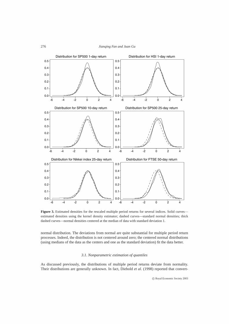
is not normal. This was also illustrated numerically by Lucas (2000). Thus, a direct applicationof 8−1(α)σt+1,τ will provide an erroneous estimate of multiple period VaR, whereσt+1,τ is anestimated multiple period volatility of returns. In order to provide empirical evidence of non-normality of multiple period returns, the distributionsRt,τ /σt,τ for the S&P500, Hang-Seng,Nikkei 225, and FTSE 100 indices are shown in Figure 3. The multiple period volatility is com-puted by using the RiskMetricsσt+1,τ =
√τ σt+1. The densities are estimated by the kernel
density estimator with the rule of thumb bandwidthh = 1.06n−1/5s, wheren is the samplesize ands is the sample standard deviation (taken as one to avoid outliers, since the data havealready been normalized). See, for example, Chapter 2 of Fan and Gijbels (1996). It is evidentthat the one-period distributions are basically symmetric and have heavier tails than the standard
c© Royal Economic Society 2003
276 Jianqing Fan and Juan Gu
-6 -4 -2 0 2 4 -6 -4 -2 0 2 4
-6 -4 -2 0 2 4 -6 -4 -2 0 2 4
-6 -4 -2 0 2 4 -6 -4 -2 0 2 4
Distribution for SP500 1-day return Distribution for HSI 1-day return
Distribution for SP500 10-day return Distribution for SP500 25-day return
Distribution for Nikkei index 25-day return Distribution for FTSE 50-day return
0.5
0.4
0.3
0.2
0.1
0.0
0.5
0.4
0.3
0.2
0.1
0.0
0.5
0.4
0.3
0.2
0.1
0.0
0.5
0.4
0.3
0.2
0.1
0.0
0.5
0.4
0.3
0.2
0.1
0.0
0.5
0.4
0.3
0.2
0.1
0.0
Figure 3. Estimated densities for the rescaled multiple period returns for several indices. Solid curves—estimated densities using the kernel density estimator; dashed curves—standard normal densities; thickdashed curves—normal densities centered at the median of data with standard deviation 1.
normal distribution. The deviations from normal are quite substantial for multiple period returnprocesses. Indeed, the distribution is not centered around zero; the centered normal distributions(using medians of the data as the centers and one as the standard deviation) fit the data better.
3.1. Nonparametric estimation of quantiles
As discussed previously, the distributions of multiple period returns deviate from normality.Their distributions are generally unknown. In fact, Dieboldet al. (1998) reported that convert-
c© Royal Economic Society 2003

Semiparametric estimation of value at risk 277
ing 1-day volatility estimates toτ -day estimates by a scale factor√
τ is inappropriate and pro-duces overestimates of the variability of long time horizon volatility. Danielsson and de Vries(2000) suggested using the scaling factorτ1/β with β being the tail index of extreme valuedistributions. Nonparametric methods can naturally be used to estimate the distributions of theresiduals and correct the biases in the volatility estimation (the issue of whether the scale fac-tor is correct becomes irrelevant when estimating the distribution of standardized return pro-cesses).
Let σt,τ be an estimatedτ -period volatility andεt,τ = Rt,τ /σt,τ be a residual. Denote byq(α, τ ), the sampleα-quantile of the residuals{εt,τ , t = T0 + 1, . . . , T − τ }. This yields anestimated multiple period VaR as VaRt+1,τ = q(α, τ )σt+1,τ . Note that the choice of constantfactor q(α, τ ) is the same as selecting the constant factorc such that the difference between theexceedance ratio of the estimated VaR and confidence level is minimized in the in-sample period.More precisely,q(α, τ ) minimizes the function
ER(c) =
∣∣∣∣(T − τ − T0 + 1)−1T−τ∑t=T0
I (Rt+1,τ < cσt+1,τ ) − α
∣∣∣∣.The nonparametric estimates of quantiles are robust against the possible mis-specification of
parametric models and insensitive to a few large market movements for moderateα. Yet, they arenot as efficient as parametric methods when parametric models are correctly given. To improvethe efficiency of nonparametric estimates, we assume the distribution of{εt,τ } is symmetric aboutthe point 0. This implies that
q(α, τ ) = −q(1 − α, τ),
whereq(α, τ ) is the population quantile. Thus, an improved nonparametric estimator is
q[1](α, τ ) = 2−1{q(α, τ ) − q(1 − α, τ)}. (3.1)
Denote by
VaR[1]
t+1,τ = q(α, τ )[1]σt+1,τ
the corresponding estimated VaR. It is not difficult to show that the estimatorq[1](α, τ ) is a factor(2− 2α)/(1− 2α) as efficient as the simple estimateq(α, τ ) for α < 0.5 (see Appendix A.1 forderivations).
When the distribution of the standardized return process is asymmetric, (3.1) will introducesome biases. For moderateα whereq(α, τ ) ≈ −q(1−α, τ), the biases are offset by the variancegain. As shown in Figure 3, the asymmetry for returns is not very severe for moderateα. Hence,the gain can still be materialized.
3.2. Adaptive estimation of quantiles
The above method assumes that the distribution of{εt,τ } is stationary over time. To accommodatepossible nonstationarity, for a given timet , we may use only the local data{εi,τ , i = t −τ −h, t −h + 1, . . . , t − τ }. This model was used by several authors, including Wong and So (2003) andPant and Chang (2001). Let the resulting nonparametric estimator (3.1) beq[1]
t (α, τ ). To stabilize
c© Royal Economic Society 2003

278 Jianqing Fan and Juan Gu
the estimated quantiles, we smooth further this quantile series to obtain the adaptive estimator ofquantilesq[2]
t (α, τ ) via the exponential smoothing
q[2]
t (α, τ ) = bq[2]
t−1(α, τ ) + (1 − b)q[1]
t−1(α, τ ). (3.2)
In our implementation, we tookh = 250 andb = 0.94.
3.3. Parametric estimation of quantiles
Based on empirical observations, one possible parametric model for the observed residuals{εt,τ ,
t = T0 + 1, . . . , T − τ } is to assume that the residuals follow a scaledt-distribution:
εt,τ = λε∗t , (3.3)
whereε∗t ∼ tν , the Student’st-distribution with degree of freedomν. The parametersλ andν
can be obtained by solving the following equations that are related to the sample quantiles:{q(α1, τ ) = λt (α1, ν)
q(α2, τ ) = λt (α2, ν),
wheret (α, ν) is theα quantile of thet-distribution with degree of freedomν. A better estimatorto use isq[1](α, τ ) in (3.1). Using the improved estimator and solving the above equations yieldsthe estimatesν andλ as follows:
t (α2, ν)
t (α1, ν)=
q[1](α2, τ )
q[1](α1, τ ), λ =
q[1](α1, τ )
t (α1, ν). (3.4)
Hence, the estimated quantile is given by
q[3](α, τ ) = λt (α, ν) =t (α, ν)q[1](α1, τ )
t (α1, ν). (3.5)
and the VaR ofτ -period return is given by
VaR[3]
t+1,τ = q[3](α, τ )σt+1,τ . (3.6)
In our implementation, we takeα1 = 0.15 andα2 = 0.35. This choice is near optimal in termsof statistical efficiency (Figure 4).
The above method of estimating quantiles is robust against outliers. An alternative approachis to use the method of moments to estimate the parameters in (3.3). Note that ifε ∼ tν withν > 4, then
Eε2=
ν
ν − 2and Eε4
=3ν2
(ν − 2)(ν − 4).
The method of moments yields the following estimates:{ν = (4µ4 − 6µ2
2)/(µ4 − 3µ22)
λ = {µ2(ν − 2)/ν}1/2,
(3.7)
c© Royal Economic Society 2003

Semiparametric estimation of value at risk 279
a
Efficiency of quantile estimation as a function of alpha
10
5
00.0 0.1 0.2 0.3 0.4
15
20
25
30
Figure 4. The efficiency functiongν(α) for degree of freedomν = 2, ν = 3, ν = 5, ν = 10 andν = 40(from solid, the shortest dash to the longest dash). For allν, the minimum is almost attained at the interval[0.1, 0.2].
whereµ j is the j th moment, defined asµ j = (T − τ − T0)−1∑T−τ
t=T0+1 εjt,τ . See Pant and
Chang (2001) for similar expressions. Using these estimated parameters, we obtain the new esti-mated quantile and estimated VaR similarly to (3.5) and (3.6). The new estimates are denoted byq[4](α, τ ) and VaR[4]
t+1,τ , respectively. That is,
q[4](α, τ ) = λt (α, ν), VaR[4]
t+1,τ = q[4](α, τ )σt+1,τ .
The method of moments is less robust than the method of quantiles. The former also requiresthe assumption thatν > 4. We will compare their asymptotic efficiency in Section 3.4.
3.4. Theoretical comparisons of estimators for quantiles
Of the three methods for estimating the quantiles, the estimatorq[1](α, τ ) is the most robustmethod. It imposes very mild assumptions on the distribution ofεt,τ and, hence, is robust againstmodel mis-specification. The two parametric methods rely on the model (3.3), which could leadto erroneous estimation if the model is mis-specified. The estimatorsq[1], q[2] and q[3] are allrobust against outliers, butq[4] is not.
In order to give a theoretical study on the properties of the aforementioned three methodsfor estimation of quantiles, we assume that{εt,τ , t = T0, . . . , T − τ } is an independent randomsample from the densityf . Under this condition, for 0< α1 < · · · < αk < 1,
{√
m[q(αi , τ ) − q(αi , τ )], 1 ≤ i ≤ k}L
−→ N(0, 6), (3.8)
wherem = T − τ − T0 + 1, q(αi , τ ) is the population quantile off , and6 = (σi j ) with
σi j = αi (1 − α j )/ f (q(αi , τ )) f (q(α j , τ )), for i > j andσ j i = σi j .
See Prakasa Rao (1987).To compare this with parametric methods, let us now assume for a moment that the model
(3.3) is correct. Using the result in Appendix A.1, the nonparametric estimatorq[1](α, τ ) follows
c© Royal Economic Society 2003

280 Jianqing Fan and Juan Gu
asymptotically a normal distribution with meanλt (α, ν) and variance (forα < 1/2)
V1(α, ν, λ) =λ2α(1 − 2α)
2 fν(t (α, ν))2m, (3.9)
where fν is the density of thet-distribution with degree of freedomν given by
fν(x) =0((ν + 1)/2)√
νπ0(ν/2)(1 + x2/ν)−(ν+1)/2.
Sinceν is an integer, any consistent estimator ofν is equal toν with probability tending toone. For this reason,ν can be treated as known in the asymptotic study. It follows directly from(3.8) that the estimatorq[3](α, τ ) has the asymptotic normal distribution with meanλt (α, ν) andvariance
V2(α, α1, ν, λ) =λ2t (α, ν)2α1(1 − 2α1)
2 fν(t (α1, ν))2t (α1, ν)2m. (3.10)
The efficiency ofV2 depends on the choice ofα1 through the function
gν(α) =α(1 − 2α)
fν(t (α, ν))2t (α, ν)2.
The functiongν(α) for several choices ofν is presented in Figure 3. It is clear that the choicesof α1 in the range[0.1, 0.2] are nearly optimal for all values ofν. For this reason,α1 = 0.15 ischosen throughout this paper.
As explained previously,ν can be treated as known. Under this assumption, as shown inAppendix A.2, the method of moment estimatorq[4](α, τ ) is asymptotically normal with meanλt (α, ν) and variance
V3(α, ν, λ) =λ2(ν − 1)t (α, ν)2
2(ν − 4)m. (3.11)
Table 7 depicts the relative efficiency among the three estimators. The nonparametric estim-atorq[1] always outperforms the parametric quantile estimatorq[2], unless theα andν are small.The former is more robust against any mis-specification of the model (3.3). The nonparametricestimatorq[1] is more efficient than the method of momentq[3] when the degree of freedom issmall, and has reasonable efficiency whenν is large. This, together with the robustness of thenonparametric estimatorq[1] to mis-specification of models and outliers, indicates that our newlyproposed nonparametric estimator is generally preferable to the method of moment estimator.This finding is consistent with our empirical studies.
In summary, in consideration of the fact that the return series have heavily tails and containoutliers due to large market movements, and in light of its high statistical efficiency even in theparametric models, the symmetric nonparametric estimatorq[1] is the most preferred forα = 5%.Among the two parametric methods, the method of moments may be preferred because of its highefficiency when the degree of freedom is large.
3.5. Empirical comparisons of quantile estimators
We compared, empirically, the performances of three different methods for quantile estimationby using the eight stock indices in Example 1. To make the comparison easier, the same volatility
c© Royal Economic Society 2003
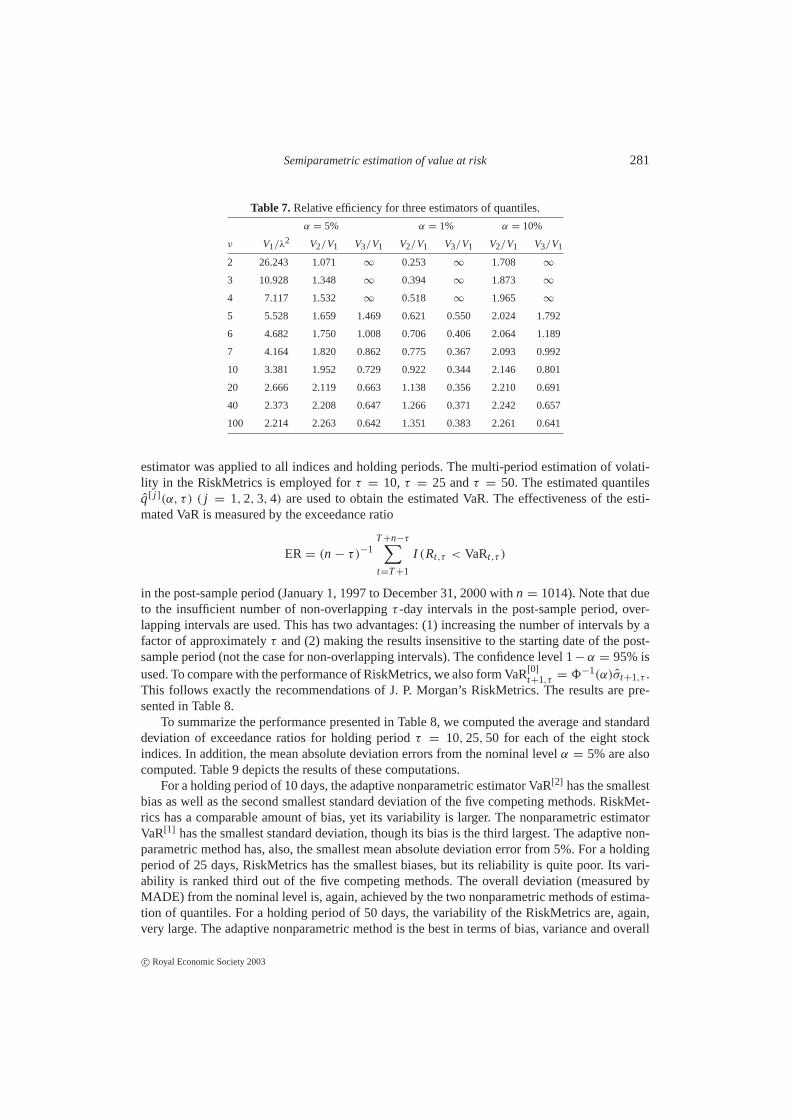
Semiparametric estimation of value at risk 281
Table 7.Relative efficiency for three estimators of quantiles.
α = 5% α = 1% α = 10%
ν V1/λ2 V2/V1 V3/V1 V2/V1 V3/V1 V2/V1 V3/V1
2 26.243 1.071 ∞ 0.253 ∞ 1.708 ∞
3 10.928 1.348 ∞ 0.394 ∞ 1.873 ∞
4 7.117 1.532 ∞ 0.518 ∞ 1.965 ∞
5 5.528 1.659 1.469 0.621 0.550 2.024 1.792
6 4.682 1.750 1.008 0.706 0.406 2.064 1.189
7 4.164 1.820 0.862 0.775 0.367 2.093 0.992
10 3.381 1.952 0.729 0.922 0.344 2.146 0.801
20 2.666 2.119 0.663 1.138 0.356 2.210 0.691
40 2.373 2.208 0.647 1.266 0.371 2.242 0.657
100 2.214 2.263 0.642 1.351 0.383 2.261 0.641
estimator was applied to all indices and holding periods. The multi-period estimation of volati-lity in the RiskMetrics is employed forτ = 10, τ = 25 andτ = 50. The estimated quantilesq[ j ](α, τ ) ( j = 1, 2, 3, 4) are used to obtain the estimated VaR. The effectiveness of the esti-mated VaR is measured by the exceedance ratio
ER = (n − τ)−1T+n−τ∑t=T+1
I (Rt,τ < VaRt,τ )
in the post-sample period (January 1, 1997 to December 31, 2000 withn = 1014). Note that dueto the insufficient number of non-overlappingτ -day intervals in the post-sample period, over-lapping intervals are used. This has two advantages: (1) increasing the number of intervals by afactor of approximatelyτ and (2) making the results insensitive to the starting date of the post-sample period (not the case for non-overlapping intervals). The confidence level 1− α = 95% isused. To compare with the performance of RiskMetrics, we also form VaR[0]
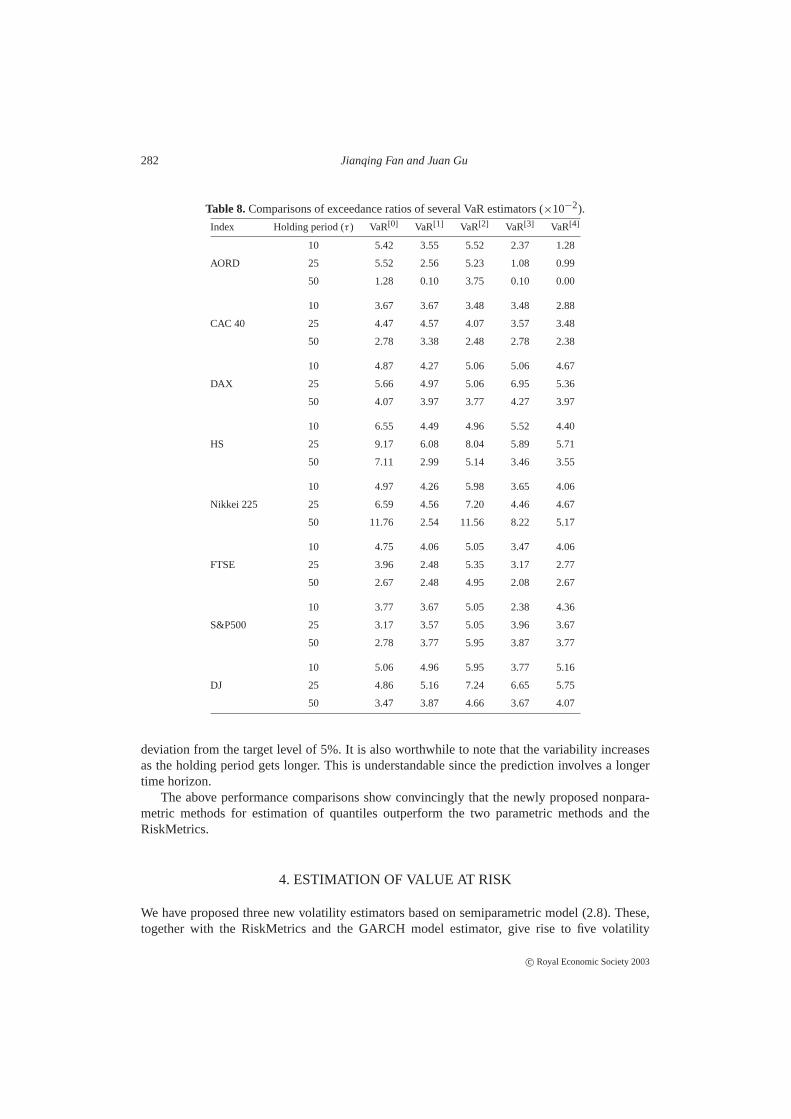
t+1,τ = 8−1(α)σt+1,τ .This follows exactly the recommendations of J. P. Morgan’s RiskMetrics. The results are pre-sented in Table 8.
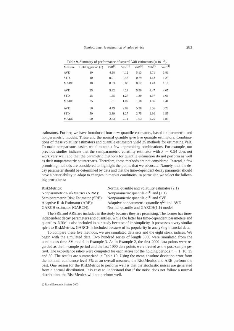
To summarize the performance presented in Table 8, we computed the average and standarddeviation of exceedance ratios for holding periodτ = 10, 25, 50 for each of the eight stockindices. In addition, the mean absolute deviation errors from the nominal levelα = 5% are alsocomputed. Table 9 depicts the results of these computations.
For a holding period of 10 days, the adaptive nonparametric estimator VaR[2] has the smallestbias as well as the second smallest standard deviation of the five competing methods. RiskMet-rics has a comparable amount of bias, yet its variability is larger. The nonparametric estimatorVaR[1] has the smallest standard deviation, though its bias is the third largest. The adaptive non-parametric method has, also, the smallest mean absolute deviation error from 5%. For a holdingperiod of 25 days, RiskMetrics has the smallest biases, but its reliability is quite poor. Its vari-ability is ranked third out of the five competing methods. The overall deviation (measured byMADE) from the nominal level is, again, achieved by the two nonparametric methods of estima-tion of quantiles. For a holding period of 50 days, the variability of the RiskMetrics are, again,very large. The adaptive nonparametric method is the best in terms of bias, variance and overall
c© Royal Economic Society 2003
282 Jianqing Fan and Juan Gu
Table 8.Comparisons of exceedance ratios of several VaR estimators (×10−2).
Index Holding period (τ ) VaR[0] VaR[1] VaR[2] VaR[3] VaR[4]
10 5.42 3.55 5.52 2.37 1.28
AORD 25 5.52 2.56 5.23 1.08 0.99
50 1.28 0.10 3.75 0.10 0.00
10 3.67 3.67 3.48 3.48 2.88
CAC 40 25 4.47 4.57 4.07 3.57 3.48
50 2.78 3.38 2.48 2.78 2.38
10 4.87 4.27 5.06 5.06 4.67
DAX 25 5.66 4.97 5.06 6.95 5.36
50 4.07 3.97 3.77 4.27 3.97
10 6.55 4.49 4.96 5.52 4.40
HS 25 9.17 6.08 8.04 5.89 5.71
50 7.11 2.99 5.14 3.46 3.55
10 4.97 4.26 5.98 3.65 4.06
Nikkei 225 25 6.59 4.56 7.20 4.46 4.67
50 11.76 2.54 11.56 8.22 5.17
10 4.75 4.06 5.05 3.47 4.06
FTSE 25 3.96 2.48 5.35 3.17 2.77
50 2.67 2.48 4.95 2.08 2.67
10 3.77 3.67 5.05 2.38 4.36
S&P500 25 3.17 3.57 5.05 3.96 3.67
50 2.78 3.77 5.95 3.87 3.77
10 5.06 4.96 5.95 3.77 5.16
DJ 25 4.86 5.16 7.24 6.65 5.75
50 3.47 3.87 4.66 3.67 4.07
deviation from the target level of 5%. It is also worthwhile to note that the variability increasesas the holding period gets longer. This is understandable since the prediction involves a longertime horizon.
The above performance comparisons show convincingly that the newly proposed nonpara-metric methods for estimation of quantiles outperform the two parametric methods and theRiskMetrics.
4. ESTIMATION OF VALUE AT RISK
We have proposed three new volatility estimators based on semiparametric model (2.8). These,together with the RiskMetrics and the GARCH model estimator, give rise to five volatility
c© Royal Economic Society 2003
Semiparametric estimation of value at risk 283
Table 9.Summary of performance of several VaR estimators (×10−2).
Measure Holding period (τ ) VaR[0] VaR[1] VaR[2] VaR[3] VaR[4]
AVE 10 4.88 4.12 5.13 3.71 3.86
STD 10 0.91 0.48 0.79 1.12 1.23
MADE 10 0.63 0.88 0.52 1.43 1.18
AVE 25 5.42 4.24 5.90 4.47 4.05
STD 25 1.85 1.27 1.39 1.97 1.66
MADE 25 1.31 1.07 1.18 1.66 1.41
AVE 50 4.49 2.89 5.28 3.56 3.20
STD 50 3.39 1.27 2.75 2.30 1.55
MADE 50 2.73 2.11 1.63 2.25 1.85
estimators. Further, we have introduced four new quantile estimators, based on parametric andnonparametric models. These and the normal quantile give five quantile estimators. Combina-tions of these volatility estimators and quantile estimators yield 25 methods for estimating VaR.To make comparisons easier, we eliminate a few unpromising combinations. For example, ourprevious studies indicate that the semiparametric volatility estimator withλ = 0.94 does notwork very well and that the parametric methods for quantile estimation do not perform as wellas their nonparametric counterparts. Therefore, these methods are not considered. Instead, a fewpromising methods are considered to highlight the points that we advocate. Namely, that the de-cay parameter should be determined by data and that the time-dependent decay parameter shouldhave a better ability to adapt to changes in market conditions. In particular, we select the follow-ing procedures:
RiskMetrics: Normal quantile and volatility estimator (2.1)Nonparametric RiskMetrics (NRM): Nonparametric quantileq[1] and (2.1)Semiparametric Risk Estimator (SRE): Nonparametric quantileq[1] and SVEAdaptive Risk Estimator (ARE): Adaptive nonparametric quantileq[2] and AVEGARCH estimator (GARCH): Normal quantile and GARCH(1,1) model.
The SRE and ARE are included in the study because they are promising. The former has time-independent decay parameters and quantiles, while the latter has time-dependent parameters andquantiles. NRM is also included in our study because of its simplicity. It possesses a very similarspirit to RiskMetrics. GARCH is included because of its popularity in analyzing financial data.
To compare these five methods, we use simulated data sets and the eight stock indices. Webegin with the simulated data. Two hundred series of length 3000 were simulated from thecontinuous-time SV model in Example 3. As in Example 2, the first 2000 data points were re-garded as the in-sample period and the last 1000 data points were treated as the post-sample pe-riod. The exceedance ratios were computed for each series for the holding periodsτ = 1, 10, 25and 50. The results are summarized in Table 10. Using the mean absolute deviation error fromthe nominal confidence level 5% as an overall measure, the RiskMetrics and ARE perform thebest. One reason for the RiskMetrics to perform well is that the stochastic noises are generatedfrom a normal distribution. It is easy to understand that if the noise does not follow a normaldistribution, the RiskMetrics will not perform well.
c© Royal Economic Society 2003

284 Jianqing Fan and Juan Gu
Table 10.Summary of the performance of five VaR estimators.
Measure Holding period (τ ) RiskMetrics NRM SRE ARE GARCH
AVE 1 5.45 4.95 4.99 4.99 4.29
STD 1 0.55 0.58 0.66 0.62 2.16
MADEa 1 0.61 0.47 0.54 0.49 1.81
AVE 10 5.19 5.12 5.16 5.12 4.29
STD 10 1.60 1.82 1.83 1.75 2.52
MADE 10 1.24 1.45 1.41 1.37 2.12
AVE 25 5.00 5.18 5.18 5.18 4.17
STD 25 2.53 2.76 2.80 2.71 3.16
MADE 25 1.96 2.14 2.16 2.04 2.73
AVE 50 5.41 5.41 5.37 5.33 4.21
STD 50 3.89 3.89 3.94 3.77 3.70
MADE 50 3.07 3.07 3.10 2.98 3.16
aMean absolute deviation error from the nominal confidence level 5%.
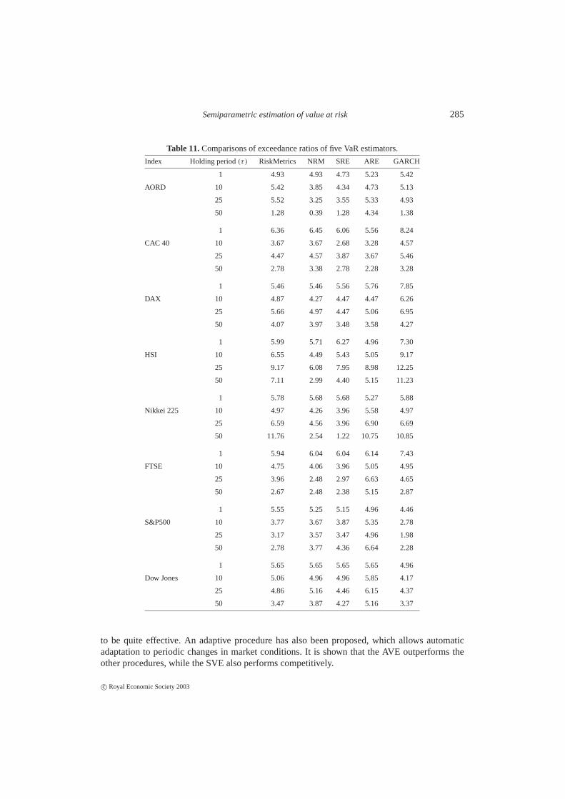
We now apply the five VaR estimators to the eight stock indices depicted in Example 1. Asin Example 1 and shown in Table 2, the post-sample was from January 1, 1997 to December 31,2000. The exceedance ratios are computed for each method. The results are shown in Table 11.To make the comparison easier, Table 12 shows the summary statistics of Table 11.
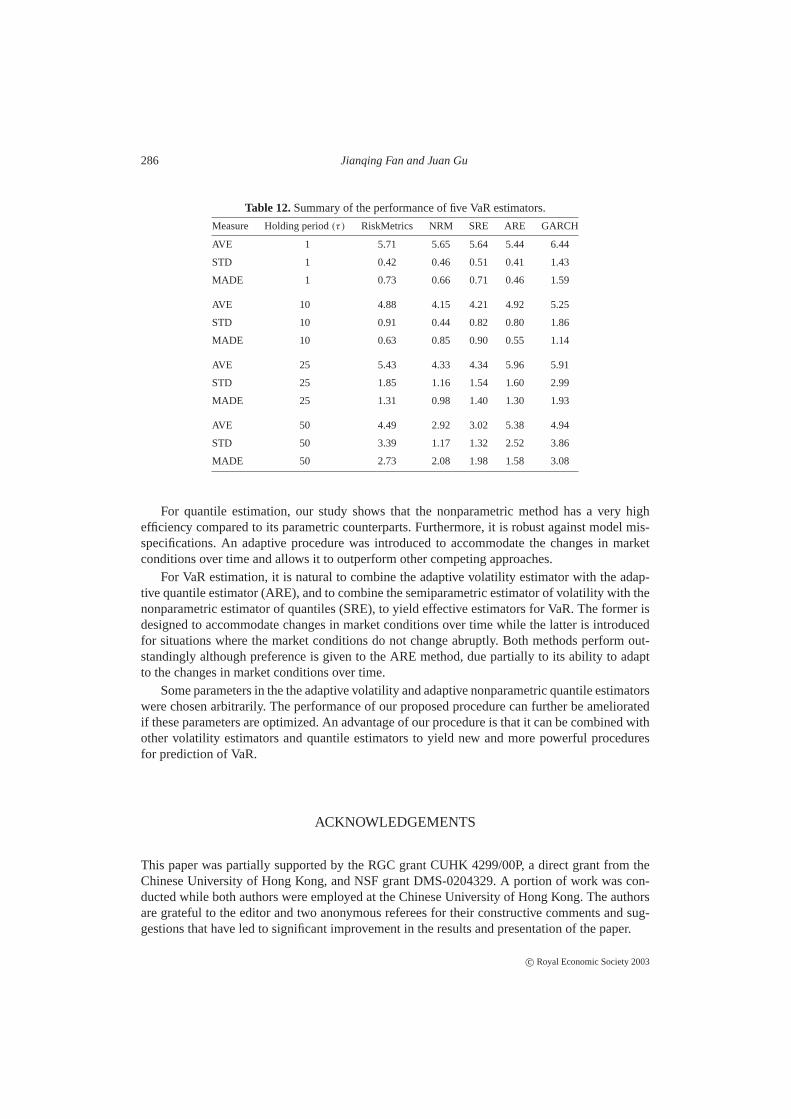
Table 12 shows that the ARE is the best procedure among the five VaR estimators for allholding periods. For one-period, SRE outperforms RiskMetrics, but for multi-period, RiskMet-rics outperforms the SRE. NRM improves somewhat the performance of RiskMetrics. For thereal data sets, it is clear that it is worthwhile to use the time-dependent methods such as ARE.Indeed, the gain is more than the price that we have to pay for the adaptation to the changes ofmarket conditions. The results also provide stark evidence that the quantile of standardized returnshould be estimated and the decay parameters should be determined from data.
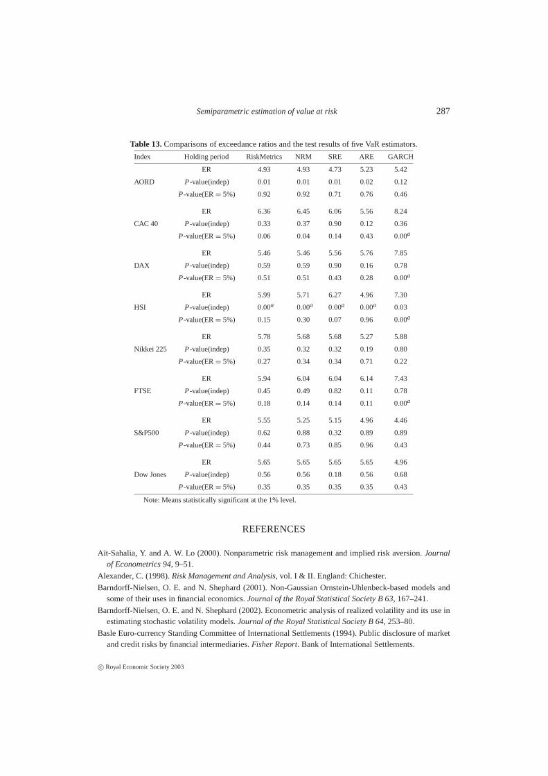
Table 13 shows the results for hypothesis testing, as in the performance measures 4 and 5.The results are shown for a 1-day holding period. As indicated before, for multiple-day VaRprediction, overlapping intervals are used. Hence, hypothesis testing cannot be applied. Exceptfor the HSI, there is little evidence against the hypothesis of independence and the hypothesisthat ER = 5%. TheP-values for AORD also tend to be small.
5. CONCLUSIONS
We have proposed semiparametric methods for estimating volatility, as well as nonparametricand parametric methods for estimating the quantiles of scaled residuals. The performance com-parisons are studied both empirically and theoretically. We have shown that the proposed semi-parametric model is flexible in approximating stock price dynamics.
For volatility estimation, it is evident from our study that the decay parameter should bechosen from data. Our proposed method of choosing the decay parameter has been demonstrated
c© Royal Economic Society 2003
Semiparametric estimation of value at risk 285
Table 11.Comparisons of exceedance ratios of five VaR estimators.
Index Holding period(τ ) RiskMetrics NRM SRE ARE GARCH
1 4.93 4.93 4.73 5.23 5.42
AORD 10 5.42 3.85 4.34 4.73 5.13
25 5.52 3.25 3.55 5.33 4.93
50 1.28 0.39 1.28 4.34 1.38
1 6.36 6.45 6.06 5.56 8.24
CAC 40 10 3.67 3.67 2.68 3.28 4.57
25 4.47 4.57 3.87 3.67 5.46
50 2.78 3.38 2.78 2.28 3.28
1 5.46 5.46 5.56 5.76 7.85
DAX 10 4.87 4.27 4.47 4.47 6.26
25 5.66 4.97 4.47 5.06 6.95
50 4.07 3.97 3.48 3.58 4.27
1 5.99 5.71 6.27 4.96 7.30
HSI 10 6.55 4.49 5.43 5.05 9.17
25 9.17 6.08 7.95 8.98 12.25
50 7.11 2.99 4.40 5.15 11.23
1 5.78 5.68 5.68 5.27 5.88
Nikkei 225 10 4.97 4.26 3.96 5.58 4.97
25 6.59 4.56 3.96 6.90 6.69
50 11.76 2.54 1.22 10.75 10.85
1 5.94 6.04 6.04 6.14 7.43
FTSE 10 4.75 4.06 3.96 5.05 4.95
25 3.96 2.48 2.97 6.63 4.65
50 2.67 2.48 2.38 5.15 2.87
1 5.55 5.25 5.15 4.96 4.46
S&P500 10 3.77 3.67 3.87 5.35 2.78
25 3.17 3.57 3.47 4.96 1.98
50 2.78 3.77 4.36 6.64 2.28
1 5.65 5.65 5.65 5.65 4.96
Dow Jones 10 5.06 4.96 4.96 5.85 4.17
25 4.86 5.16 4.46 6.15 4.37
50 3.47 3.87 4.27 5.16 3.37
to be quite effective. An adaptive procedure has also been proposed, which allows automaticadaptation to periodic changes in market conditions. It is shown that the AVE outperforms theother procedures, while the SVE also performs competitively.
c© Royal Economic Society 2003
286 Jianqing Fan and Juan Gu
Table 12.Summary of the performance of five VaR estimators.
Measure Holding period(τ ) RiskMetrics NRM SRE ARE GARCH
AVE 1 5.71 5.65 5.64 5.44 6.44
STD 1 0.42 0.46 0.51 0.41 1.43
MADE 1 0.73 0.66 0.71 0.46 1.59
AVE 10 4.88 4.15 4.21 4.92 5.25
STD 10 0.91 0.44 0.82 0.80 1.86
MADE 10 0.63 0.85 0.90 0.55 1.14
AVE 25 5.43 4.33 4.34 5.96 5.91
STD 25 1.85 1.16 1.54 1.60 2.99
MADE 25 1.31 0.98 1.40 1.30 1.93
AVE 50 4.49 2.92 3.02 5.38 4.94
STD 50 3.39 1.17 1.32 2.52 3.86
MADE 50 2.73 2.08 1.98 1.58 3.08
For quantile estimation, our study shows that the nonparametric method has a very highefficiency compared to its parametric counterparts. Furthermore, it is robust against model mis-specifications. An adaptive procedure was introduced to accommodate the changes in marketconditions over time and allows it to outperform other competing approaches.
For VaR estimation, it is natural to combine the adaptive volatility estimator with the adap-tive quantile estimator (ARE), and to combine the semiparametric estimator of volatility with thenonparametric estimator of quantiles (SRE), to yield effective estimators for VaR. The former isdesigned to accommodate changes in market conditions over time while the latter is introducedfor situations where the market conditions do not change abruptly. Both methods perform out-standingly although preference is given to the ARE method, due partially to its ability to adaptto the changes in market conditions over time.
Some parameters in the the adaptive volatility and adaptive nonparametric quantile estimatorswere chosen arbitrarily. The performance of our proposed procedure can further be amelioratedif these parameters are optimized. An advantage of our procedure is that it can be combined withother volatility estimators and quantile estimators to yield new and more powerful proceduresfor prediction of VaR.
ACKNOWLEDGEMENTS
This paper was partially supported by the RGC grant CUHK 4299/00P, a direct grant from theChinese University of Hong Kong, and NSF grant DMS-0204329. A portion of work was con-ducted while both authors were employed at the Chinese University of Hong Kong. The authorsare grateful to the editor and two anonymous referees for their constructive comments and sug-gestions that have led to significant improvement in the results and presentation of the paper.
c© Royal Economic Society 2003
Semiparametric estimation of value at risk 287
Table 13.Comparisons of exceedance ratios and the test results of five VaR estimators.
Index Holding period RiskMetrics NRM SRE ARE GARCH
ER 4.93 4.93 4.73 5.23 5.42
AORD P-value(indep) 0.01 0.01 0.01 0.02 0.12
P-value(ER= 5%) 0.92 0.92 0.71 0.76 0.46
ER 6.36 6.45 6.06 5.56 8.24
CAC 40 P-value(indep) 0.33 0.37 0.90 0.12 0.36
P-value(ER= 5%) 0.06 0.04 0.14 0.43 0.00a
ER 5.46 5.46 5.56 5.76 7.85
DAX P-value(indep) 0.59 0.59 0.90 0.16 0.78
P-value(ER= 5%) 0.51 0.51 0.43 0.28 0.00a
ER 5.99 5.71 6.27 4.96 7.30
HSI P-value(indep) 0.00a 0.00a 0.00a 0.00a 0.03
P-value(ER= 5%) 0.15 0.30 0.07 0.96 0.00a
ER 5.78 5.68 5.68 5.27 5.88
Nikkei 225 P-value(indep) 0.35 0.32 0.32 0.19 0.80
P-value(ER= 5%) 0.27 0.34 0.34 0.71 0.22
ER 5.94 6.04 6.04 6.14 7.43
FTSE P-value(indep) 0.45 0.49 0.82 0.11 0.78
P-value(ER= 5%) 0.18 0.14 0.14 0.11 0.00a
ER 5.55 5.25 5.15 4.96 4.46
S&P500 P-value(indep) 0.62 0.88 0.32 0.89 0.89
P-value(ER= 5%) 0.44 0.73 0.85 0.96 0.43
ER 5.65 5.65 5.65 5.65 4.96
Dow Jones P-value(indep) 0.56 0.56 0.18 0.56 0.68
P-value(ER= 5%) 0.35 0.35 0.35 0.35 0.43
Note: Means statistically significant at the 1% level.
REFERENCES
Aıt-Sahalia, Y. and A. W. Lo (2000). Nonparametric risk management and implied risk aversion.Journalof Econometrics 94, 9–51.
Alexander, C. (1998).Risk Management and Analysis,vol. I & II. England: Chichester.
Barndorff-Nielsen, O. E. and N. Shephard (2001). Non-Gaussian Ornstein-Uhlenbeck-based models andsome of their uses in financial economics.Journal of the Royal Statistical Society B 63, 167–241.
Barndorff-Nielsen, O. E. and N. Shephard (2002). Econometric analysis of realized volatility and its use inestimating stochastic volatility models.Journal of the Royal Statistical Society B 64, 253–80.
Basle Euro-currency Standing Committee of International Settlements (1994). Public disclosure of marketand credit risks by financial intermediaries.Fisher Report. Bank of International Settlements.
c© Royal Economic Society 2003
288 Jianqing Fan and Juan Gu
Beder, T. S. (1995). VaR: seductive but dangerous.Financial Analysts Journal 51, 12–24.Beltratti, A. and C. Morana (1999). Computing value-at-risk with high frequency data.Journal of Empirical
Finance 6, 431–55.Black, F., E. Derman and E. Toy (1990). A one-factor model of interest rates and its application to treasury
bond options.Financial Analysts Journal 46, 33–9.Black, F. and P. Karasinski (1991). Bond and option pricing when short rates are lognormal.Financial
Analysts Journal 47, 52–9.Bollerslev, T. (1986). Generalized autoregressive conditional heteroscedasticity.Journal of Econometrics
31, 307–27.Bollerslev, T. and J. Wooldridge (1992). Quasi-maximum likelihood estimation and inference in dynamic
models with time varying covariances.Econometric Reviews 11, 143–72.Chan, K. C., A. G. Karolyi, F. A. Longstaff and A. B. Sanders (1992). An empirical comparison of alterna-
tive models of the short-term interest rate.Journal of Finance 47, 1209–27.Chapman, D. A. and N. D. Pearson (2000). Is the short rate drift actually nonlinear?Journal of Finance 55,
355–88.Christoffersen, P. F. (1998). Evaluating interval forecasts.International Economic Review 39, 841–62.Cox, J. C., J. E. Ingersoll and S. A. Ross (1985). A theory of the term structure of interest rates.Economet-
rica 53, 385–467.Danielsson, J. and C. G. de Vries (2000).Value-at-Risk and Extreme Returns. London School of Economics
and Institute of Economic Studies, University of Iceland.Dave, R. D. and G. Stahl (1997). On the accuracy of VaR estimates based on the Variance–Covariance
approach, Working paper, Olshen & Associates.Diebold, F. X., A. Hickman, A. Inoue and T. Schuermann (1998). Converting 1-day volatility to h-day
volatility: scaling by√
h is worse than you think.Risk 11, 104–7.Dowd, K. (1998).Beyond value at risk: The New Science of Risk Management. New York: Wiley.Duffie, D. and J. Pan (1997). An overview of value at risk.The Journal of Derivatives 5, 7–49.Embrechts, P., C. Kluppelberg and T. Mikosch (1997).Modelling Extremal Events for Insurance and Fi-
nance. Berlin: Springer.Engle, R. F. (1995).ARCH, Selected Readings. Oxford: Oxford University Press.Engle, R. F. and G. Gonzalez-Rivera (1991). Semiparametric Arch Models.Journal of Business and Eco-
nomic Statistics 9, 345–59.Engle, R. F. and S. Manganelli (2000). CAViaR: conditional autoregressive value at risk by regression
quantile. Econom. Soc. World Cong. 2000 Contrib. paper 0841, Econometric Society.Fan, J. and I. Gijbels (1996).Local Polynomial Modelling and its Applications. London: Chapman and Hall.Fan, J., J. Jiang, C. Zhang and Z. Zhou (2003). Time-dependent diffusion models for term structure dynam-
ics and the stock price volatility.Statistica Sinica, to appear.Fan, J. and Q. Yao (2003).Nonlinear Time Series Modelling and Prediction. New York: Springer.Fan, J. and C. Zhang (2003). A reexamination of diffusion estimators with applications to financial model
validation.Journal of the American Statistical Association 98, 118–34.Genon-Catalot, V., T. Jeantheau and C. Laredo (1999). Parameter estimation for discretely observed
stochastic volatility models.Bernoulli 5, 855–72.Hardle, W., H. Herwatz and V. Spokoiny (2003). Time inhomogeneous multiple volatility modelling.
Financial Econometrics, to appear.Hendricks, D. (1996). Evaluation of value-at-risk models using historical data.Federal Reserve Bank of
New York Economic Policy Review, 39–69.Hull, J. and A. White (1990). Pricing interest rate derivative securities.Review of Financial Studies 3,
573–92.
c© Royal Economic Society 2003
Semiparametric estimation of value at risk 289
Jackson, P., D. J. Maude and W. Perraudin (1997). Bank capital and value-at-risk.Journal of Derivatives,73–111.
Jorion, P. (2000).Value at Risk: The New Benchmark for Managing Financial Risk, 2nd edn. New York:McGraw-Hill.
Lucas, A. (2000). A note on optimal estimation from a risk-management perspective under possible mis-specified tail behavior.Journal of Business and Economic Statistics 18, 31–9.
Mahoney, J. M. (1996). Forecast biases in value-at-risk estimations: evidence from foreign exchange andglobal equity portfolios, Working paper, Federal Reserve Bank of New York.
Mercurio, D. and V. Spokoiny (2003). Statistical inference for time-inhomogeneous volatility models.TheAnnals of Statistics(forthcoming).
Morgan, J. P. (1996).RiskMetrics Technical Document, 4th edn. New York.Pant, V. and W. Chang (2001). An empirical comparison of methods for incorporating fat tails into VaR
models.Journal of Risk 3, 1–21.Prakasa Rao, B. L. S. (1987).Asymptotic Theory of Statistical Inference. New York: John Wiley & Sons.Stanton, R. (1997). A nonparametric models of term structure dynamics and the market price of interest
rate risk.Journal of Finance LII, 1973–2002.Wong, C.-M. and M. K. P. So (2003). On conditional moments of GARCH models, with applications to
multiple period value.Statistica Sinica(forthcoming).Yang, L. J., W. Hardle and J. P. Nielsen (1999). Nonparametric autoregression with multiplicative volatility
and additive mean.Journal of Time Series Analysis 20, 579–604.Yatchew, A. and W. Hardle (2003). Dynamic nonparametric state price density estimation using constrained
least-squares and the bootstrap.Journal of Econometrics(forthcoming).
APPENDIX
In this Appendix, we give some theoretical derivations on the relative efficiencies of severalnonparametric and parametric estimators of quantiles. The basic assumption is that{εt,τ , t =
T0, . . . , T − τ } is an independent random sample from a population with probability densityf .
A.1. Relative efficiency of estimator (3.1)
By the symmetry assumption,f (q(α, τ )) = f (q(1−α, τ)). By using (3.8), we obtain that the es-timatorsq(α, τ ) andq(1−α, τ) are joint asymptotically normal with mean(q(α, τ ),−q(α, τ ))T
and covariance matrix
f (q(α, τ ))−2(
α(1 − α) α2
α2 α(1 − α)
).
It follows thatq[3](α, τ ) has the asymptotic normal distribution with meanq(α, τ ) and variance
4−1 f (q(α, τ ))−2[α(1 − α) − 2α2
+ α(1 − α)] = 2−1 f (q(α, τ ))−2α(1 − 2α),
and thatq(α, τ ) is asymptotically normal with meanq(α, τ ) and variance
f (q(α, τ ))−2α(1 − α).
Consequently, the estimatorq[3](α, τ ) is a factor of 2(1 − α)/(1 − 2α) as efficient asq(α, τ ).
c© Royal Economic Society 2003

290 Jianqing Fan and Juan Gu
A.2. Asymptotic normality for the method of moments estimator
Recall that the variance of the squaredt-random variable with degree of freedomν is given by2ν2(ν − 1)/(ν − 2)2(ν − 4). By the central limit theorem,
√m
(µ2 −
ν
ν − 2λ2)
L−→ N
(0,
2ν2(ν − 1)
(ν − 2)2(ν − 4)λ4
).
Using the delta method, we deduce that
√m
(√µ2 −
√ν
ν − 2λ
)L
−→ N
(0,
ν(ν − 1)
2(ν − 2)(ν − 4)λ2)
.
Hence, the estimated quantile
q[4](α, τ ) =
õ2
√ν − 2
νt (α, τ )
has the asymptotic normal distribution with meanλt (α, τ ) and variance
λ(ν − 1)t (α, τ )2
2(ν − 4).
c© Royal Economic Society 2003