seminar- robust regression methods
TRANSCRIPT
ROBUST REGRESSION METHOD
Seminar Report submitted toThe National Institute of Technology, Calicut
for the award of the degree
of
Master of Mathematics
by
Sumon Jose
under the guidance of
Dr. Jessy John C.
Department of Mathematics
NIT, CalicutDecember 2014
c© 2014, SumonJose. All rights reserved.

to all my teachers
who made me who I am

DECLARATION
I, hereby declare that the seminar report entitled ”ROBUST REGRESSION METHOD” is
the report of the seminar presenation work carried out by me, under the supervision and
guidance of Dr. Jessy John C., Professor, Department of Mathematics, National Institute
of Technology Calicut, in partial fulfillment of the requirements for the award of degree of
M.Sc. Mathematics and this seminar report has not previously formed the basis of any
degree, diploma, fellowship or other similar titles of universities or institutions.
Signature:
SUMON JOSE
Place: Calicut
Date:08/12/2014

CERTIFICATE
I hereby certify that this seminar report entitled ”ROBUST REGRESSION METHOD” is
a bona fide record of the seminar, carried out by Mr. Sumon Jose in partial fulfillment of
the requirements for the degree of M.Sc. Mathematics at National Insitute of Technology,
Calicut, during the thrid semester(Monsoon Semester, 2014-15).
Dr. Jessy John C
Professor, Dept. of Mathematics, NITC

Acknowledgement
As I present this work of mine, my mind wells up with gratitude to several people who
have been instrumental in the successful completion of this seminar work. May I gratefully
remember all those who supported me through their personal interest and caring assistance.
At the very outset it is with immense pleasure that I place on record the immense gratitutde
I hold to my erudite guide Dr. Jessy John C, Department of Mathematics, National Insti-
tute of Technology, Calicut, for her inspiring guidance, invaluably constructive criticism and
friendly advice during the prepration for this seminar. I propose my sincere thanks to Dr.
Sanjay P K, Co-ordinator and Faculty Advisor, who in his unassuming ways have helped me
and guided me in this endevor. I express my sincere thanks to Mr. Yasser K T, Mr. Aswin,
Ms. Ayisha Hadya, Ms. Pavithra Celeste and many others who helped me a lot in different
ways in completing this presentation successfully.
Sumon Jose

Abstract
Regression is a statistical tool that is widely employed in forecasting and prediction andtherefore a very fast growing branch of Statistics. The classical Linear Regression Modelconstructed by the ordinary least square method is the best method whenever the basicassumptions of the model are met with. However this model has a draw back when the datacontain outliers. The Robust regression method is developed in handling such situations andhence it plays a vital role in regression studies.
In the first seminar the concepts of Outliers and Leverage points were introduced. Throughdata analysis it was showed that the presence of outliers or leverage points could contami-nate our estimation process. Analytical proof was given to the fact that heavier tailed nonnormal error distribution does not result in the ordinary least square method. However asall the outliers are not erroneous data, instead could be sample peculiarities or they musthave come about due to certain factors that are not considered in the study.
Now, in the second seminar the task is to lay out the desirable properties, strengths andweaknesses that Robust Regression Estimator should have in order to reach a better esti-mate. To achieve this aim, a brief account of the concepts of robustness and resistance isincluded in this second seminar. Another point that deserves attention is the concept ofFinite Sample Break Down Point(BDP). The notion of BDP is defined and a mathematicalexpression is given for the same.
The main idea that is handled in this presentation is the idea of M-estimators. The ini-tial task is to make a scale equivariant M estimator in a generic manner and thereafter thekey ideas of weight function and influence function are handled. Graphical explanations ofthe concept of re-descending estimators are given and they are applied for the regressionpurpose. To give a sure footing to the ideas handled, a demonstration of the same is donethrough a problem that analyses a delivery time issue affected by two variables. The errorfactor in the problem demonstrates the betterment in the solution as various M-estimatorsof Huber, Ramasay, Andrew and Hampell are employed for the estimation purpose. Finallya concluding analysis of the problem is given and I have also done a quick survey of otherRobust Regression Methods. However a detailed study of all the M estimators are avoidedas currently they are replaced by a better version, MM estimators which provide a muchbetter estimate. It is proposed to that a detailed study of the latter be undertaken duringthe final project work.

Contents
Dedication 2
Declaration 3
Certificate by the Supervisor 4
Acknowledgement 5
Abstract 6
Contents 7
1 Preliminary Notions 1
1.1 Introduction . . . . . . . . . . . . . . . . . . . . . . . . . . . . . . . . . . . . 1
1.2 The Classical Method . . . . . . . . . . . . . . . . . . . . . . . . . . . . . . . 1
1.3 Basic Definitons . . . . . . . . . . . . . . . . . . . . . . . . . . . . . . . . . . 2
1.3.1 Residuals . . . . . . . . . . . . . . . . . . . . . . . . . . . . . . . . . 2
1.3.2 Outliers . . . . . . . . . . . . . . . . . . . . . . . . . . . . . . . . . . 3
1.3.3 Leverage . . . . . . . . . . . . . . . . . . . . . . . . . . . . . . . . . . 4
1.3.4 Influence . . . . . . . . . . . . . . . . . . . . . . . . . . . . . . . . . . 5
1.3.5 Rejection Point . . . . . . . . . . . . . . . . . . . . . . . . . . . . . . 6
1.4 The Need for Robust Regression . . . . . . . . . . . . . . . . . . . . . . . . . 6
1.5 Avantages of the Robust Regression Procedure . . . . . . . . . . . . . . . . . 6
1.6 Desirable Properties . . . . . . . . . . . . . . . . . . . . . . . . . . . . . . . 6
1.6.1 Qualitative Robustness . . . . . . . . . . . . . . . . . . . . . . . . . . 7
1.6.2 Infenitesimal Robustness . . . . . . . . . . . . . . . . . . . . . . . . . 7
1.6.3 Quantitative Robustness . . . . . . . . . . . . . . . . . . . . . . . . . 7
1.7 Conclusion . . . . . . . . . . . . . . . . . . . . . . . . . . . . . . . . . . . . . 7
2 ROBUST REGRESSION ESTIMATORS: M-ESTIMATORS 8
2.1 Introduction . . . . . . . . . . . . . . . . . . . . . . . . . . . . . . . . . . . . 8
2.2 Approach . . . . . . . . . . . . . . . . . . . . . . . . . . . . . . . . . . . . . 8
2.3 Strengths and Weaknesses . . . . . . . . . . . . . . . . . . . . . . . . . . . . 9
2.3.1 Finite Sample Breakdown Point . . . . . . . . . . . . . . . . . . . . . 9
7
2.3.2 Relative Efficiency . . . . . . . . . . . . . . . . . . . . . . . . . . . . 9
2.4 M- Estimators . . . . . . . . . . . . . . . . . . . . . . . . . . . . . . . . . . . 10
2.4.1 Constructing a Scale Equivariant Estimator . . . . . . . . . . . . . . 11
2.4.2 Finding an M-Estimator . . . . . . . . . . . . . . . . . . . . . . . . . 12
2.4.3 Re- Descending Estimators . . . . . . . . . . . . . . . . . . . . . . . . 13
2.4.4 Robust Criterion Functions . . . . . . . . . . . . . . . . . . . . . . . 15
2.5 Properties of M-Estimators . . . . . . . . . . . . . . . . . . . . . . . . . . . . 20
2.5.1 BDP . . . . . . . . . . . . . . . . . . . . . . . . . . . . . . . . . . . . 20
2.5.2 Efficiency . . . . . . . . . . . . . . . . . . . . . . . . . . . . . . . . . 20
2.6 Conclusion . . . . . . . . . . . . . . . . . . . . . . . . . . . . . . . . . . . . . 20
Conclusions and Future Scope 21
References 22
8

Chapter 1
Preliminary Notions
1.1 Introduction
Regression analysis is a powerful statistical tool used to establish and investigate the re-
lationship between variables. Here the purpose is to ascertain the effect of one or more
variable/variables on another variable. For example the effect of price hike of petroleum
products on the cost of vegetables. Very evidently there exists a linear relationship between
these two variables. And therefore Regression techniques have been the very basis of eco-
nomic statistics. But later studies found that the classical ordinary least square method
which was usually employed in this area had its weaknesses as it is very vulnerable whenever
there are outliers present in the data. This chapter aims at giving a birds eye view of the
classical Least Square Estimation method (which gives the maximum likelihood estimate in
the well behaved case), developing the various basic definitons that are needed to understand
the notion of Robust Regression and establishes the weaknesses of the ordinary least square
method.
1.2 The Classical Method
The classical linear regression model relates the dependednt or response variables yi to in-
dependent explanatory variables xi1, xi2, ..., xip for i = 1, .., n, such that
yi = xTi β + εi, (1.1)
for i=1,...,n where xTi = (xi1, xi2, ..., xip), εi denote the error terms and β = (β1, β2, ..., βp)T
The expected value of yi called the fitted value is
yi = xTi β (1.2)
1

Chapter 1. Preliminary Notions 2
and one can use this to calculate the residual for the ith case,
ri = yi − yi (1.3)
In the case of simple linear regression model, we may calculate the value of β0 and β1 using
the following formulae:
β1 =
∑ni=1 yixi −
∑ni=1 yi
∑ni=1 xi
n∑ni=1 x
2i −
(∑ni=1 xi)
2
n
(1.4)
β0 = y − β1x (1.5)
The vector of fitted values yi curresponding to the observed value yi may be expressed as
follows:
y = Xβ (1.6)
1.3 Basic Definitons
1.3.1 Residuals
Definition 1.1 The difference between the observed value and the predicted value based on
the regression equation is know as the residual or error arising from a regression fit.
Mathematically the ith resudual may be expressed as ei = yi − yi where ei is the residual or
error, yi is the ith observed value and yi is the predicted value.
Suppose we use the ordinary least square method to calculate the effect of the independent
variables on the dependent variable, we can express the above formula as follows:
ei = yi − yi = yi − (β0 + β1Xi) (1.7)
where β0 and β1 are the matrices representing the paramenteres and Xi dentotes the matrix
of the values of the independent variables. The analysis of residuals play an important role
in the regression techniques as they tell us how much the observed value varies from the
predicted value. The residuals are important factors in determining the adaquecy of the fit
and in detecting the departures from the underlying assumptions of the model.

Chapter 1. Preliminary Notions 3
Example 1.1 A Panel of two judges, say P and Q graded seven perfomances of a reality
show by independently awarding marks as follows:
Judge A 40 38 36 35 39 37 41Judge B 46 42 44 40 43 41 45
A Simple least square regression fit would give the regression line as y = .75x+ 5.75 and
accordingly we will get the predicted values and error values as shown in the following table.
No. xi yi y = .75x+ 5.75 ei1 46 40 40.25 -.252 42 38 37.25 .753 44 36 38.75 -2.754 40 35 35.75 -.755 43 39 38 16 41 37 36.5 .57 45 41 39.5 1.5
1.3.2 Outliers
Definition 1.2 An outlier among the residuals is one that is far greater than the rest in
absolute value. An outlier is a peculiarity and indicates a data point that is not typical of
the rest of the data.
An outlier is an observation with a large residual value. As the definition indicates an outlier
is an observation whose dependent variable value is unusual. Outliers are of major concern
in regression analysis as they may seriously disturb the fitness of the classical ordinary least
square method.
An outlier may arise due to a sample peculiarity, errors in the data entry or due to rounding
off errors. However all outliers need not be erroneous data, instead they could be due to
certain exceptional occurances. It can also be that some of the outliers could be the result
of some factors not considered in the given study. So in general unusual observations are not
all bad observations. So deleting them is not a choice for the analyst and moreover in large
data it is often difficult to spot the outlying data.
Example 1.2 The following data gives a good demonstration of the impact of an outlier on
the least square regression fit.

Chapter 1. Preliminary Notions 4
x 1 2 2.5 4 5 6 7 7.5y 1 5 3 7 6.5 9 11 5
While pursuing the ordinary least square method we get the regression line as y = 2.12+.971x
which has outlying data as it can be very clearly understood from the figure where as a better
fit for the same would be the regression line y = .715 + 1.45x
1.3.3 Leverage
Definition 1.3 Leverage is a meaure of how an independent variable deviates from its mean.
An observation with an extreme value on a predictor variable is a point with high leverage.
Example 1.3 Consider the following data and the curresponding scatter plot.x 1 2 3 4 5 6 7 30y -1 1 3 5 7 8.5 11.5 55
The residual plot given above indicates the presence of leverage point in the data.

Chapter 1. Preliminary Notions 5
1.3.4 Influence
Definition 1.4 An observation is said to be influential if removing that observation sub-
stantially changes the estimation of the coefficients.
A useful approach to the assessment and treatment of an outlier in a least square fit would
be to determine how well the least square relationship would fit the given data when that
point is omitted.
Consider the leniar regression model in a multivariate case. In terms of matrices it may be
expressed as follows:
y = Xβ + ε (1.8)
where Y is an n × 1 vector of observations, X is an n × p matrix of levels of the regressor
variables, β is a p× 1 vector of the regression coefficients and ε is an n× 1 vector of errors.
We wish to find out the vector of least square estimators β that minimizes
S(β) =n∑i=1
ε2i = ε′ε = (y −Xβ)
′(y −Xβ) (1.9)
Expanding, differentiating(minimizing) and equating to zero we get the normal equations as
follows:
X′Xβ = X
′y (1.10)
Thus we obtain the currespnding regression model as follows:
y = x′β (1.11)
The vector of fitted values yi curresponding to the observed value yi may be expressed as
follows:
y = Xβ = X(X′X)−1X
′y = Hy (1.12)
where the n × n matrix H is called the HAT MATRIX. H = X(X′X)−1X
′The diagonal
elements of the HAT MATRIX hii measures the impact that yi has on yi. These elements
curresponding to the points (xi, yi) will tell us how far the observation xi is from the center
of the X values. Thus we can identify the influence yi has on the value of yi.
When the influence hii is large yi is more sensitive to changes in yi than when hii is relatively
small.

Chapter 1. Preliminary Notions 6
1.3.5 Rejection Point
Definition 1.5 Rejection point is the point beyond which the influence function becomes
zero.
That is the contribution of the points beyond the rejection point to the final estimate is
comparatively neglible.
1.4 The Need for Robust Regression
The need for a robust estimator for determining the parameters arises due to the fact that
the classical regression method which is the ordinary least square method does not offer a
good fit for the data
• when the error has a non-normal heavier tailed distribution (eg. Double Exponential)
• when there are outliers present in the data
Therefore we need a method that is robust against deviations from the model assuptions. As
the very name indicates the robust estimators are those which are not influenced or affected
by outliers and leverage points.
1.5 Avantages of the Robust Regression Procedure
The robust regression estimators are designed to dampen the effect of highly influential data
on the goodness of the fit. Whereas they offer the same results as the ordinary least square
method when there are no outliers or leverage points. Another very important advantage is
that they offer a relatively simple estimation procedure. Moreover they offer an alternative
to the ordianry least square fit when the fundamental assuptions of the least square method
are unfulfilled by the nature of the data.
1.6 Desirable Properties
For effective analysis and computational simplicity it is desirable that the robust estimators
would have the properties of qualitative, infinitesimal and quantitative robustness.

Chapter 1. Preliminary Notions 7
1.6.1 Qualitative Robustness
Consider any function f(x). Suppose it is desired to impose a restriction on this function
so that it does not change drastically with small changes in x. One way of doing this is to
insist that f(x) is continuous.
For example, consider the function f(x) = 0 whenever x ≤ 1 and f(x) = 10, 000 whenever
x > 1. This function can produce drastic changes with a small shift in the value of x. In
complicated regression procedure this might cause large error and hence we need to have the
property of qualitative robustness.
Definition 1.6 The property of continuity of an estimated measure is called qualitative ro-
bustness.
1.6.2 Infenitesimal Robustness
Definition 1.7 The infenitesimal robustness property requres that the estimator is differen-
tiable and that the derivative is bounded.
The purpose of this property is to ensure that small changes in x does not create drastic
impat on f(x).
1.6.3 Quantitative Robustness
This property ensures that the quantitative effect of a variable is also minimized. For example
consider f(x) = x2 and g(x) = x3. Here evidently, f(x) has a better quantitative robustness
than g(x).
1.7 Conclusion
In conclusion, the classical ordinary least square method is not always the best of options to
perform the regression analysis. Therefore we need to have other alternative methods that
have the efficency and efficasy of the OLS and at the same time are robust to deviations
from the model.

Chapter 2
ROBUST REGRESSIONESTIMATORS: M-ESTIMATORS
2.1 Introduction
Robust Regression Estimators aim to fit a model that describes the majority of the sample.
Their robustness is achieved by giving the data different weights. Whereas in the least square
approximation method all the data points are treated equally without giving weights. This
chapter aims at giving a brief idea about the M estimators. Of course, these are not the
best of estimators in all the cases. However in the transition of knowledge, these play an
important role. Because these estimators clear the ambiguity on leverage points.
2.2 Approach
Robust estimation methods are powerful tools in the detection of outliers in complicated data
sets. But unless the data is well behaved different estimators would give different estimates.
However, on their own, they do not provide a final model. A healthy approach would be to
emply both robust regression methods as well as the least square method and to compare
the results.
8

Chapter 2. M-Estimators 9
2.3 Strengths and Weaknesses
2.3.1 Finite Sample Breakdown Point
Definition 2.1 Breakdown point is the measure of the resistance of an estimator. The BDP
(Break Down Point) of a regression estimaor is the smallest fraction of contamination that
can cause the estimator to breakdon and no longer represent the trend of the data.
When an estimator breaks down, the estimate it produces from the contaminated data can
become arbitrarily far from the estimate than it would give when the data was uncontami-
nated.
In order to describe the BDP mathematically, define T as a regression estimator, Z as a
sample of n data points and T (Z) = β. Let Z′
be the corrupted sample where m of the
original data points are replaced with arbitrary values. The maximum effect that could be
caused by such contamination is
effect(m;T, Z) = supz′ |T (Z′)− T (Z)| (2.1)
When (7) is infinite, an outlier can have an arbitrarily large effect on T . The BDP of T
at the sample Z is therefore defined as:
BDP (T, Z) = min{mn
: effect(M ;T, Z)is infinite} (2.2)
The Least Square Method estimator for example has a breakdown point of 1n
because just one
leverage point can cause it to breakdown. As the number of data increases, the breakdown
point tends to 0 and so it is said to that the least squares estimator has BDP 0%.
The highest breakdown point one can hope for is 50% as if more than half the data is
contaminated that one cannot differentiate between ’good’ and ’bad’ data.
2.3.2 Relative Efficiency
Definition 2.2 The efficiency of an estimator for a particular parameter is defined as the
ratio of its minimum possible variance to its actual variance. Strictly, an estimator is con-
sidered ’efficient’ when this ratio is one.
High efficiency is crucial for an estimator if the intention is to use an estimate from sample
data to make inference about the larger population from which the same was drawn. In

Chapter 2. M-Estimators 10
general, relative efficiency compares the efficiency of an estimator to that of a well known
method. In the context of regression, estimators are compared to the least square estimator
whch is the most efficient estiamtor known as it is also the maximum likelihood estimator
in the well behaved case.
Given two estimators T1 and T2 for a population parameter β, where T1 is the most
efficient estimator possible and T2 is less efficient, the relative efficiency of T2 is calculated
as the ratio of its mean squared error to the mean squared error of T1
Efficiency(T1, T2) =E[(T1 − β)2]
E[(T2 − β)2](2.3)
2.4 M- Estimators
The M- estimators which mark a new generation among the regression estimators were first
proposed by Huber in 1973 and were later developed by many recent statisticians. However
the early M estimators had weaknesses in terms of one or more of the desired properties.
Later on from these developed the modern means for a better analysis of regression. M-
estimation is based on the idea that while we still want a maximum likelihood estimator,
the errors might be better represented by a different heavier tailed distribution.
If the probability distribution function of the error of f(εi), then the maximum likelihood
estimator for β is that which maximizes the likelihood function
n∏i=1
f(εi) =n∏i=1
f(yi − xTi β) (2.4)
This means, it also maximizes the log-likelihood function
n∑i=1
ln f(εi) =n∑i=1
ln f(yi − xTi β) (2.5)
When the errrors are normally distributed it has been shown that this leads to minimising
the sum of squared residuals, which is the ordinary least square method.
Assuming the the errors are differently distributed, leads to the maximum likelihood
esimator, minimising a different function. Using this idea, an M-estimator β minimizes
n∑i=1
ρ(εi) =n∑i=1
ρ(yi − xTi β) (2.6)
where ρ(u) is a continuous, symmetric function called the objectve function with a unique
minimum at 0. NB:

Chapter 2. M-Estimators 11
1. Knowing the appropriate ρ(u) to use requires knowledge of how the errors are really
distributed.
2. Functions are usually chosen through consideration of how the resulting estimator
down-weights the larger residuals
3. A Robust M-estimator achieves this by minimizing the sum of a less rapidly increasing
objective function than the ρ(u) = u2 of the least squares
2.4.1 Constructing a Scale Equivariant Estimator
The M-estimators are not necessarily always scale invariant i.e. if the errors yi − xTi β were
multiplied by a constant, the new solution to the above equation might not be the same as
the scaled version of the old one.
To obtain a scale invariant version of this estimator we usually solve,
n∑i=1
ρ(εis
) =n∑i=1
ρ(yi − xTi β
s) (2.7)
A popular choice for s is the re-scaled median absolute deivation
s = 1.4826XMAD (2.8)
where MAD is the Median Absolute Deviation
MAD = Median|yi − xTi β| = Median|εi| (2.9)
’s’ is highly resistant to outlying observations, with BDP 50%, as it is based on the median
rather than the mean. The estimator rescales MAD by the factor 1.4826 so that when the
sample is large and εi really distributed as N(0, σ2)), s estimates the standard deviation.
With a large sample and εi ∼ N(0, σ2):
P (|εi| < MAD) ≈ 0.5
⇒ P (| εi−0σ| < MAD
σ) ≈ 0.5
⇒ P (|Z| < MADσ
) ≈ 0.5
⇒ MADσ≈ Φ−1(0.75)
⇒ MADΦ−1 ≈ σ
1.4826 X MAD ≈ σ
Thus the tuning constant 1.4826 makes s an approximately unbiased estimator of σ if n is
large and the error distribution is normal.

Chapter 2. M-Estimators 12
2.4.2 Finding an M-Estimator
To obtain an M-estimate we solve,
Minimizeβ
n∑i=1
ρ(εis
) = Minimizeβ
n∑i=1
ρ(yi − x
′iβ
s) (2.10)
For that we equate the first partial derivatives of ρ with respect to βj (j=0,1,2,3,...,k) to
zero, yielding a necessary condition for a minimum.
This gives a system of p = k + 1 equations
n∑i=1
Xijψ(yi − x
′iβ
s) = 0, j = 0, 1, 2, ..., k (2.11)
where ψ = ρ′ and Xij is the ith observation on the jth regressor and xi0 = 1. In general ψ is
a non-linear function and so equation (17) must be solved iteratively. The most widely used
method to find this is the method of iteratively re-weighted least squares.
To use iteratively reweighted least squares suppose that an initial estimate of β0 is available
and that s is an estimate of the scale. Then we write the p = k + 1 equations as:
n∑i=1
Xijψ(yi − x
′iβ
s) =
n∑i=1
xij{ψ[(yi − x′iβ)/s]/(yi − x′iβ)/s}(yi − x′iβ)
s= 0 (2.12)
asn∑i=1
XijW0i (yi − xiβ) = 0, j = 0, 1, 2, ..., k (2.13)
where
W 0i =
ψ[
(yi−x′iβ)
s]
(yi−x′iβ)
s
if yi 6= x′iβ0
1 if yi = x′iβ0
(2.14)
We may write the above equation in matrix form as follows:
X′W 0Xβ = X
′W 0y (2.15)
where W0 is an n X n diagonal matrix of weights with diagonal elements given by the
expression
W 0i =
ψ[
(yi−x′iβ)
s]
(yi−x′iβ)
s
if yi 6= x′iβ0
1 if yi = x′iβ0
(2.16)

Chapter 2. M-Estimators 13
From the matrix form we realize that the expression is same as that of the usual weighted
least squares normal equation. Consequently the one step estimator is
β1 = (X′W 0X)−1X
′W 0y (2.17)
At the next step we recompute the weights from the equation for W but using β1 and not
β0
NOTE:
• Usually only a few iterations are required to obtain convergence
• It could be easily be implemented by a computer programme.
2.4.3 Re- Descending Estimators
Definition 2.3 Re- descending M estimators are those which have influence functions that
are non decreasing near the origin but decreasing towards zero far from the origin.
Their ψ can be chosen to redescend smoothly to zero, so that they usually satisfy ψ(x) = 0
for all |x| > r where r is referred to as the minimum rejection point. The following are few
examples for re-descending type estimators:

Chapter 2. M-Estimators 14

Chapter 2. M-Estimators 15
2.4.4 Robust Criterion Functions
The following table gives the commonly used robust criterion functions:
Citerion ρ ψ(z) w(x) rangeLeast
Squares z2
2z 1.0 |z| <∞
Huber’s
t-function z2
2z 1.0 |z| < t
t = 2 |z|t− t2
2tsign(z) t
|z| |x| > t
Andrew’s
Wave function a(1− cos( za)) sin( z
a)
sin( za
)za
|z| ≤ aπ
To understand the Robust M-estimators better, let us consider an example:
Chapter 2. M-Estimators 16
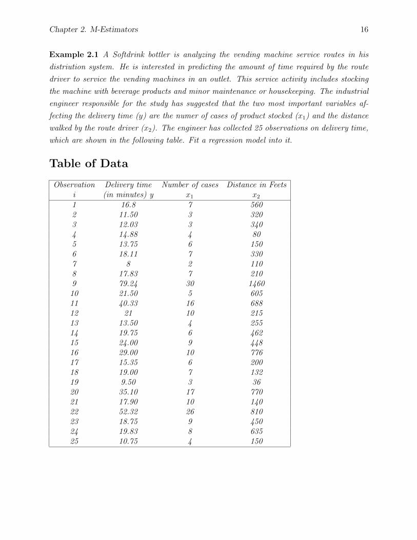
Example 2.1 A Softdrink bottler is analyzing the vending machine service routes in his
distriution system. He is interested in predicting the amount of time required by the route
driver to service the vending machines in an outlet. This service activity includes stocking
the machine with beverage products and minor maintenance or housekeeping. The industrial
engineer responsible for the study has suggested that the two most important variables af-
fecting the delivery time (y) are the numer of cases of product stocked (x1) and the distance
walked by the route driver (x2). The engineer has collected 25 observations on delivery time,
which are shown in the following table. Fit a regression model into it.
Table of Data
Observation Delivery time Number of cases Distance in Feetsi (in minutes) y x1 x2
1 16.8 7 5602 11.50 3 3203 12.03 3 3404 14.88 4 805 13.75 6 1506 18.11 7 3307 8 2 1108 17.83 7 2109 79.24 30 1460
10 21.50 5 60511 40.33 16 68812 21 10 21513 13.50 4 25514 19.75 6 46215 24.00 9 44816 29.00 10 77617 15.35 6 20018 19.00 7 13219 9.50 3 3620 35.10 17 77021 17.90 10 14022 52.32 26 81023 18.75 9 45024 19.83 8 63525 10.75 4 150

Chapter 2. M-Estimators 17
Applying the Ordinary Least Square Method we get the estimates as the following.
Least Square Fit of the Delivery Time Data
Obs. yi yi ei Weight
1 .166800E+02 .217081E+02 -.502808E+01 .100000E+012 0115000E+02 .103536E+02 .114639E+01 .100000E+013 .120300E+02 .120798E+02 -.497937E-01 .100000E+014 .148800E+02 .995565E+01 .492435E+01 .100000E+015 .137500E+02 .141944E+02 -.444398E+00 .100000E+016 .181100E+02 .183996E+02 -.289574E+00 .100000E+017 .800000E+01 .715538E+01 .844624E+00 .100000E+018 .178300E+02 .166734E+02 .115660E+02 .100000E+019 .792400E+02 .718203E+02 .741971E+01 .100000E+01
10 .215000E+02 .191236E+02 .237641E+01 .100000E+0111 .403300E+02 .380925E+02 .223749E+01 .100000E+0112 .2100000E+02 .215930E+02 -.593041E+00 .100000E+0113 .135000E+02 .124730E+02 .102701E+01 .100000E+0114 .197500E+02 .186825E+02 .106754E+01 .100000E+0115 .240000E+02 .233288E+02 .671202E+00 .100000E+0116 .290000E+02 .296629E+02 -.662928E+00 .100000E+0117 .153500E+02 .149136E+02 .436360E+00 .100000E+0118 .190000E+02 .155514E+02 .344862E+01 .100000E+0119 .950000E+01 .770681E+01 .179319E+01 .100000E+0120 .351000E+02 .408880E+02 -.578797E+01 .100000E+0121 .179000E+02 .205142E+02 -.261418E+01 .100000E+0122 .523200E+02 .560065E+02 -.368653E+01 .100000E+0123 .187500E+02 .233576E+02 -.460757E+01 .100000E+0124 .198300E+02 .244029E+02 -.457285E+01 .100000E+0125 .107500E+02 .109626E+02 -.212584E+00 .100000E+01
One important point to be noted here is that the ordinary least square method weighs all
the data points equally. All the points are given the weight as one as it can be seen from the
last column. Accordingly we have the following values for the parameters:
β0 = 2.3412
β1 = 1.6159
β2 = 0.014385 Thus we have the regression line as follows:
yi = 2.3412 + 1.6159x1 + 0.014385x2 (2.18)

Chapter 2. M-Estimators 18
The next is the analysis of the regression parameters using the Huber’s function:
Huber’s t-Function, t=2
Obs. yi yi ei Weight
1 .166800E+02 .217651E+02 -.508511E+01 .639744E+002 .115000E+02 .109809E+02 .519115E+00 .100000E+013 .120300E+02 .126296E+02 -.599594E+00 .100000E+014 .148800E+02 .105856E+02 .429439E+01 .757165E+005 .137500E+02 .146038E+02 -.853800E+00 .100000E+016 .181100E+02 .186051E+02 -.495085E+00 .100000E+017 .800000E+01 .794135E+01 .586521E-01 .100000E+018 .178300E+02 .169564E+02 .873625E+00 .100000E+019 .792400E+02 .692795E+02 .996050E+01 .327017E+00
10 .215000E+02 .193269E+02 .217307E+01 .100000E+0111 .403300E+02 .372777E+02 .305228E+01 .100000E+0112 .210000E+02 .216097E+02 -.609734E+00 .100000E+0113 .135000E+02 .129900E+02 .510021E+00 .100000E+0114 .197500E+02 .188904E+02 .859556E+00 .100000E+0115 .240000E+02 .232828E+02 .717244E+00 .100000E+0116 .290000E+02 .293174E+02 -.317449E+00 .100000E+0117 .153500E+02 .152908E+02 .592377E-01 .100000E+0118 .190000E+02 .158847E+02 .311529E+01 .100000E+0119 .950000E+01 .845286E+01 .104714E+01 .100000E+0120 .351000E+02 .399326E+02 -.483256E+01 .672828E+0021 .179000E+02 .205793E+02 -.267929E+01 .100000E+0122 .523200E+02 .542361E+02 -.191611E+01 .100000E+0123 .187500E+02 .233102E+02 -.456023E+01 .713481E+0024 .198300E+02 .243238E+02 .449377E+01 .723794E+0025 .107500E+02 .115474E+02 -.797359E+00 .100000E+01
Accordingly we get the values of the parameters as follows: β0 = 3.3736
β1 = 1.5282
β2 = 0.013739
Thus we get the regression line as follows:
yi = 3.3736 + 1.5282x1 + 0.013739x2 (2.19)
Here the important property to be noted is that unlike the OLS, Huber’s estimator gives
various weights to the data points. However there need to be better accurasy with regard to
the weights and therefore we consider the next generation of M-estimators.

Chapter 2. M-Estimators 19
The same problem is approached with Andrew’s Wave Function:
Andrew’s Wave Function with a = 1.48Obs. yi yi ei Weight
i1 .166800E+02 .216430E+02 -.496300E+01 .427594E+002 .115000E+02 .116923E+02 -.192338E+00 .998944E+003 .120300E+02 .131457E+02 .-.111570E+01 .964551E+004 .148800E+02 .114549E+02 .342506E+01 .694894E+005 .137500E+02 .152191E+02 -.146914E+01 .939284E+006 .181100E+01 .188574E+02 -.747381E+00 .984039E+007 .800000E+01 .890189E+01 .901888E+00 .976864E+008 .178300E+02 ..174040E+02 ..425984E+00 .994747E+009 .792400E+02 .660818E+02 .131582E+02 .0
10 .215000E+02 .192716E+02 .222839E+01 .863633E+0011 .403300E+02 .363170E+02 .401296E+01 .597491E+0012 .210000E+02 .218392E+02 -.839167E+00 .980003E+0013 .135000E02 .135744E+02 -.744338E+01 .999843E+0014 .197500E+02 .198979E+02 .752115E+00 .983877E+0015 .240000E+02 .232029E+02 .797080E+00 .981854E+0016 ..290000E+02 .286336E+02 .366350E+00 .996228E+0017 .153500E+02 .158247E+02 -.474704E+00 .993580E+0018 .190000E+02 .164593E+02 .254067E+01 .824146E+0019 .950000E+01 .946384E+01 .361558E-01 .999936E+0020 .351000E+02 .387684E+02 -.366837E+01 .655336E+0021 .179000E+02 .209308E+02 -.303081E+01 .756603E+0022 .523200E+02 .523766E+02 -.566063E-01 .999908E+0023 .187500E+02 .232271E+02 .-.447714E+01 .515506E+0024 .198300E+02 .240095E+02 -.417955E+01 .567792E+0025 .107500E+02 .123027E+02 -1.55274E+01 .932266E+00
Thus we have the estimates as follows:
β0 = 4.6532
β1 = 1.4582
β2 = 0.012111
Thus we get the regression line as follows:
yi = 4.6532 + 1.4582x1 + 0.012111x2 (2.20)
Evidently, the Andrew’s function provides a still better estimate to the data provided. Thus
the use of the re-descending type estimators provide a comparatively better method for the
estimation of the regression parameters.

Chapter 2. M-Estimators 20
2.5 Properties of M-Estimators
2.5.1 BDP
The finite sample breakdown point is the smallest fraction of anomalous data that can
cause the estimator to be useless. The smallest possible breakdown poit is 1n, i.e. s single
observation can distort the estimator so badly that it is of no practical use to the regression
model builder. The breakdown point of OLS is 1n. In the case of the M-Estimators, they can
be affected by x-space outliers in an identical manner to OLS. Consequently, the breakdown
point of the class of m estimators is 1n
as well. We would generally want the breakdown point
of an estimator to exceed 10%. This has led to the development of High Breakdown point
estimators. However these estimators are useful since they dampen the effect of x-space
outliers.
2.5.2 Efficiency
The M estimators have a higher efficiency than the least squares, i.e. they behave well even
as the size of the sample increases to ∞.
2.6 Conclusion
Thus, M-estimators play an important role in regression analysis as they have opened a
new path by dampening the effect of X-space outliers on the estimation of the parameters.
Later further enquiries were made into this area and a more effective estimators with high
break down point and efficiency were introduced. The introduction of MM estimators which
came about in the recent past, offers an easier and more effective method in calculating the
regression parameters. I would like to pursue my enquiry into those estimators in my final
project.

Conclusions and Future Scope 21
Conclusions and Future Scope
Robust regression methods are not an option in most statistical software today. However,
SAS, PROC, NLIN etc can be used to implement iteratively reweighted least squares proce-
dure. There are also Robust procedures available in S-Pluz. One important fact to be noted
is that Robust regression methods have much to offer a data analyst. They will be extremly
helpful in locating outliers and hightly influential observations. Whenever a least squares
analysis is perfomed it would be useful to perform a robust fit also. If the results of both the
fit are in substantial agreement, the use of Least Square Procedure offers a good estimation
of the parameters. If the results of both the procedures are not in agreement, the reason for
the difference should be identified and corrected. And special attention need to be given to
observations that are down weighted in the robust fit.
Now in the next generation of Robust estimators, which are called MM-estimators one can
observe a combination of the high assymptotic relative efficiency of M-estimators with the
high breakdown point of the class of esimators known as the S-estimators. The ’MM’ refers
to the fact that multiple M-estimation procedures are carried out in the computation of the
estimators. And perhaps, it is now the most commonly employed robust regression tech-
nique.
In my final project work, I would like to continue my research on Robust Etimators, defin-
ing the MM estimators, explanining the origins of their impressive robustness properties
and demonstrating these properties through examples using both real and simulated data.
Towards this end, I hope to carry out a data survey also in an appropriate field.

Conclusions and Future Scope 22
References
1. Draper, R Norman. & Smith, Harry. Applied Regression Analysis, 3rdedn., John Wiley and Sons, New York, 1998.
2. Montgomery, C Douglas. Peck, A Elizabeth. & Vining, Geoffrey G.Introduction to Linear Regression Analysis, 3rd edn., Wiley India, 2003.
3. Brook J, Richard. Applied Regression Analysis and Experimental De-sign, Chapman & Hall, London, 1985.
4. Rawlings O, John. Applied Regression Analysis: A Research Tool,Springer, New York, 1989.
5. Pedhazar, Elazar J. Multiple Regression in Behavioural Research: Ex-planation and Prediction, Wadsworth, Australia, 1997