Weak Gravitational Lensing

Erik van der Bijl

Seminar Cosmology

February 21, 2009

Abstract

Weak gravitational lensing measurements shed a new light on the dark mat-ter distribution in our universe. We present an introduction to weak lensing.Starting with a derivation of the deflection angle for a ray of light deflectedby a point mass. Then by investigating the typical geometry of weak lensingwe introduce the dimension–less surface mass density and the shear of thelensing mass distribution. We discuss and compare two methods to probethe mass distribution. The two methods are based respectively on shear andmagnification by the lensing galaxy, we conclude that shear measurementsgive more significant results than magnification measurements. The endof this paper is dedicated to the discussion of two papers that used weakgravitational lensing measurements.

Contents

Introduction 2

Light Deflection 6Point Mass . . . . . . . . . . . . . . . . . . . . . . . . . . . . . . . 6Galaxy–Galaxy lensing . . . . . . . . . . . . . . . . . . . . . . . . . 7

Observables 12

Observations 23

Conclusions 27

1

Introduction

In 1933 the astronomer Fritz Zwicky studied the Coma Cluster of galaxies(Abell 1656). Using the virial theorem he was able to calculate the amountof mass from the rotation curves of the stars within the system. When hecompared this mass to the mass that one could expect based on the amountof emitted light of the stars, he found a discrepancy. This led him to theconclusion that the Coma Cluster must contain a large amount of unseenmatter, which he baptized dark matter. Although Zwicky was a well knownastronomer his results were received with much skepticism. Forty yearslater the American astronomer Vera Rubin, revived Zwicky’s dark matterhypothesis. Together with Kent Ford, who had developed an extremely sen-sitive spectrometer, she investigated the orbital velocities in spiral galaxiesby looking at the Doppler shift of various stars. Still reluctantly the astro-nomical community accepted her results that established that there shouldbe about ten times more mass in spiral galaxies than could be expected fromluminosities.

The virial theorem of statistical mechanics gives the relation between theaverage total kinetic energy of a system of particles and its total potentialenergy. The virial theorem for a system of N–particles reads,

−2 〈T 〉 =

⟨N∑i=1

Fi · ri

⟩, (1)

where T denotes the total kinetic energy within the system and Fi is thetotal force on each particle at position ri. The brackets indicate an ensembleaverage. Since the virial theorem holds for stable bound systems, it alsoholds for equilibrated clusters of stars and galaxies. Using the Newtonianpotential for the gravitational attraction we find,

N∑i=1

miv2i =

12

N∑i

N∑j 6=i

GNmimj

|ri − rj |, (2)

where the right hand side comes from the Newtonian potential energy, wealso dropped the ensemble averages, assuming that the observed quantities

2

equal the ensemble averages. Due to the enormous distances in space, as-tronomers can only measure the radial component of the velocity of starsin this cluster. However, an astronomer on Earth is as likely to see a starmoving in the radial direction as in either of the other two perpendiculardirections. This leads to, ⟨

v2⟩

= 3⟨v2r

⟩.

For simplicity we now assume that we are dealing with a spherical clusterof radius R with N stars, each with mass m. We obtain,

3m⟨v2⟩≈ 3

5GNN ∗m2

R,

where we obtained the right hand side integrating a spherically symmetricconstant density of stars. This approximation leads to the expectation thatthe physical mass is of the same order of magnitude[1]. From the aboveequation we finally arrive at,⟨

v2⟩≈ GNMviral

5R. (3)

Defining the viral mass as Mviral = Nm. Using this approach based onthe virial theorem Zwicky was able to estimate that the observed mass ofthe Coma Cluster is an order of magnitude greater than the mass that wasestimated using the luminosity of the stars.

There exists another approach to determine the mass of clusters of galax-ies that is based on the notions of classical mechanics. This method alsorelies on measurements of the velocities of stars. This method, like Zwicky’smethod, also needs the assumption that the system under investigation is dy-namically stable. We can use the luminous mass to calculate the rotationalvelocities of stars as predicted by the Newtonian gravitational potential.We can compare the calculated rotation curves to the values measured us-ing Doppler shifts. We expect that the tangential velocity of a star is givenby the relation,

v(r)2 =GNMr

r, (4)

where Mr denotes the amount of luminous mass within a sphere of radius r.For typical spiral galaxies most of the mass is situated close to the center.This allows us to expect that the stars in the spiral arms have a veloc-ity distribution v(r) ∝ r−1/2. In contrast to this the measurements of theDoppler shifts of various stars in numerous systems show flat rotationalcurves, v(~r) ∝ constant. This discrepancy can be used to infer that thereshould be dark matter halos surrounding the centers of galaxies.

3

Figure 1: Abell 2218. In this cluster giant luminous arcs can be seen. ThisHubble Space Telescope image shows a collection of distorted galaxy imagestangentially aligned with respect to the cluster center.

The developments of cosmology in the last century give another reasonto embrace the dark matter hypothesis. Measurements on standard can-dles as well as measurements on the cosmic microwave background(CMB)radiation, together with the Friedmann–Lemaıtre–Robertson–Walker met-ric have created the standard model of cosmology. Within this model darkmatter is quite abundant in our universe. For a detailed account how thedark matter density depends on the CMB anisotropies see[3]. Although theevidence that supports the dark matter hypothesis is rather strong and ac-cepted, there are some physicists that have an phenomenological theory thatmodifies Newton’s gravitational law. This theory called modified Newtoniandynamics (MOND) assumes that Newton’s second law is incorrect for smallaccelerations. For a review see Bekenstein[4], or Rot[5]. Rotation curves canbe fitted by MOND using only one parameter, whereas dark matter needsa whole distribution of dark matter in each cluster. This report introducesanother method to search for the dark matter in our universe using a moredirect method than the virial measurements, rotation curves or the CMBanisotropies. This method is based on light deflection by mass, gravita Thisreport focuses on weak gravitational lensing. Weak lensing is well under-stood within general relativity and is possible with the current telescopetechniques. We start with a derivation of the deflection of light by a pointmass. Then we proceed with the introduction of the dimension–less surfacemass density and the components of shear. These quantities describe how amass distribution deflects light, but we need to inverse this result, becausewe only have access to the deflected images. When we perform shear anal-

4

ysis this inversion is based on the assumption that all galaxy images canbe approximated by ellipses with a random orientation. When we use thenumber density of the source galaxies to determine the mass distribution weneed to compare our measured field to an non–lensed field of source galaxies.Both methods are discussed and compared. In the last part of this paper wewill discuss two papers that used weak lensing to support the dark matterhypothesis, and study its distribution in our universe.

5

Light deflecion

This chapter introduces weak gravitational lensing. It starts with a deriva-tion of the deflection of light by a stationary mass distribution. This resultwill then be used to introduce the deflection potential which is used in re-cent observations to study the distribution of dark matter in our universe.When the necessary derivations are done, we turn our attention to thoseobservations. In the following section we follow Prokopec[6]. The secondsection is based on reviews[9][10][12].

Point–like Mass

In order to be able to study weak gravitational lensing we should start withthe deflection of light by a spherically symmetric mass distribution M . Ourstarting point will be the relativistic action for a point particle with massm,

S = mc

∫ds =

∫Ldt, L = mc

√gµν

dxµ

dt

dxν

dt. (5)

Using the canonical framework we can easily obtain the momentum pµ =∂L

∂(dxµ/dt) . This leads to the Euler-Lagrange equation,

dpνdt

=12∂νgαβp

αdxβ

dt. (6)

Now we are going to use that photons are massless. This implies for photonsthat gµνpµpν = 0. This algebraic constraint on the 4-momentum allows us todetermine the photons dispersion relation p0(pi). Since we are interested inweak lensing, it suffices to work with a metric that is given by a Newtoniandiagonal form,

ds2 = (1 +2φNc2

)dt2 − (1− 2φNc2

)δijdxidxj . (7)

Where φN is the Newtonian potential of a quasi stationary mass distribution.Equation (6) now implies the conservation of canonical energy E = p0/c,

dp0

dt=

d

dt

((1 + 2

φNc2

)p0

)= 0. (8)

6

for the spatial components we obtain, again using (6),

dpi

dt= − d

dt

((1− 2

φNc2

)pi)

=c

2∂igαβ

pαpβ

p0. (9)

When we divide this equation by the constant factor, −(1 + 2φN/c2)(p0/c),we find after some algebra,

d

dt

((1− 4φN/c2)

d~x

dt

)= −2∇φN . (10)

This relation implies that for relativistic moving bodies the gravitationalfield appears to be a factor two larger than what one would expect fromthe Newtonian limit for small velocities. When the light bending angle α issmall, we can make the approximation,

d~x(y)dt

= −2c

∫ y

yS

dy′∇′⊥φN , (11)

where the photon is moving from a source S in the y direction at the speedof light. The light bending angle α can now be written as,

α = − 2c2

∫ yO

yS

dy ∂xφN . (12)

For a point–like mass M at the origin we have a Newtonian potentialφN (r) = −GNM/r. Substituting this into equation (12), we find,

α = −2GNMx

c2

∫ yO

yS

dy

(x2 + y2)3/2⇒

α(ξ) =4GNMc2ξ

(13)

Where ξ is the impact parameter, or alternatively the closest distance ofthe light ray to the mass M . It was this deflection angle that enabledEddington[7] to confirm Einsteins theory of general relativity for the firsttime. The deflection angle α depends on the impact parameter ξ. It isthis dependence that allows us to view α as the deflection map, giving thedeflection of a distant source as a function of apparent position in the sky.Let us turn our attention to the general geometrical setting for gravitationallensing.

Galaxy–Galaxy lensing

In figure 2 the typical situation is drawn. The observer O detects the lightof a distance source S. This source has a two dimensional position ~η in

7

Figure 2: The typical arrangement in gravitational lensing. With a sourceplane, lensing plane and an observer. The mass distribution around thelensing plane bends the light of the sources such that the observer sees thesources at another position. In practice the effects will be magnification anddistortion of the source galaxies. This image is taken from [10].

the source plane. A light ray emitted by the source gets deflected in thelens plane by some mass distribution at position ~ξ and traverses to the ob-server. Suppose that we have a three dimensional mass distribution ρ(~r) inthe neighborhood of the lens plane. In the neighborhood here means thatρ should not be extended from source plane to observer. This condition issatisfied in almost all astrophysical situations, because the typical size ofa cluster of galaxies is a few Mpc, whereas the distances between observerand source plane are of the order of the Hubble length≈ 3h−1103Mpc. Thisargument allows us to make a thin–lens approximation. This approximationprojects all lensing mass onto a two–dimensional plane, the lensing plane.Since we are dealing with weak gravitational lensing here, we are only in-tereseted in first order lensing effects. So we make an approximation that issimilar to the Born approximation of quantum mechanics. Using equation(11) we can deduce how the deflection field α(~ξ) depends on the vector ~ξ.For our three dimensional mass distribution ρ(r), we insert the Newtonian

8

potential,

φN (~r) = −G∫d3r′

ρ(~r′)|~r − ~r′|

= −G∫dr′∫d2~ξ′

ρ(r′, ~ξ′)∣∣∣~r − ~ζ ′∣∣∣ , (14)

where ~ζ ′ in the last equality is defined as (r′, ξ′1, ξ′2)T . Analogous to (11) we

find,

d~ξ(y)dt

=2Gc

∫ y

yS

dy′∫dr′∫d2~ξ ~∇′⊥

ρ(r′, ξ′1, ξ′2)(

(y′ − r′)2 + (~ξ − ~ξ′)2)1/2

= (15)

=2Gc

∫ y

yS

dy′∫dr′∫d2~ξ′

−ρ(r′, ξ′1, ξ′2)(~ξ − ~ξ′)(

(y′ − r′)2 + (~ξ − ~ξ′)2)3/2

. (16)

Now we perform the integration∫ yySdy′ to obtain,

α(~ξ) =4GNc2

∫d2~ξ′

∫dr′ ρ(ξ′1, ξ

′2, r′)

~ξ − ~ξ′∣∣∣~ξ − ~ξ′∣∣∣2 . (17)

This α is now a two dimensional deflection angle at each impact param-eter ~ξ. The integration over r′ is the integration over spatial dimensionperpendicular to the deflection plane. Now we introduce the surface massdensity,

Σ(~ξ) =∫dr′ρ(ξ1, ξ2, r′). (18)

This allows us to write (17) as,

α(~ξ) =4GNc2

∫d2~ξ′Σ(~ξ′)

~ξ − ~ξ′∣∣∣~ξ − ~ξ′∣∣∣2 . (19)

From the above equation is seems that all information about the mass distri-bution in the direction perpendicular to the lensing plane is integrated out.We will come back on this matter. In fact, the surface mass density has aredshift dependency that allows us to break the mass sheet degeneracy.We require an equation relating the apparent position of the source to thetrue position of the source. From Fig. 2 it is easy to see that

~η =Ds

Dd

~ξ −Ddsα(~ξ). (20)

Furthermore we introduce angular coordinates by ~η = Ds~β and ~ξ = Dd

~θ.Now we can rewrite (20) into,

~β = ~θ − Dds

Dsα(Dd

~θ) ≡ ~θ − ~α(~θ), (21)

9

where in the last step we rescaled the deflection angle α→ ~α. The interpre-tation is now as follows. A source at position ~β can be seen by an observerat angular positions ~θ when (21) is satisfied. For some matter distributions(21) has multiple solutions for fixed ~β, this only happens when we are deal-ing with strong lenses. The strength of a lens can be quantified using thedimension–less surface mass density,

κ(θ) =Σ(Dd

~θ)Σcr

with Σcr =c2

4πGNDs

DdDds. (22)

Where Σcr denotes the critical surface mass density. In the following weneglect the fact that the dimension–less surface mass density κ(θ) is alsodependent on the redshift of the lens and source. We will return to this pointat a later time. When κ(θ) ≥ 1 multiple images can occur, such as Einsteinrings and arcs. Although strong gravitational lensing is interesting on itsown, we will not go into it here. We will only consider mass distributionsthat give rise to weak lensing. We are able to express the rescaled deflectionangle ~α in terms of the dimension–less surface mass density κ(θ),

~α(~θ) =1π

∫R2

d2θ′κ(~θ′)~θ − ~θ′∣∣∣~θ − ~θ′∣∣∣2 . (23)

In the above equation we recognize the Green’s function of the Poissonequation. This implies that we can introduce a deflection potential Ψ. Thispotential will have the property that ~α = ∇Ψ, where ∇ is the gradientoperator in the ~θ plane. The deflection potential can be written as,

Ψ(~θ) =1π

∫R2

d2θ′κ(~θ′) log∣∣∣~θ − ~θ′∣∣∣ . (24)

With this potential, we are ready to express the apparent position of thesource in terms of the original position. Suppose that the source has an sur-face brightness distribution Is(~β), and the apparent spot on the telescopehas an surface brightness distribution I(~θ). In the limit of small deflections,i.e. weak lensing, we have conservation of total surface brightness by Liou-ville’s theorem, and the absence of other light emitting or absorbing sourceswe are allowed to write,

I(~θ) = Is(~β(~θ)), (25)

where we used the lens equation (21). When the angular size of the sourceis smaller than the size on which the lens properties change, we can approx-imate equation (25) using a linear approximation for ~β in ~θ,

I(~θ) ≈ Is(~β0 +A(~θ0) · (~θ − ~θ0)

), (26)

10

where A is the Jacobian matrix of the lensing map. We have,

A(~θ) =∂~β

∂~θ=(

1− κ− γ1 −γ2

−γ2 1− κ+ γ1

). (27)

In this expression we recognize κ(θ) as the dimensionless surface mass den-sity. The components of the shear γ that appear in the above equationare defined as linear combinations of first order derivatives of the deflectionpotential,

γ1 =12

(Ψ,11 −Ψ,22) (28)

γ2 = Ψ,12. (29)

In the above expression we used the notation Ψ,12 = ∂θ1∂θ2, where θ1 andθ2 are components of the vector ~θ. The shear forms a traceless, symmetric2 × 2–matrix. We can identify this kind of matrix one–to–one with a com-plex number so we can write the shear as γ = γ1 + iγ2 = |γ| e2iφ. Note thefactor of two in front of the angle φ. This implies that the shear does notcorresponds to a vector, as can be seen by performing a coordinate trans-formation. A rotation over π results in the same ellipse, which is what hadto be expected from the symmetries of an ellipse.

When ~θ0 is a point in the image, that corresponds with ~β0 = ~β(~θ0)in the source, then the lensing is governed by the linearized lens equation(26). This equation projects circular objects to elliptical ones. The inversesof the eigenvalues of A(~θ0) correspond to the ratios of the semi-axes ofthese ellipses to the radius of the source. These inverse eigenvalues are−λ1,2 = 1 − κ ± |~γ|. The observed fluxes from both the observed andunlensed source can obtained by integrating the brightness distributions Iand Is. The magnification µ(~θ0) is given by the ratio of the two brightnessdistributions and can be written as,

µ =1

det(A)=

1(1− κ)2 − |γ|2

. (30)

From this equation it is clear that the magnification diverges for (1− κ)2 =|γ|2. When this happens we are close to critical curves called caustics. Nearthose curves the weak lensing approximation we used is no longer valid. Thisis exactly the place where we have to switch to a strong lensing description.Those caustics then correspond to Einstein arcs. The deflection of the lightby the mass distribution thus induces two effects on the distribution of thesurface brightness. The first effect is distortion due to a tidal gravitationalpotential. The second effect is magnification due to isotropic focusing of thelight rays by the matter distribution κ. The magnification is also caused byanisotropic focusing of the shear.

11

Observables

Now that we have written down the linearized lensing equation we are readyto introduce the framework of weak lensing. In the last section we startedfrom the mass distribution and derived the map that describes the deflectionof light from it. In practice, it is the matter distribution that we want tomeasure. So we have to work our way back inverting the equations above.However, there is another problem in weak lensing. That is, we do not knowthe surface brightness distribution of the sources Is(~β). The only thing weknow from our measurements is the observed brightness distribution I(~θ).To be able to make some further progress we approximate the shape of allobserved and source galaxies by ellipses. In this way we will be able toanalyze the lensing map, and deduce the mass distribution from it. Weproceed by introducing some new quantities, that quantify the size andellipticity of observed objects. First let us define what we call the center ofan observed galaxy. The center of an observed galaxy is defined as,

~θc ≡

∫d2θ wI

(I(~θ)

)~θ∫

d2θ wI

(I(~θ)

) (31)

In this expression wI(I) is a suitable weight function. Suitable means that isis chosen such that the integrals converge. For example the weight functionwI(I) = H(I − Icutoff ), with H the Heaviside step function, implies that~θc is the center of the area enclosed by the cutoff isophote Icutoff . Aftera suitable wI(I) is chosen we can define the tensor of second brightnessmoments,

Qij =

∫d2θ wI

(I(~θ)

)(θi − θci )(θj − θcj)∫

d2θ wI

(I(~θ)

) . (32)

With these definitions made we can now define what we mean by the sizeand ellipticity of an object. We define the size of an object as,

ω = (Q11Q22 −Q212)1/2. (33)

This definition is such that for the weight function we mentioned as example,the size is proportional to the solid angle enclosed by the cutoff isophote. For

12

the shape of the object we introduce the object called the complex ellipticity,

χ =Q11 −Q22 + 2iQ12

Q11 +Q22. (34)

If the image has elliptical isophotes, and the axes have a ratio r ≤ 1, thenthe complex ellipticity χ = (1 − r2)(1 + r2)−1 exp(2iϑ). The phase of χ istwo times the position angle ϑ of the major axis. We can make equivalentdefinitions for the source surface brightness distribution Is. So we can againdefine the center ~βc and the tensor of second brightness moments Qsij . Nowcomes the crucial step. We use the linearized lens equation (26) to obtain,

Qs = AQAT = AQA, (35)

with A = A(~θc). We used the symmetry of the Jacobian matrix in the lastequality. From this relation we can deduce the relation between the observedand true complex ellipticity,

χs =χ− 2g + g2χ∗

1 + |g2| − 2Re(gχ∗), (36)

where we introduced the notion of the reduced shear g, which is defined as,

g(~θ) =γ(~θ)

1− k(~θ). (37)

When we want to know χ as a function of χs, i.e. the inverse of equation(36), all that we have to do is replacing them in equation (36), and replaceg by −g. It is evident from equation (36) that the transformation of thecomplex ellipticities depends only on the reduced shear. It does not dependon the complex shear and surface mass density separately. This can also beseen by writing equation (27) as,

A = (1− κ)(

1− g −g−g 1 + g

)(38)

The prefactor 1− κ only affects the size of the image, but does not distortthe image, leaving the shape invariant. From equation (35) it is evident thatthe size ω, defined in equation (33), transforms under lensing as,

ω = µ(~θ)ωs. (39)

Now that we have derived the transformation properties of both the sizeand the shape of the objects, we would like to move on and look how wecan use these results to probe the mass distribution of the lensing matter.In the beginning of this section we pointed out that we do not know apriori what the orientation or size of a distant source galaxy is. A single

13

measurement on one galaxy provides no knowledge about the strength ofthe intermediate lens. Nor does it provide information over the strength ofthe tidal field, because our lack of information about the intrinsic complexellipticity of the source galaxy. So we have to rely on statistics. We assumethat all faint source galaxies that appear in the neighborhood of position~θ are randomly oriented. The galaxies should be close to the point ~θ tobe able to assume that the lensing properties, so κ and γ, do not changesignificantly in this neighborhood. We assume that the expectation value ofthe complex ellipticities vanishes,

E(χs) = 0. (40)

This is assumption is a quite weak one. We have to realize that we aredealing with galaxies that are far away, at the order of the Hubble scale. Al-though they appear close to ~θ their real spatial separation will be large. Theassumption is further supported by deep space observations of the Hubbletelescope, giving a weak two-point angular auto-correlation. We mentionedthat a circular source will be mapped to an elliptical image. The ellipticityof this image determines the ratio of the eigenvalues of the Jacobian A. Foran ensemble of galaxies with a vanishing expectation value the same holds.From equation (38) we can consider the ratio,

r =1∓ |g|1± |g|

. (41)

Here we can see something interesting. The ratio r → −r under substitutiong → 1/g∗, in other words the magnitude of r is the same for g and 1/g∗. Thesign of r cannot be recovered from local measurements. This implies thatwe cannot discern g from 1/g∗. This is called local degeneracy. This meansthat we can only measure functions of g that are invariant under g → 1/g∗.For instance the complex distortion,

δ ≡ 2g1 + |g|2

. (42)

After the replacement of the expectation value of equation (40) by the av-erage over a local ensemble elliptcities,〈χs〉 ≈ E(χs) = 0. Then we can findan equation to determine the complex distortion δ, following Schneider &Seitz [8], we define,

χs+ ≡ χs(g) + χs(1/g∗) =2f + χ+ χ∗δ/δ∗

1 +Re(δχ∗)(43)

χs− ≡ χs(g)− χs(1/g∗) =

(1− |g|2

1 + |g|2

)χ− χ∗δ/δ∗

1 +Re(δχ∗)(44)

14

Now we find that the combination,

C :=12

(χs+ +

1− |g|2

1 + |g|2χs−

)=

δχ

1 +Re(δχ∗), (45)

depends only on δ, and because 〈χs(g)〉 = 〈χs(1/g∗)〉 = 0. The relation todetermine δ becomes,

N 〈C〉 =N∑i=1

δ + χi1 +Re(δχ∗i )

= 0. (46)

Now we can search the root of this equation. There is however anotherapproach. We can solve for δ using the iteration equation,

δn+1 = −⟨

χ

1 +Re(δnχ∗)

⟩(⟨1

1 +Re(δnχ∗)

⟩)−1

, (47)

where we start with δ0 = −〈χ〉. With these definitions we converge fast to-wards our desired δ. This distortion is an unbiased estimate of the distortionin the image. Its dispersion about the true value depends on the dispersionσχ of the intrinsic ellipticity distribution. An estimate for the rms error ofδ is σδ ≈ σχN

−1/2, where N is the number of galaxies that is used for thelocal average. This estimate is quite accurate, but it overestimates the errorfor large |δ| [8]. The estimates for δ and g as introduced above can be de-rived without knowledge about the intrinsic distribution of the ellipticities ofthe source galaxies. When this distribution is explicitly known, from othermeasurements, we can exploit this extra knowledge. With this informationwe can determine both δ and g through a maximum–likelihood method. Inthe case of weak gravitational lensing, the case we are interested in, we havek << 1 and |γ| << 1. Which implies that |g| << 1. From equations (40)and (46) we find,

γ ≈ g ≈ δ

2≈ 〈χ〉

2. (48)

Recall that the definition of the dimension–less surface mass density κ inequation (22) had a redshift dependency. Up to now we ignored this red-shift dependency and assumed all sources to be at the same redshift. Inother words we made the assumption that the ratio Dds/Ds between thelens–source and observer–source distances is the same for all sources. Sincethe deflection angle, the deflection potential and the shear are all linearlydependent on κ. This means that the distance ratio Dds/Ds is sufficient tospecify the lens strength as a function of redshift. For zd ≤ 0.2 this ratio isfairly constant for sources at redshift zs ≥ 0.8, so our previous approxima-tion applies to relatively low–redshift deflectors. For lenses that are furtheraway we have to take the redshift distribution of the sources into account.

15

Figure 3: The function Z(z) for three different cosmologies. The functiondescribes the relative strength as a function of source redshift. For eachchoice of the cosmological parameters, three different lens redshifts are plot-ted, zd = 0.2, 0.5, 0.8. From the definition in (49) we see Z(z) → 0 asz → zd, and Z(z) → 1 as z → ∞. For sources close to the lens Z(z) variesstrongly, but depends relatively weakly on cosmology.

For a lens at redshift zd, the dimension–less surface mass density and thecomplex shear are functions of the source redshift. Let us define,

Z(z) ≡ limz→∞Σcr(zd, z)Σcr(zd, z)

H(z − zd) =fR(r(zd, z))fR(r(0,∞))fR(r(0, z))fR(r(zd,∞))

H(z − zd).

(49)The Heaviside step function makes sure that objects that are closer to usthan the lens are not lensed. The function fR(r) determines whether we livein a closed, flat or open universe. Now we can define κ(z, ~θ) = Z(z)k(~θ),and likewise γ(~θ, z) = Z(z)γ(~θ) for a source at z, and κ and γ refer to asource at redshift infinity. In figure 3 the function depending on redshiftZ(z) is plotted for different cosmologies. The figure is taken from[10].Before we proceed with the analysis of the impact the redshift dependency

has we introduce another measure for the complex ellipticities. This measureis equivalent to χ but is more convenient to work with. We define thecomplex ellipticity ε as,

ε =Q11 −Q22 + 2iQ12

Q11 +Q22 + 2(Q11Q22 −Q212)1/2

. (50)

16

ε and χ are related as,

ε =χ

1 + (1− |χ|2)1/2, χ =

2ε1 + |ε|2

. (51)

Like equation (36) relating the image and source ellipticities there is a rela-tion between εs and ε see[11],

εs =

ε−g

1−g∗ε for |g| ≤ 11−g∗εε∗−g∗ for |g| > 1

(52)

Since ε is equivalent to χ and by equation (51) it is easy to see that 〈εs〉 ≈E(εs) = 0. The expectation value of the observed ellipticity ε as a functionof redshift is given by,

E [ε(z)] =

Z(z)γ

1−Z(z)κ for µ(z) ≥ 01−Z(z)κZ(z)γ∗ for µ(z) < 0

, (53)

where the magnification µ(z) as function of the source redshift can now bewritten as,

µ(z) =((1− Z(z)κ)2 − Z2(z)

∣∣γ2∣∣)−1

. (54)

Now we are ready to consider the following case. In this case we assume thatwe know the redshift distribution of the sources. We define the probabilitypz(z)dz that a galaxy image has a redshift within dz of z. In general,the observed redshift distribution will be different than the true redshiftdistribution of the sources. This comes from the fact that magnified sourcescan be seen up to higher redshifts than unlensed ones. We can expect thatthe redshift distribution we observe will depend on the local lens parametersκ and γ that determine the magnification (54). For small magnifications orfor redshift distributions that depend weakly on the flux, the observed andtrue redshift distributions can be identified. Given the distribution pz(z),the expectation value of the image ellipticity becomes,

E(ε) =∫

dz pz(z)E [ε(z)] = γ[X(κ, γ) + |γ|−2 Y (κ, γ)

], (55)

which is just a weighted average. The two functions X and Y of κ and γthat appear in the last identity are given by,

X(κ, γ) =∫µ(z)≥0

dz pz(z)Z(z)

1− Z(z)κ, (56)

Y (κ, γ) =∫µ(z)<0

dz pz(z)1− Z(z)κZ(z)

, (57)

where the integration boundaries depend on µ(κ, γ). We can make distinc-tion between different lenses. When µ(z) > 0 for all z the lens is said to

17

be sub–critical. This condition is equivalent to 1 − κ − |γ| > 0. We canimmediately see from equation (57) that for sub–critical lenses Y = 0. Thisimplies that E(ε) = γX(κ, γ). In [11] an approximation is derived for thecase κ ≤ 0.6,

γ =E(ε)〈Z〉

(1−

⟨Z2⟩

〈Z〉κ

), (58)

where 〈Zn〉 ≡∫

dz pz(z)Zn. Now for the weak lensing case, we can approx-imate this expression even further. We have,

E(ε) ≈ 〈Z〉 γ. (59)

This means that when we are dealing with weak gravitational lensing wecan collapse the source redshift distribution into a single redshift zs thatmust satisfy Z(zs) = 〈Z〉. When we now replace E(ε) by 〈ε〉 we have anestimation of the shear γ1 = 〈ε〉 / 〈Z〉 in the weak lensing case.

Let us define the number of galaxy images per unit solid angle in theabsence of lensing as n0(S, z)dz with a flux within dS of S and redshiftwithin dz of z. When we are observing at a point ~θ the number densitycan be changed by the magnification at that point. Images of a set ofsources are distributed over a larger solid angle which reduces the observednumber density by a factor µ−1(z). But remember that magnification allowsthe observation of fainter sources. Adding up these effects we arrive at anexpected number density,

n(S, z) =1

µ2(z)0

(S

µ(z), z

), (60)

where the magnification µ(z), given by equation (54), depends on κ and γ.From the above relationship we can deduce the redshift distribution,

p(z;S, κ, γ) =n0

[µ−1(z)S, z

]µ2(z)

∫dz′µ−2(z′)n0 [µ−1(z)S, z]

. (61)

This function can now be substituted for pz(z) in eq. (55).Now suppose that we do know the redshifts of the source galaxies. Al-

though this may seem a bold assumption, due to detailed photometric mea-surements it is not. These measurements can achieve an accuracy of about∆z ≈ 0.1. This uncertainty is small compared to scale of the variationsof Z(z). This means that we can treat those measurements as if they wereprecise. If now the redshifts zi of our source galaxies are known we canestimate the shear, in the weak lensing regime,

γ2 =∑

i uiZiεi∑i uiZ

2i

. (62)

18

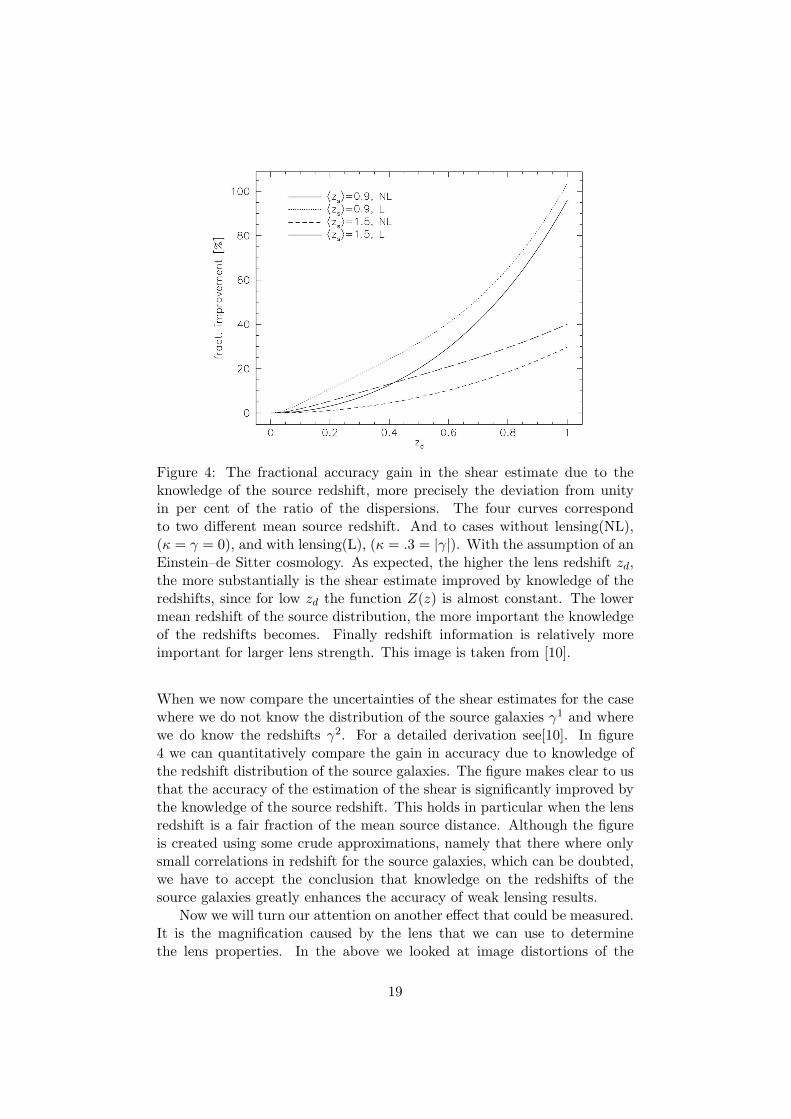
Figure 4: The fractional accuracy gain in the shear estimate due to theknowledge of the source redshift, more precisely the deviation from unityin per cent of the ratio of the dispersions. The four curves correspondto two different mean source redshift. And to cases without lensing(NL),(κ = γ = 0), and with lensing(L), (κ = .3 = |γ|). With the assumption of anEinstein–de Sitter cosmology. As expected, the higher the lens redshift zd,the more substantially is the shear estimate improved by knowledge of theredshifts, since for low zd the function Z(z) is almost constant. The lowermean redshift of the source distribution, the more important the knowledgeof the redshifts becomes. Finally redshift information is relatively moreimportant for larger lens strength. This image is taken from [10].

When we now compare the uncertainties of the shear estimates for the casewhere we do not know the distribution of the source galaxies γ1 and wherewe do know the redshifts γ2. For a detailed derivation see[10]. In figure4 we can quantitatively compare the gain in accuracy due to knowledge ofthe redshift distribution of the source galaxies. The figure makes clear to usthat the accuracy of the estimation of the shear is significantly improved bythe knowledge of the source redshift. This holds in particular when the lensredshift is a fair fraction of the mean source distance. Although the figureis created using some crude approximations, namely that there where onlysmall correlations in redshift for the source galaxies, which can be doubted,we have to accept the conclusion that knowledge on the redshifts of thesource galaxies greatly enhances the accuracy of weak lensing results.

Now we will turn our attention on another effect that could be measured.It is the magnification caused by the lens that we can use to determinethe lens properties. In the above we looked at image distortions of the

19

ellipticities of the source galaxies. We will look in detail into the change inthe number density of galaxies. Let n0(> S, z)dz be the number density ofgalaxies with redshift within dz of z and with a flux larger than S. Now atsome position ~θ we can write for the number counts according to (60),

n(> S, z) =1

µ(~θ, z)n0

(>

S

µ(~θ, z)

). (63)

This equation implies that magnification effects can either increase or de-crease the local number of counts. This depends on the shape of the unlensednumber–count function. This change of number counts is called magnifica-tion bias, and is important for gravitational lensing of QSOs. As statedearlier, magnification allows the observation of fainter sources. We have,

p(z;> S, κ, γ) =n0

[> µ−1(z)S, z

]µ(z)

∫dz′µ−1(z′)S, z′

, (64)

which is in analogy to equation (61) at fixed flux. Since we are dealingwith very faint objects here, spectroscopic information is hard to obtain.Therefore one can only observe the redshift–integrated counts,

n(> S) =∫

dz1

µ(z)n0(> µ−1(z)S, z). (65)

From observational evidence it follows that the number counts of faint galax-ies closely follow a power law over a wide range of fluxes. This allows us towrite the unlensed counts as,

n0(> S, z) = αS−αp0(z;S), (66)

where the exponent α depends on the wave band of the observation, andp0(z;S) is the redshift probability distribution of galaxies with flux> S. Theratio of the lensed and unlensed source counts is then found by insertingthe power law behavior of the unlensed number density into the redshiftintegrated counts,

n(> S)n0(> S)

=∫

dz µα−1(z)p0(z;µ−1S). (67)

Note that the lensed counts do not strictly follow a power law in S, sincep0 depends on z. The redshift distribution p0(z, S) is currently unknown,therefore the change of the number counts due to the magnification cannotbe predicted. For faint flux thresholds the redshift distribution is likelyto be dominated by galaxies at relative high redshift. For lenses at fairlysmall redshift of about zd ≤ 0.3, we can approximate the redshift–dependent

20

magnification by the magnification µ of a fiducial source at infinity, in whichcase,

n(> S)n0(> S)

= µα−1, (68)

which gives us a local estimation of the magnification. In the absence ofshape information and in the limit of weak gravitational lensing we haveµ ≈ (1 + 2κ) and we can obtain an estimate of the surface mass density,

κ ≈ n(> S)− n0(> S)n0(> S)

12(α− 1)

. (69)

Now that we have two independent methods to obtain estimates aboutthe mass distribution in the lensing plane it is interesting to compare thosetwo methods. Thus, we are going to compare the method that is based onshear measurements, and the one based on the number of counts. Considera small patch of the sky that contains N galaxy images in the absence ofgravitational lensing. The patch that we are considering must be sufficientlysmall to make sure that the lens parameters can be assumed to be constant.The dispersion of a shear estimate from averaging over galaxy ellipticities isσ2ε /N so that the signal–to–noise ratio is,(

S

N

)shear

=|γ|σε

√N. (70)

According to equation (69), the expected change in galaxy number counts is|∆N | = 2κ |α− 1|N . Assuming Poissonian noise, the signal–to–noise ratioin this case is, (

S

N

)counts

= 2κ |α− 1|√N. (71)

Upon comparison we find,

(S/N)shear(S/N)counts

=|γ|κ

12σε |α− 1|

. (72)

For situations such that κ ≈ |γ|, the above equation implies that the signal–to–noise ratio of the shear measurement is considerably larger that that ofthe magnification. Even for number–count slopes as flat as α ≈ 0.5, thisratio is larger than five, with σε ≈ 0.5. This leads us to conclude that shearmeasurements yield more significant results than magnification measure-ments. But there is more to this. Let make some additional considerations.Another argument to favor the shear measurements over the magnificationmeasurements is that we have a precise expectation in the absence of lens-ing for the shear measurements. The other method needs to compare the

21

measurements with calibration fields that are not lensed, which requires ac-curate photometry. Second, equation (71) overestimates the signal–to–noiseratio since we assumed errors in a Poissoin–like fashion. But real galaxiesare known to cluster even at very faint magnitudes, and so the error is un-derestimated. This is why most weak lensing measurements are done usinggalaxy ellipticities.

22

Observations

Now we are going to discuss some observations based on gravitational lens-ing. First, we will discuss the observations made by Clowe et al.[13], thatused weak gravitational lensing to prove the existence of dark matter di-rectly. The second we are going to discuss by Massey et al.[14]. This paperdeals with large scale three–dimensional structures in the universe. Thethree–dimensional maps are created using weak gravitational lensing analy-sis.

A direct empirical proof of the existence of dark matter

In this section we discuss an application of the theory we have outlined inthe preceding section. The article by Clowe et al.[13] claims to have founddirect empirical evidence that dark matter exists. And no alterations tothe gravitational force law are needed. They present weak lensing measure-ments of 1E0657–558 (z = 0.296), also known as the Bullet Cluster. Thissystem exhibits an unique feature. It consists of two galaxy clusters thatare merging. During the merger of the two clusters the individual galaxiesbehave as collisionless particles. But the intracluster gas that is existentin both clusters, experiences ram pressure. This implies that during a col-lision the gas and galaxies will decouple spatially. This effect can clearlybe seen in figure 5 of the Bullet Cluster. The geometry of this cluster pro-vides a good opportunity to test the dark matter hypothesis using weakgravitational lensing. As described in the above weak gravitational lensingis capable of tracing the mass distribution of the lensing cluster. We cannow discriminate between two different cases. The first case is without darkmatter. Without dark matter the gravitational potential will be dominatedby the mass of the colliding gas. For the second case, where dark matteris conjectured, we expect that weak lensing will show that the gravitationalpotential follows the distribution of the cluster cores. This because darkmatter will behave as collisionless matter. In their paper Clowe et al. useshear measurements to reconstruct the dimension–less surface mass densityκ. The peaks in the κ reconstruction are 8σ away from the centers of theplasma clouds. The orientation of those peaks is skewed towards the centersof the plasma peaks due to the fact that the plasma contributes about 10%

23

Figure 5: The Bullet Cluster, 1E0657–558. In the left panel is a color imagefrom the Magellan telescopes. The right panel is a 500 ks Chandra imageof the cluster showing the X–ray emission from the hot gas. In both panelsthe white bar indicates 200 kpc at the distance of the cluster. Also shownin both panels are reconstructed κ contour levels. These contours, obtainedfrom weak lensing observations, correspond to κ = 0.16 in the other contourand in increasing steps of κ = 0.07 towards the centers. The white contoursindicate the errors on the positions of the κ peaks. The contours correspondto 68.3%, 95.5% and 99.7% confidence levels. The two +s are added to markthe position of the centers of the plasma clouds. These images stronglysuggest that the mass density follows the galaxy centers, thus favoring ascenario with dark matter. These images were taken from[13].

of the total cluster mass. Note that both the plasma mass and the stellarmass are obtained directly from X–ray and optical images. Therefor theyare independent of any gravity of dark matter model. Within the standardcosmological framework including dark matter the observed κ distributionis another piece of evidence for the existence of dark matter. But let uslook at the possibility of explaining the observations on the Bullet Clusterwithin the MOND paradigm, or its relativistic extension TeVeS[4]. Withinthe TeVeS framework another κ map can be derived from the measurements.Without dark matter, the modifications to the theory of gravity should ex-plain the discrepancy of location in both the plasma and galaxy peaks. Dueto the geometry of the sytstem TeVeS needs to postulate a disk of gas be-tween the two mass concentrations that correspond to the subclusters. Themeasurements indicate that such a concentration is non–existent. This leadsto the conclusion that every modified theory of gravity that scales with thebaryonic mass fails to reproduce the correct results. In other words, in or-der to explain the observations modified gravity theories need to rely onadditional dark matter. Concluding the paper ends with the justificationof its title, the observed displacement between the bulk of the baryons andthe gravitational potential proves the presence of dark matter for the mostgeneral assumptions regarding the behaviour of gravity.

24

Figure 6: The redshift dependence of probes of large scale structure. Thesolid blue line represents the distribution of photometric redshifts for thesource galaxies. The solid black line shows the sensitivity of weak lensingmeasurements. The red line shows the sensitivity of X–ray detections. Imagetaken from [14].

Breaking the mass sheet degeneracy

The largest part of this paper over weak gravitational lensing dealt with twodimensional reconstructions of the mass distribution in the lensing plane.There are methods to break free from this two dimensional flatland andexplore three dimensional space. Here we are going to touch upon this sub-ject. We proceed by discussing the paper by Massey et al.[14]. In the sectionwhere we outlined the basic theory describing weak gravitational lensing wealready pointed out the fact that the dimension–less surface mass densityκ is redshift dependent. This dependency we are going to exploit here toconstruct a three dimensional map of the (dark) matter distribution. Pho-tometric redshift information about the source galaxies allows us to breakthe mass sheet degeneracy. In figure 6 the sensitivity of probes of large scalestructure as a function of distance is showed. In order to create a 3D distri-bution of dark matter we have to put or source galaxies into redshift bins.The quality of the photometric information about the source galaxies allowsus to put the source galaxies in redshift bins of ∆z = 0.05. Shear mea-surements of the galaxies in these bins can be used to construct the κ map.Putting together all those slices yields a 3D image of the matter distribu-tion. This distribution shows matter filaments in our universe. This matterdistribution corresponds to the large scale distribution of baryonic matter.In figure 7 the distribution is shown. The two pictures that appeared in thissection are taken from[14].

25

Figure 7: 3D reconstruction of the dark matter distribution. Axes corre-spond to Right Ascension, Declination, and Redshift. An isodensity contourhas been drawn at a level of 1.6×1012Msun within a circle of radius 700kpc.The image was construct using redshift bins ∆z = 0.05. The backgroundgrey scale corresponds to the local density. Image taken from [14].

26

Conclusion

In this paper we introduced the basic notions of weak gravitational lens-ing. The method of weak gravitational lensing is recognized to be one ofthe most reliable methods to determine the mass density of clusters. Thereliability of this method comes from its freedom from assumptions aboutthe physical state or the symmetries of the system. Next we introduced thedeflection potential, the shear and magnification. We considered two meth-ods to construct the dimension–less surface mass density. The first basedon the increase in number density, the second on the shear. We showedthat the method that was based on the shear measurements has a highersignal–to–noise ratio. Furthermore, the shear measurements do not need ad-ditional surveys of unlensed galaxies to compare with the lensed ones. Thenwe considered two papers that used the weak lensing shear analysis to drawconclusions that are cosmologically relevant. The first paper offered furtherproof that dark matter is real, and abundant in our universe. The othervisualized the invisible dark matter and demonstrated that the distributionof dark matter shows similarities in structure with the visible baryonic massdistribution.

27

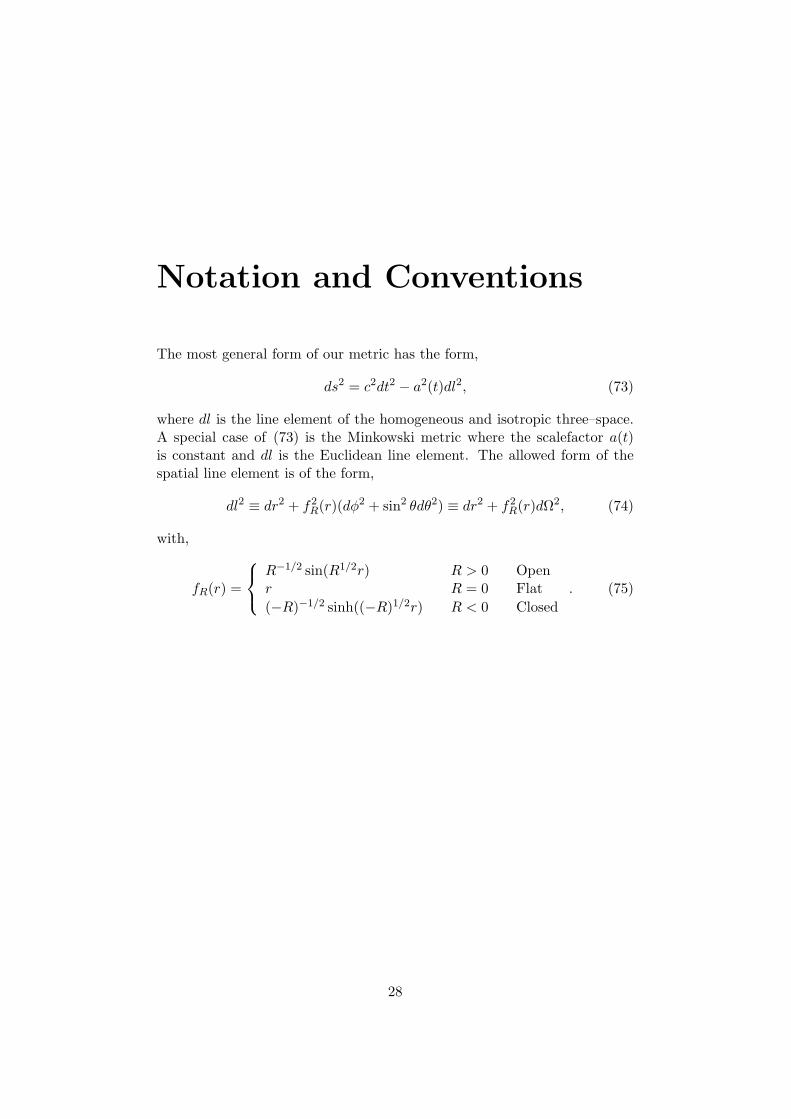
Notation and Conventions

The most general form of our metric has the form,

ds2 = c2dt2 − a2(t)dl2, (73)

where dl is the line element of the homogeneous and isotropic three–space.A special case of (73) is the Minkowski metric where the scalefactor a(t)is constant and dl is the Euclidean line element. The allowed form of thespatial line element is of the form,

dl2 ≡ dr2 + f2R(r)(dφ2 + sin2 θdθ2) ≡ dr2 + f2

R(r)dΩ2, (74)

with,

fR(r) =

R−1/2 sin(R1/2r) R > 0 Openr R = 0 Flat(−R)−1/2 sinh((−R)1/2r) R < 0 Closed

. (75)

28

Bibliography

[1] Zwicky, F. 1933. Die Rotverschiebung von extragalaktischen Nebeln,Helvetica Physica Acta 6: 110127.

[2] Rubin, V.C, Ford Jr WK. 1970. Ap. J. 159:379

[3] Wayne Hu & Scott Dodelson. Cosmic Microwave BackgroundAnisotropies. 2002. Ann. Rev. A&A. 40: 171–216. e–Print: Arxiv:Astro–ph/0110414.

[4] Jacob. B. Bekenstein. The modified Newtonian dynamics–MOND andits implications for new physics. 2006. Contemporary Physics 47, 387.Arxiv: Astro–ph/0701848.

[5] Thomas Rot, Modified Newtonian Dynamics: a possible solutionto the dark matter problem, Seminar cosmology, 2009. e–Print:http://www.phys.uu.nl/∼prokopec/ThomasRot mond2.pdf

[6] Tomislav Prokopec, Lecture notes on Cosmology I. 2007. e–Print:http://www.phys.uu.nl/∼prokopec/1gr.pdf.

[7] Dyson, F. Eddington, A. Davidson C. 1920. A Determination of theDeflection of Light by the Sun’s Gravitational Field, from ObservationsMade at the Total Eclipse of May 29, 1919. Phil. Trans. Roy. Soc. A220:291–333.

[8] Schneider, P. & Seitz, C., Steps toward nonlinear cluster inversionthrough gravitational distortions, 1995, A&A 320, 411.

[9] Schneider P., Weak Gravitational Lensing, 2005, Arxiv:Astro–ph/0509252.

[10] Bartelmann M. & Schneider P., Weak gravitational lensing, 2001, Phys.Rept. 340, 291–472.

[11] Seitz, C. & Schneider, P., 1997, A&A, 318,687

[12] Dipak Munshi, Patrick Valageas, Ludovic van Waerbeke, Alan F. Heav-ens, Cosmology with Weak Lensing Surveys. 2008, Phys. Rept. 462:67–121. Arxiv:astro–ph/0612667.

29

[13] Douglas Clowe, Marusha Bradac, Anthony H. Gonzalez, Maxim Marke-vitch, Scott W. Randall, Christine Jones and Dennis Zaritsky. A directempirical proof of the existence of dark matter, 2006. Astrophysical J.648 L109–L113. e–Print: http://arxiv.org/abs/astro–ph/0608407.

[14] Richard Massey, Jason Rhodes, Richard Ellis, Nick Scoville, AlexieLeauthaud, Alexis Finoguenov, Peter Capak, David Bacon, Herve Aus-sel, Jean–Paul Kneib, Anton Koekemoer, Henry McCracken, BahramMobasher, Sandrine Pires, Alexandre Refregier, Shunji Sasaki, Jean–Luc Starck, Yoshi Taniguchi, Andy Taylor & James Taylor. 2007. Darkmatter maps reveal cosmic scaffolding, Nature, 445: 286.

30