self-taught learning a dissertation...
TRANSCRIPT

SELF-TAUGHT LEARNING
A DISSERTATION
SUBMITTED TO THE DEPARTMENT OF COMPUTER SCIENCE
AND THE COMMITTEE ON GRADUATE STUDIES
OF STANFORD UNIVERSITY
IN PARTIAL FULFILLMENT OF THE REQUIREMENTS
FOR THE DEGREE OF
DOCTOR OF PHILOSOPHY
Raj at Raina
September 2009

UMI Number: 3382948
Copyright 2009 by Raina, Rajat
INFORMATION TO USERS
The quality of this reproduction is dependent upon the quality of the copy
submitted. Broken or indistinct print, colored or poor quality illustrations
and photographs, print bleed-through, substandard margins, and improper
alignment can adversely affect reproduction.
In the unlikely event that the author did not send a complete manuscript
and there are missing pages, these will be noted. Also, if unauthorized
copyright material had to be removed, a note will indicate the deletion.
®
UMI UMI Microform 3382948
Copyright 2009 by ProQuest LLC All rights reserved. This microform edition is protected against
unauthorized copying under Title 17, United States Code.
ProQuest LLC 789 East Eisenhower Parkway
P.O. Box 1346 Ann Arbor, Ml 48106-1346

© Copyright by Raj at Raina 2009
All Rights Reserved

I certify that I have read this dissertation and that, in my opinion, it
is fully adequate in scope and quality as a dissertation for the degree
of Doctor of Philosophy.
(Andrew Y. Ng) Prmoapal Adviser
I certify that I have read this dissertation and that, in my opinion, it
is fully adequate in scope and quality as a dissertation for the degree
of Doctor of Philosophy
(Daphne Koller)
I certify that I have read this dissertation and that, in my opinion, it
is fully adequate in scope and quality as a dissertation for the degree
of Doctor of Philosophy.
(Krishna Shenoy)
Approved for the University Committee on Graduate Studies.
^ f e - . ^ . A#~y^*~
i i i
Acknowledgement
My journey at Stanford has benefitted greatly from the support of many people. First
and foremost, it has been a privilege to have Andrew Ng as my advisor. Andrew has
been a constant source of research advice and ideas. I am grateful that he made sure
his students always had the resources, support and motivation they needed to excel.
And above all, Andrew has been a wonderful and inspirational mentor. I will cherish
and remember his advice for a long time to come.
Over the years, I have had several helpful discussions with professors at Stanford. I
am especially grateful to Daphne Koller for her advice and for being on my dissertation
reading committee. I have had several stimulating discussions with Krishna Shenoy
and I thank him for being on my dissertation reading committee. I thank Christopher
Manning for his guidance in my early formative years at Stanford, and Benjamin van
Roy for being a wonderful teacher. I am grateful to Trevor Hastie for chairing my
Orals committee.
I am indebted to my fellow students at Stanford for helping shape my research.
I especially acknowledge Honglak Lee and Roger Grosse for collaborating closely on
various projects. Their ideas and diligence have had a huge impact on the work
presented here. I thank Ian Goodfellow and Quoc Le for help with installing graphics
processor hardware. I have greatly enjoyed collaborating with Alexis Battle, Anand
Madhavan and Benjamin Packer on various topics discussed in this thesis. I thank
Adam Coates, Ashutosh Saxena, Chuong Do, Pieter Abbeel, Rion Snow, Stephen
Gould and Zico Kolter for the many enlightening discussions.
Life has been fun at Stanford, and I owe that largely to my friends. If you are
reading this, you probably know who you are. Thank you.
IV

My family has stood by my side throughout my journey at Stanford. I am indebted
to Rahul and Nirmala for being my friends over the years, and to Ajju for being a
constant source of peace and happiness.
My biggest achievement at Stanford has to be that I found Penka. What would I
have done without her?
Finally, my parents Rajni and Vijay made me what I am. For their unconditional
support, guidance and love, this thesis is dedicated to them.
v

Contents
Acknowledgement iv
1 Introduction 1
1.1 Supervised learning 1
1.2 Feature engineering 3
1.3 More data, less feature engineering 4
1.3.1 Semi-supervised learning 5
1.3.2 Transfer learning 9
1.4 Self-taught learning 10
1.5 Automatic feature construction methods 14
1.6 Unsupervised feature construction methods 16
1.6.1 Text documents 19
1.6.2 Computer vision 22
1.6.3 Discussion 23
1.7 Summary of contributions 25
1.7.1 Self-taught learning 25
1.7.2 Algorithms for self-taught learning 25
1.7.3 Self-taught learning for audio classification 26
1.7.4 Self-taught learning for discrete inputs 27
1.7.5 Large-scale deep unsupervised learning 28
1.8 First published appearances of the described work 29
vi

2 Self-taught Learning 31
2.1 Problem Formalism 31
2.2 A Self-taught Learning Algorithm 32
2.3 Learning higher-level representations 33
2.3.1 Sparse Coding 35
2.3.2 A different sparse coding formulation 36
2.4 Unsupervised Feature Construction 39
2.5 Comparison with Related Methods 44
2.6 Experiments 53
2.6.1 Implementation details 53
2.6.2 Results 56
2.6.3 Other methods of using unlabeled data 60
2.7 A classifier for sparse coding features 63
2.7.1 A probabilistic model for sparse coding 64
2.7.2 Obtaining a classifier for sparse coding 67
2.7.3 Experimental comparison 69
2.8 Discussion 69
2.8.1 Biological comparisons 70
2.8.2 Theoretical guarantees 71
2.8.3 Extensions to the sparse coding model 73
3 Self-taught Learning for Audio Classification 75
3.1 Shift-invariant Sparse Coding 78
3.2 Efficient SISC Algorithm 79
3.2.1 Solving for activations 80
3.2.2 Solving for basis vectors 83
3.3 Constructing features using unlabeled data 87
3.4 Algorithm Efficiency 90
3.5 Self-taught Learning Results 91
3.6 Discussion 96
vn

4 Self-taught Learning for Discrete Inputs 98
4.1 A probabilistic model for sparse coding 100
4.2 Self-taught Learning for Discrete Inputs 101
4.3 Exponential Family Sparse Coding 102
4.3.1 Computing optimal activations 104
4.3.2 Computational Efficiency 106
4.4 Application to self-taught learning 110
4.4.1 Text classification 110
4.4.2 Robotic perception 114
4.5 Discussion 115
5 Large-scale Deep Unsupervised Learning 117
5.1 Deep learning algorithms 118
5.2 Large-scale learning 120
5.3 Computing with graphics processors 122
5.4 Preliminaries 124
5.4.1 Deep Belief Networks 124
5.4.2 Sparse Coding 125
5.5 GPUs for unsupervised learning 126
5.6 Learning large deep belief networks 128
5.6.1 Experimental Results 130
5.7 Parallel sparse coding 133
5.7.1 Parallel Li-regularized least squares 134
5.7.2 Experimental Results 135
5.8 Discussion 136
6 Conclusions 138
vm

List of Tables
2.1 Details of self-taught learning applications evaluated in the experiments. 54
2.2 Classification accuracy for self-taught learning on the Caltech 101 im
age classification dataset 57
2.3 Classification accuracy for self-taught learning on character images. . 58
2.4 Classification accuracy for self-taught learning on music genre classifi
cation 59
2.5 Example sparse coding basis vectors learned on text documents. . . . 59
2.6 Classification accuracy for self-taught learning on text classification. . 60
2.7 Control experiment: Classification accuracy when sparse coding or
PCA are applied to labeled data 61
2.8 Classification accuracy for self-taught learning using the learned sparse
coding kernel classifier 69
3.1 Classification accuracy of shift-invariant sparse coding on music genre
classfication 95
3.2 Classification accuracy of shift-invariant sparse coding on speaker iden
tification 96
4.1 Experiment comparing running time of algorithms for computing acti
vations in binary sparse coding 108
4.2 Experiment comparing running time of algorithms for parameter learn
ing for Li-regularized logistic regression benchmarks 109
4.3 Illustration of exponential family sparse coding basis vectors learned
for text documents I l l
IX

4.4 Classification accuracy of exponential family sparse coding on text clas
sification tasks 112
4.5 Classification accuracy of exponential family sparse coding on a robotic
perception task 115
5.1 A rough estimate of number of free parameters in some recent published
work on deep belief networks 121
5.2 Experiment comparing running time of GPU-based algorithm for learn
ing a large restricted Boltzmann machine 131
5.3 Experiment comparing running time of GPU-based algorithm for learn
ing a large overlapping patch model for a deep belief network 132
5.4 Experiment comparing running time of GPU-based algorithm for solv
ing the sparse coding optimization problem 135
x

List of Figures
1.1 Illustration of machine learning formalisms related to self-taught learning. 11
2.1 An illustration of the idea behind our algorithm for learning higher-
level representations 34
2.2 Example sparse coding results for image and audio inputs 40
2.3 An illustration of the idea behind the sparse coding algorithm for un
supervised feature construction 42
2.4 Example sparse coding features computed for image classification. . . 43
2.5 Illustration of basis vectors learned by PCA, PCA with sparsity, and
sparse coding 50
2.6 Example images and sparse coding basis vectors for the character image
datasets 58
2.7 Probabilistic model for sparse coding 65
3.1 Illustration of shift-invariant sparse coding for audio 77
3.2 Experiment comparing running time of shift-invariant sparse coding
algorithms 92
4.1 Illustration of the IRLS-FS algorithm for Li-regularized optimization. 106
4.2 Classification accuracy of exponential family sparse coding on text clas
sification tasks 113
4.3 Illustration of point-cloud and spin-image inputs for robotic perception. 114
5.1 Simplified schematic for the Nvidia GeForce GTX 280 graphics card. 122
XI

5.2 Schematic diagram of the overlapping patches model for deep belief
networks 129
xn

Chapter 1
Introduction
We introduce a new machine learning framework called self-taught learning. Algo
rithms in the self-taught learning framework require almost no human supervision,
and can learn from easily available data sources. Machine learning algorithms are
often only as good as the data they can learn from. Since self-taught learning algo
rithms can learn from much more data than many conventional learning algorithms,
we believe that the development of such algorithms can significantly improve prac
tical applications of machine learning. In this thesis, we develop several self-taught
learning algorithms, and show that these algorithms work well on a wide variety of
machine learning applications.
1.1 Supervised learning
In recent years, machine learning techniques have been used in large variety of appli
cations, including computer vision, natural language processing, speech recognition,
and recommendation systems. The vast majority of these applications rely on using
labeled training data to train models. For example, state-of-the-art methods for rec
ognizing face images rely on being trained using thousands of labeled face images;
methods for document categorization use thousands of documents already labeled
with the target categories; and methods for speech recognition are trained on anno
tated speech samples from many users.
1

CHAPTER 1. INTRODUCTION 2
The task of learning from labeled data is called supervised learning, and has
been widely studied in machine learning and statistics. Over the past few decades,
many sophisticated learning methods have been developed for supervised learning
problems—support vector machines (Cortes & Vapnik, 1995), conditional random
fields (Lafferty et al., 2001), generalized linear models (McCullagh & Nelder, 1989),
neural networks (Rumelhart et al., 1987), to name just a few—and they are able to
achieve good performance in a wide variety of fields. At their heart, these methods
rely on being given a large number of training inputs x E X, with their known labels
y E y, which they then use to fit a function h : X —» y that approximates the
mapping from inputs to labels; once the function h is obtained on the labeled train
ing data, we can take a new, previously unseen input xnew G X and predict a label
M^new) f° r that input. When a sufficiently large number of labeled training examples
is available, supervised learning methods are often able to learn good predictors that
give very accurate predictions on new examples. In many cases, the performance of
these predictors can be theoretically guaranteed (under some assumptions).
The most challenging problems in machine learning arise when the number of
labeled examples is "small." To take a specific example, consider a computer vision
application, where we have to predict the gender (male or female) of a person from
a 100 x 100 pixel input image of their face. Each input image can be represented as
a high-dimensional vector x G R10000, containing the pixel intensities of each of the
10,000 pixels in the image. In principle, it should be possible to fit a function h
that takes these 10,000-dimensional input vectors and predicts whether the person
in the image is male or female. In practice, this can be quite hard: a slight shift in
the camera angle, or lighting conditions, or facial expression, can change the 10,000
numbers (pixel intensity values) dramatically; in the face of all these variations, we
need the function h to somehow sift through all of the unimportant changes in pixel
values, and compute an aggregate function that captures just the gender represented
by the pixels. To have any hope of recovering such a function h, it appears that we
would need to fit the function using thousands of labeled examples, at least. When
many fewer labeled examples are available (e.g., tens of gender-labeled face images),
the straightforward supervised learning approach does not work as well.

CHAPTER 1. INTRODUCTION 3
Unfortunately, it can often be difficult to obtain sufficiently large amounts of la
beled data for supervised learning. Labeled data typically requires human supervision
(e.g., a human looking at thousands of face images, and labeling each as male or fe
male), which makes it very expensive to produce. It is thus highly desirable to have
machine learning methods that are able to learn with very few labeled examples, and
with limited human supervision. This is especially true for modern applications, such
as on those on the web or on mobile devices, where we often want to learn a good
predictor from very few user interactions.
1.2 Feature engineering
With limited labeled data, since the supervised learning task is often hard to solve
automatically, one possible approach is to build in more knowledge into the supervised
learner. Instead of taking the raw inputs x & X and labels y E y, we might manually
compute certain functions $(x), called "features," of the input that we think are
informative in predicting the label y. In the previous example, we represented each
face image by a vector x € R10000; this is a fairly impoverished representation in
terms of raw pixel intensities, with no knowledge encoded about images in general
(e.g., that they often have slowly varying regions separated by edges) or about faces
in particular (e.g., that they have two eyes and a nose). We might instead use image
processing techniques to compute image functions such as:
• $i(x) = (The distance between the eyes)2 / (The length of the nose)
• $2 (a) = The length of the hair.
• $3(2;) = The width of the forehead.
• . . .
• $10 (x) = The angle of the chin.
It is tough to write down new features like these that are indeed informative about the
gender, and designing good features often requires significant human expertise, insight

CHAPTER 1. INTRODUCTION 4
and ingenuity. Also, some features are themselves hard to compute—for example, it
is not immediately clear how we could find the exact location of the eyes, given only
10,000 numbers representing pixel intensities for the face. In fact, some of these
features might themselves require years of image processing research to compute
accurately, even for this one application domain. Once we have the output of these
features $(x), we might finally hope to be able to learn a function p($(x)) that
uses the computed features $(x) (consisting of 10 numbers) instead of the original
10,000-dimensional input space to much more easily predict the gender label y.
This approach to machine learning is not completely satisfactory—we set out to
automatically learn about images (or audio, or text, etc.), but in the end, had to spend
significant amounts of time manually designing features that would enable learning
algorithms to find good predictors. Many of these hand-engineered features are highly
specific to particular applications, and may not easily carry over to new application
domains. Further, feature design is often an empirical process, that is driven at best
by human intuition, and at worst by plain trial and error. Some features might be
informative and useful when considered individually, but might be subsumed by other
features when considered all-at-once. Humans are exceptionally good at predicting
the gender given a face image, but they still may not be able to write down 10
numbers (features) that led them to making their predictions.1 Informally, humans
are not very good at number crunching, and this can make feature engineering a
laborious and cumbersome process.
This example suggests that to apply supervised learning to many hard, new prob
lems, we might need to invest several person-years into intensive research to develop
high-quality features, before learning can be successfully applied.
1.3 More data, less feature engineering
The above discussion leads to one of the central problems in machine learning over
the past decade: given that labeled data is expensive and hard to obtain, can we
1For this particular problem, there are even detailed experiments studying the visual cues that humans use to perform gender discrimination. (Dupuis-Roy et al., 2009)
CHAPTER 1. INTRODUCTION 5
use other, more easily available sources of data for learning? The hope is that by
using these other sources of data to guide the learning process, we might be able get
away with less labeled data, and less feature engineering. This has led to whole new
ways of thinking about machine learning, and given rise to significant new machine
learning formalisms, that go beyond supervised learning. We briefly discuss two
relevant formalisms.
1.3.1 Semi-supervised learning
In many machine learning applications, it is hard to get labeled data, but it is rela
tively easy to get large amounts of unlabeled data. For face recognition, it is possible
to get a large number of face images automatically (e.g., by running a simple face de
tector over images)—each of these images contains a face, we just don't know whether
it is a male or a female face. One might imagine that by looking at a large number of
such unlabeled input examples xu G X, even without the corresponding labels yu G y,
we can learn useful things about the input domain. For example, we can estimate
the input-only or "marginal" distribution P(x), which might inform our supervised
learning algorithm that some x values, or some combinations of 10,000 pixel intensity
values, are more likely to represent faces than others; by then focusing our function-
fitting and learning algorithm on those parts of the input space only, we might obtain
a simpler supervised learning problem, and we might be able to learn a better predic
tor. Viewed another way, having access to a large number of unlabeled face images
xu G X might help us "expand" our labeled training set by finding images that are
extremely similar to certain labeled face images; if an unlabeled image is extremely
similar to a labeled image, it appears reasonable to assume that the unlabeled image
has the same label. This effectively gives us more information about the mapping
x —> y that we can use for learning.
This formalism of using both labeled and unlabeled data to solve a supervised
learning problem is called semi-supervised learning, as it is in between supervised
learning (only labeled data) and unsupervised learning (only unlabeled data). It
assumes that the unlabeled data is derived from the same classes as the labeled data;

CHAPTER 1. INTRODUCTION 6
each unlabeled example xu e X can be assigned a valid label yu e y in principle, but
the label is just not available for learning. This makes sense for some applications:
in our running example, any unlabeled face image must be either male or female, we
just don't know the label. This turns out to be an important aspect of several semi-
supervised learning algorithms, and one that we will return to later in the section.
There are tens of published papers on semi-supervised learning algorithms, and we
refer the reader to Zhu's survey paper (Zhu, 2005) and Chapelle et al.'s book (Chapelle
et al., 2006) for a comprehensive overview. To help later discussion, we give a bird's
eye view of the field. If we consider supervised learning algorithms as attempting to
find predictor functions h that minimize some "loss function" C (such as squared-
error, misclassification rate, etc.) on the labeled data: a rgmin/£( / ) , then loosely
speaking, semi-supervised learning algorithms attempt to influence this process in
various ways, by using various notions of what a "good" predictor should do on the
unlabeled data. To name just a few:
• A good predictor should suggest label boundaries only in areas of low input den
sity P(x), so that most inputs x € X lie far from the label boundary. Intuitively,
this gives the predictor some margin for error, and makes the predictions more
likely to be correct. This is often also called the "cluster assumption." (Seeger,
2001) Some methods, such as transductive support vector machines (Vapnik,
1998; Joachims, 1999), attempt to directly capture this assumption in picking
the supervised learning predictor.2 Several other methods use this intuition to
pose different models, including via Gaussian processes (Lawrence & Jordan,
2006) or information regularization (Szummer & Jaakkola, 2003).
• A good predictor should vary "smoothly" in its predictions on the unlabeled
data—if two unlabeled examples x\ and x\ are very similar, then the predictions
h(xl) and h(x%) should also be similar. A large number of semi-supervised
learning methods construct a weighted graph over input examples (with weights
specifying similarities), and then formalize the algorithm using graph-theoretic
technically, transductive learning can be considered a special case of semi-supervised learning, where the unlabeled inputs are exactly the ones that we need predictions for. For our purposes, this is not a very important distinction.

CHAPTER 1. INTRODUCTION 7
notions of connectedness or smoothness (Blum & Chawla, 2001; Belkin et al.,
2005; Zhou et a l , 2003).
• If the supervised learning model attempts to learn a joint distribution P(x, y)
to capture what inputs x are likely to occur with what labels y, semi-supervised
learning provides information about the input distribution P(x), which might
inform us about the predictive distribution P(y\x). Such information can be
leveraged, for example, by "guessing" the likely labels yu for the unlabeled
inputs xu, and then using these labels for learning. (Nigam et al., 2006)
• A somewhat different method would be to use unlabeled data to learn an en
coding for inputs x, and then use that encoding to simplify the supervised
learning problem. For example, the input can be represented using a decompo
sition such as principal components analysis (PCA), which attempts to find a
low-dimensional subspace close to most input examples; representing each in
put example by its low-dimensional representation could then lead to a simpler
supervised learning problem.3 Many other methods fall in this category, in
cluding manifold learning methods such as ISOMAP (Tenenbaum et al., 2000)
and locally-linear embedding (Roweis & Saul, 2000), and several neural network
models that are contemporary to our work, including deep belief networks (Hin-
ton & Salakhutdinov, 2006) and autoencoders (Bengio et al., 2006). Instead of
finding structure in the inputs, a semi-supervised learning method can also at
tempt to learn structure within good predictors h, often over auxiliary learning
tasks constructed by applying heuristics to the unlabeled data; this structure
can be used to prefer predictors with the learnt structure. (Ando & Zhang,
2005)
This is not an exhaustive list of semi-supervised learning algorithms, but it is
worth pointing out that most of these algorithms make certain assumptions about
the problem at hand, and the nature of the unlabeled and labeled data. When these 3Such an application of principal components analysis is especially common for text documents,
where it can represent documents using semantically-meaningful combinations of words (subspaces in the input word space), instead of just using the individual words. For text documents, this is often called latent semantic analysis. (Deerwester et al., 1990)

CHAPTER 1. INTRODUCTION 8
assumptions are valid, semi-supervised learning can often help predictive performance;
but when the assumptions are violated, semi-supervised learning can sometimes hurt,
by adding a flawed notion of good predictors to the supervised learning problem. (Coz-
man & Cohen, 2002)
For this thesis, we are interested in relaxing a central restriction made by many
semi-supervised learning algorithms: the unlabeled data must be from the same
classes as the labeled data. Further, many algorithms implicitly assume that the
unlabeled inputs xu are drawn from the same distribution as the labeled inputs, and
that estimating this common input distribution is useful for better learning. In many
real applications, these assumptions are unfortunately difficult to meet. Consider the
following examples of supervised learning tasks:
• Classifying images of elephants vs. images of rhinos: To apply semi-supervised
learning, the unlabeled data must consist of images just of elephants and rhinos
(and no other images). Given an unlabeled image and sufficient time, one should
be able to provide a label "elephant" or "rhino." This is unsatisfactory as it is
difficult to get truly unlabeled images of just elephants and rhinos, and nothing
else, in such a way that we don't already know the label. What we can get
easily are unlabeled images of jungles, or pictures of natural environments, but
these do not fit into the semi-supervised learning framework.
• Distinguishing between 5 specific speakers using their recorded speech: To apply
semi-supervised learning, we need unlabeled examples (speech) from exactly
those 5 speakers. This is not very helpful—if we could record from one of those
5 speakers, we would just have more labeled data, not more unlabeled data.
Instead, the "unlabeled data" we might want to use would be speech samples
from other users, possibly speaking different languages, but semi-supervised
learning does not allow this.
• Categorizing webpages about pottery vs. webpages about sculptures: Again, it
is unclear how we can apply semi-supervised learning, because it appears hard
to get unlabeled webpages that are about pottery or sculptures, but nothing
else.

CHAPTER 1. INTRODUCTION 9
Thus, the semi-supervised learning framework does not seem to capture many
types of unlabeled data that we would like to use to help supervised learning. This is
a central observation and we will return to it later in proposing a different framework
for using unlabeled data in machine learning. We also discuss the application of some
semi-supervised learning methods and other prior art to our framework in Section 1.6,
and in further detail in Section 2.5.
1.3.2 Transfer learning
Recall the supervised learning problem, where we are given a classification task with
limited labeled data, and we would like to learn a good predictor from this data.
Transfer learning (sometimes called multitask learning) asks the following question:
can access to labeled data from other supervised learning problems help? Consider
our running example of predicting gender from a face image. If we are given access to
many other "similar" supervised learning problems (e.g., classifying elephant images
vs. rhino images, classifying car images vs. motorcycle images, etc.), we might be able
to discover the properties of "good predictors" for any of these tasks—for example,
a prediction probably should not change too much if we move the camera a little,
leading to a displacement of pixels in the image. By developing this notion of a good
predictor on the extra supervised learning problems, and then applying the notion
to help the supervised problem we care about (classifying face images), we might be
able to find better predictors. In this way, transfer learning might help in situations
with limited labeled data.
Again, many different algorithms have been devised for transfer learning, each
requiring somewhat different assumptions. (Thrun, 1996; Ando & Zhang, 2005; Caru-
ana, 1997) For good transfer learning, we need the extra supervised learning tasks to
be "related" to the supervised learning task at hand, and this relatedness has been
quantified in theoretical terms. (Baxter, 1997)
However, to apply transfer learning, we require labeled data, even if from other
supervised learning problems. Given a new supervised learning problem, it can be
difficult to find related labeled data (and if we have to manually label related data,

CHAPTER 1. INTRODUCTION 10
we might as well label data for the supervised learning task at hand).
1.4 Self-taught learning
Self-taught learning is a formalism for using unlabeled data in machine learning. To
motivate our discussion, consider as a running example the computer vision task of
classifying images of elephants and rhinos. For this task, it is difficult to obtain many
labeled examples of elephants and rhinos; indeed, it is difficult even to obtain many
unlabeled examples of elephants and rhinos. (In fact, we find it difficult to envision a
process for collecting such unlabeled images, that does not immediately also provide
the class labels.) This makes the classification task quite hard with existing algo
rithms for using labeled and unlabeled data, including most semi-supervised learning
algorithms. (Nigam et al., 2000) Instead, we ask how unlabeled images from other
object classes—which are much easier to obtain than images specifically of elephants
and rhinos—can be used. For example, given unlimited access to unlabeled, ran
domly chosen images downloaded from the Internet (probably none of which contain
elephants or rhinos), can we do better on the given supervised classification task?
Although we use computer vision as a running example, the problem that we pose
to the machine learning community is more general. Formally, we consider solving
a supervised learning task given labeled and unlabeled data, where the unlabeled
data does not share the class labels or the generative distribution of the labeled data.
For example, given unlimited access to natural sounds (audio), can we perform better
speaker identification? Given unlimited access to news articles (text), can we perform
better webpage classification?
Like semi-supervised learning (Nigam et al., 2000), our algorithms will therefore
use labeled and unlabeled data. But unlike semi-supervised learning as it is typically
studied in the literature, we do not assume that the unlabeled data can be assigned
to the supervised learning task's class labels. To thus distinguish our formalism from
such forms of semi-supervised learning, we will call our task self-taught learning.
We compare our framework with transfer learning first. Given a supervised learn
ing problem with limited labeled data, transfer learning typically requires further
CHAPTER 1. INTRODUCTION 11
Supervised Classification Semi-supervised Learning
Transfer Learning Self-taught Learning
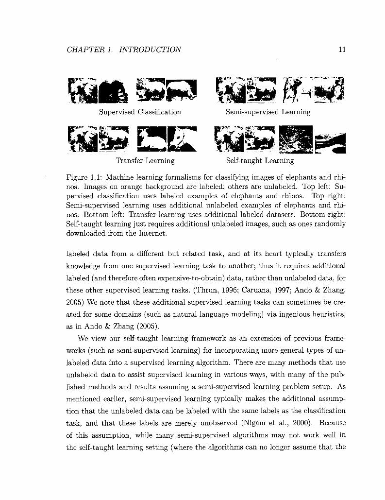
Figure 1.1: Machine learning formalisms for classifying images of elephants and rhinos. Images on orange background are labeled; others are unlabeled. Top left: Supervised classification uses labeled examples of elephants and rhinos. Top right: Semi-supervised learning uses additional unlabeled examples of elephants and rhinos. Bottom left: Transfer learning uses additional labeled datasets. Bottom right: Self-taught learning just requires additional unlabeled images, such as ones randomly downloaded from the Internet.
labeled data from a different but related task, and at its heart typically transfers
knowledge from one supervised learning task to another; thus it requires additional
labeled (and therefore often expensive-to-obtain) data, rather than unlabeled data, for
these other supervised learning tasks. (Thrun, 1996; Caruana, 1997; Ando & Zhang,
2005) We note that these additional supervised learning tasks can sometimes be cre
ated for some domains (such as natural language modeling) via ingenious heuristics,
as in Ando & Zhang (2005).
We view our self-taught learning framework as an extension of previous frame
works (such as semi-supervised learning) for incorporating more general types of un
labeled data into a supervised learning algorithm. There are many methods that use
unlabeled data to assist supervised learning in various ways, with many of the pub
lished methods and results assuming a semi-supervised learning problem setup. As
mentioned earlier, semi-supervised learning typically makes the additional assump
tion that the unlabeled data can be labeled with the same labels as the classification
task, and that these labels are merely unobserved (Nigam et al., 2000). Because
of this assumption, while many semi-supervised algorithms may not work well in
the self-taught learning setting (where the algorithms can no longer assume that the

CHAPTER 1. INTRODUCTION 12
unlabeled data comes from the classes in the supervised task), it is possible that
some semi-supervised algorithms can be successfully applied to self-taught learning
problems, or can be modified to work well on self-taught learning problems.
In conventional semi-supervised learning, we assume that the unlabeled data
comes from the same classes as the labeled data; in self-taught learning, we do not
require this assumption. Given a supervised learning task with many classes, we can
always add an extra "other" class, and assume that all the unlabeled data arises from
that class. Technically, this reduces the self-taught learning to a semi-supervised
learning problem, and so self-taught learning can be viewed as a specific type of semi-
supervised learning problem.4 But we note that in this reduction, the semi-supervised
learning problem contains all the unlabeled data from just one ("other") class, and
thus we do not expect the reduction to be practically useful in semi-supervised learn
ing algorithms.
Over the past decade, there has been extensive research on semi-supervised learn
ing methods (e.g., see survey papers by Seeger, 2001 and Zhu, 2005), and we discuss
related work at length in the following pages, but we make particular mention of two
published modifications for semi-supervised learning that appear most closely related
to the self-taught learning framework:
• Semi-supervised learning by learning predictive structures: Ando &
Zhang (2005) proposed a transfer learning method that attempts to use multiple
supervised learning tasks to learn the properties of good classifiers for these
tasks. While their method is based on labeled data from multiple learning tasks,
they show that for some domains, the labeled data for these multiple learning
tasks can be created automatically by applying heuristics to unlabeled data. For
example, given unlabeled text documents, we can hide the presence/absence of
a specific word w, and then label each document either as Y (if it contains the
word w) or N (otherwise); this heuristic procedure thus provides labeled data
for an artificially created supervised learning problem, to which the transfer
learning algorithms can be applied. Using such heuristics, we can thus use both 4This reduction was pointed out to us by Trevor Hastie.

CHAPTER 1. INTRODUCTION 13
unlabeled and labeled data in learning a good classifier. The authors show good
performance on semi-supervised learning for several text and language-related
tasks.
Ando k, Zhang's method can be extended to apply to several self-taught learning
problems, as long as we can construct a heuristic that can create the auxiliary-
labeled data. While they suggest such heuristics for language problems, new
heuristics need to be picked for new application domains, such as for image or
audio inputs.
• The Universum method: Among recent methods in the literature, the Uni-
versum method (Weston et al., 2006), developed contemporarily to our method,
appears to be closest in spirit to our self-taught learning framework. The Uni
versum is a collection of unlabeled examples that specifically do not belong to
the labeled classes of interest. For example, to learn a classifier to distinguish
between images of elephants and rhinos, the unlabeled data must not contain
any examples of elephants and rhinos. This assumption is different and more
restrictive than the assumptions we consider for self-taught learning. One ma
jor point of difference is that we expect self-taught learning algorithms to work
best in the semi-supervised learning setting (where the unlabeled data is from
the same classes as the labeled data, and is thus very "similar"), whereas the
definition of the Universum itself excludes the semi-supervised learning setting.
The specific algorithm presented by Weston et al. (Weston et al., 2006) for learn
ing with the Universum uses a modification of the cluster assumption—instead
of encouraging the learnt predictor to pass through low input density regions for
the original supervised learning problem, the algorithm encourages the learnt
predictor to pass through high input density regions for the Universum. Since
the Universum contains examples only from other classes, this encourages the
predictor to be ambivalent about those other classes. In contrast, the methods
we will consider for self-taught learning have a very different flavor. They rely
on using unlabeled data to learn good encodings (features) of the input, and
to then use these encodings for representing the labeled data. Instead of using

CHAPTER 1. INTRODUCTION 14
the distribution of the unlabeled inputs, the methods use the encoding of the
unlabeled input itself and try to find patterns that recur in many input exam
ples. In any case, it is possible that the algorithm developed for the Universum
problem can apply to some self-taught learning problems as well.
How do we use the unlabeled data in self-taught learning? To give a rough idea, it
is easiest to return to the discussion on feature-engineering earlier. We discussed ear
lier that given limited labeled examples (x,y), we can try to carefully design features
$(x) that expose only the aspects of the input that are important for predicting the
label y. The hope is that the mapping <&(x) —»• y is easier to learn than the mapping
x —> y. In some cases, we might attempt to reduce the human feature-engineering
burden by using an automatic method to suggest good features $(x). We will refer
to these methods collectively as feature construction methods. Previous feature con
struction methods are closely related in spirit to our self-taught learning methods, so
we give an introduction to some of those previous techniques now.
1.5 Automatic feature construction methods
We first discuss methods that use the labeled data itself (within the supervised learn
ing framework) to construct features.
One of the earliest models that perform feature construction are multilayer neural
network models. (Bishop, 1995) A neural network consists of multiple interconnected
computing units (or neurons), where each unit receives inputs from other units, and
computes an output function of its inputs. In many neural network models, the units
are arranged in groups called layers, such that the n-th layer receives inputs from
the (n — l)-th layer, and feeds its output to the (n + l)-th layer. The first layer
typically contains the raw input x G X, and the last layer typically contains the
predicted output y E y. Thus, a two-layer neural network model would consist of an
input layer that receives input x, a middle ("hidden") layer that makes intermediate
predictions f(x) using the input x from the previous layer, and an output layer that
makes final predictions h(x) = g(f(x)) using input from the hidden layer. Given

CHAPTER 1. INTRODUCTION 15
a supervised learning task with labeled data (x, y), these functions g and h can be
automatically learned by minimizing the error between the network's predictions h(x)
and the true label y. (Rumelhart et al., 1987) This learning procedure implicitly finds
feature functions f(x), and operates on them using another function g to compute
the final output; it is thus using labeled data to construct features.
A particular type of neural network, called a convolutional neural network (LeCun
& Bengio, 1998), has been applied very successfully to constructing features for image
inputs. These networks capture the fact that an image should locally look similar at
all locations in an image by sharing parameters at different locations in the image. By
reducing the number of parameters, and carefully setting up the network architecture
to combine the network units at various locations, convolutional networks often work
very well on image classification tasks (Lecun et al., 1998).
There are several other supervised learning methods that can be viewed as fea
ture construction methods. For example, linear discriminant analysis finds a linear
combination of input dimensions that best discriminate between different classes in
the labeled data (Fisher, 1936). This combination can be viewed as producing fea
tures for the supervised learning task. Further, in many machine learning methods
such as support vector machines, we do not need to explicitly specify the feature
functions $(x); instead, we can equivalently define a "similarity" function, or kernel
function (Scholkopf & Smola, 2001), between any two inputs X\ and X2, and this
implicitly defines the feature function, under some conditions. Methods for learn
ing good kernel functions from labeled data are therefore also feature construction
methods. (Lanckriet et al., 2004)
The feature construction methods mentioned thus far do not really solve our prob
lem, though. We are interested in supervised learning with limited amounts of labeled
data. If it is difficult to learn a predictor for the mapping x —> y from the labeled
data, it is not clear whether we can also learn a feature function <&(x) and a mapping
$(x) —»• y only using the labeled data. Ideally, we would like to construct features
using other, more readily available sources of data. In this thesis, our algorithms will
construct features using unlabeled data, which we call unsupervised feature construc
tion in this thesis.

CHAPTER 1. INTRODUCTION 16
1.6 Unsupervised feature construction methods
We mention at the outset that many semi-supervised learning algorithms, as well
as many unsupervised learning algorithms, can be applied or modified to construct
features from unlabeled data. We discuss some of these methods in further detail
below.
Principal components analysis (PCA) is an example of an algorithm that can
be applied to unlabeled data to construct features (Pearson, 1901). Given many
unlabeled examples xu € W1, PCA finds a low-dimensional linear subspace that is
"closest" to the unlabeled data (in Euclidean distance). The PCA problem has the
nice property that it can be solved by solving an eigenvalue (or singular value decom
position) problem, for which very good numerical methods are available. This makes
PCA particularly efficient. Once the eigenvalue problem is solved, the result can be
represented using a matrix of numbers P 6 M.qxn (where q < n is the dimension of the
PCA subspace), and features can be computed by applying a simple linear operation:
$(x) = Px, with &(x) E R9. Since $(x) is in a lower-dimension than x itself, PCA
is often called a dimensionality-reduction algorithm.
The features constructed by some other algorithms can be written in the canon
ical form $(:r) = Px, for a matrix P that is found in different ways by different
algorithms. Independent component analysis (ICA) finds the matrix P by optimizing
a different objective: making the elements in <&(x) = Px as independent of each other
as possible.5
Since PCA and ICA define a linear mapping from input x to features $>(x),
PCA and ICA have only limited use as feature-construction algorithms. Some other
dimensionality-reduction algorithms embed the data into lower-dimensional manifolds
(instead of just a linear lower-dimensional subspace). This includes algorithms such
as ISOMAP (Tenenbaum et al., 2000) and locally-linear embedding (Roweis & Saul,
2000). As studied in the literature, these algorithms are focused on finding struc
ture within a given dataset and we are not aware of applications of these methods to
self-taught learning problems. 5Two random variables X\ and X? are independent when knowing one does not affect the dis
tribution over the other: P{Xi\X2) = P{X{).
CHAPTER 1. INTRODUCTION 17
Mathematically, many algorithms for handling unlabeled data (including PCA and
ICA) can be grouped in the general class of matrix factorization algorithms. Given a
large number of unlabeled inputs xu e M.n, each arranged as a separate column in a
matrix X, matrix factorization algorithms attempt to find two matrices U and V such
that X « UV, by expressing various preferences over the types of matrices U and V.
For example, low-rank matrix factorization constrains the number of columns in U (or
the number of rows in V) to be less than the input dimension n. Such a factorization
can be viewed as representing each input xu in a low-dimensional linear subspace,
and like PCA, can be computed easily using a singular value decomposition (Horn
& Johnson, 1985; Srebro, 2004). A different criterion for picking U and V would
be to encourage many of the entries in U and V to be zero (using various problem
formulations), so that the matrices U and V are sparse; this subclass of methods is
often called sparse matrix factorization (Srebro & Jaakkola, 2001; Zou et al., 2004).
Another well-known technique constrains the values of U and V to be nonnegative;
by constraining the reconstruction X « UV to use only additive nonnegative terms,
the factorization can find useful substructure for many input domains (Lee & Seung,
1999; Lee & Seung, 1997). We will return to a technical comparison with matrix
factorization methods in Section 2.5.
Matrix factorization methods typically represent input examples using many vary
ing factors (e.g., PCA represents input examples using several principal components).
Technically, in the factorization X « UV, a single column of X (corresponding to
a single example xu) is represented approximately as a linear combination of the
columns of U, with the weights on those columns denoted by (nonzero) values in
V. In the extreme case, each input example can be mapped to exactly one factor,
or "codeword." Such methods that learn a set of codewords, and then quantize ev
ery input xu to one codeword, are broadly called vector quantization (VQ) methods.
These methods are widely used, especially in speech processing and computer vision.
The codewords can be learnt on unlabeled data by clustering the unlabeled exam
ples, and then using each cluster centroid as a codeword. Since VQ maps inputs
to closely related prototypes, the feature mapping can be highly localized, selective

CHAPTER 1. INTRODUCTION 18
and nonlinear.6 However, this also means that VQ may need a very large number
of prototypes, especially to sufficiently tile a high-dimensional input space; but with
a very large number of centroids, VQ might also lose the ability to generalize across
small variations in the inputs. Further, VQ is very dependent on a distance metric
that finds the closest codeword to a given input, and a Euclidean distance metric may
work poorly for inputs such as image pixels. In our experiments in Section 2.5, we
show that the above VQ method does not work well for self-taught learning.
Many neural network models can be used for unsupervised feature construction,
often by applying the supervised feature construction techniques to reconstruct the
input x itself. For example, an autoencoder is a special neural network model in which
the input layer is fed the input x, and we expect the output layer to return an output
close to the original input x; the middle hidden layers act as a funnel through which
the input x must pass. By forcing the network to condense the information in input
x into a possibly low-dimensional hidden layer, in such a way that the input can be
recovered at the output layer, the autoencoder often finds hidden layer representations
that capture interesting features in the data (Caruana, 1997). However, when the
neural network has multiple layers (also called a "deep" network), the error signal
propagated from the output layer is weak and ineffective for layers deep inside the
network—we usually do not have any information about intermediate representations,
and no direct error signal in the hidden layers. It is thus usually hard to learn multiple
layers of feature representation using this model.
In recent years, a different neural network model called a deep belief network (Hin-
ton & Salakhutdinov, 2006) has been widely used for unsupervised feature construc
tion. Instead of training all the layers at once, it trains the network one layer at a
time, all the while using only unlabeled data. This line of work is very closely related
to the central contributions of this thesis, and we return to it in Chapter 5.
Apart from the methods discussed above, there have been several domain-specific
6This extreme selectivity of VQ, where each codeword is chosen for all of a set of closely related inputs, but for no other inputs, is reminiscent of the "grandmother cell" neuron hypothesized in the brain. The grandmother cell is a hypothetical highly specific neuron that activates whenever you perceive your grandmother (or more generally, some other specific concept), and thus represents an extremely selective neuron. (Gross, 2002) The existence of grandmother cells is a controversial topic in neuroscience, with partial evidence for such cells in the human brain. (Quiroga et al., 2005)

CHAPTER 1. INTRODUCTION 19
algorithms and experiments reported in the literature, that use unlabeled data in
various ways to construct features for a particular domain (such as images or text
documents). In this thesis, we are most interested in methods that can be applied
to multiple domains, and methods that are tuned only minimally to each particular
domain. For the sake of completeness, we discuss previous domain-specific methods
for two application domains, and note that the ideas in some of these methods could
be applicable in a more domain-general method for learning from unlabeled data.
1.6.1 Text documents
Supervised learning has been widely applied to text document categorization, for
example in spam filtering applications (where the task is to predict whether an email
is spam, given the text contained in the email). In these text problems, the input
x is typically represented as a bag-of-words vector, which is a n-length vector for a
text vocabulary of n words, such that the j - th element of the bag-of-words vector
for a document is 1 if the j'-th word in the vocabulary occurs in that document, and
0 otherwise. (The case where we maintain word counts, instead of just a binary 0
or 1 value, is similar.) Since a single text document usually contains only a small
fraction of all the words in the vocabulary, a small labeled training set can not directly
provide information about many of the words in the vocabulary. For example, the
training set might associate the words "moon" and "space" with a particular label,
but the training documents might never use related words such as "astronaut" or
"planet." In this situation, a straightforward supervised learning algorithm without
any additional information cannot determine that related words such as "astronaut"
or "planet" are also likely to be related to the same label as "moon" or "space." This
problem arises very frequently in text applications (Essen & Steinbiss, 1992), but also
in other applications with high-dimensional input vectors, and is often called the data
sparsity problem. Since the problem of data sparsity is particularly pervasive in text
applications, many text-specific methods have been developed for dealing with it. Of
special interest to us are some methods that use unlabeled data in various ways to
help supervised learning.

CHAPTER 1. INTRODUCTION 20
An influential idea in the field is as follows: we might be able to reduce data
sparsity issues if we represent not just the occurence (or not) of a word by keeping a 1
or 0 input element, but also use the co-occurence statistics across different words. If
the word "moon" occurs in many documents that also contain the word "astronaut,"
then this might lead us to believe that these words are related, and might occur
in documents with the same label. Crucially, such co-occurence statistics can be
obtained reliably and easily from purely unlabeled text documents. This idea is
formalized in the distributional similarity method, in which we represent the semantic
"meaning" of a word by using the typical context (surrounding words) for that word
in unlabeled text documents (Harris, 1968; Lee, 1999; Lin, 1998). In the simplest
version of this method, given a single word w, we compute a bag-of-words vector
vw € Rn for that word (not the document) by setting the j-th. element of vw to
the fraction of unlabeled documents containing word w that also contain the j-th
vocabulary word; the representation x for a given document can then be computed
as a sum of the vectors vw for each of the words w in the document. This can thus be
viewed as a way of constructing features on unlabeled data, by estimating the hidden,
semantic meaning of each word using the typical context around it.
Distributional similarity has been applied widely in text and natural language pro
cessing applications, including for clustering similar words (Lin, 1998), disambigua
tion problems (Pantel & Lin, 2000), and others. Methods based on distributional
similarity appear to be applicable to self-taught learning problems for text, but to
the best of our knowledge, there are no generalizations of this method that work on
domains such as images or audio as well.
A different text-specific model for constructing features using unlabeled data is
based on using the unlabeled data to learn a generative model for text documents,
and to then apply this generative model to represent new documents. (Hofmann,
1999; Blei et al., 2002) A specific class of these models, often called "topic models,"
uses a particular flavor of generative model, in which each word in the document
is generated by a two-step process: first, a "topic" (concepts or related groups of
words) is picked, and then the individual word is generated from that topic's word
distribution. The topics are most often learned on unlabeled data (Blei et a l , 2002).

CHAPTER 1. INTRODUCTION 21
Topic models can be used to map a document into the inferred list of topics that
occur in the document, and are among the best-known generative models of text
documents. We show in Chapter 4 that one of the best known topic models, latent
Dirichlet allocation (Blei et al., 2002), can be applied to self-taught learning problems,
but that it does not work as well as the methods we develop in this thesis.
The problem of data sparsity in text problems often arises because we model the
various words (or input dimensions) as independent of each other, but in real us
age, these words are highly correlated. If the word "moon" occurs in a document,
there is a higher chance that the word "space" will also occur, but there might be
a somewhat lower chance that completely unrelated words will occur. Distributional
similarity can be viewed as capturing such word similarity using co-occurence statis
tics. Other methods can more directly try to capture specific types of word relations.
For example, one can look for patterns such as uwi is a type of w^' in unlabeled text
(for some words W\ and u^) to find "hypernym" relations7 similar to those found in
linguistic resources such as WordNet (Miller, 1995; Hearst, 1992; Snow et al., 2005).
Such methods can be generalized to some other types of word relations, and can be
used to better engineer word features.
In mapping a natural language sentence to its semantic meaning, linguists often
find it useful to compute intermediate, latent representations, such as part-of-speech
tags on words, the semantic sense of ambiguous words, or the parse tree for the whole
sentence. Some methods for learning these latent representations use unlabeled data,
by assuming models for these latent representations and then using probabilistic tech
niques (such as the EM algorithm) to iteratively refine these models. To take one
example, such a method can be used for automatically learning a context-free gram
mar for a language, given access to unlabeled sentences. (Manning & Schutze, 1999)
While the motivations for some of these unsupervised methods are fairly different from
self-taught learning problems, they might be applicable to some self-taught learning
problems in the domain of natural language processing.
We also mention the problem of "domain adaptation" where the task is to learn 7A word wi is said to be a hypernym of word w2 if wi is more generic than w2- For example,
animal is a hypernym for horse.

CHAPTER 1. INTRODUCTION 22
on input labeled data, from some input distribution -Ptrain(z), a n d then testing on
another input distribution Ptest(x) (HI & Marcu, 2006). While this is cosmetically
similar to self-taught learning in that we use different sources of data for learning,
domain adaptation has a different focus, and typically assumes that the data sources
being adapted over are all labeled; in self-taught learning, on the other hand, one of
the data sources is unlabeled, in addition to being different from the the labeled data
source.
1.6.2 Computer vision
A challenge faced by many computer vision methods is to produce global predictions
(e.g., does an input image contain an elephant?) by aggregating local analysis of the
pixels (e.g., is there a horizontal edge in the top-left corner of the image?). Many
methods for performing local analysis rely on vector quantization style (VQ) methods.
In current practice, the following is a standard method for mapping an input image
to a set of VQ codewords:
1. Use an interest-point detector to find locations in the image where local features
should be extracted. These detectors often look for the presence of edges or
corners in images.
2. Extract local features at the locations output by the above step. The simplest
feature would correspond to extracting the image pixel intensities around each
location.
3. Map each local feature to a codeword. This reduces the input-image to a set of
codewords, much like a text document consists of a set of words, and is called
a bag-of-visual-words representation.
The VQ codewords themselves can be learnt by clustering similarly extracted local
features (from labeled or unlabeled data), assigning a unique codeword to each learnt
cluster, and computing the codeword for a local feature by finding the closest code
word in Euclidean distance. Given a bag-of-visual-words representation, standard
supervised learning classifiers can then be applied.

CHAPTER 1. INTRODUCTION 23
Unfortunately, as presented above, the method does not work very well on stan
dard computer vision applications (such as image classification), and additional special-
purpose techniques are required. By using a classifier specially hand-designed for
images (called a pyramid match kernel), and by using special image features such
as the SIFT features (Lowe, 1999), variations of this method can produce good per
formance on image classification tasks. (Grauman & Darrell, 2007) However, to the
best of our knowledge, this method has not been successfully applied to use unlabeled
data—the codewords are typically learned using the labeled training data itself, and
it is not clear whether the mapping of local features to codewords will work when the
codewords are extracted from other, unlabeled images.
A different method relies on extracting many small fragments from labeled training
images, and using the computed "similarity" with those fragments as a local feature
extractor for images. (Vidal-Naquet & Ullman, 2003) Typically, these local feature
extractors are combined into a global image-level predictor via a statistical method
such as boosting. (Torralba et al., 2007) This method constructs features from data,
and often performs reasonably on computer vision tasks, when the fragments are
extracted from labeled training data itself. We can envision an application of this
method to a self-taught learning problem, by extracting fragments from unlabeled
data instead of from labeled data, but this runs the risk of extracting features that
are not informative about the classes in the supervised learning problem (because
they were extracted from images not in the training data). We are not aware of any
such application in the literature.
1.6.3 Discussion
Because self-taught learning places significantly fewer restrictions on the type of unla
beled data, in many practical applications (such as image, audio or text classification)
it is much easier to apply than typical semi-supervised learning or transfer learning
methods. For example, it is far easier to obtain 100,000 Internet images than to obtain
100,000 images of elephants and rhinos; far easier to obtain 100,000 newswire articles

CHAPTER 1. INTRODUCTION 24
than 100,000 webpages on pottery and sculpture, and so on. Using our running ex
ample of image classification, Figure 1.1 illustrates these crucial distinctions between
the self-taught learning problem that we pose, and previous, related formalisms.
We note that even though semi-supervised learning was originally defined with the
assumption that the unlabeled and labeled data follow the same class labels (Nigam
et al., 2000), it is sometimes conceived as "learning with labeled and unlabeled data."
Under this broader definition of semi-supervised learning, self-taught learning would
be an instance (a particularly widely applicable one) of it.
Examining the last two decades of progress in machine learning, we believe that the
self-taught learning framework introduced here represents the natural extrapolation
of a sequence of machine learning problem formalisms posed by various authors—
starting from purely supervised learning, through semi-supervised learning and other
formalisms using unlabeled data, to transfer learning—where researchers have con
sidered problems making increasingly little use of expensive labeled data, and using
less and less related data. In this light, self-taught learning can also be described as
"unsupervised transfer" or "transfer learning from unlabeled data."
We pose the self-taught learning problem mainly to formalize a machine learn
ing framework that we think has the potential to make learning significantly easier
and cheaper. And while we treat any biological motivation for algorithms with great
caution, the self-taught learning problem perhaps also more accurately reflects how
humans may learn than previous formalisms, since much of human learning is be
lieved to be from unlabeled data. Consider the following informal order-of-magnitude
argument.8 A typical adult human brain has about 1014 synapses (connections), and
a typical human lives on the order of 109 seconds. Thus, even if each synapse is
parameterized by just a one bit parameter, a learning algorithm would require about
1014/109 = 105 bits of information per second to "learn" all the connections in the
brain. It seems extremely unlikely that this many bits of labeled information are
available (say, from a human's parents or teachers in his/her youth). While this
argument has many (known) flaws and is not to be taken too seriously, it strongly
8This argument was first described to us by Geoffrey Hinton (personal communication) but the conclusionappears to reflect a view that is fairly widely held in neuroscience.

CHAPTER 1. INTRODUCTION 25
suggests that most of human learning is only weakly supervised, requiring primarily
unlabeled data without any explicit labels (such as whatever natural images, sounds,
etc. one may encounter in one's life).
1.7 Summary of contributions
We believe that the reliance on expensive labeled data and on hand-engineered feature
functions for high-performance machine learning severely limits the applicability of
machine learning to many new problems. For this reason, the ability to use readily
available unlabeled data, and to avoid hand-engineering of feature functions, has the
potential to significantly expand the applicability of machine learning methods.
1.7.1 Self-taught learning
This thesis introduces a machine learning framework called "self-taught learning"
for using unlabeled data in learning algorithms. This framework requires very few
restrictions on the unlabeled data, and is widely applicable.
The issue of what data there is to learn from lies at the heart of all machine
learning methods. In supervised learning, even an inferior learning algorithm can
often outperform a superior one if it is given more data (Banko & Brill, 2001b;
Brants et a l , 2007). Self-taught learning uses a type of unlabeled data that is often
easily obtained even in massive quantities, and that thus can provide a large number
of "bits" of information for algorithms to try to learn from. Thus, we believe that
if good self-taught learning algorithms can be developed, they hold the potential to
make machine learning significantly more effective for many problems.
1.7.2 Algorithms for self-taught learning
We present an algorithm for self-taught learning that requires almost no hand-engineered
features, and that can work well even with very few labeled examples. The algorithm
uses the unlabeled examples to discover the "basic elements" present in all inputs,
and then uses those basic elements to describe any new examples.

CHAPTER 1. INTRODUCTION 26
For example, consider the task of image classification. Images are most easily rep
resented as a high-dimensional vector of pixel intensity values—this representation
contains a single intensity value per pixel in the image, capturing absolutely no corre
lations between pixels, and is thus an extremely low-level representation. When our
self-taught learning algorithm is applied to image inputs, it may discover (through
examining the statistics of the unlabeled images) certain strong correlations between
neighboring pixels, and therefore learn that most images have many edges. Through
this, it then learns to represent images in terms of the edges that appear in it, rather
than in terms of the raw pixel intensity values. This representation of an image in
terms of the edges that appear in it (rather than the raw pixel intensity values) is a
higher-level, or more abstract, representation of the input. By applying this learned
representation to the input examples in a supervised classification task, we can then
obtain a higher level representation of those examples also, and consequently ob
tain a simpler supervised learning task than the one we started with. Indeed, we
demonstrate that this self-taught learning algorithm leads to improved performance
on problems with image, text and audio inputs.
1.7.3 Self-taught learning for audio classification
We consider specifically the application of self-taught learning to audio classification
problems. For audio inputs, the feature-engineering step is usually crucial for appli
cation of machine learning, as each input example is naturally represented as a very
high-dimensional vector. For example, just 1 second of speech recorded at moderate
quality (sampled at 16KHz) would be represented as a 16000-dimensional real-valued
vector of intensities. The application of machine learning algorithms to such high-
dimensional inputs has to be invariably mediated by carefully hand-designed filters,
which compute a summary description of the high-dimensional inputs in terms of only
a few feature values. One such summary description is given by the Mel-frequency
cepstral coefficient (MFCC) representation, developed in the 1970s and derived by
applying a sequence of filters to the frequency-domain representation (spectrogram)
of the audio input. This hand-designed MFCC representation is used ubiquitously in

CHAPTER 1. INTRODUCTION 27
audio applications—even to this day, machine learning applications to audio (speech
or music) problems invariably use the MFCC (or similar) representation to represent
the inputs.
We consider an application of self-taught learning to audio classification, where we
use a sparse coding model to automatically learn a succinct description of the high-
dimensional audio input. This description is learnt with almost no feature engineering,
using only access to a large collection of unlabeled audio samples. Further, we show
that our automatically learned features often outperform the hand-crafted MFCC
features, especially when the audio signal is corrupted with noise.
For audio inputs, it is highly desirable to have a representation that is invariant
to temporal shifts of the input. The earlier sparse coding models can be modified to
capture such invariance; unfortunately, learning and inference in this specific model is
extremely slow with our earlier sparse coding algorithms. We develop new algorithms
for this model, which allow us to tractably apply the model to speech and music
classification tasks.
1.7.4 Self-taught learning for discrete inputs
Our self-taught learning algorithms for image and audio classification use the sparse
coding model to learn a succinct, higher-level representation of the inputs. Sparse
coding uses a Gaussian noise assumption and a quadratic loss function, which are both
well-suited to continuous valued inputs (such as image and audio). However, these
assumptions do not hold for binary-valued, integer-valued, non-Gaussian or discrete
input types, such as text documents. The sparse coding models thus perform poorly
if applied to such data types, as in text classification problems.
Drawing on ideas from generalized linear models (GLMs), we present a general
ization of sparse coding to learning with data drawn from any exponential family
distribution (such as Bernoulli, Poisson, etc). This gives a method that we argue is
much better suited to model other data types than Gaussian. In our view, the ability
to handle such data types is essential in a general self-taught learning algorithm.
CHAPTER 1. INTRODUCTION 28
The corresponding optimization problems are significantly harder than the prob
lems encountered for (Gaussian) sparse coding. We present an algorithm for solving
the optimization problem denned by this model; this algorithm is especially efficient
for our sparse coding model. We also show that the new model results in significantly
improved self-taught learning performance when applied to text classification and to
3D point-cloud classification (for a robotic perception task).
1.7.5 Large-scale deep unsupervised learning
The promise of self-taught learning methods (and unsupervised learning methods in
general) lies in their potential to use vast amounts of unlabeled data to learn complex,
highly nonlinear models with millions of free parameters. This is especially true when
we are interested in unsupervised learning of "deep" models with multiple levels (or
layers) of processing, in which the output of one layer is fed as input to the next
layer. We consider the sparse coding model we developed for self-taught learning, as
well as a well-known unsupervised learning model, deep belief networks (DBNs);
both of these models have recently been applied to a flurry of machine learning
applications (Hinton & Salakhutdinov, 2006; Raina et al., 2007). Unfortunately,
current learning algorithms for both models are too slow for large-scale applications,
forcing researchers to focus on smaller-scale models, or to use fewer training examples.
We suggest massively parallel methods to help resolve these problems. We ar
gue that modern graphics processors far surpass the computational capabilities of
multicore CPUs, and have the potential to revolutionize the applicability of deep
unsupervised learning methods. We develop general principles for massively paral
lelizing unsupervised learning tasks using graphics processors. We show that these
principles can be applied to successfully scaling up learning algorithms for both DBNs
and sparse coding. Our implementation of DBN learning is up to 70 times faster than
a dual-core CPU implementation for large models. For example, we are able to reduce
the time required to learn a four-layer DBN with 100 million free parameters from sev
eral weeks to around a single day. For sparse coding, we develop a simple, inherently
parallel algorithm, that leads to a 5 to 15-fold speedup over previous methods.
CHAPTER 1. INTRODUCTION 29
1.8 First published appearances of the described
work
Most of the research described in this this thesis appeared first in various publications.
The following is a list of references to papers that are relevant to each of the chapters,
with papers listed roughly in decreasing order of importance for the contents of the
chapter:
• Chapter 2:
— Self-taught learning: Transfer learning from unlabeled data. Raj at Raina,
Alexis Battle, Honglak Lee, Benjamin Packer and Andrew Y. Ng. ICML
2007. (Raina et a l , 2007)
— Self-taught learning: Transfer learning from unlabeled data. Rajat Raina,
Alexis Battle, Honglak Lee, Benjamin Packer and Andrew Y. Ng. NIPS
2006 Workshop on Learning when Test and Training Inputs Have Different
Distributions. (Raina et al., 2006)
— Efficient sparse coding algorithms. Honglak Lee, Alexis Battle, Rajat
Raina, and Andrew Y. Ng. NIPS 2006. (Lee et a l , 2007a)
• Chapter 3:
— Shift-invariant sparse coding for audio classification. Roger Grosse, Rajat
Raina, Helen Kwong, and Andrew Y. Ng. UAI 2007. (Grosse et a l , 2007)
• Chapter 4:
— Exponential Family Sparse Coding with Application to Self-taught Learn
ing for Text Documents. Honglak Lee, Rajat Raina, Alex Teichman, and
Andrew Y. Ng. ICML 2008 Workshop on Prior Knowledge for Text and
Language Processing. (Lee et al., 2008)
— Exponential Family Sparse Coding with Application to Self-taught Learn
ing. Honglak Lee, Rajat Raina, Alex Teichman, and Andrew Y. Ng. IJCAI
2009. (Lee et a l , 2009b)

CHAPTER 1. INTRODUCTION 30
• Chapter 5:
— Learning Large Deep Belief Networks using Graphics Processors. Raj at
Raina, Andrew Y. Ng. NIPS 2008 Workshop on Parallel Implementations
of Learning Algorithms. (Raina & Ng, 2008)
— Large-scale Deep Unsupervised Learning using Graphics Processors. Rajat
Raina, Anand Madhavan, Andrew Y. Ng. ICML 2009. (Raina et al., 2009)

Chapter 2
Self-taught Learning
2.1 Problem Formalism
A self-taught learning problem consists of a supervised learning problem, with some
labeled data, and a much larger set of unlabeled examples. We assume we are given
a labeled training set of m examples {(x\ ,y^), {x\ , y ^ ) , • • ., (x\, ,y^)} drawn
i.i.d. from some distribution V, as in a typical supervised learning problem. Here,
each xf G W1 is an input feature vector (the 'T' subscript indicates that it is a
labeled example), and y^ G { 1 , . . . , C} is the corresponding class label.
In addition, we are given a set of k unlabeled examples xu , xu ,. • •, xu G W1.
Crucially, we do not assume that the unlabeled data x£ was drawn from the same
distribution as, nor that it can be associated with the same class labels as, the labeled
data. Clearly, as in transfer learning (Thrun, 1996; Caruana, 1997), the labeled and
unlabeled data should not be completely irrelevant to each other if unlabeled data is
to help the classification task. For example, we would typically expect that x]' and
Xu come from the same input "type" or "modality," such as images, audio, text, etc.
Given the labeled and unlabeled training set, a self-taught learning algorithm out
puts a hypothesis h : W1 —> { 1 , . . . , C} that tries to mimic the input-label relationship
represented by the labeled training data. This hypothesis h is then tested under the
same distribution V from which the labeled data was drawn. In situations where the
labeled training data is limited (m is small), a self-taught learning algorithm attempts
31

CHAPTER 2. SELF-TAUGHT LEARNING 32
to use information from the weakly related unlabeled data to better select the output
hypothesis h.
2.2 A Self-taught Learning Algorithm
In this chapter, we introduce the approach that we use to develop self-taught learning
algorithms. While the approach is general and can be applied to any self-taught
learning problem, we first illustrate the method using our earlier image classification
example — we would like to classify images of elephants vs. rhinos, and have access
to a few labeled examples of each, as well as to a large number of unlabeled images
randomly downloaded from the Internet.
Our approach is motivated by the observation that even many randomly down
loaded images will contain basic visual patterns (such as edges) that are similar to
those in images of elephants and rhinos. We would expect this to be true even though
the unlabeled data may or may not contain any images containing elephants or rhinos
themselves. If, therefore, we can learn to recognize such patterns from the unlabeled
data, these patterns can be used for the supervised learning task of interest, such as
recognizing elephants and rhinos.
Our algorithm uses the unlabeled data Xu to learn a slightly higher-level, more
succinct, representation of the inputs. For example, if the inputs Xu (and x\ ) are
vectors of pixel intensity values that represent images, our algorithm will use Xu
to learn the "basic elements" that comprise an image. It may discover (through
examining the statistics of the unlabeled images) certain strong correlations between
rows of pixels, and therefore learn that most images have many edges. Through this,
it then learns to represent images in terms of the edges that appear in it, rather
than in terms of the raw pixel intensity values. This representation of an image in
terms of the edges that appear in it—rather than the raw pixel intensity values—is a
higher level, or more abstract, representation of the input. By applying this learned
representation to the labeled data x\ , we obtain a higher level representation of the
labeled data also, and thus an easier supervised learning task.
To put things in perspective, our algorithms here learn to represent images using

CHAPTER 2. SELF-TAUGHT LEARNING 33
edges instead of individual pixels, but we view this line of work more generally as
constructing even higher-level representations of inputs. Instead of hand-engineered
representations, we use an automatic recipe for building these representations, given
access to a large dataset of unlabeled examples. Thus, while our algorithms learn
to represent images using edges instead of individual pixels, in the longer term, we
strive to obtain even higher-level representations of the input. In the limit, we could
imagine a representation based on presence or absence of objects—for example, if
we are able to learn a representation in which an image feature has the value 1 if
an elephant occurs in the image, and 0 otherwise, then our image classification task
would be trivially easy. The challenge, of course, is learning a suitably high-level
representation. We view our algorithms for learning higher-level representations as
steps in this direction.
2.3 Learning higher-level representations
We first explain our algorithm for learning a higher-level representation using a simple
example. Given an input image, such as the one on the left in Figure 2.3, our algorithm
will find a large number of patterns or "basis vectors," such as the images on the right,
such that the image can be represented using only a few basis vectors. In the example,
the input image contains a complex combination of pixel intensities; our algorithm
instead represents the input image using a combination of just 3 basis vectors, thus
providing a simple, succinct representation of the input. If each image contains
30x30 pixels, then the input image is represented using the pixel intensities as a
900-dimensional vector. By capturing the 3 patterns that occur in the image, rather
than the 900 individual pixels, our representation is a higher-level representation of
the input in terms of patterns (edges) rather than input dimensions (pixels). We
would thus expect that it might be easier to learn a classifier over such a higher-
level representation, than over the pixel-based input itself. Our algorithm will thus
use unlabeled data to find a large number of basis vectors, and then use those basis
vectors to construct a representation for the labeled data.

CHAPTER 2. SELF-TAUGHT LEARNING 34
8 ^ 9 x ^ ^ 9 +0.8xl^H +0.4x
Figure 2.1: An illustration of the idea behind our algorithm for learning higher-level representations. The input image (left) is represented as a linear combination of basis vectors (right).
Concretely, our algorithm for learning a higher-level representation works as fol
lows: given inputs x € Mn, the algorithm attempts to find patterns or basis vectors
b = {bi, b2, • • •, bs}, bj e l " such that any individual input x can be represented using
only a few basis vectors. The total number of basis vectors k can be very large—in
particular, the number of basis vectors k might be larger than the input dimension
n. Specifically, the algorithm attempts to represent each input x as a linear combi
nation of a few basis vectors: x ~ Ylja3^3i where the weights on the basis vectors
a = (a\, a2 , . . . , as) will be called the activations. To enforce the constraint that only
a few basis vectors are used for a given input x, only a few activations values a3- can
be nonzero. In other words, most of the activation values aj must be exactly zero,
i.e., the vector of activations a e R s must be "sparse."
To learn such a representation, we first need to learn the basis vectors b. Since
each basis vector bj £ E™ contains 0(n) free parameters, to learn s different basis
vectors, we need to learn a total of 0(ns) free parameters. For example, if the input is
1000-dimensional [n = 1000), and we want to learn 1000 basis vectors (s = 1000), the
basis vectors contain about a million free parameters. In many practical supervised
learning tasks where only a few labeled training examples are available, it would be
difficult to reliably pick good values for each of these million free parameters using
only the labeled data. This suggests that other sources must be used in learning
the basis vectors. Our algorithm will thus learn the basis vectors b using unlabeled
examples {xi• }, which are typically easy to obtain in large quantities—it is relatively
easy to obtain millions of unlabeled images (or text documents, or audio examples,
etc.) from the Internet.

CHAPTER 2. SELF-TAUGHT LEARNING 35
2.3.1 Sparse Coding
Our algorithm for learning basis vectors is based on the "sparse coding" optimization
problem posed by Olshausen & Field (1996) as an unsupervised computational model
of low-level sensory processing in humans. Given unlabeled data {xu ,..., xt }, sparse
coding is posed as the problem of minimizing a cost function E over the basis vectors
b and the corresponding activations {a^\ ..., a ^ } :
E(b,a) = £ | | * « - J > f M 2 + /?X>(af) (2.1)
where the sparsity penalty function \t(£) is chosen to be some function that is mini
mized at t = 0, and increases for larger values of t. Olshausen & Field suggest several
sparsity functions such as —e_t , log(l + t2) and \t\ that all share these properties.
The first term in the cost function E encourages each input Xu to be represented ac
curately using the linear combination ^ . a* bj, and the second term encourages only
a few activations to have large nonzero values. The nonnegative value (5 G M controls
the relative importance assigned to each of these terms—the value (3 = 0 corresponds
to not enforcing sparsity at all, and solutions are sparser for higher values of /3, till
all the activations are zero as (3 —> oo.
The cost function E can be optimized by starting at randomly picked values for
b and a, and then alternating between two steps:
1. Change a by gradient descent on the cost function E, while keeping b fixed.
dE a ^ *-*-&
2. Change b by gradient descent on the cost function E, while keeping a fixed.
b ^ - b-V —
where r\ is the learning rate. An additional normalization condition bounding the
norm of each basis vector ||6j|| is needed, to avoid the trivial solution where the

CHAPTER 2. SELF-TAUGHT LEARNING 36
basis vectors have very large elements and the corresponding activations can have
infinitesimally small elements, all while keeping the first term in the cost function
fixed, and setting the second term infinitesimally close to zero. Olshausen & Field
suggest adapting the norm of each basis vector bj separately so that the variance of
the corresponding activations <ij is held at a fixed level (Olshausen & Field, 1997).
The basis vectors learned by applying this procedure to unlabeled data capture
interesting patterns. For example, when trained on small 8x8 pixel patches extracted
from images of outdoor scenes, the basis vectors represent edge-like patterns ("Gabor
filters") that are very similar to those observed in low-level vision in the mammalian
cortex. However, this optimization procedure requires a large number of small gradi
ent descent steps, and is extremely slow in practice, rendering it practically unusable
for self-taught learning applications.
2.3.2 A different sparse coding formulation
We consider a modification of Olshausen &; Field's original sparse coding formulation,
and henceforth refer to this formulation whenever we refer to "sparse coding." We
solve the following optimization problem for learning higher-level representations (Lee
et al., 2007a):
minimize^ £ . \\x$ ~ T.^fh\\2 + / ? £ , \\a®\\x (2.2)
s.t. \\bs\\ < 1, VjGl , . . . ,5 (2.3)
We capture the basis normalization requirement explicitly by posing a constraint on
the norm ||6j||; this will also help us devise efficient convex optimization techniques for
solving the optimization problem. We have also focused on one particular sparsity
penalty function, the Li-norm penalty function ^(t) = \t\, because we found in
our experiments that this form of the penalty function performed well on self-taught
learning problems. The derivative of this penalty function \&(-) remains constant even
when an activation is close to zero (unlike say ty(t) = \\t\\2 for which the derivative
is close to zero when the activation is close to zero), and this forces many of the
activations to be exactly zero at the optimum (Tibshirani, 1996a), as desired in our

CHAPTER 2. SELF-TAUGHT LEARNING 37
sparse coding formulation. Further, in other machine learning contexts, Li-norm
regularization in parameter estimation has been shown to have attractive feature
selection properties, and to lead to strong learning guarantees for high-dimensional
problems (Tibshirani, 1996a; Ng, 2004).
The optimization variables in this problem are the basis vectors b = {&i, bi-, •.., bs}
with each bj E Rn, and the activations a = {a^\ ..., a ^ } with each a^ £ W; here,
cij is the activation of basis bj for input Xu • The number of bases s can be much
larger than the input dimension n. The optimization objective (2.2) balances two
terms: (i) The first quadratic term encourages each input Xu to be reconstructed
well as a weighted linear combination of the bases bj (with corresponding weights
given by the activations aj; ); and (ii) it encourages the activations to have low L\
norm. The latter term encourages the activations a to be sparse—in other words, for
most of its elements to be zero. (Tibshirani, 1996a; Ng, 2004)
Our formulation in Equation (2.2) can be solved significantly more efficiently than
Olshausen & Field's formulation. Specifically, the problem (2.2) is convex separately
in the a and b variables (though not jointly convex in a and b). Instead of a procedure
involving alternating gradient descent steps, we can now efficiently perform alternat
ing minimization steps. In other words, starting at randomly initialized values of a
and b, we can now repeat the following steps:
1. Minimize the objective function over the activations a, while keeping the basis
vectors b fixed. In this case, the optimal activation a^ for an example x^ is
independent of the activations for the other input examples, and it suffices to
solve the following optimization problem separately over each activation vector
minimize^) \\x$ - J2j afbj\\2 + /? | |a«||i (2.4)
This is an unconstrained convex optimization problem, and thus has a global
minimum. The problem is also related to the "Lasso" problem in statistics, and
has been widely studied; several custom algorithms have been designed to use
the special structure of the problem (Tibshirani, 1996a; Roth, 2004; Osborne

CHAPTER 2. SELF-TAUGHT LEARNING 38
et a l , 2000b; Osborne et al., 2000a; Perkins et a l , 2003; Goodman, 2004;
Andrew & Gao, 2007; Koh et al., 2007). However, for moderate-sized sparse
coding problems, these algorithms still take a few seconds per unlabeled example.
Since we would usually want to use a large number of unlabeled examples for
self-taught learning, sparse coding with those algorithms can take days or weeks
to converge.
We use a new method based on the following observation: If we were to know the
sign Of of each of the activations af (9f <E {-1,0,+1}), then problem (2.4)
reduces to an unconstrained optimization problem with a differentiable objective
function:
minimizes \\x^ - E ^ a f 6 J 2 + PEjOf^h (2-5)
In fact, this problem has a closed form solution. Using this observation, prob
lem (2.4) can be solved efficiently by performing a greedy search over the signs,
in such a way that we also guarantee convergence to the optimal activations.
We call this algorithm the feature-sign search algorithm (Lee et a l , 2007a).
2. Minimize the objective function over the basis vectors b, while keeping the
activations a fixed. This leads to the following problem:
minimize £ , \\x$ - £,- afbjWl (2.6)
s.t. \\bj\\ < 1, V ? e l , . . . , s
This optimization problem is convex, as both the objective and feasible set are
convex; as such, it can be solved using off-the-shelf convex optimization solvers.
The problem is that there are a very large number of optimization variables—
for example, with 1000-dimensional inputs and 1000 basis vectors, the basis
vectors b have about a million free parameters. Even with efficient solvers, a
direct solution to the above problem with a million optimization variables is too
slow.
Instead of solving the above problem directly, we can use the simple form of the
CHAPTER 2. SELF-TAUGHT LEARNING 39
constraints to analytically compute the dual optimization problem. This dual
problem involves just one dual variable per constraint—or one dual variable
per basis vector—and thus involves much fewer optimization variables. In our
earlier example, the dual problem has only 1000 optimization variables (instead
of a million). Once we solve the dual problem, we can then reconstruct the
optimal basis vectors from the optimal dual solution. (See Lee et al., 2006 (Lee
et a l , 2007a) for details.)
Using these efficient algorithms for the two convex subproblems—one optimizing
over activations a, and the other optimizing over basis vectors b—we can find good
basis vectors in an order of magnitude less time than using off-the-shelf solvers. As
an example, when this algorithm is applied to learning basis vectors from unlabeled
14x14 pixel images (i.e., x^ E R196), it learns to detect different edges in the image,
as shown in Figure 2.2 (left). We have used images as our running example, but
exactly the same algorithm can also be applied to other input types. To take a
different example, we can learn a representation for speech audio, where each input
example corresponds to a 25ms segment of speech, and is represented as a vector of
amplitudes (e.g., for speech at 16KHz, each 25ms segment contains .025x16000=400
amplitude samples, and thus each input x® € M400). When applied to such speech
sequences, sparse coding learns to detect different patterns of frequencies, as shown
in Figure 2.2 (right).
Importantly, by using an L\ regularization term, we obtain extremely sparse
activations—only a few bases are used to reconstruct any input Xu ; this gives us
a succinct representation for x£ . We note that some other regularization terms, such
as the ones considered by Olshausen & Field, result in most of the a* being non-zero,
and do not lead to good self-taught learning performance; this is described in more
detail in Section 2.6.
2.4 Unsupervised Feature Construction
A fundamental problem in supervised learning is the following: given a supervised
learning problem with inputs x, we would like to compute a feature function (or

CHAPTER 2. SELF-TAUGHT LEARNING 40
-%.
-*r-
* . %
* , • •
'i
m %
5y
* :
S* * * &..
-r" tl
*-
k . i
-
h
f [
*
. *
? »
>
• s
5* ss. •i - -
!» a
Mr
*
•5
1
J £/ *
«
f f
«r f
^
* •
«•
"V
* •s 'i
*
-^
" * >
' » ' •
•
*>,
m %
i f ^
i * -
*
.*>
* •
^
f'{
4 ( ' J
f ' «
•t *
^ ''# a.
'1 *»
.J
• •
t
-(*
ft v'ii
«ii
„
a /
t
*
I
*
'fr * (.'
\-£\
*»
>
> / •
<
J«
/
V
Y> f t
" T
/ •
W
Hi
"* f:.
tx
>J> *
\
r _*
^r * *
' •
'$
**
*
?>
* -
' • • s
f t
' '1
1'
»!:
V
Ai
i
% * •*{f"
s j L
<* *" ' *
*
^
d>"
* 4
/ " ».'
/ "
ft «
rt
^ „ *
4 . -*
i & *
V
11
'? ».
* ; • *
f
r;.
*
* •
*
> • i 1
; i V
• »
ii
~T
^*
"5 sr s
_s
^£*
*^ W-
.&
r*
i &
\<
•51
•i v • >
< •
s i ^ 1 -
« « >
*
• 6 .
*
<;
>,
S"-1 t r .^
*» ft.
Tf
*»
t
ZL
\ 'i
* iV
* '
^
• ^
_ u ««* ^ e
P7^ IS
'I -
A
'i
& I^'S
i - p-
-A
** ' •
i •in-
:\'k '•» H
, 'tf
'V A
• f
?
t
,(»
l i
I w
\
&
Jf V
• »
>
•J
I
i'-
9
4
> •
if
* >»
^
<
N
*</
r ?
&<
%
_<!
\ V
¥
••i ^
^ H * .
J s ^ '« V
A ^
-fi
r / '
<M ^
~
y
<<ji j
#
- ^
*
''t *
&
«*
^
* ^
n I'
-ft
i f
.^ J
1-,.
(a) Sparse coding on image inputs.
« •
r""""
«^4|lt|
4U|H»
|T'V*--v.
wuA\. i \y—v
^
VfrilTifllfffi
| f f f ^
%r—
U ^ I V V U H * ^
uuiih, mfrnw^vvn
~~»lJp**
J
% ^
.„<._n.-cMII .
" rw
—~tf0
•-Jy*
MMMMMMfU
—-#|j
Miiw
! • -
4 ---01^
«4||JWJY~
vfNip****
0»~
—1l n n ^ MAtfWffmff
^ # | ^
JK—
^|||lu^
- < * #
V«/*Vl .^vVW.
iiJiiU^ . .
^vvm,r^w,~
-"•-Ar
f~~~ (b) Sparse coding on speech audio inputs.
Figure 2.2: (a) Example sparse coding basis vectors learned from image patches (14x14 pixels) extracted at random from grayscale images of natural scenery. Each square in the grid represents one basis vector, (b) Example basis vectors learned by the same algorithm, using 25ms sound samples from speech data. Each of the 48 rectangles in the grid shows the 25ms long acoustic signal represented by a basis vector.
CHAPTER 2. SELF-TAUGHT LEARNING 41
"features") of those inputs fix), such that the feature representation f(x) is easier to
reason with. For example, given an image x represented as a vector of pixel intensities,
we might want features that detect various kinds of patterns (such as edges) in the
image. In typical applications of machine learning, including in computer vision,
audio processing, and text processing, significant amount of time is needed carefully
finding good features, even before any machine learning algorithm can be applied.
We refer to this (usually laborious) task of finding good feature functions f(x) as
"feature construction."
Instead of hand-designing feature functions, we are interested in automatic meth
ods for constructing these feature functions. In cases where large amounts of labeled
data is available, it can be feasible to use the labeled data to suggest good feature
functions. For example, neural network models with one hidden layer (trained by
backpropagation on the labeled data) are essentially learning an intermediate feature
function in the hidden layer, that is then used for classification (Rumelhart et al.,
1987; Caruana, 1997). However, these methods for supervised feature construction
are not feasible for problems where only limited amounts of labeled data is available.
In particular, we will now develop an unsupervised method to automatically construct
good features.
Our method relies on the following observation: It is often easy to obtain large
amounts of unlabeled data that shares several salient patterns with the labeled data
from the classification task of interest. In image classification, most images contain
many edges and other visual structures; in optical character recognition, characters
from different scripts mostly comprise different pen "strokes"; and for speaker iden
tification, speech even in different languages can often be broken down into common
sounds (such as phones). If the unlabeled data shares these salient patterns (edges,
pen strokes, sounds, etc.) with the labeled data, then we could try to learn those
patterns from large amounts of unlabeled data, and then simply apply the patterns
on labeled data to get good features.
Building on this observation, we propose the following approach to self-taught
learning: We first apply sparse coding to the unlabeled data xii £ !Rn to learn a set
of bases b, as described in Section 2.3. Then, for each training input x\ G Rn from
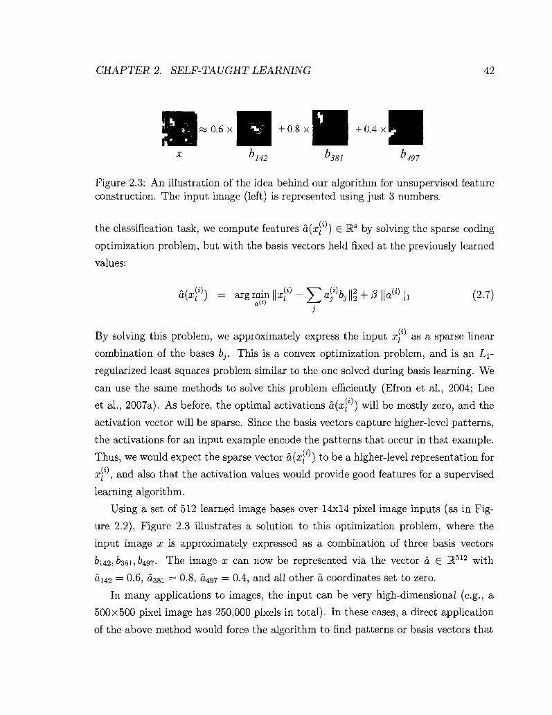
CHAPTER 2. SELF-TAUGHT LEARNING 42
S ^ H » 0 . 6 x ^ ^ 9 + 0 . 8 x l ^ H +0.4x
x b142 o381 u497
Figure 2.3: An illustration of the idea behind our algorithm for unsupervised feature construction. The input image (left) is represented using just 3 numbers.
the classification task, we compute features a(x\ ) G W by solving the sparse coding
optimization problem, but with the basis vectors held fixed at the previously learned
values:
a(xf]) = a r g m i n l l ^ - V a f y s + ^ l la^l l ! (2.7)
By solving this problem, we approximately express the input x\ as a sparse linear
combination of the bases bj. This is a convex optimization problem, and is an Li-
regularized least squares problem similar to the one solved during basis learning. We
can use the same methods to solve this problem efficiently (Efron et al., 2004; Lee
et al., 2007a). As before, the optimal activations a(x\ ) will be mostly zero, and the
activation vector will be sparse. Since the basis vectors capture higher-level patterns,
the activations for an input example encode the patterns that occur in that example.
Thus, we would expect the sparse vector a(xj ) to be a higher-level representation for
x\ , and also that the activation values would provide good features for a supervised
learning algorithm.
Using a set of 512 learned image bases over 14x14 pixel image inputs (as in Fig
ure 2.2), Figure 2.3 illustrates a solution to this optimization problem, where the
input image x is approximately expressed as a combination of three basis vectors
&U2, &38i, 497- The image x can now be represented via the vector a £ M512 with
142 = 0.6, S381 = 0.8, 0497 = 0.4, and all other a coordinates set to zero.
In many applications to images, the input can be very high-dimensional (e.g., a
500x500 pixel image has 250,000 pixels in total). In these direct application
of the above method would force the algorithm to find patterns or basis vectors that
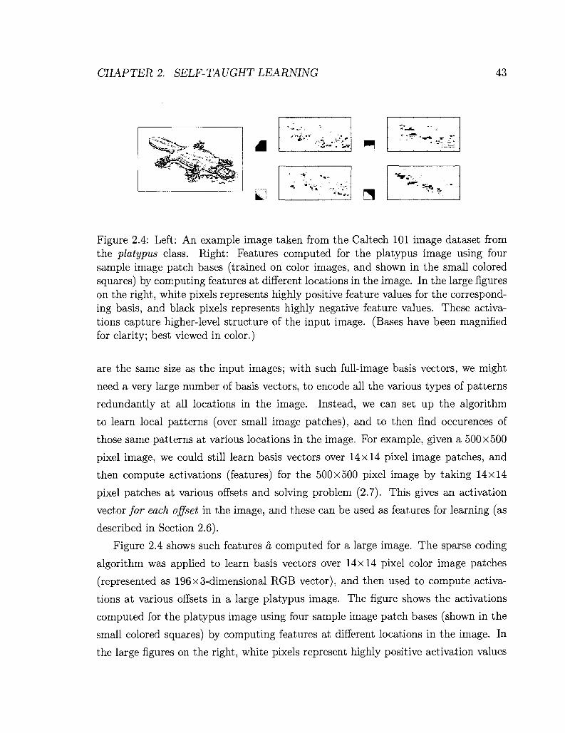
CHAPTER 2. SELF-TAUGHT LEARNING 43
Figure 2.4: Left: An example image taken from the Caltech 101 image dataset from the platypus class. Right: Features computed for the platypus image using four sample image patch bases (trained on color images, and shown in the small colored squares) by computing features at different locations in the image. In the large figures on the right, white pixels represents highly positive feature values for the corresponding basis, and black pixels represents highly negative feature values. These activations capture higher-level structure of the input image. (Bases have been magnified for clarity; best viewed in color.)
are the same size as the input images; with such full-image basis vectors, we might
need a very large number of basis vectors, to encode all the various types of patterns
redundantly at all locations in the image. Instead, we can set up the algorithm
to learn local patterns (over small image patches), and to then find occurences of
those same patterns at various locations in the image. For example, given a 500x500
pixel image, we could still learn basis vectors over 14x14 pixel image patches, and
then compute activations (features) for the 500x500 pixel image by taking 14x14
pixel patches at various offsets and solving problem (2.7). This gives an activation
vector for each offset in the image, and these can be used as features for learning (as
described in Section 2.6).
Figure 2.4 shows such features a computed for a large image. The sparse coding
algorithm was applied to learn basis vectors over 14x14 pixel color image patches
(represented as 196x3-dimensional RGB vector), and then used to compute activa
tions at various offsets in a large platypus image. The figure shows the activations
computed for the platypus image using four sample image patch bases (shown in the
small colored squares) by computing features at different locations in the image. In
the large figures on the right, white pixels represent highly positive activation values
CHAPTER 2. SELF-TAUGHT LEARNING 44
for the corresponding basis vector, and black pixels represents highly negative acti
vation values. These activations capture various types of higher-level structure of the
input image, and as we show in Section 2.6, allow us to learn a good classifier for
image categories.
These observations are not limited to images. The same method applies equally
well to other input types; the features computed on audio samples or text documents
similarly detect useful higher-level patterns in the inputs, and can be used to learn
good classifiers for audio or text categories respectively.
On all applications, we use these features as input to standard supervised clas
sification algorithms (such as SVMs). Using labeled training data, the supervised
classification algorithm learns a classifier over our activation features. To classify a
test example, we solve (2.7) to obtain feature vector a for the example, and use that as
input to the trained classifier. Algorithm 1 summarizes our algorithm for self-taught
learning.
2.5 Comparison with Related Methods
It seems that any algorithm for the self-taught learning problem must, at some ab
stract level, detect structure using the unlabeled data. Many unsupervised learning
algorithms have been devised to model different aspects of "higher-level" structure,
for example by constructing features automatically using unlabeled data (as discussed
in Chapter 1). However, their application to self-taught learning is more challenging
than might be apparent at first blush.
Principal component analysis (PCA) is among the most commonly used unsu
pervised learning algorithms. It identifies a low-dimensional subspace of maximal
variation within unlabeled data. Interestingly, the top T < n principal components
6i, b2,..., bT are a solution to an optimization problem that is cosmetically similar to
our formulation in (2.2):
minimize^ £ \ ||z!l) - £ \ afbj\\l (2.8)
s.t. &i, &2> • • • i br are orthogonal

CHAPTER 2. SELF-TAUGHT LEARNING 45
Algorithm 1 Self-taught Learning via Sparse Coding
y{m))}.
input Labeled training set for a classification task: T={(x(
i1\yM),(x\2\yW),...,(xlm\
Unlabeled data {xi, , xi , . . . , xi } Test example x.
output Predicted label for test example x. algorithm
Initialize basis vectors b randomly, s.t. ||6j|| < 1 Vj. while convergence criterion is not satisfied do
Compute activations a* by solving problem (2.4): I (») ,(0i 7.(01 mmo(i) \\Xu - Y,j a>jbj\\2 + P \\a" 'Hi
Compute basis vectors b by solving problem (2.6):
mmfe E i l l ^ - E j ^ i l l l s-t. INI < 1, Vj end while Fix the basis vectors b at the learned values.
For each labeled example x\1', compute features a(x\ ): *l (i)\ • ll (0 v* M L 112 i o ll fill I
a(xj') = argmina(i) ||x,v - ^ a) ;6j|r + /? | |aw | | i . Construct the new labeled training set:
> Basis learning
(2)> (a(x\m)),y^)} f = {(a(x{1)),yW)J(a(xJ(2)),i/
Learn a classifier C by applying a supervised learning algorithm (e.g., SVM) to the labeled training set T.
Compute features a(x) for test input x:
a(x) = argminQ \\x - J2jajbj\\2 + P ||a||i-return prediction of the classifier C on the features a(x).
> Construct features
> Prediction

CHAPTER 2. SELF-TAUGHT LEARNING 46
The basis vectors are constrained to be orthogonal to each other—the resulting for
mulation has the useful properties that the subspace spanned by the basis vectors
b\,b2, •.. ,br is optimal among all T-dimensional subspaces (in terms of Euclidean
distance of the points from the subspace), and that there is no redundancy in the
activations as they capture orthogonal basis vector directions (technically, the acti
vations corresponding to any two basis vectors, a ; i and aj2, are uncorrelated with
each other in the training data {x\l })• When formulated in this way, PCA differs
from our sparse coding formulation in two ways: PCA does not enforce sparsity of
the activations, and PCA constrains basis vectors to be orthogonal (or orthonormal
if the basis vectors are also normalized to have unit norm).
PCA is convenient because the above optimization problem can be solved ef
ficiently using standard numerical software; the absence of an Li-sparsity penalty
term leads to a solution that can be computed simply via an eigenvector decomposi
tion, without the need for an iterative alternating minimization procedure. Further,
given basis vector bj, the corresponding features a? can be computed easily because
of the orthogonality constraint, and are simply a? = bjxu (independent of the basis
vectors other than bj).
When compared with sparse coding as a method for constructing self-taught learn
ing features, PCA has two limitations. First, PCA results in linear feature extraction,
in that the features a* are simply a linear function a* = bjxu of the input xj, . This
appears to be a severe restriction. As an example of a nonlinear but useful feature
for images, consider the phenomenon called end-stopping (which is known to occur
in biological visual perception (Sceniak et al., 2001)) in which a feature is maximally
activated by edges of only a specific orientation and length; increasing the length
of the edge further significantly decreases the feature's activation. A linear response
model cannot exhibit end-stopping. Second, since PCA assumes the bases bj to be or
thogonal, the number of PCA features cannot be greater than the dimension n of the
input. Sparse coding does not have either of these limitations. Its features a(x) are an
inherently nonlinear function of the input x, as they are computed by solving an op
timization problem in Equation (2.7), where the Li-term provides a strong incentive
to set many features exactly to zero. In fact, we have shown that sparse coding can

CHAPTER 2. SELF-TAUGHT LEARNING 47
exhibit end-stopping behavior (Lee et al., 2007a). Note also that even though sparse
coding attempts to express x as a linear combination of the bases bj, the optimization
problem (2.7) results in the activations a(x) being a nonlinear function of x. Further,
sparse coding can use more basis vectors/features than the input dimension n. By
learning a large number of basis vectors but using only a small number of them for
any particular input, sparse coding gives a higher-level representation in terms of the
many possible "basic patterns," such as edges, that may appear in an input.
As we noted earlier, sparse coding differs from PCA in two major ways: it adds
an Li-penalty enforcing sparsity of activations, and it replaces the orthogonality con
straint on the basis vectors by a much weaker normalization constraint. PCA can
be modified in various ways to make it more similar to sparse coding. The simplest
way would be to add in the Li-penalty term to the PCA formulation (2.8-2.9), thus
leading to a sparse PCA formulation such as the following:1
minimize^ £ , ||a#> - £ ^ 5 % I I 2 + 0 £ « \\a^% (2.9)
s.t. bi, &2, • • •, &T a r e orthogonal
This sparse PCA formulation can be solved efficiently using the alternating minimiza
tion algorithm used for sparse coding, because the additional orthogonality constraint
simplifies each of the minimization steps: (i) We can optimize the activations a while
keeping basis vectors b by a linear operation, as for PCA, followed by an additional
thresholding step that pulls every individual activation value a,- closer to zero by
resetting it to max(0, a,- — sign (a,) • /?). Intuitively, the effect of the Li-term acts
individually on the activation values, and we do not need to explicitly solve an opti
mization problem jointly over all the activation values, because the basis vectors are
orthogonal and act on orthogonal input subspaces. (ii) We can optimize the basis
vectors b while keeping the activations a fixed via a singular value decomposition, as 1Note that simply relaxing the orthogonality constraint in the PCA formulation, without adding
the Li-penalty term, would not help, as one of the optimal solutions for such a formulation would consist of orthogonal basis vectors. In other words, without a sparsity constraint on activations, there is no incentive against making any two basis vectors orthogonal to each other, as long as the subspace spanned by the basis vectors does not change.

CHAPTER 2. SELF-TAUGHT LEARNING 48
in PCA.
Unfortunately, this sparse PCA formulation also did not perform well on self-
taught learning problems in our experiments. One significant drawback this formula
tion shares with PCA is that the number of basis vectors is still limited by the input
dimension, due to the requirement that basis vectors be orthogonal to each other. In
particular, the number of basis vectors must still be less than the input dimension (as
in the case of PCA), and overcomplete basis vectors cannot be learned. In practice,
input data from many domains often lies close to a low-dimensional subspace (of lower
dimension that the input dimension n), and this further exacerbates the problem—if
the data lies close to a 20-dimensional subspace, 20 basis vectors are sufficient to span
the subspace, and there is little extra information to learn further basis vectors (even
considering the Li-penalty term to encourage sparsity).
The differences between sparse coding, PCA, and the above sparse PCA for
mulation can be illustrated through a sample of the basis vectors learnt by them.
Figure 2.5(a)-(c) shows 100 basis vectors obtained when the respective optimization
problems were solved with 100,000 input images, each representing a 14x14 pixel
image extracted at random from unlabeled grayscale images of natural scenes.2 Each
input x$ e M196 lies in a 196-dimensional space of pixel intensities, but even 100
principal components are sufficient to explain over 97% of the variance in the input
data, and consequently, it appears hard to learn any more than 100 useful basis vec
tors (or features) by using PCA. In Figure 2.5(a), PCA basis vectors are ordered top
to bottom by decreasing variance of the input data along the basis vector. The dif
ferences between PCA and sparse coding have been well-documented—sparse coding
learns basis vectors that are oriented and spatially localized, modeling various types
of edges, but PCA does not learn such basis vectors. (Olshausen & Field, 1996a) The
sparse PCA formulation in Figure 2.5(b) learns some edge-like basis vectors, but as
expected, cannot learn more than a few such vectors. The basis vectors are ordered
from top to bottom by decreasing fraction of input examples that have a nonzero
2Other details: For sparse coding and sparse PCA, we used the same sparsity penalty parameter /? = 0.7, which lead to 7% nonzero activations per input example on average. Following standard preprocessing, we centered the data by subtracting the mean pixel intensity for each pixel in the dataset.

CHAPTER 2. SELF-TAUGHT LEARNING 49
activation value for the basis vector, and the basis vectors in the bottom half are
activated only for a small fraction of the input examples. For example, the bottom
20 basis vectors were active for less than 1% of the input examples.
By not imposing the orthogonality constraint, sparse coding can learn a much
larger number of usable basis vectors. Each sparse coding basis vectors displayed
in Figure 2.5(c) had a nonzero activation for between 6% to 9% of the examples.
(The basis vectors are ordered by decreasing fraction of input examples that have a
nonzero activation value for the basis vector.) Sparse coding can be applied to learn
more basis vectors, and Figure 2.5(d) shows an example with 400 basis vectors. Even
in this case, all basis vectors had nonzero activations for between 2% to 4% of the
examples (the average fraction of activations per example in this case was 3%).
There are other modifications of PCA that enforce sparsity by formulating the
problem differently. For example, Zou et al. (2004) use an "elastic net penalty" in
stead of our Li-penalty, but still constrain the basis vectors to be orthogonal. A differ
ent method consists of finding a matrix factorization for the input matrix X ~ UV,
for matrices U and V, by additionally constraining U and V to be sparse (Srebro
& Jaakkola, 2001), or by placing linear constraints on the entries of U and V vari
ables (Lee & Seung, 1997). Some of these methods can produce basis vectors that look
similar to basis vectors learned by sparse coding, in that they learn edge-like features
on natural images (e.g., see Lee & Seung, 1997), but they differ in the details of their
formulation, and in the way that a new input is mapped to activations (features). Lee
& Seung (1997) show that their factorization method can be used for classification of
handwritten digits, but the basis vectors were learned on the labeled training data
itself (by learning a separate set of basis vectors per label class). Variations of these
methods might be applicable to self-taught learning problems, but we are not aware
of any previous applications.
A different modification of PCA can also address the concern that PCA learns a
linear mapping a^ = bjxu from input x£ to features <r-'. Kernel dimensionality
reduction algorithms such as kernel PCA (Mika et al., 1999) implicitly operate linearly
in a potentially high-dimensional space, but due to the implicit mapping to a high-
dimensional space, they can behave very nonlinearly in the input space. (For example,

CHAPTER 2. SELF-TAUGHT LEARNING 50
%,* v # Fir.* #
i s *
n & P
M J fr&
53§5n #« '***
V
T*&\ j % i «y
4 11 f i
s * ? ^ .•»JV fcja
n!?, H-» -a t,
V«
W F ^ <*i# %
^u ^P*«. ""* inr* * M r
1.1* 45 m • ^ • V . 4
fa •Si !*«#£
HI ^ nffiTt
I Ml i l l
III MM SS! M'"JL
Jlj ' P!TT
-AT iffl es I? [jVtf «
I I I
K3K H Isi&P rmra
11 <t i
£ M =a*
TW1 h i " * m -fVivt r.r.n I
U fmrt If •i-sJiW M | ~ a ~ ^
111J3JI •ct:i if '}' :S. 8
fa) PCA
IT W % r xj
I i
1* iM M 5H ^ a *
T ' ^ • ^ 1 4£?&
, K-- ME W n sf -^
^ K 5^fv-' w n &^ w LJ~ *&A C&1 .'-V M R l • •
•« . U S 1 * 7 ^ ^ S
Mi g3£ # * i'-l I
tt'»M •*:>*.- Li : * \ < * * " • • '
.Ms (b) Our sparse PCA formulation
^ P
j * .
"\
J> 1
1
/
* . '
'l;
y \
m —
_ : ?
ft*
t 4
1 ' l
J*
—!»^
^
"" S
^^tf*1 ' ' '
,-*"*
>? ^
• *
. >
>s k.
";i
1 f
Al
^
^-flWP
* f c . 1
\
^
/
H
* / %.
* ' M
^
' / 'S.'
\<
' •
%
\
k i
i V
li
\
^
V i
1-7 *
\
! i
i
- »
V .,<
-
i f^
w
/
^
, ^ -
%
^ • ^
£$ : l (
1 \
(c) Sparse coding with 100 basis vectors
1
•? 1
).* -Iff1
•w
V
*«
^ j
i
^ —
V
j / / ' */
f 1#
-
y ^ p
i *
% « •
K.
i « * •«<
ji"
h %
"
flf "
r -•r
• •
'';
*>
» ' ,
:'* . *•
' ' «» ^<
*a
t . . .
* / • ^
w [« '
*C
^
'•"4
^ j / H
i #'
K "S
^ *••
''• i^ i
^ • j *
..-
>?•
> N
"l
A
*
* T
>-'
• ' \
? if
*
\ A
<ft i
•-i l
.1
/ -V
« ' • < •
L
\ l*-
V
* . ' • •
- * HM4
•f &
•* • -'l
i l i
\ ."
p \
-1
$ .1
v'. , " i *
• X
*> "'f
# ^
> T
P \
ill
I.
*
V
# r
•t
f 'i
*
t-
^
,-i i '
'li *-.'*
"»-. *•
t
J*
•s "T
1
^ fv
N
- • «
„,
— K
< /
I s f?
'*
i ' '
.si
<*•
- i
.i -< •».
'/ *•*
«*•
'-# V; V' r A
! • :
^ ^ ' • 1
S.
,,«
•r i »v
r
>< ' i
\ fr >'
<?• .11
. -
1
•^ 1 ^ ' * *.
^ K 'f;
^ ••
•V «. *
* • "
"*
^ >
<•-
^ ' • «
/ 1
i
j r "3
x t-IL . •
.!«;
ar
t
f ^
—'-i
'«>
- > • ' *
*s. K
I' f
i
\ •
» •n
'I
| Vw
St. w;
^
»i
\
n«
^ / «i"
^ # •*. 1
•J»
w p
r •s
f
> *
• \
* i
$ i . i i •
»-
• • >
• "
V
' * * ir.'
«
^
4k.
/
.7 *
s
t
• « •
»/
*>• V %
— *r-
' /
r 11
•i
\ '' [»
" / V
>S
. '* *s
' '%
\ 4 *
\ .4
k 1
SL *
r*;
«! V
A y
/ j .
»'
v
(d) Sparse coding with 400 basis vectors
Figure 2.5: Basis vectors learned by PCA, PCA with sparsity, and sparse coding on unlabeled input images. A single square box in each figure denotes a basis vector.
CHAPTER 2. SELF-TAUGHT LEARNING 51
a linear function in the space of "all-pairs" features with elements XjxXj2, for any two
input dimensions j \ and j'2, is equivalent to a quadratic function in the space of the
original feature space x.) This removes the restriction to linear mappings in PC A,
while still allowing an efficient solution. But kernel PCA still requires a "kernel
function" that captures a useful similarity metric over the input data (we give a brief
introduction to kernel functions in 2.7.2), and such a kernel function can be hard to
hand-design or learn from unlabeled data.
The independent components analysis (ICA) algorithm attempts to find basis
vectors bj such that the activation a? = bjxu is maximally independent from the
activations for other basis vectors. (Bell & Sejnowski, 1995) By encouraging indepen
dence of the activations (features), ICA produces a representation that has very low
redundancy. ICA is also known to learn basis vectors similar to sparse coding basis
vectors, and has been widely studied in computational neuroscience. (van Hateren &
van der Schaaf, 1998) Unfortunately, as a self-taught learning method for learning
features, ICA did not work well in our experiments. One reason for this could be
that ICA still defines a linear mapping from inputs Xu to features a- . It is possible
that some nonlinear ICA methods (Hyvarinen & Pajunen, 1999) can be applied to
self-taught learning problems.
Nonnegative matrix factorization (NMF) is a matrix factorization method that
represents the input data matrix X approximately as a product of two matrices U and
V with only nonnegative elements: X ~ UV. Nonnegative matrix factorization has
been shown to learn "parts" of images automatically from data. (Lee & Seung, 1999)
However, we are not familiar with previous applications to problems where the parts
are learned on a very different, unlabeled source of data, and then applied to represent
a target labeled dataset. Some of the ideas in nonnegative matrix factorization might
be applicable to self-taught learning problems.
In Chapter 1, we discussed the vector quantization method (VQ) for transforming
input vectors Xu (or hand-designed features of Xu) to a single "codeword," where the
codewords are themselves learnt on the unlabeled data. In comparison with sparse
coding, which represents each input vector using a few patterns (basis vectors), VQ
represents every input vector by using exactly one pattern (codeword). When VQ is

CHAPTER 2. SELF-TAUGHT LEARNING 52
used with the Euclidean distance measure to map inputs to codewords, this link can
be further formalized: with the k-means clustering algorithm used for learning the
codewords, VQ is mathematically identical to our sparse coding formulation, with
(3 set to a high value that guarantees exactly one nonzero activation, and with the
activations only allowed to take the values 0 or l.3 The typical application of VQ
thus appears more restrictive than sparse coding, and in Section 2.6.3 we demonstrate
that sparse coding works better than a VQ method that is used widely in computer
vision applications.
Methods based on VQ have been further customized to certain applications such
as computer vision (Grauman & Darrell, 2007) and speech processing (Rabiner &
Juang, 1993), though the codewords are usually learnt on the labeled training data
itself. Nevertheless, it is plausible that such methods can be applied to self-taught
learning problems as well.
In the semi-supervised learning setting, several authors have previously constructed
features using labeled or unlabeled data from the same domain as the labeled data
(e.g., see Chapter 1 for a detailed discussion of several such methods). A recent ex
ample is provided by the influential work of Hinton & Salakhutdinov (2006),, in which
the authors train a multilayer neural network to learn features for handwritten digit
images. They obtain striking results by using handwritten digit images themselves
to construct features. In contrast, self-taught learning poses a harder problem, and
requires that the structure learned from unlabeled data from a different domain (such
as handwritten digit images) be "useful" for representing data (such as handwritten
English character images) from the classification task.
Several existing methods for unsupervised and semi-supervised learning can be
applied to self-taught learning, though many of them do not lead to good performance.
For example, consider the task of classifying images of English characters ("a"—"z"),
using unlabeled images of digits ("0"—"9"). For such a task, manifold learning
algorithms such as ISOMAP (Tenenbaum et al., 2000) or LLE (Roweis & Saul, 2000)
can learn a low-dimensional manifold using the unlabeled data (digits); however, these
3 Technically, /? must be set to a separate value per input example to ensure that only one activation is nonzero.

CHAPTER 2. SELF-TAUGHT LEARNING 53
manifold representations do not generalize straightforwardly to the labeled inputs
(English characters) that are dissimilar to any single unlabeled input (digit). As
discussed in Chapter 1, neural network models such as autoencoders can also be
applied to self-taught learning problems. To the best of our knowledge, they have
only been applied to learning features from the same domain as the labeled data, and
not to self-taught learning problems.
2.6 Experiments
We apply our algorithm to several self-taught learning tasks shown in Table 2.1. Note
that the unlabeled data in each case cannot be assigned the labels from the labeled
task. For each application, the raw input examples x were represented in a standard
way with almost no hand-engineered preprocessing: raw pixel intensities for images,
the frequency spectrogram for audio, and the bag-of-words (vector) representation
for text documents.
2.6.1 Implementation details
For computational reasons, the unlabeled data was preprocessed by applying PCA to
reduce its dimension;4 the sparse coding basis learning algorithm was then applied in
the resulting principal component space. We note that reasonable basis vectors can
often be learned even using a smooth approximation such as ^(a) = ( ^ . J a1 + e)
to the Li-norm sparsity penalty \I/(a) = ||a||i; the smooth approximation leads to a
differentiable objective function, and a much faster sparse coding algorithm. However,
such approximations do not produce sparse features, and in our experiments, we found
that classification performance is significantly worse if such approximations are used
to compute a(x\ ).5
4We picked the number of principal components to preserve approximately 96% of the unlabeled data variance. This allowed us to apply sparse coding over a lower-dimensional input space, while preserving almost all of the input information.
5There is recent work showing that a smooth sparsity penalty based on the KL divergence measure can also work well for self-taught learning problems (Bradley & Bagnell, 2008).

Dom
ain
Imag
e cl
assi
fica
tion
Han
dwri
tten
ch
arac
ter
reco
gnit
ion
Font
ch
arac
ter
reco
gnit
ion
Song
ge
nre
clas
sifi
catio
n
Web
page
cl
assi
fica
tion
Use
Net
ar
ticl
e cl
assi
fica
tion
Unl
abel
ed d
ata
10
imag
es
of
outd
oor
scen
es
Han
dwri
tten
di
gits
("
0"-"
9")
(LeC
un
k C
orte
s, 1
998)
H
andw
ritt
en
Eng
lish
ch
arac
ters
("
a"-
"z")
(T
aska
r, 2
004)
So
ng
snip
pets
fr
om
10
genr
es
(Mag
-na
tune
da
tase
t:
htt
p:/
/mag
nat
un
e.co
m
100,
000
new
s ar
ticl
es
from
th
e R
eute
rs
cor
pus
(Ros
e et
al,
200
2)
100,
000
new
s ar
ticl
es
from
th
e R
eute
rs
cor
pus
(Ros
e et
al,
200
2)
Lab
eled
dat
a C
alte
chlO
l im
age
clas
si
fica
tion
data
set
(Fei
-Fei
et
al.,
200
4)
Han
dwri
tten
E
ngl
ish
char
acte
rs
("a"
-"z
") (
Tas
kar,
200
4)
Font
ch
arac
ter
imag
es
("a'
7"A
"-"z
'7"Z
") o
bta
ined
usi
ng L
inux
fon
ts
Song
sn
ippe
ts
from
7
diff
eren
t ge
nres
(M
agna
tune
da
tase
t:
1 h
ttp
://m
agn
atu
ne.
com
) C
ateg
oriz
ed
web
-pa
ges
from
th
e D
MO
Z
hier
arch
y (h
ttp:
//w
ww
.dm
oz.o
rg)
Cat
egor
ized
U
seN
et
post
s fr
om t
he "
SRA
A"
data
set
(McC
allu
m,
2000
)
Cla
sses
10
1
26
26
7 2 2
Raw
fea
ture
s In
tens
itie
s in
14
x14
pixe
l pa
tch
Inte
nsit
ies
in
28x2
8 pi
xel
char
acte
r/di
git
imag
e In
tens
itie
s in
28
x28
pixe
l ch
arac
ter
imag
e
Log
-fre
quen
cy
spec
tr
ogra
m
over
50
ms
tim
e w
indo
ws
Bag
-of-
wor
ds w
ith
500
wor
d vo
cabu
lary
Bag
-of-
wor
ds w
ith
377
wor
d vo
cabu
lary
fen
Tab
le 2
.1:
Det
ails
of
self
-tau
ght
lear
ning
app
lica
tion
s ev
alua
ted
in t
he e
xper
imen
ts.
4^

CHAPTER 2. SELF-TAUGHT LEARNING 55
Once the basis vectors were learned on unlabeled data, they were used to construct
features for each input from the supervised classification task.6 The basis vectors
were trained on the unlabeled data source, and are thus optimized to represent those
examples with sparse activations (using very few basis vectors per input example).
When the basis vectors are applied to computing activations for labeled data, to
which the basis vectors were not tuned in advance, the same value of sparsity penalty
(3 can lead to a higher number of nonzero activation values. Since the labeled and
unlabeled data can sometimes lead to very different numbers of non-zero coefficients
dj, in our experiments (5 was also recalibrated prior to computing the labeled data's
representations a(xf'). We recommend that j3 used for computing this labeled data
representation be picked by cross-validation on the labeled data.
For each such task, we report the result from the better of two standard, off-the-
shelf supervised learning algorithms: a support vector machine (SVM) and Gaussian
discriminant analysis (GDA). We used completely standard, off-the-shelf SVM and
GDA classifiers that were not customized to the sparse coding features in any way,
to demonstrate the utility of the learned features. A classifier specifically customized
to sparse coding features is described in Section 2.7.
Partly for scaling and computational reasons, an additional feature aggregation
step was applied to the image and audio classification tasks (since a single image is
several times larger than the individual/small image patch bases that can be learned
tractably by sparse coding). We aggregated features for large input images by ex
tracting features for small image windows ("patches") in different locations in the
large image, and then aggregating the features per-basis by taking the feature value
with the maximum absolute value. The aggregation procedure effectively looks for
the "strongest" occurrence of each basis pattern within the image. (Even better
performance is obtained by aggregating features over a KxK grid of regions, thus
looking for strong activations separately in different parts of the large image; see Ta
ble 2.2.) These region-wise aggregated features were used as input to the classification
6If PCA was used to reduce the dimensionality of inputs at basis learning time, by transforming input vector Xu to the vector Pxu for a matrix P containing the PCA parameters, the same PCA transform was applied on the labeled data as well to transform input x\ to Px\1'.

CHAPTER 2. SELF-TAUGHT LEARNING 56
algorithms (SVM or GDA). Features for audio snippets were similarly aggregated by-
computing the maximum activation per basis vector over 50ms time windows in the
snippet.
In the previous section, we compared our sparse coding formulation with many
other methods for learning from unlabeled data. In this section, we compare our self-
taught learning algorithm against two baselines, also trained with an SVM or GDA:
using the raw inputs themselves as features, and using principal component projec
tions as features, where the principal components were computed on the unlabeled
data (as described in Section 2.5). In the PCA results presented in this paper, the
number of principal components used was always fixed at the number of principal
components used for preprocessing the raw input before applying sparse coding. This
control experiment allows us to evaluate the effects of PCA preprocessing and the
later sparse coding step separately, but should therefore not be treated as a direct
evaluation of PCA as a self-taught learning algorithm (where the number of principal
components could then also be varied). There is a vast variety of methods that can be
used for "learning from unlabeled data," though we are not aware of previous appli
cations of such methods to general self-taught learning problems. In Section 2.6.3, we
delve deeper into the computer vision domain, and compare our results more broadly
with previous techniques that use various kinds of unlabeled data.
2.6.2 Results
Tables 2.2-2.6 report the results for various domains. Sparse coding features, possibly
in combination with raw features, significantly outperform the raw features alone as
well as PCA features on most of the domains.
On the 101-way Caltech 101 image classification task with 15 training images
per class (Table 2.2), sparse coding features achieve a test accuracy of 46.6%. In
comparison, the first published supervised learning algorithm for this dataset achieved
only 16% test accuracy even with computer vision specific features (instead of raw
pixel intensities). Further, at the time we ran our experiments, our results were
competitive with the best reported results on the dataset (Fei-Fei et al., 2004; Berg

CHAPTER 2. SELF-TAUGHT LEARNING 57
Features
PCA Sparse coding Published base
Number of regions 1 4 9 16
20.1% 30.6% 36.8% 37.0% 30.8% 40.9% 46.0% 46.6%
line (Fei-Fei et al., 2004) 16%
Table 2.2: Classification accuracy on the Caltech 101 image classification dataset. For PCA and sparse coding results, each image was split into the specified number of regions, and features were aggregated within each region by taking the maximum absolute value.
et al., 2005; Holub et al., 2005; Serre et al., 2005). This is quite remarkable, since those
other results required extensively researched computer vision specific techniques, and
often used carefully hand-designed features or classifiers, while our method was based
on an almost completely unsupervised algorithm with almost no explicit computer
vision specific methods or human hand-engineering of features.7
Figure 2.6 shows example input images from the three character datasets, and
some of the learned basis vectors. The learned basis vectors appear to represent
"pen strokes." In Table 2.3, it is thus not surprising that sparse coding is able to
use basis vectors ("strokes") learned on digits to significantly improve performance
on handwritten characters—it allows the supervised learning algorithm to "see" the
characters as comprising strokes, rather than as comprising pixels.
For audio classification, our algorithm outperforms the raw (spectral) features
(Table 2.4).8 In Chapter 4, we present a more sophisticated sparse coding algorithm
for audio classification, and show that sparse coding methods outperform spectral
features as well as some hand-engineered music/speech specific features.
When applied to text, sparse coding discovers word relations that might be useful
7 Since the time we ran our experiments, other researchers have reported even better results using highly specialized computer vision algorithms (Zhang et al., 2006: 59.1%; Lazebnik et al., 2006: 56.4%). (Zhang et al., 2006; Lazebnik et al., 2006) Some of the computer vision specific ideas in these methods, such as Lazebnik's spatial pyramid kernel for aggregating local image features into global predictions, can also be applied directly to sparse coding features. This would give a computer vision specific self-taught learning method that might work better on this image classification dataset.
8Details: We learned bases over songs from 10 genres, and used these bases to construct features for a music genre classification over songs from 7 different genres (with different artists, and possibly different instruments). Each training example comprised a labeled 50ms song snippet; each test example was a 1 second song snippet.

CHAPTER 2. SELF-TAUGHT LEARNING 58
t>
„ _
*
*
t?
/
- t 3
» •
/
k
£*
fr
*
D
. 3
fr *
# "»
- 9 "
<*-
*
c -
*
i 1
•e- t
4>
li
i
9
«_
ff
m
i tS g
^
K 3
m
(a) (b)
Figure 2.6: (a) Example images from the handwritten digit dataset (top), the handwritten character dataset (middle) and the font character dataset (bottom), (b) Example sparse coding bases learned on handwritten digits.
Digits —> English handwritten characters Training set size Raw PCA Sparse coding
100 39.8% 25.3% 39.7% 500 54.8% 54.8% 58.5% 1000 1 61.9% 64.5% 65.3%
Handwritten characters —• Font characters Training set size Raw PCA Sparse coding
100 8 2% KWo 7.0% (9.2%) 500 17.9% 14.5% 16.6% (20.2%) 1000 1 25.6% 23.7% 23.2% (28.3%)
Table 2.3: Top: Classification accuracy on 26-way handwritten English character classification, using basis vectors trained on handwritten digits. Bottom: Classification accuracy on 26-way English font character classification, using basis vectors trained on English handwritten characters. The numbers in parentheses denote the accuracy using raw and sparse coding features together. Here, sparse coding features alone do not perform as well as the raw features, but perform significantly better when used in combination with the raw features.

CHAPTER 2. SELF-TAUGHT LEARNING 59
Training set size 100 1000 5000
Raw PCA Sparse coding 28.3% 28.6% 44.0% 34.0% 26.3% 45.5% 38.1% 38.1% 44.3%
Table 2.4: Classification accuracy on 7-way music genre classification, using basis vectors trained on songs from 10 different genres.
Design design, company, product, work, market Business car, sale, vehicle, motor, market, import vaccine infect, report, virus, hiv, decline, product movie share, disney, abc, release, office, movie, pay
Table 2.5: Text basis vectors learned on 100,000 Reuters newswire documents. Top: Each row represents the basis vector most active on average for documents with the class label at the left. For each basis vector, the words corresponding to the largest magnitude elements are displayed. Bottom: Each row represents the basis vector that contains the largest magnitude element for the word at the left. The words corresponding to other large magnitude elements are displayed.
for classification (Table 2.5). The performance improvement over raw features is
small (Table 2.6).9 This might be because the bag-of-words representation of text
documents is already sparse, unlike the raw inputs for the other applications, and
because the bag-of-words representation contains either binary (0/1) or integer-valued
features, which are poorly approximated by the quadratic term in the sparse coding
objective function. In Chapter 4, we elaborate further on this problem, and show
that a more general sparse coding model works even better on text classification;
that model also outperforms Latent Dirichlet Allocation (Blei et al., 2003), a method
that is widely used for unsupervised learning with text documents.
We envision self-taught learning as being most useful when labeled data is scarce.
Table 2.7 shows that with small amounts of labeled data, classification performance
deteriorates significantly when the basis vectors (in sparse coding) or principal com
ponents (in PCA) are learned on the labeled data itself, instead of on large amounts of
9Details: Basis vectors were learned on 100,000 news articles from the Reuters corpus (Rose et al., 2002), and then evaluated on 30 binary webpage category classification tasks, and on 2 binary UseNet article classification tasks. PCA applied to text documents is commonly referred to as latent semantic analysis. (Deerwester et al., 1990)

CHAPTER 2. SELF-TAUGHT LEARNING 60
Reuters news —> Webpages Training set size Raw PCA Sparse coding
4 10 20
Reuters Training set size
4 10
62.8% 63.3% 64.3% 73.0% 72.9% 75.9% 79.9% 78.6% 80.4%
news —» UseNet articles Raw PCA Sparse coding
61.3% 60.7% 63.8% 69.8% 64.6% 68.7%
Table 2.6: Classification accuracy on webpage classification (top) and UseNet article classification (bottom), using bases trained on Reuters news articles.
additional unlabeled data.10 This demonstrates that our method is in fact using the
unlabeled data, and cannot simply be applied successfully to a supervised learning
problem with no unlabeled data. As more and more labeled data becomes available,
the performance of sparse coding trained on labeled data approaches (and presumably
will ultimately exceed) that of sparse coding trained on unlabeled data.
2.6.3 Other methods of using unlabeled data
To the best of our knowledge, the self-taught learning framework places significantly
fewer restrictions than previous formalisms for using unlabeled data for a supervised
learning task. However, there are many published algorithms in the literature that use
some form of "weakly related" unlabeled data for a specific application, and as such,
those algorithms can be applied to self-taught learning problems. As a case study,
we consider experimental results for the CaltechlOl image classification dataset, as
it is a standard dataset with a significant body of published results, and compare
the results obtained by our self-taught learning algorithm with other data-driven
methods. For comparison, our sparse coding method achieves an accuracy of 46.6%
on the CaltechlOl dataset with 101 image classes and 15 training examples per class.
A widely used method in computer vision is based on the vector quantization or
"bag-of-visual-words" technique (see Section 1.6.2 for an introduction). Briefly, this
10For the sake of simplicity, we performed this comparison only for the domains that the basic sparse coding algorithm applies to, and that do not require the extra feature aggregation step.

CHAPTER 2. SELF-TAUGHT LEARNING 61
Domain
Handwritten characters
Font characters
Webpages
UseNet
Training set size
100 500 1000 5000 100 500 1000
4 10 20 4 10
Unlabeled SC
39.7% 58.5% 65.3% 73.1% 7.0%
16.6% 23.2% 64.3% 75.9% 80.4% 63.8% 68.7%
Labeled PCA SC 36.2% 50.4% 62.5% 73.5% 5.2% 11.7% 19.0% 55.9% 57.0% 62.9% 60.5% 67.9%
31.4% 50.8% 61.3% 73.0% 5.1% 14.7% 22.3% 53.6% 54.8% 60.5% 50.9% 60.8%
Table 2.7: Accuracy on the self-taught learning tasks when sparse coding bases are learned on unlabeled data (third column), or when principal components/sparse coding bases are learned on the labeled training set (fourth/fifth column). Since Tables 2.2-2.6 already show the results for PCA trained on unlabeled data, we omit those results from this table. The performance trends are qualitatively preserved even when raw features are appended to the sparse coding features.
technique uses a large number of example images to learn a set of local patterns, also
called codewords or "visual words," and then uses a single pattern to describe any
local image feature. Grauman & Darrell (2007) performed an extensive study of such
bag-of-visual-words methods. They used the hand-designed SIFT features as local
image features (Lowe, 1999), and preprocessed the features by applying a principal
component analysis (PCA) transform to give the so-called "PCA-SIFT" features (Ke
& Sukthankar, 2004). These PCA-SIFT features have been shown to be comparable
to, or outperform, various other types of local features for image classification (Miko-
lajczyk & Schmid, 2005), including a large number of local descriptors developed over
the past decade in computer vision research.11 Given the extensive comparisons with
11The descriptors compared by Mikolajczyk & Schmid included gradient location and orientation histograms or GLOH (Mikolajczyk & Schmid, 2005), shape context (Belongie et al., 2002), sift (Lowe, 1999), spin images (laz, 2005), steerable filters (Freeman & Adelson, 1991), differential invariants (Koenderink & van Doom, 1987), complex filters (Schaffalitzky & Zisserman, 2002), moment invariants (Gool et al., 1996), and cross-correlation of sampled pixel values.

CHAPTER 2. SELF-TAUGHT LEARNING 62
other feature types, we are not aware of a better local feature type that could have
been used instead of the PCA-SIFT features. In their study, Grauman & Darrell
learnt the codewords on labeled training data itself (and not on unrelated unlabeled
data); they also extensively tuned various parameters in the classification algorithm,
including the number of patterns (codewords), the distance metric used to map to
a local PCA-SIFT feature to the closest pattern, and also the SVM classification
hyperparameters. Even with all these customizations, the best results reported us
ing a standard support vector machine classifier were around 38% accuracy on the
CaltechlOl dataset, which is much lower than the 46.6% obtained by our method.
In addition, Grauman & Darrell note that the bag-of-visual-word approach's accu
racy was fairly sensitive to the exact parameter settings; in comparison our algorithm
requires little parameter tuning.12
The above results with bag-of-visual-words were obtained when codewords were
trained by clustering the labeled training data itself. We would expect that the
results might be comparable or worse if the codewords are trained on other unlabeled
images, as the trained codewords would be optimized for representing features from
those unlabeled images. We confirmed this in the following control experiment. We
trained codewords in two different ways: either using the labeled training set, or using
a set of unlabeled images different from the labeled training set. We found that the
final results did not change significantly in these two experiments. Combined with
Grauman & DarreU's study, this indicates that using standard supervised learning
classifiers, the typical bag-of-visual-words method does not perform as well as our
sparse coding method on self-taught learning applied to image classification. 12In their paper, Grauman & Darrell use the study reported here as a baseline. They design an
ingenious method called the pyramid match kernel for matching local features from one image with local features from another image. Such a matching method does not penalize for the presence of extra local features, and is thus more robust to clutter, changing backgrounds or occlusions. With this pyramid match kernel, Grauman & Darrell obtain 50% accuracy for this task which is better than the 46.6% accuracy we report here. We note that a similar pyramid match kernel can be applied to the sparse coding features as well, replacing our simplistic grid-wise-maximum feature aggregation procedure with a more sophisticated matching algorithm. In any case, we find it remarkable that our algorithm achieves an accuracy of 46.6% even though it is almost completely unsupervised, uses only unlabeled data to train the representation (unlike the codewords learnt in typical bag-of-visual-words applications), uses almost no hand-designed features, and required almost no computer vision specific tuning.
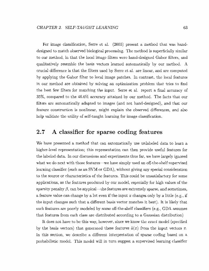
CHAPTER 2. SELF-TAUGHT LEARNING 63
For image classification, Serre et al. (2005) present a method that was hand-
designed to match observed biological processing. The method is superficially similar
to our method, in that the local image filters were hand-designed Gabor filters, and
qualitatively resemble the basis vectors learned automatically by our method. A
crucial difference is that the filters used by Serre et al. are linear, and are computed
by applying the Gabor filter to local image patches. In contrast, the local features
in our method are obtained by solving an optimization problem that tries to find
the best few filters for matching the input. Serre et al. report a final accuracy of
35%, compared to the 46.6% accuracy attained by our method. The facts that our
filters are automatically adapted to images (and not hand-designed), and that our
feature construction is nonlinear, might explain the observed differences, and also
help validate the utility of self-taught learning for image classification.
2.7 A classifier for sparse coding features
We have presented a method that can automatically use unlabeled data to learn a
higher-level representation; this representation can then provide useful features for
the labeled data. In our discussions and experiments thus far, we have largely ignored
what we do next with those features—we have simply used an off-the-shelf supervised
learning classifier (such as an SVM or GDA), without giving any special consideration
to the source or characteristics of the features. This could be unsatisfactory for some
applications, as the features produced by our model, especially for high values of the
sparsity penalty /3, can be atypical—the features are extremely sparse, and sometimes,
a feature value can change by a lot even if the input x changes only by a little (e.g., if
the input changes such that a different basis vector matches it best). It is likely that
such features are poorly modeled by some off-the-shelf classifiers (e.g., GDA assumes
that features from each class are distributed according to a Gaussian distribution)
It does not have to be this way, however, since we know the exact model (specified
by the basis vectors) that generated these features a(x) from the input vectors x.
In this section, we describe a different interpretation of sparse coding based on a
probabilistic model. This model will in turn suggest a supervised learning classifier

CHAPTER 2. SELF-TAUGHT LEARNING 64
that is customized to the specific model that generated those features.
2.7.1 A probabilistic model for sparse coding
We will first pose a generative model for the input vector Xu € Rn, and then
demonstrate that the sparse coding formulation in Equations (2.2-2.3) can be in
terpreted as performing learning/inference over that model. The generative model
assumes that given the basis vectors b = {bi,... ,bs} , and the activation vector
a^ = (a^\,..., a^s)T, input Xu is generated from a multivariate Gaussian distribu
tion with mean r\ = JZ. fya? and (known) covariance a2I:
4 0 | M ( i ) ~ AA(r/,a2/) Vi = l,2,...,fc
Another interpretation for this is that the input Xu is generated by the reconstruction
r] = £ \ . bjdj , with additive Gaussian noise with mean zero and covariance a21. This
is a fairly standard probabilistic assumption that is used, for example, also in the
probabilistic justification for PCA. (Tipping & Bishop, 1999)
To fully specific the generative model, we also need to specify the prior probabil
ities for activations a^ and basis vectors b. The prior distribution of each activation
vector a^ is defined using the Laplacian distribution parameterized by a sparsity
parameter f3'\
P(a«)ocexp(-/3' | |a ( i ) | |1) (2.10)
This distribution gives low probability to large, nonzero activation values; compared
to the Gaussian distribution, the Laplacian distribution also has a fatter tail, be
cause large values are not penalized as much—as an activation value cij increases,
the Laplacian probability decays as exp(—/?'|aj|) whereas the Gaussian probability
decays as exp(—(3'\cij\2). Because of these properties, the Laplacian prior encourages
activations with many values set exactly to zero, and only some nonzero activations
with large values. (Tibshirani, 1996a; Ng, 2004)
Finally, each basis vectors bj is constrained to the set {bj\bj 6 M.n}, and assigned

CHAPTER 2. SELF-TAUGHT LEARNING 65
Basis vectors
Figure 2.7: A probabilistic model for sparse coding.
uniform prior probability within this feasible set. Different basis vectors are assumed
to be generated independently.
P(b) = Ip&)
P{b3) = 1/Z if H&J < 1
0 otherwise
where Z is a normalization constant.
Figure 2.7 shows a qualitative graphical model representation. The box or "plate"
in the figure denotes replication. The basis vectors b are generated just once, and are
shared across all input vectors; the input vector x and activations a are unique to any
one example, and are regenerated for any new example. The number k in the plate
denotes that there are k copies (one per input example).
Given a large number of unlabeled examples {xu } , the task of basis learning can
be posed as finding the maximum-a-posteriori value of the basis vectors b in this

CHAPTER 2. SELF-TAUGHT LEARNING 66
probabilistic model:
aigmaxP(b\{x(*>}) = axgmaxP({x™}\b)P(b) b b
= arg max T] P{x^\b) {fc:||M<l}V-
= arg max TT / P(x®\b,a®)P(a®)da® {b:\\bj\\<l}X.±Ja(I)
where the second line uses the fact that the prior probability over b is uniform if
\\bj\\ < 1 Vj, and zero otherwise; the third line uses the fact that P(a®\b) = P(a^)
because a^ is independent of b (when x is not given). The integral over a^ cannot
be computed in closed form—this is partly because of our choice of the Laplacian
prior on a^ to promote sparsity, as the Laplacian is not a conjugate prior for the
Gaussian observation model for xu1 \b, a^\ Instead, we approximate the integral over
all a^ values by just the maximum over a^:
axgmaxP(b\{x®}) « arg max TTmaxP(xJ ) |6,o ( 0)P(a ( i )) b {&:|IMI<1} • a ( i )
= arg max maxTT P(x®\b, aw)P(a ( i )) {MNI<l}{a«}V"
g max max V (logP(x^\b,a{i)) + logP(a{i)))
min J2 ( - logP(x»|6,oW) - logP(a«))
= are
= arg mm {6:||6j||<l
where the second line follows because each a^> can be maximized separately from other
activation for other examples, so the product and maximization can be swapped; the
third line follows by taking logarithms, as we are just interested in the arg max over
b.
Substituting the model probabilities from Equations (2.10) and (2.10), changin-
gand setting (3 = 2<r2(3', this leads exactly to the sparse coding optimization problem
in Equations (2.2-2.3). Thus, the sparse coding optimization problem corresponds to
performing approximate learning for the probabilistic model described in this section.

CHAPTER 2. SELF-TAUGHT LEARNING 67
2.7.2 Obtaining a classifier for sparse coding
A fundamental problem in supervised classification is denning a "similarity" function
between two input examples. One way of formalizing this similarity function is by
using a kernel function K, that takes two input examples x^ and x^\ and computes
a nonnegative similarity value K(x{j\x^) for them.13 For example, support vector
machines (and many other machine learning algorithms, including GDA, logistic re
gression, principal components analysis, etc.) can be "kernelized," meaning that the
algorithm can be written in an equivalent form where it accesses inputs only via com
puting the kernel function K between two input examples; by changing this kernel
function, the algorithm can handle other definitions of similarity. In the experiments
described above, we used the regular notions of similarity (i.e., standard SVM kernels,
including linear and polynomial kernels) to allow a fair comparison with the baseline
algorithms. However, we now show that the sparse coding model also suggests a
specific specialized similarity function (kernel) for the learned representations.
In particular, an explicit generative model, such as the one we learned in the pre
vious section, can suggest a similarity function between input examples—instead of
just comparing the input vectors x^ and x^\ we can compare the generative process
for x^ and x^. There are many methods for formalizing this intuition into a super
vised learning classifier (Lasserre et al., 2006), and we demonstrate just one of them
here. Loosely speaking, the method we consider is based on comparing the difference
in the way the various generative model parameters contribute to generating the in
put vectors x^ and x ^ ; the method achieves this by comparing the gradient of the
(log) input probabilities with respect to the model parameters (Jaakkola & Haussler,
1998). More precisely, given a generative model P(x\9), with model parameters 8,
the method considers the Fisher score Ux = V# log P(x\9), and then computes the
Fisher kernel as K(x{r\x^) = U^r)Ux(t).u
13 A kernel function K, as conventionally defined, must satisfy a technical condition that the kernel function K(x^r\x^) between inputs x^ and x^ is equivalent to computing dot products between vectors ^(x^) and $(x^) for some function $: K{x^r\x^) = $(x^)T$(xW). See Bishop's textbook (Bishop, 2006) for further details.
14For simplicity, we set the Fisher information matrix to the identity matrix (Jaakkola & Haussler, 1998).
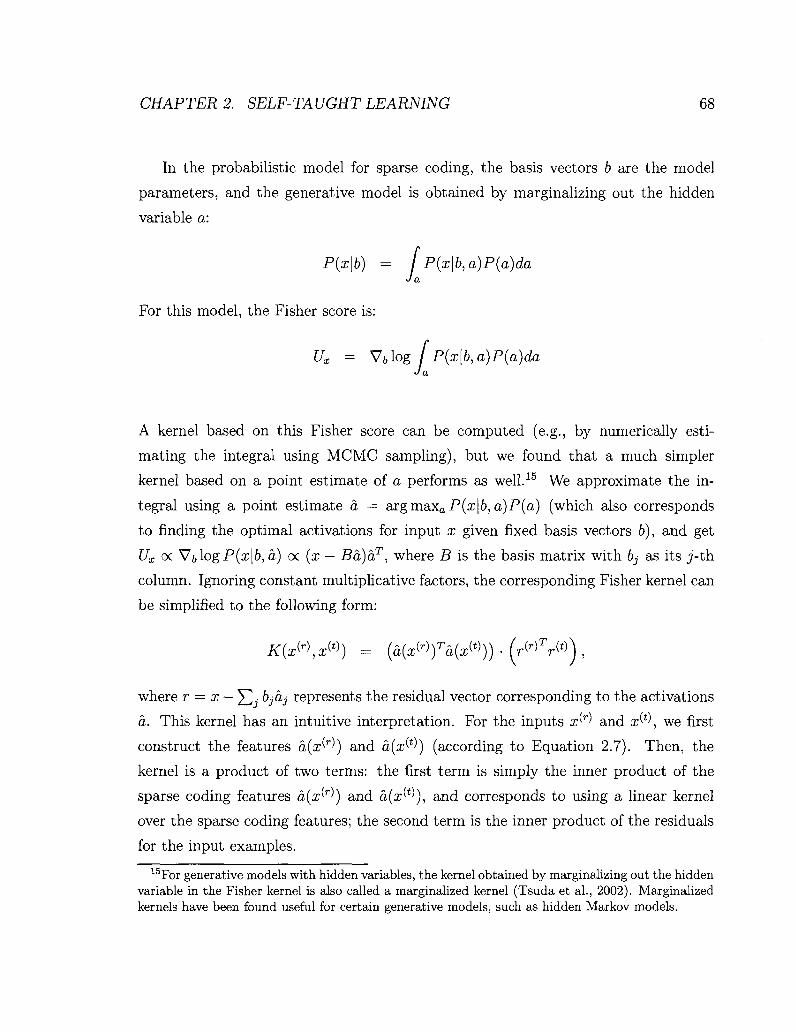
CHAPTER 2. SELF-TAUGHT LEARNING 68
In the probabilistic model for sparse coding, the basis vectors b are the model
parameters, and the generative model is obtained by marginalizing out the hidden
variable a:
P{x\b) = f P(x\b,a)P(a)da J a
For this model, the Fisher score is:
Ux = V6log / P(x\b,a)P(a)da J a
A kernel based on this Fisher score can be computed (e.g., by numerically esti
mating the integral using MCMC sampling), but we found that a much simpler
kernel based on a point estimate of a performs as well.15 We approximate the in
tegral using a point estimate a = argmaxaP(x|6, a)P(a) (which also corresponds
to finding the optimal activations for input x given fixed basis vectors £>), and get
Ux oc VblogP(a;|&, a) oc (x — Ba)aT, where B is the basis matrix with bj as its j-th.
column. Ignoring constant multiplicative factors, the corresponding Fisher kernel can
be simplified to the following form:
K(x<-r\x®) = (a(xW)Ta(xW))-(rWTrW),
where r = x — ]P bjd,j represents the residual vector corresponding to the activations
a. This kernel has an intuitive interpretation. For the inputs x^ and x^\ we first
construct the features a{x^) and a(x^) (according to Equation 2.7). Then, the
kernel is a product of two terms: the first term is simply the inner product of the
sparse coding features a(x^) and a(x^) , and corresponds to using a linear kernel
over the sparse coding features; the second term is the inner product of the residuals
for the input examples.
15For generative models with hidden variables, the kernel obtained by marginalizing out the hidden variable in the Fisher kernel is also called a marginalized kernel (Tsuda et al., 2002). Marginalized kernels have been found useful for certain generative models, such as hidden Markov models.
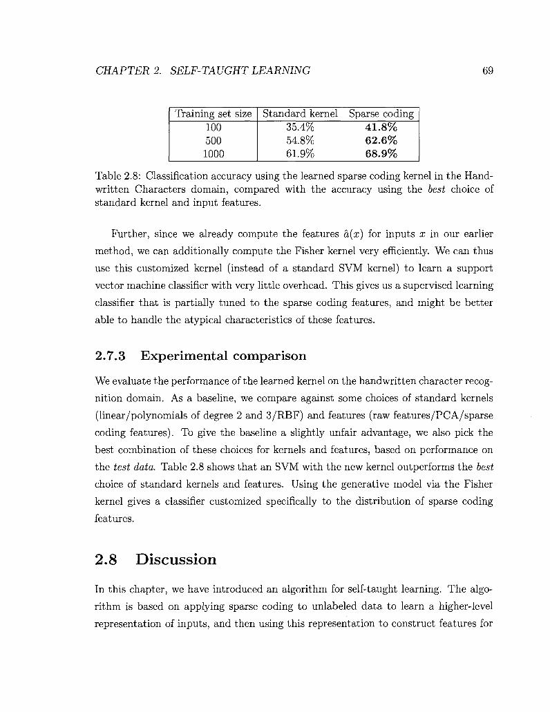
CHAPTER 2. SELF-TAUGHT LEARNING 69
Training set size 100 500 1000
Standard kernel Sparse coding 35.4% 41.8% 54.8% 62.6% 61.9% 68.9%
Table 2.8: Classification accuracy using the learned sparse coding kernel in the Handwritten Characters domain, compared with the accuracy using the best choice of standard kernel and input features.
Further, since we already compute the features a(x) for inputs x in our earlier
method, we can additionally compute the Fisher kernel very efficiently. We can thus
use this customized kernel (instead of a standard SVM kernel) to learn a support
vector machine classifier with very little overhead. This gives us a supervised learning
classifier that is partially tuned to the sparse coding features, and might be better
able to handle the atypical characteristics of these features.
2.7.3 Experimental comparison
We evaluate the performance of the learned kernel on the handwritten character recog
nition domain. As a baseline, we compare against some choices of standard kernels
(linear/polynomials of degree 2 and 3/RBF) and features (raw features/PCA/sparse
coding features). To give the baseline a slightly unfair advantage, we also pick the
best combination of these choices for kernels and features, based on performance on
the test data. Table 2.8 shows that an SVM with the new kernel outperforms the best
choice of standard kernels and features. Using the generative model via the Fisher
kernel gives a classifier customized specifically to the distribution of sparse coding
features.
2.8 Discussion
In this chapter, we have introduced an algorithm for self-taught learning. The algo
rithm is based on applying sparse coding to unlabeled data to learn a higher-level
representation of inputs, and then using this representation to construct features for

CHAPTER 2. SELF-TAUGHT LEARNING 70
a supervised learning classifier. We conclude the chapter with a discussion of some
unexplored connections and open questions for future work.
2.8.1 Biological comparisons
A longstanding hypothesis in computational neuroscience states that human percep
tual processing is tuned to the statistics of its natural surroundings. (Atick, 1992) For
example, it states that visual processing occurs the way it does because of the visual
nature of the world we live in; or, audio processing occurs the way it does because
of the audio surroundings we live in, and so on. This suggests that there might be
a general organizing principle, or a computational algorithm, that when applied to
percepts (images, audio, etc.) in the natural surroundings, can lead to human-like
perceptual processing. In fact, some neuroscientists believe that a lot of human intel
ligence can be attributed to a single algorithm (Mountcastle, 1978), a hypothesis that
has recently become popular with a broader public audience. (Hawkins & Blakeslee,
2004) As partial validation of this hypothesis, experiments have demonstrated that
the same piece of brain tissue can learn to process very different input modalities,
such as sight and sound, just by being exposed to inputs of those modalities (Sharma
et al., 2000). This further suggests that we may not need a different organizing prin
ciple each for vision, audio, touch, etc., but that a single organizing principle, or a
single learning algorithm, could be used to replicate intelligent, human-like perceptual
processing.
Against this background, the sparse coding model was originally developed as a
model for low-level mammalian perception, and it was demonstrated that sparse cod
ing (as well as some other algorithms, such as independent components analysis (van
Hateren & van der Schaaf, 1998)) applied to unlabeled input data (images, audio,
etc.) can learn basis vectors that resemble filters found in perceptual processing in
the mammalian brain (Hubel & Wiesel, 1962; Olshausen & Field, 1996a; Olshausen
& Field, 1997). For example, when sparse coding was applied to small image patches
extracted from images of natural scenes, the basis vectors converged to various kinds
of Gabor filters (edges), and closely matched the filters observed in low-level visual

CHAPTER 2. SELF-TAUGHT LEARNING 71
processing in the brain (in the visual cortex layer called "VI") (Olshausen & Field,
1997). When sparse coding was applied to audio inputs, the basis vectors converged
to audio patterns called gammatones, almost identical to those observed in low-level
audio processing in the brain (Smith & Lewicki, 2005). Sparse coding has also been
shown to exhibit other kinds of nonlinear phenomena, such as end-stopping (Sceniak
et al., 2001) and center-surround suppression (Cavanaugh et al., 2002; Series et al.,
2003), observed in the brain (Lee et al., 2007a).
In our view, the observed match between the results of sparse coding algorithms
and measured biological data is a significant bonus. While it is difficult to motivate
a machine learning algorithm purely based on match with biological data, a compar
ison with biological data may help direct future research via the following question:
given that sparse coding mimics characteristics of low-level visual/audio processing
in the brain, and that it also performs well on self-taught learning applications, what
new modifications or extensions are needed to also mimic higher-level visual/audio
processing, and thus hopefully obtain even better self-taught learning performance?
As a specific example, a different unsupervised learning algorithm, called the sparse
deep belief network (Lee et al., 2007b), was recently developed to explain observed
higher-level filters in the visual cortex layer called V2 (Ito & Komatsu, 2004; Boyn-
ton & Hegde, 2004; Levitt et al., 1994)—while the model was primarily validated
by showing that it matches measured biological data, the model also performs well
on machine learning tasks, such as image classification. With more detailed compu
tational studies of the brain being produced regularly, we believe that such fruitful
synergies between analysis of artificial (machine learning) and biological systems will
only increase in the future.
2.8.2 Theoretical guarantees
We posed the self-taught learning problem mainly to reduce the restrictions on the
types of data that we are allowed to learn from. As Table 2.1 shows, the unlabeled
and labeled data in our experiments were obtained in a natural way, with only a
minimal attempt to obtain both unlabeled and labeled data from the same "data

CHAPTER 2. SELF-TAUGHT LEARNING 72
type." Across these domains, self-taught learning empirically leads to significant
gains in classification accuracy. An important theoretical question is characterizing
how the "similarity" between the unlabeled and labeled data affects the self-taught
learning performance (similar to the analysis by Baxter, 1997, for transfer learning).
The self-taught learning formalism itself does not make restrictions on the types
of unlabeled data, but of course, we do need the unlabeled data to be "similar" to
the labeled data in some way—to take an extreme example, if the unlabeled data
were to consist of random (noise) images with random pixel intensities, while the
labeled data consists of handwritten characters, it is unlikely that we can benefit
from using the unlabeled data for learning. Similar theoretical statements have been
made about other formalisms such as semi-supervised learning (Ando & Zhang, 2005;
Ben-David et al., 2008; Zhu, 2005; Seeger, 2001) and transfer learning (Baxter, 1995;
Thrun, 1996; Ben-David & Schuller, 2003; Caruana, 1997), and we leave a similar
theoretical understanding of self-taught learning as an important open question for
future research.
We note that in our self-taught learning algorithm, the same probabilistic model
for sparse coding was used for both unlabeled and labeled data—the parameters b were
estimated using the unlabeled data, and then the latent activation variables a were
inferred for the labeled data using the learnt parameters b; these inferred activations
were finally used as features. While we did not make explicit assumptions about the
unlabeled and labeled data arising from the same distribution in self-taught learning
(as done in some semi-supervised learning algorithms, such as Nigam et al., 2000),
and did not use such distributional considerations explicitly in picking the unlabeled
and labeled data for our experiments, our sparse coding algorithm can be interpreted
as relying on the fact that both the labeled and unlabeled data can be fit well with a
common sparse coding probabilistic model, as shown in Figure 2.7. In our view, since
the model can use a large number of basis vectors, even larger than the original input
dimension,16 and multiplex different subsets of basis vectors for each input using the
latent activation variables a, this is a moderately weak restriction in practice. 16This is unlike PCA, for example, where the number of "basis vectors" (principal components)
must be less than the input dimension due to the orthogonality constraint between principal components.

CHAPTER 2. SELF-TAUGHT LEARNING 73
We believe that further exploration of this modeling assumption could lead to a
better theoretical understanding of precisely when our self-taught learning algorithm
might be expected to perform well, and answer a central question: Given labeled data
from a supervised classification problem, under what minimal theoretical assumptions
can we expect benefits from using unlabeled data?
2.8.3 Extensions to the sparse coding model
Our sparse coding formulation uses a nondifferentiable Li-penalty term. Especially
with a large number of basis vectors, the formulation encourages activations to be
sparse, and to only have nonzero activations for the few basis vectors that best match
the input vector. Sparse coding can have the property that a small modification in the
input x leads to a large change in the activations or features a(x), because a different
basis vector is now the best match for the modified input. In other words, the features
computed by our sparse coding algorithm can be "unstable," and this might affect
performance on some self-taught learning tasks. Recent work has shown that the
nondifferentiable Li-penalty can be replaced by a differentiable penalty based on the
KL divergence measure, to produce better self-taught learning performance (Bradley
& Bagnell, 2008). Other forms of regularization might also reduce the problems due
to instability—one such option could be an elastic net penalty (Zou et al., 2004),
that empirically leads to sparsity across groups of activations, instead of encouraging
sparsity for individual activations as in our sparse coding model.
In our work, we have not used the labeled data at all in the unsupervised feature
construction phase. When labeled data is extremely scarce (only a few available
examples), there is little other choice. But when moderate amounts of labeled data
are available, the sparse coding formulation can be modified to also encourage basis
vectors to model the labeled data well. One way to implement this modification would
be to explicitly encourage the learnt activations to be discriminative for the target

CHAPTER 2. SELF-TAUGHT LEARNING 74
classes, by adding an extra term to the sparse coding objective function:
minimize^ £ * \\x$ - £ , a f&J 2 + /?£< ||aW|U + 7 E i ? (&(*i(i))) (2.11)
s-t. 116,11 < 1, Vjel,...,s (2.12)
where q is some functon that measures the quality of the learnt features on the
labeled data (for example, by computing the log-likelihood achievable on labeled
data), and 7 is a parameter that specifies the relative importance given to the labeled
data. If q is a convex differentiate function of a and b separately, then our previous
alternating minimization algorithm can be adapted to this setting. A different way of
using labeled data to influence basis vectors would be to train initial basis vectors on
unlabeled data, and then fine tune the basis vectors on labeled data as well (Bradley
& Bagnell, 2008).
Our sparse coding algorithm is able to learn low-level features of the inputs. This
includes edge-like features for images, simple sound patterns for audio, and text topics
for text documents. For high-performance self-taught learning, we would want to
learn more complex features also. For example, for images, we might hope to learn
features that represent parts of objects ("wheel", "face", etc.), or whole objects ("car",
"apple", etc.). One way to achieve this would be to use a hierarchical model, that
computes not just features of the input, but also features of those features, features
of the features-of-features, and so on. This corresponds to learning a multilayer
representation, where each layer computes more complex features as output, given
the previous layer's features as input. Sparse coding has indeed been applied in two
layers (Hoyer & Hyvrinen, 2002), and it learns interesting, slightly higher-level filters
(such as larger contours instead of edges), though such a two-layer extension did not
lead to large gains on self-taught learning in our experiments. There is a lot of recent
work in learning such multilayer representations from unlabeled data using neural
network models (Hinton & Salakhutdinov, 2006; Lee et al., 2009a), and we expect
those models to be widely applicable to self-taught learning problems.
Chapter 3
Self-taught Learning for Audio
Classification
In this chapter, we focus on the application of our self-taught learning algorithms to
audio classification. To motivate later discussion, consider a speaker identification
task in which we'd like to distinguish between Adam and Bob from their speech with
only a few seconds of labeled speech samples from Adam and Bob as training data.
Given only a few seconds of speech samples as labeled training data, this is a difficult
task to solve well using only supervised learning techniques. For such a task, semi-
supervised learning algorithms can make use of additional unlabeled data that has the
same class labels as the classification task (Nigam et al., 2000). Thus, to apply most
semi-supervised learning methods (such as the method of Nigam et al. (Nigam et al.,
2006)) to distinguish between Adam and Bob, we must obtain additional unlabeled
data from Adam and Bob specifically. This sort of unlabeled data is hard to obtain;
indeed, short of eavesdropping on conversations between Adam and Bob, it is hard
to envisage a data collection method that results in unlabeled speech samples from
Adam and Bob—and no one else—that does not also automatically result in our
having the class labels as well. Transfer learning typically attempts to use additional
labeled data to construct supervised classification problems that are related to the
task of interest (Caruana, 1997; Thrun, 1996; Ando & Zhang, 2005). Thus, for
speaker identification, transfer learning may require labeled data from other speech
75

CHAPTER 3. SELF-TAUGHT LEARNING FOR AUDIO CLASSIFICATION 76
classification tasks. Since these additional classification tasks are supervised and thus
require labeled examples, data for even transfer learning is often difficult to obtain.
In contrast, the self-taught learning framework introduced in the previous chapter
attempts to use easily obtainable unlabeled data to improve classification perfor
mance. For the task of distinguishing between Adam and Bob, this means we may
use unlabeled data from speakers other than Adam and Bob (or perhaps even use
non-speech audio samples). Given the ease with which such data can be obtained—
one can envisage recording audio from radio broadcasts or downloading audio clips
randomly off the internet—we believe that self-taught learning holds the promise of
much easier applicability than most semi-supervised learning and transfer learning
algorithms.
In principle, the sparse coding algorithm discussed in the previous chapter can
be directly applied to audio classification. For illustration, consider a 500ms speech
signal sampled at 16kHz. The raw acoustic signal is a vector x € R8000 containing
the time-domain amplitude values that constitute the signal. This unwieldy repre
sentation can be extremely difficult to reason over. Instead, our self-taught learning
algorithm discovers statistical correlations from unrelated unlabeled data, and thus
learns a "dictionary" of 200 basis vectors (say) that, when superposed only a few at a
time, suffice to adequately describe most input audio signals. Given a 500ms speech
signal, the algorithm might be able to represent the signal using just 10 (say) of these
learnt basis functions. Informally, the algorithm is able to describe the 8000 numbers
succinctly using only 10 numbers corresponding to the activated basis vectors, leading
to a succinct representation that is significantly easier to reason with. (See Figure
la.)
In the example of speech, we can informally think of the audio speech signal as
being generated by a small number of distinct acoustic events, such as vibrations
of the vocal cords. These underlying acoustic events might provide a concise and
relatively noiseless representation of the signal; they also provide a slightly higher-
level representation that might be easier to reason with than the raw acoustic signal.
This is analogous to the image representation example considered in the previous
chapter—visual signals (images) can be encoded efficiently as a combination of only
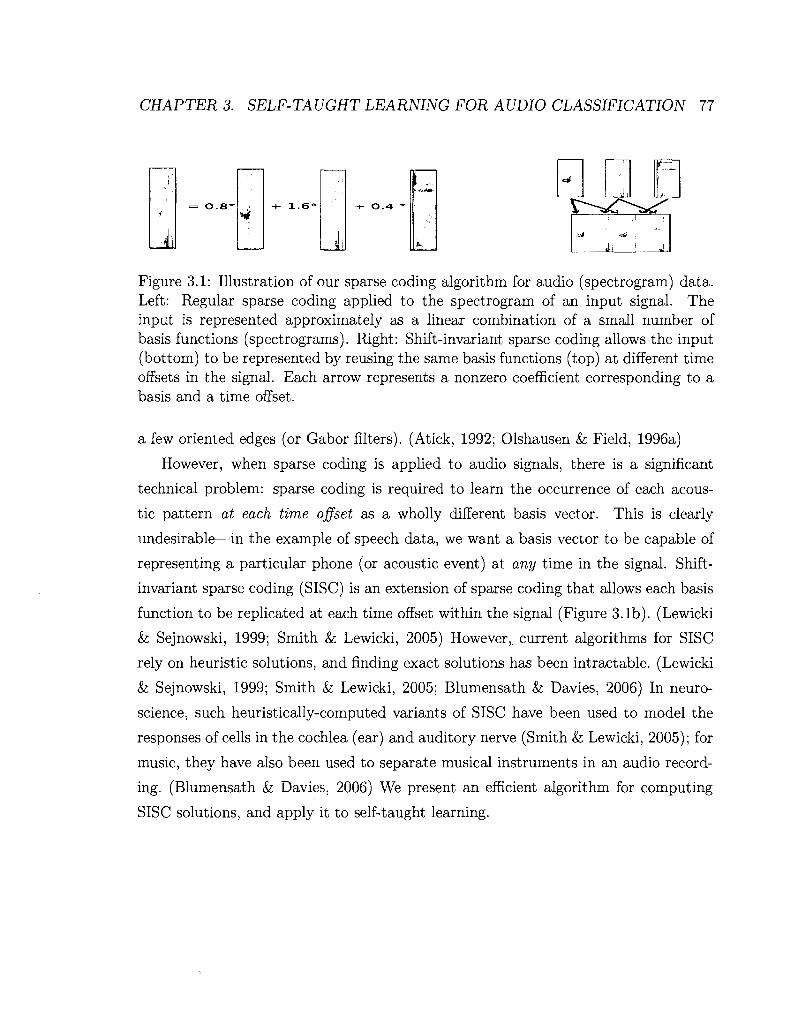
CHAPTER 3. SELF-TAUGHT LEARNING FOR AUDIO CLASSIFICATION 77
Figure 3.1: Illustration of our sparse coding algorithm for audio (spectrogram) data. Left: Regular sparse coding applied to the spectrogram of an input signal. The input is represented approximately as a linear combination of a small number of basis functions (spectrograms). Right: Shift-invariant sparse coding allows the input (bottom) to be represented by reusing the same basis functions (top) at different time offsets in the signal. Each arrow represents a nonzero coefficient corresponding to a basis and a time offset.
a few oriented edges (or Gabor filters). (Atick, 1992; Olshausen k Field, 1996a)
However, when sparse coding is applied to audio signals, there is a significant
technical problem: sparse coding is required to learn the occurrence of each acous
tic pattern at each time offset as a wholly different basis vector. This is clearly
undesirable—in the example of speech data, we want a basis vector to be capable of
representing a particular phone (or acoustic event) at any time in the signal. Shift-
invariant sparse coding (SISC) is an extension of sparse coding that allows each basis
function to be replicated at each time offset within the signal (Figure 3.1b). (Lewicki
& Sejnowski, 1999; Smith & Lewicki, 2005) However, current algorithms for SISC
rely on heuristic solutions, and finding exact solutions has been intractable. (Lewicki
& Sejnowski, 1999; Smith & Lewicki, 2005; Blumensath & Davies, 2006) In neuro-
science, such heuristically-computed variants of SISC have been used to model the
responses of cells in the cochlea (ear) and auditory nerve (Smith & Lewicki, 2005); for
music, they have also been used to separate musical instruments in an audio record
ing. (Blumensath & Davies, 2006) We present an efficient algorithm for computing
SISC solutions, and apply it to self-taught learning.

CHAPTER 3. SELF-TAUGHT LEARNING FOR AUDIO CLASSIFICATION 78
3.1 Shift-invariant Sparse Coding
Recall the sparse coding model used in the previous chapter: given unlabeled exam
ples {xu, xu , • • •, xu } where Xu G Rn, the sparse coding model finds basis vectors
{&!,b2,. •., bs} where bj G Rn, and activations a/-' by solving the following optimiza
tion problem:
minimize^ £ \ \\x® - E,<4%-||2 + /?£» ll«Wlli (3-1)
s.t. H&JII < 1, V? G l,...,s (3.2)
In shift-invariant sparse coding (SISC), each basis basis vector is allowed to appear
at all possible shifts within the signal. (Lewicki & Sejnowski, 1999; Smith & Lewicki,
2005) Given inputs x^ G Rn, SISC finds basis vectors {bu b2,..., bs} where bj G Rq—
the basis vectors bj can be of lower dimension than the input signal itself (q < n)
to allow a basis vector to represent only part of the input vector. To represent the
activation of basis vector bj for input Xu at each time offset, we now need a vector
of activations a? G Mn_9+:L, such that the t-th element in this vector a? represents
the activation of basis vector bj in the input x{, at time offset t. Note that sparse
coding as discussed in the previous chapter corresponds to the special case where
n = q, and the activation a- G R is just a single real number. In our earlier
example, if each input xi° G R8000 is a 500ms-long speech signal, we might choose
to avoid redundancy by using 100ms-long basis vectors, in which case bj G R1600.
Further, the activation corresponding to the input Xu and basis bj is now a vector
at1' G R8000_1600+1, representing the activation for each possible temporal starting
offset for the basis a^\ We will use the notation a^T to represent the coefficient
corresponding to the input Xu, basis a ^ and temporal offset t.
For shift-invariant sparse coding, we can use the convolution operator * to con
cisely represent our approximation of the input Xu as a superposition of basis func
tions: Xu ~ E7 fy * aj -1
JIf h = f * g is the 1-D discrete convolution of two vectors f £ MP and g £ RQ, then ht = S™=^^(i,*-9+i) fT9t~r+i- The dimension of the vector h is given by dim(ft) = dim(/) +dim(sO - 1 -For ease of exposition, we present our SISC model and algorithms only for audio or other sequential

CHAPTER 3. SELF-TAUGHT LEARNING FOR AUDIO CLASSIFICATION 79
To use ideas recently developed for solving the sparse coding model, we pose the
SISC problem as the natural extension to the sparse coding optimization problem (3.1-
3.2):
minimize^ £ . ||a#> - ^ h * aff + / ? £ \ . \\af\\x (3.3)
s.t. M&j|| < 1, V j e l , . . . , s (3.4)
Note that by explicitly representing the basis vector at each time offset as a separate
basis vector variable, and expanding out the convolution in terms of these new vari
ables, we can, in principle, formulate the above optimization problem as a very large
sparse coding problem similar to problem (3.1-3.2)—with the additional constraint
that the basis vector variables corresponding to different shifts contain tied param
eters. However, such a reformulation would lead to an optimization problem with
many more optimization variables—to model 6400 different time offsets (as in the
above example), we need 6400 times as many basis vectors. This ignores the special
structure in the problem (3.3-3.4), and is computationally infeasible to solve for even
moderate problem sizes. Previous solutions to similar SISC optimization problems
have thus been based on heuristics. (Lewicki & Sejnowski, 1999; Smith & Lewicki,
2005; Blumensath & Davies, 2006) Instead, we use techniques from our sparse coding
algorithms to efficiently solve the SISC problem.
3.2 Efficient SISC Algorithm
We solve the optimization problem (3.3-3.4) by alternately solving two large convex
optimization problems: minimizing over the activations a? given a fixed basis set,
and minimizing over the basis vectors bj given the activations. We now describe
efficient algorithms for each of these problems.
(1-D) signals. However, the model and algorithm can also be straightforwardly extended to other input signals with spatial and/or temporal extent (such as images or videos), by using higher-order convolution operators.

CHAPTER 3. SELF-TAUGHT LEARNING FOR AUDIO CLASSIFICATION 80
3.2.1 Solving for activations
Given a fixed set of basis vectors b, the optimization problem (3.3-3.4) over activations
a decomposes over i = 1 , . . . , k into a set of k independent optimization problems. In
other words, the activations {a^ , j = 1 , . . . , s} corresponding to an input x^ can
be found independently of the activations corresponding to other inputs. Thus, we
will focus on the problem of finding the activations a corresponding to a single input
x® G W1:
minimizea \\x® - £ \ bj * a j 2 + PY,j IKIk (3-5)
Here, dj G ]Rn_9+1 represents the activations associated with basis bj. Optimiz
ing (3.5) with respect to a is difficult because there are many optimization variables,
and they are highly coupled. (For instance, recall that the activation Ojl for a basis
vector at one time instant and the activation CL^I+I f° r the same basis vector at the
next instant are two distinct variables. A basis vector typically correlates quite highly
with the same basis vector shifted by one timestep, and this makes it hard to deter
mine which of the two activations better "explains" the input signal x^.) Previous
work (Smith & Lewicki, 2005; Blumensath & Davies, 2006) computed activations
using gradient descent on the objective function (3.5). Gradient descent does not
typically work well with problems whose variables are tightly coupled. Most existing
implementations, therefore, use a heuristic to select a subset of the activations to op
timize, and set the other activations to zero. As we demonstrate in the experiments
section, the tight coupling between activations makes it difficult to heuristically se
lect a small subset of variables to optimize, and as a result, such heuristic techniques
typically lead to suboptimal solutions.
Our approach will efficiently find the exact optimum with respect to all the activa
tions by taking advantage of the "feature-sign" trick described briefly in the previous
chapter: the Li-regularized least squares problem (3.5) reduces to an unconstrained
quadratic optimization problem over just the nonzero activations, if we are able to
correctly guess the signs (positive, zero or negative) of the optimal values of the ac
tivations. Such a quadratic optimization problem can then be easily solved in closed

CHAPTER 3. SELF-TAUGHT LEARNING FOR AUDIO CLASSIFICATION 81
form using standard numerical methods. This feature-sign trick has been formalized
in the feature-sign search algorithm, which greedily searches the space of nonzero ac
tivations and their signs, and provably converges to the optimal solution. (Lee et al.,
2007a)
The feature-sign search algorithm can be modified to efficiently compute activa
tions for short signals (i.e., when x^ is low-dimensional), as shown in Algorithm 2.2
For example, if fewer than 1000 activations are nonzero over the course of the opti
mization for problem (3.5) (and at its optimal solution), then each of the quadratic
optimization problems solved in the inner loop of feature-sign search will also involve
at most 1000 variables, so that they can be solved efficiently. However, we are often
interested in solving for the activations corresponding to fairly long signals (such as if
x^ is a 1 minute long speech signal). Empirically, the number of nonzero activations
in the optimal solution grows roughly linearly with the length of the signal (i.e., the
dimensionality of x^). Since solving each least squares problem takes about 0(Z3)
time for Z nonzero activations, the standard feature-sign search algorithm becomes
expensive for long signals.
To address this problem, we use an iterative sliding window approach as shown
in Algorithm 3 to solve a series of smaller problems using the feature-sign search
algorithm. These smaller problems are generated by attempting to solve for only 2q
activations at one time, while keeping the other activations fixed, and iterating till
convergence. In solving for these activations using feature-sign search, we can also
set the signs of the activations to enable the feature-sign trick: activations which
were nonzero keep their sign, all other activations that are in the current window
W are assigned a sign opposite to the sign of their partial derivative (so that if
an activation has a negative partial derivative of the quadratic term, it is assigned
a positive sign for feature-sign search), and any other activations are set to zero.
Since the objective function in problem (3.5) is convex, this method is guaranteed to
2Other details: Feature-sign search activates activations one at a time, because this is necessary for guaranteeing a descent direction. In our implementation, for each iteration, we simultaneously activate the T = 300 zero activations with the largest partial derivatives. This is not guaranteed to give a descent direction, but in the (extremely rare) case where it does not, we simply revert to choosing a single activation for that particular iteration. This preserves the theoretical convergence guarantee of feature-sign search.

CHAPTER 3. SELF-TAUGHT LEARNING FOR AUDIO CLASSIFICATION 82
Algorithm 2 FS-EXACT
input Input x® € W1, basis vectors b\, b2, • • •, bs G R9, step size parameter T. output Optimal activations a,j G Mn_9+1 for problem (3.5). algorithm
Initialize a,j := 0, or to value from previous iteration. while true do
S:={a®\a®*0} S := S U {up to T activations not in S with the largest (magnitude) partial derivatives of the quadratic term \\x® — ^ - bj * a | | 2 } . Solve (3.5) exactly for the activations in S using FS-EXACT, assuming all activations not in S are set to zero. Break if the partial derivatives of the quadratic term w.r.t. all the activations are smaller than /?.
end while return the optimal activations a (i)
Algorithm 3 FS-WINDOW input Input x^ e Rn, basis vectors b\, b2, • • •, bs e M9. (Assume for simplicity that
n - q + 1 is divisible by q.) Algorithm parameters: Npasses, Nwindows. output Estimated activations a^ G Rn _ 9 + 1 for problem (3.5). algorithm
Initialize a? arbitrarily, or to value from previous iteration. numwindows := (n — 2q + l)/q. for pass = 1 to Npasses do
for w = 1 to Nwindows do W := {af\g(w - 1) + 1 < i < q{w + 1)} Solve problem (3.5) exactly for the activations in W using feature-sign search, keeping all activations not in W fixed.
end for end for return the estimated activations aS; .

CHAPTER 3. SELF-TAUGHT LEARNING FOR AUDIO CLASSIFICATION 83
converge to the optimal solution. We will refer to plain feature-sign search (without
the sliding window) as FS-EXACT and feature-sign search with sliding window as
FS-WINDOW.
Importantly, even though in the worst case the sliding window approach would
only be expected to converge linearly, and require a large number of passes through
the signal to estimate the optimal activations, in all of our experiments (images,
speech, and music), the value obtained for the optimization objective after only two
passes through the signal was only a tiny fraction of a percent worse than the optimal
value. This is because the activation values that correspond to very different time
offsets (for example, if the offsets are further than q time offsets apart), are generally
not very tightly coupled, and can thus be optimized sequentially rather than jointly.
With a small, fixed number of passes through the signal, the observed performance for
optimizing over a single window still depends on the number of nonzero activations
Zw in that window as O(Z^), but does not grow as 0(Z3) if Z is the number of
nonzero activations in the full signal. Empirically, FS-WINDOW is much faster than
FS-EXACT with very little loss in accuracy.
3.2.2 Solving for basis vectors
Lee et al. (2006) presented an efficient method to optimize the sparse coding opti
mization problem (3.1-3.2) with respect to the basis vectors bj for fixed activations:
minimize6 £V \\x£ - YJJ ajbj\\2 (3-6)
s.t. H&jll < 1, V? E l,...,s (3.7)
Their algorithm used the insight that the quadratic objective function can be writ
ten as a sum of s quadratic terms, each penalizing the reconstruction error for one
element of xi, , and depending only on a subset of all the basis vector elements
{bi,u &2,t> j • • •, bsj} for some fixed element number t (1 < t < q), where bjyt denotes
the t-th element of basis vector bj. This therefore decomposes the optimization prob
lem (3.6-3.7) into many smaller, nearly-independent problems (that are coupled only
through the normalization constraint in Equation 3.7). By transforming the problem

CHAPTER 3. SELF-TAUGHT LEARNING FOR AUDIO CLASSIFICATION 84
into the equivalent, dual optimization problem, it could then be solved very efficiently.
Unfortunately, the same is not true for SISC. Solving the SISC optimization prob
lem (3.3-3.4) for the basis vectors b keeping the activations a fixed reduces to a con
strained quadratic optimization problem:
minimize;, Y^i \\xu - Ylj bj * aj II2 (3-8)
s.t. \\bjW < 1, Vjel,...,s (3.9)
In this problem, because each basis vector can appear in any possible shift (temporal
offset), each component of the basis vector contributes to reconstructing many dif
ferent elements of an input x„ , and thus contributes to many different terms in the
objective function. Therefore, unlike sparse coding, the different components of the
basis vectors are more tightly coupled in the objective. However, as we now demon
strate, this problem is much easier to solve when transformed into the frequency
domain.
For a basis vector bj = (bjti, b^, • • •, bj>q), let the discrete Fourier transform (DFT)
be denoted by bj = (bjti, bj$, • • •, bj<q), where each element bjtT is a complex number,
representing the frequency component r.3 We will use the following two facts from
signal processing theory to simplify optimization problem (3.8-3.9): (i) Parseval's
theorem (Oppenheim et al., 1996) implies that the DFT bj of a vector bj scales the
L2 norm by a constant factor; in other words, ||6j|| = -K"||bjJ|, where K is a known
constant.4 Since our objective and constraints both consist of L2 terms, we can apply
the DFT to them to obtain an equivalent optimization problem over bj instead of bj.
(ii) The Fourier transform of a convolution is the elementwise product of the Fourier
transforms. Using (i) and (ii), and denoting the elementwise product of vectors / and
3Following standard practice, we apply the DFT after padding the basis vector bj with zeros so as to make it the same length n as the inputs x. In this case, the DFT is also of length n. Due to space constraints, we refer the reader to standard texts such as Oppenheim et al. (Oppenheim et al., 1996) for further details on Fourier transforms.
4Note that the DFT may contain complex numbers. We use C to denote the set of complex numbers, and y* to denote the conjugate transpose of a complex vector y e C". The L^ norm of a complex vector y £ C n is defined as \\y\\ = y/y*y.

CHAPTER 3. SELF-TAUGHT LEARNING FOR AUDIO CLASSIFICATION 85
9 by / • g, the optimization problem becomes:
E ll "(i) V~> i. " ( J ) 112 i\\xu -2^jbj'aj \\
s.t. \\bj\\ < c = K, Vj G l,...,s
where the optimization is now over the vector of complex variables bj G Cn, and
Xu G Cn and d^ G Cn represent the complex-valued DFT for the input Xu and
(padded) activations a* respectively. Now, for this problem, the variables are no
longer tightly coupled, and the Lagrangian can be decomposed as a sum of quadratic
terms, each depending on a single frequency component r:
C{b,X) = ] P (\\xT - ArvT\\2 + v*AvT} - c J ^ A j ,
with dual variables A G Rs and
/ *S \ / kr \
(*) \ %U,T I
G Cfc, vT = I i G C s , A = diag(A) G E s x s ,
i T = | a!2! a?> ... | G C
V
kxs
)
The Lagrangian C(b, A) is a function of complex variables 6, but can be expressed as
a function of only real variables by representing the real and imaginary parts of b as
separate real-valued variables. Further, since \y\2 = |Re(y)|2 + |Im(y)|2 for a complex
number y, we can analytically compute bmm = argmin^£(6, A) by optimizing over
Re(fi) and Im(d) to obtain:5
= (A*TAT + A) A*TxT r (3.10)
5This can be proved by closely following the derivation for the Lagrangian with real-valued variables, as demonstrated by Lee et al. for the sparse coding algorithm (Lee et al., 2007a).
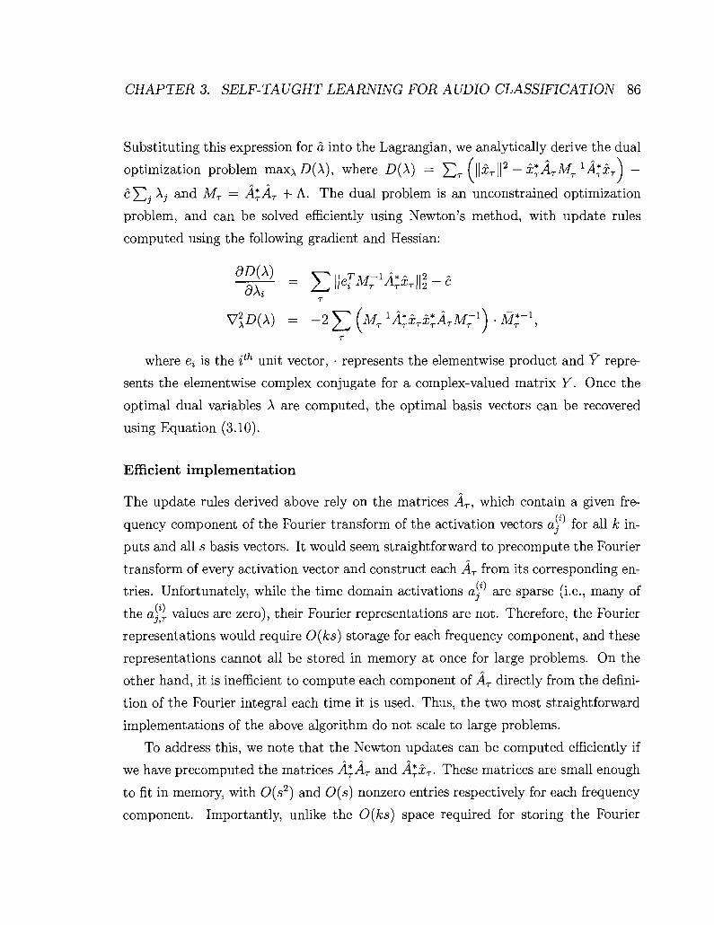
CHAPTER 3. SELF-TAUGHT LEARNING FOR AUDIO CLASSIFICATION 86
Substituting this expression for a into the Lagrangian, we analytically derive the dual
optimization problem maxA-D(A), where D(\) = Ylr (ll^H2 — X^ATM*1 A^Xr J —
c Y^j \ a n d Mr = A*TAT + A. The dual problem is an unconstrained optimization
problem, and can be solved efficiently using Newton's method, with update rules
computed using the following gradient and Hessian:
^ = YlhJ^KxT\\l-c T
V\D{\) = -2^(M- 1 i ;£ T x; i T M T - 1 ) -M*-\ T
where ej is the ith unit vector, • represents the elementwise product and Y repre
sents the elementwise complex conjugate for a complex-valued matrix Y. Once the
optimal dual variables A are computed, the optimal basis vectors can be recovered
using Equation (3.10).
Efficient implementation
The update rules derived above rely on the matrices AT, which contain a given fre
quency component of the Fourier transform of the activation vectors a?' for all k in
puts and all s basis vectors. It would seem straightforward to precompute the Fourier
transform of every activation vector and construct each AT from its corresponding en
tries. Unfortunately, while the time domain activations of' are sparse (i.e., many of
the a^l values are zero), their Fourier representations are not. Therefore, the Fourier
representations would require 0(ks) storage for each frequency component, and these
representations cannot all be stored in memory at once for large problems. On the
other hand, it is inefficient to compute each component of AT directly from the defini
tion of the Fourier integral each time it is used. Thus, the two most straightforward
implementations of the above algorithm do not scale to large problems.
To address this, we note that the Newton updates can be computed efficiently if
we have precomputed the matrices A*TAT and A*TxT. These matrices are small enough
to fit in memory, with 0(s2) and O(s) nonzero entries respectively for each frequency
component. Importantly, unlike the 0(ks) space required for storing the Fourier

CHAPTER 3. SELF-TAUGHT LEARNING FOR AUDIO CLASSIFICATION 87
transforms of all activation vectors, these figures do not depend on the number of input
signals k. Two further optimizations were used for our largest scale experiments: (i)
Because the discrete Fourier transform of a real signal is conjugate symmetric, A*AT
and A*TxT need to be explicitly computed and cached only for half of the frequencies
r. (ii) Since A*AT is Hermitian, it suffices to cache only the entries in the lower-
triangular part.
3.3 Constructing features using unlabeled data
We now describe an application of SISC to self-taught learning, where the goal is
to use unlabeled data to improve performance on a classification task. Here, the
unlabeled data may not share the classification task's labels.
In self-taught learning, we are given a labeled training set {(x\ \y\ ) , . . . , (x\m \ y\. }
together with k unlabeled examples {x^\ . . . , x^}. In the previous chapter, we pro
posed the following algorithm for self-taught learning: sparse coding is applied to the
unlabeled data x® to learn the basis vectors bj, by solving the optimization prob
lem (3.1-3.2). These learnt basis vectors are then used to construct features for each
input x\ to the classification task by computing:
a(xj ) = argmin||:£; — /_]^jaj\\2 + ^ llalli j
These features a(x\ ) can then be used as input to off-the-shelf classification algo
rithms such as an SVM or Gaussian discriminant analysis (GDA), and this often
produces better generalization performance than using the raw inputs xf them
selves. (Raina et al., 2006; Raina et a l , 2007)
However, the above approach is computationally infeasible and conceptually un
satisfactory when applied to representing "large" inputs with spatial and temporal
extent, such as images or audio. As a heuristic solution, in the previous chapter,
sparse coding was applied to small parts (or "patches") of the input images or audio
signals, and then the activations produced for these individual parts were aggregated

CHAPTER 3. SELF-TAUGHT LEARNING FOR AUDIO CLASSIFICATION 88
(e.g., by taking the sum of squares of all activations corresponding to a basis) to pro
duce a representation for the entire image or audio signal. Further, the learnt feature
representation a(x\ ) is not invariant to shifts of the input signal, and different basis
vectors might capture the same pattern occurring at different shifts.
To address these problems, we propose the following algorithm for self-taught
learning using SISC: We first apply SISC to the unlabeled data Xu to learn shift-
invariant basis vectors bj. The learnt basis vectors are then used to construct features
for the labeled inputs x\ by solving the SISC optimization problem:
a(i) = a r g m i n U x ^ - ^ 6 j * a J | | 2 + /? ||a||i. (3.11) i
Here, we will write a,jt € R to represent the activation found for basis bj at time t, and
a I = \fli\, a21, • • •, 6 ^ ] T G Rs to represent the vector of all activations (one activation
value per basis vector bi,...,bg) at time t. As in sparse coding, we expect the SISC
features a^1 to capture higher-level patterns than the raw input x\f . These features
are also robust to shifts and translations of the inputs in the following sense: if the
input signal is shifted by a certain amount in time, the features are also shifted by the
same amount, without any change in their relative values. Using these features aSl">
to represent the data, we will apply standard, off-the-shelf classification algorithms
(SVM and GDA) to learn a classifier.
We delve deeper into the application of the GDA learning algorithm to SISC
features. GDA posits that the conditional distribution of the features given the class
label is Gaussian. By assuming that the features a.l at time t are conditionally
independent of the features a t, at some other time t' given the label yf\ we get:
P{a{i)\y?)=y) = X[P(^\y?) = y) (3.12) t
where P(a)lJ \y) is modeled as a multivariate Gaussian (whose parameters \iy G Rs, T,y £
R s x s depend on y): a.*l ~ J\f([iy(i), Hy^). The GDA parameters fiy and Ey, and the
label priors P(y), are learnt using maximum likelihood on the labeled training data,
and test examples x are then classified by picking the label y* = argmax^ P(y\a) ==

CHAPTER 3. SELF-TAUGHT LEARNING FOR AUDIO CLASSIFICATION 89
argmaxy P(a\y)P(y), where a are the SISC features for input x.
In our experiments, we found that the SISC features a^ are poorly modeled by
a multivariate Gaussian generative distribution as used in GDA—a large number of
features are zero and the nonzero feature distributions have long tails.6 The nonzero
features empirically appear to follow an exponential distribution. We thus propose an
additional classification algorithm for SISC features, based on the following two-step
generative model for the features a^: each feature's sign (positive, negative, or zero)
is determined, and if its sign is nonzero, its value is then determined according to
an exponential distribution. Concretely, given y, for each a^t, we imagine that first
a random variable Z*j. £ {+,0,—} is drawn from a 3-way multinomial distribution
governed by parameter 0^ GR3. Z^J will determine the sign of a^t. Then, if Z^J. =
"+", we generate d^t ~ Exponential(p|'+); if Z^j. = "0", we set a^j. = 0; and lastly if
ZjJ = "—", we generate — a^j. ~ Exponential^ ' -) . Here, (jxj, p^'+ and p^'~ are the
parameters of the model, and define a naive Bayes like generative model: P(a^\y) =
Y\t Y[j P{Q>j,t\y)- The maximum likelihood parameters for the generative model are
straightforward to obtain,7 and are then used to compute label probabilities P{y\a^)
using Bayes' rule. We call this model "Exp," and present results on all domains using
the SVM, GDA and Exp classification algorithms.
Self-taught Learning Details
We apply the above self-taught learning algorithm to audio classification tasks. Rather
than use entire speech sentences or songs for the input vectors x£ , we found it was
much more efficient to divide the signals into medium-sized excerpts of 500 ms, which
would be treated as independent. This way, given a fixed set of basis vectors, the
optimal activations could be computed efficiently for each excerpt. To reduce edge
effects, each segment was multiplied by a window function which decays smoothly to
6 Some of the baseline features presented in the Experiments section, such as MFCCs, are most often modeled with a Gaussian distribution.
7Each multinomial parameter is estimated as a (smoothed) fraction of the occurrences of the feature with negative/zero/positive sign. Each exponential scale parameter p is estimated as the absolute value of the (smoothed) average of the feature values with the corresponding negative/positive sign.

CHAPTER 3. SELF-TAUGHT LEARNING FOR AUDIO CLASSIFICATION 90
zero near the start and end points. For faster convergence, we randomly divided the
training data into 2 batches and alternately optimized with respect to each batch.
3.4 Algori thm Efficiency
We begin by evaluating the running-time of our algorithm, described in Section 3.2.1,
for solving for the activations given a fixed basis set. To the best of our knowledge,
all previous algorithms for large-scale shift-invariant sparse coding have learned the
activations using a heuristic to preselect a subset of activations to optimize for (setting
all other activations to zero). Smith & Lewicki (2005) used matching pursuit and filter
threshold algorithms to select a subset of the activations to optimize for; we will refer
to the matching pursuit heuristic as the SL heuristic. Blumensath & Davies (2006)
used a heuristic which iteratively chooses the activation with the largest magnitude
gradient, and removes its "neighbors" (activations corresponding to the same basis
with a slightly different shift) from consideration; we will call this the BD heuristic.
In our implementation of each of these heuristics, we used gradient descent with line
search to optimize for the selected activations.8 We will compare these heuristics with
our exact activation learning algorithm (FS-EXACT) and gradient descent applied
to all the activations without any preselection (GD-FULL).9
Figure 3.2(a) shows the convergence rates of these four algorithms when applied to
learning SISC activations for a one-second (time-domain) speech signal using 32 basis
vectors.10 The suboptimality of an algorithm achieving objective /aig for problem (3.5)
with optimal objective /* is defined as (Aig —/*) / /*• FS-EXACT clearly outperforms
8Our gradient descent algorithm for solving min s / ( s ) + /3||s||i (for a differentiate function / ) transforms it to the equivalent problem min.s+,5- / ( s + — s~) + /3lT(s+ + s~) with the constraints s+,s~ > 0. The algorithm then performs a line search with exponential backoff along the negative gradient of the new objective function, handling the constraints by projecting all points considered during the line search into the feasible space. The algorithm exits when the cumulative decrease in the objective function over 3 iterations is less than a fixed threshold. This gradient descent algorithm was faster than a gradient descent algorithm using a constant step size.
9We do not present running time results for the faster sliding window algorithm FS-WINDOW as the exact algorithm FS-EXACT is usable at the scales for which results have been reported for previous algorithms.
10Each speech basis was 188ms long. Similar results were obtained when a straightforward extension of our method was applied to the case of 2-D convolution for images.

CHAPTER 3. SELF-TAUGHT LEARNING FOR AUDIO CLASSIFICATION 91
the other algorithms. For example, after 8 seconds, FS-EXACT is 10-2-suboptimal,
but it takes the best other algorithm 40 seconds to reach this level of suboptimality.
Further, even when given sufficient time to run the heuristics to convergence, both
the heuristic methods converge to suboptimal solutions, which are significantly poorer
than the solutions found by FS-EXACT. This is true even when the heuristic is
allowed to choose a substantial fraction of the activations to be nonzero (which slows
the heuristic methods further).
We next assess the effectiveness of using the dual problem formulation (in the
Fourier domain) for learning the basis vectors. We compare the overall running
time of basis learning using four possible algorithms, comprising combinations of
two methods for solving for the activations—FS-EXACT and GD-FULL—and two
methods for updating the basis vectors—Newton's method with the dual formulation
(DUAL) and stochastic gradient descent (GD-BASIS) on the original problem (3.3-
3.4). Figure 3.2(b) shows the convergence results for all four algorithms on the SISC
image task (similar results are achieved for the speech task). FS-EXACT + DUAL
outperforms the other algorithms. For example, it achieves an objective value of
1.74 x 10⁵ within 10 minutes, but the best other algorithm takes over 2 hours.
The overall time for solving the SISC optimization problem is dominated by the
time for learning activations. We also note that the two basis vector update methods
(DUAL and GD-BASIS) individually take comparable amounts of time per iteration,
even though the DUAL method computes the optimal basis vectors for the fixed
activations at each iteration, whereas GD-BASIS just updates the basis vectors using
a small gradient step at each iteration. This contributes to faster overall convergence
of basis learning using DUAL.
3.5 Self-taught Learning Results
We apply our SISC based self-taught learning algorithm to two audio classification
tasks: (i) Speaker identification on the TIMIT speech corpus (Garofolo et al., 1993)
given a small amount of labeled data (one sentence per speaker), and a large amount
of unlabeled data comprising speech from different speakers from different dialect

CHAPTER 3. SELF-TAUGHT LEARNING FOR AUDIO CLASSIFICATION 92
I U
10°
f 1°~2
£ Q. O -4 •§ 10 CO
10'6
i n 8
1 1 — • 1
—FS-EXACT --GD-FULL
BD heuristic —SC heuristic
\
\
10 20 30 Time (seconds)
(a)
40
,x10
60 SO Time (minutes)
(b)
120 140
Figure 3.2: (a) Convergence of activation learning for speech data. The plot shows the "suboptimality" achieved by the algorithms vs. the time taken (seconds). Similar results are obtained for 2-D image data, (b) Convergence of the SISC optimization problem for image data. The plot shows the objective value attained by different combinations of activation learning and basis learning algorithms vs. the time taken (minutes). Since the problem is not jointly convex in the activations and basis vectors jointly, we could not compute a suboptimality relative to the global minimum. (Best viewed in color.)

CHAPTER 3. SELF-TAUGHT LEARNING FOR AUDIO CLASSIFICATION 93
regions than the ones in the labeled data, (ii) Musical genre classification with a
small number of labeled song snippets (6 seconds of music per genre), and a large
amount of unlabeled data comprising songs from different genres of music than the
ones in the labeled data.11 In both of these classification tasks, the unlabeled data is
easy to obtain, and does not share the labels associated with the task. We compute
SISC features for both tasks by learning basis vectors on the unlabeled data.12
For speaker identification, we compare our SISC features against both spectral
and cepstral features—i.e., against the raw spectrogram, and against the MFCC
features that are widely used in audio applications. For music classification, we
compare against using the raw spectrogram, the MFCC features, and also a set of
custom, hand-engineered features designed specifically for this task by Tzanetakis &
Cook (Tzanetakis & Cook, 2002).13
For each of these features, we apply the SVM, GDA and Exp classification algo
rithms to learn a classifier on the labeled training set. For an SVM, the input features
were aggregated over all time offsets t in the entire input signal, with the aggregation
method picked out of several choices using cross-validation on a development set.14
For the generative algorithms GDA and Exp, each input feature was constructed by
averaging the features over overlapping time "windows" of WT timesteps (where WT
was picked by cross-validation). (Thus, for example, 5 t in Equation 3.12 is now re
placed by an average of a.j over WT time offsets t.) Each of these windows is assumed
to be independently sampled from the generative model distribution. Consequently, 11 The classification task was based on a genre-labeled music corpus obtained from the Magnatune
website (http://www.magnatune.com).The unlabeled data was extracted from songs from other genres not represented in the training/test sets.
12We picked the sparsity penalty /3 for basis learning by searching for the smallest value (leading to the most nonzero activations) for which basis vectors could still be learned efficiently (within 1-2 days); the same value of (3 was used to construct SISC features.
13Tzanetakis & Cook also proposed other features based on advanced, highly specialized music concepts, such as automatic rhythm and beat detection. In this paper, we use only their 19 timbral features, since they measure "sound quality" as opposed to longer-time functions of the music signal, such as beats. The other features would still be essential for constructing a truly state-of-the-art system.
14The aggregation methods we considered for SISC features a^'t were: count of the average number of times each feature was nonzero; average of square roots of individual features; average of absolute values of individual features; and, average of squares of individual features. The average values refer to an average over the time offset t, and normalize for the total length of the input signal.

CHAPTER 3. SELF-TAUGHT LEARNING FOR AUDIO CLASSIFICATION 94
at test time, these algorithms output the label that maximizes the product of the
generative probability for each feature window. We also augment the Exp algorithm
by trading off the multinomial and exponential terms using an additional parameter
a, while still learning the other parameters using the usual maximum likelihood es
timates.15 The parameters of the classifiers were picked using cross-validation on a
separate development set.16 This additional aggregation step and reweighting term
were also applied to the baseline features in the reported results, with the best ag-
gregation/reweighting picked using cross-validation. All the reported test results are
averaged over 2500 random choices of the training and test set.
Table 3.1 shows the test results obtained for musical genre classification with two
different training set sizes.17 The SISC features achieve the highest classification
accuracy. We note that MFCCs comprise a carefully engineered feature set that has
been specifically designed to capture the discriminative features of audio. In contrast,
the SISC features were discovered fully automatically using unlabeled data, but still
lead to comparable or superior performance.
Speaker identification can be done fairly accurately using standard methods when
the audio samples are clean and noiseless (and when the number of speakers is rela
tively small), since each speaker's unique vocal tract properties often make it easy to
distinguish between speakers. (Jurafsky & Martin, 2000) However, the most challeng
ing, and perhaps important, setting for speaker identification is identification even in 15Using slightly informal notation, the reweighting results in writing the generative model as
P(aft\y;<p,p,a) oc (p(Z<f}\y;</>))"P{aft\y,zf};p), where zf} e { + , 0 , - } corresponds to the sign
of oqt. Such a "reweighting" term is often used in speech recognition systems to balance the language model and the acoustic model (Jurafsky & Martin, 2000), and has also been used to reweight probabilistic models in other contexts (Raina et al., 2004).
16We tuned all the standard parameters for each algorithm by cross-validation. For SVM, this includes the kernel and regularization parameters; for GDA, the regularization parameters and choice of diagonal or full covariance matrix; for Exp, the smoothing parameters and the reweighting parameter a.
17Other details: We applied SISC over the spectrogram representation of the input, with shift-invariance over time only (and not over frequencies). We learnt 128 basis vectors of length 500 ms from 3,000 unlabeled spectrogram excerpts of length 1.5 seconds each. The spectrogram was computed with MATLAB's built-in spectrogram function, with window length 25 ms (400 samples) and 50 percent overlap; we used 300 frequencies evenly spaced from 20 to 6000 Hz. The training and test sets were always drawn from different songs.

CHAPTER 3. SELF-TAUGHT LEARNING FOR AUDIO CLASSIFICATION 95
Feature Set SISC
TC MFCC
Raw SISC
TC MFCC
Raw
GDA SVM Exp 51.0 56.6 55.7 49.3 47.0 45.8 43.6 54.0 34.2 44.2 48.4 42.9 37.9 41.8 39.7 38.9 39.2 37.8 34.4 41.7 37.5 38.8 38.2 36.3
Table 3.1: Classification accuracy on 5-way musical genre classification with 3 (top half) or 1 (bottom half) training song per genre, and three 2-second excerpts per song. For each half, the results in bold are statistically significantly better than the other results (p < 0.01).
the presence of substantial amounts of noise (for example, imagine trying to hear a
person's voice on the phone over loud background noise). Such a speaker identifica
tion system has also been used for the STAIR (STanford AI Robot) robotic platform,
as part of the robot's dialog system (see (Krsmanovic et al., 2006) for details); thus,
our experiments will emphasize this more interesting, noisy setting.
We evaluated our speaker ID system under a variety of noise conditions. We
recorded five kinds of household noises: two electric shavers, a printer, running water,
and a fan. These noise types were chosen based on noise conditions encountered by
STAIR. (Krsmanovic et al., 2006) Classification was performed with the corpus data
(no added noise), and under three additional conditions: first, the same kind of noise
was added to all training and test examples (SAME); second, all examples had a type
of noise chosen randomly and independently (RAND); third, in the most difficult
condition, for each speaker, all training examples contain one kind of noise, and all
the test examples contain a different kind of noise (DIFF). For each noise type, we
evaluate two intensity levels of noise, as measured by the signal/noise ratio (SNR) for
the noise relative to the input signal; higher SVN implies lower added noise.

CHAPTER 3. SELF-TAUGHT LEARNING FOR AUDIO CLASSIFICATION 96
Noise condition
No added noise SAME, SNR=20 SAME, SNR=10 RAND, SNR=20 RAND, SNR=10
DIFF, SNR=20 DIFF, SNR=10
SISC SVM GDA Exp 71.2 74.2 70.7 58.6 60.6 58.9 55.3 56.3 53.8 51.8 51.0 55.6 42.0 48.7 48.7 44.1 50.8 50.3 32.3 41.0 41.3
MFCC SVM GDA Exp 46.0 71.6 62.6 37.7 64.6 53.2 33.5 57.9 48.6 34.3 55.8 42.1 29.2 43.8 31.9 31.0 48.3 33.6 20.3 31.5 19.7
Raw SVM GDA Exp 64.9 78.9 46.1 53.5 66.9 41.6 50.7 61.8 40.4 42.1 51.1 35.2 33.1 38.5 27.5 28.7 40.0 28.5 21.7 23.3 27.1
Table 3.2: Classification accuracy on 5-way speaker identification, using 1 training sentence per speaker. The results in bold are statistically significantly better than the other results in the same row (p < 0.01).
Table 3.2 shows the test results for speaker identification.18 SISC features outper
form the other features under two of the three noise conditions tested.
3.6 Discussion
In this chapter, we presented an efficient algorithm for the SISC optimization prob
lem. Our algorithm solves for the activations by searching over their signs; and solves
for the basis vectors by mapping an optimization problem with highly-coupled pa
rameters to a set of much smaller, weakly-coupled problems in the Fourier domain,
thus allowing it to be solved efficiently. We also showed that this method performs
well in self-taught learning applications to audio classification tasks.
In our experiments, we learned 128 basis vectors for each classification tasks. We
expect that learning larger basis sets would allow us to capture more structure in the
signals and therefore improve classification accuracy. Currently, the main bottleneck
to learning larger basis sets is memory, since efficient basis learning depended heavily
on the caching of intermediate results (S^St and S^xt)- To cache these values for
18Further details: We learned a set of 128 SISC basis vectors over a log-frequency spectrogram with 128 frequencies evenly spaced on a log-scale from 300 to 8000 Hz. Basis vectors were learned from dialect regions 1 through 4 of the l imi t corpus, while regions 5 and 6 were used for development, and regions 7 and 8 for testing. For classification, each training and test instance consisted of a 1.5-second sample from a speaker.
CHAPTER 3. SELF-TAUGHT LEARNING FOR AUDIO CLASSIFICATION 97
significantly larger numbers of basis vectors or for larger inputs would have required
more than the 4GB RAM that was available on the machines used to run these ex
periments. However, our algorithm can be easily parallelized. With iV processors,
each processor could compute the respective terms for its own subset of the frequen
cies, and would therefore only need to store these quantities for the frequencies it is
responsible for. This is a promising direction for future investigation.

Chapter 4
Self-taught Learning for Discrete
Inputs
In the previous chapters, we have demonstrated that sparse coding algorithms can
improve classification accuracy for several self-taught learning problems. These algo
rithms perform especially well on continuous, real-valued input data, such as images
or audio. However, when these algorithms are applied to discrete data (such as
text documents), in many cases the resulting classifiers are not significantly better
than the classifiers obtained using supervised learning alone. In hindsight, this is
not surprising—sparse coding is based on an optimization problem with a quadratic
loss function (in which we attempt to minimize the squared error distance between
a given input and the model's reconstruction of that input), which does not apply
naturally to discrete input data. Sparse coding based on this quadratic loss function
can be interpreted as performing maximum-a-posteriori learning in a specific genera
tive probabilistic model for the inputs x; in particular, the model assumes Gaussian
noise for the inputs (details in Section 4.1), which is a poor model for discrete-valued
data. These sparse coding models were devised to explain low-level human perception
of real-valued signals (such as images and audio) (Atick, 1992; Olshausen & Field,
1996a), and do not directly fit symbolic or discrete data (such as text documents). In
our view, the restriction to a Gaussian noise model severely limits the applicability
of sparse coding in a general self-taught learning algorithm.
98

CHAPTER 4. SELF-TAUGHT LEARNING FOR DISCRETE INPUTS 99
As a running example, consider the application of self-taught learning to text
classification: suppose we would like to classify sports webpages as "Baseball" or
"Football" using only very few labeled webpages and many unlabeled text docu
ments, which may or may not be about Baseball or Football, and can be obtained
randomly from the Internet (say). A natural representation of text documents is
often as a binary "bag-of-words" vector x E {0, l } n , where the i-th feature is 1 if the
i-th word in our vocabulary occurred in the document, or as a word-counts vector
x € {0,1, 2 , . . . } n , where the i-th feature represents the number of times the i-th word
occurred in the document. In either case, such input vectors are very poorly mod
eled by a continuous Gaussian distribution (which could take fractional, or negative
values). It is thus hardly surprising that when sparse coding is applied to a self-
taught learning task involving text data, it only leads to very small improvements in
accuracy.
The above problem is not unique to text classification. Sparse coding with the
Gaussian noise distribution assumption may be too restrictive to model the wide
variety of inputs that we might encounter in machine learning problems, including
point clouds or depth maps, discrete data, etc.
To address this problem, we generalize the Gaussian probabilistic model behind
sparse coding in a principled way to include most standard distributions. We draw
on the widely studied idea of the "exponential family" of distributions. This class of
distributions includes the Gaussian, Bernoulli and Poisson distribution, among oth
ers, while still providing guarantees useful for efficient learning and inference. Our
generalization is analogous to the way in which generalized linear models (GLMs)
generalize least squares regression (which relies on a Gaussian assumption) to other
kinds of regression, including logistic regression (for binary inputs) or softmax re
gression (for multivalued inputs) (McCullagh & Nelder, 1989). We call our model
exponential family sparse coding, and to differentiate it from the previous model, we
call that model "Gaussian sparse coding" throughout this chapter.
Our generalization makes the parameter learning problem significantly harder.
CHAPTER 4. SELF-TAUGHT LEARNING FOR DISCRETE INPUTS 100
However, we show that the optimization problem can be solved via a series of L\-
regularized least squares problems, each of which can be solved using algorithms sim
ilar to the ones used for Gaussian sparse coding. In fact, our optimization procedure
can also be applied to other L\-regularized optimization problems, and is especially
efficient for problems that have very sparse optimal solutions.
We apply our model successfully to two self-taught learning problems—text classi
fication and a robotic perception task—even though Gaussian sparse coding produces
poor performance for both.
4.1 A probabilistic model for sparse coding
We consider the self-taught learning problem considered in the previous chapters. We
are given a small labeled training set a classification problem with a small labeled
training set {(x\ ,y^), (x\ \y^),..., (x\m , y^)}, and a large set of unlabeled ex
amples {xu , Xu \ . . . , Xu '}. In previous chapters, we assumed that the input x (la
beled or unlabeled) is specified as a real-valued vector x E X = Kn, but we no longer
place this restriction on the input. For example, text documents can be represented as
a binary vector x € X = {0, l } n or as an integer-valued vector x £ X = {0,1,2, . . . }n .
In Gaussian sparse coding, as discussed earlier, we estimate basis vectors from
unlabeled data x[ by solving the optimization problem (2.2-2.3). In Chapter 2, we
presented probabilistic justification for posing this optimization problem, based on a
generative model for inputs x. In that model, we assume that x is generated from a
Gaussian distribution with mean rj = ^ . bjdj, and (known) covariance a21, and that
the activation vector a follows a Laplacian prior P(a) oc fL exp(—/3f\aj\) for some
(known) constant /?'. The Laplacian prior encourages sparse activations by giving
low prior probability to large nonzero values for the activations. Given unlabeled
examples xu , the maximum-a-posteriori estimate of the corresponding activations

CHAPTER 4. SELF-TAUGHT LEARNING FOR DISCRETE INPUTS 101
a® and the basis vectors bj would be obtained by solving:1
m a x J J P{xf |b, a(i)) P (a(i)) (4.1) i
By taking logarithms to convert products to sums, and setting (3 = 2a2/?', this reduces
to exactly the optimization problem (2.2-2.3) used earlier.
4.2 Self-taught Learning for Discrete Inputs
To motivate the algorithms introduced in this paper, consider the application of the
Gaussian sparse coding algorithm to binary input vectors x G {0, l } n , say for text
classification. The Gaussian sparse coding model makes the probabilistic assumption
that P(x\r) = Y^j bjCbj) is a Gaussian distribution, which is a poor fit to binary data.
Stated otherwise, the Gaussian sparse coding model tries to enforce the decomposition
x ~ ^jbjdj, even though the unconstrained sum J2jbj&j is a particularly poor
approximation to a binary vector x. Thus, a straightforward application of Gaussian
sparse coding does not lead to very useful basis vectors or features.
Instead, loosely speaking, we might want to find an approximation of the form
x « cr(V. bjdj), where a{v) = [1 1_^1, l+l-V2, • • • ] represents the elementwise logistic
function for a vector v. This promises to be a better approximation, since the logistic
function always lies in the interval (0,1).
We now present a systematic generalization of the Gaussian sparse coding model.
Our generalization includes both Gaussian sparse coding and our seemingly arbitrary
logistic function approximation as special cases, and will directly suggest models for
other input types, such as when the inputs consist of nonnegative integer counts
xe {0,i,2,...}n.
following our sparse coding model, we use the norm constraint ||6j-|| < 1 on the basis vectors to disallow degenerate solutions in which the activations can be scaled down as long as the basis vectors are scaled up by the same number. We assume a uniform prior on the feasible basis vectors.

CHAPTER 4. SELF-TAUGHT LEARNING FOR DISCRETE INPUTS 102
4.3 Exponential Family Sparse Coding
The exponential family is a widely used class of distributions in statistics, and in
its most general form, is represented as: P(x\r)) = h(x)exp(r]TT(x) — ip(r])). Here, r\
represents the natural parameter for the model, and the functions h, T and ip together
define a particular member of the family. For example, it is easy to verify that the
multivariate Gaussian distribution N{n, I) with fixed covariance I and (unknown)
mean parameter //, € M.n is equivalent to the exponential family distribution defined
by h(x) = e-"*" /2/(27r) , T{x) = x and ip{rj) = r]Tr)/2 (with natural parameter
r\ = fi). The exponential family of distributions is broad enough to include most
standard distributions (Gaussian, Bernoulli, Poisson, exponential, and others), but
also restrictive enough to provide useful guarantees. Importantly, it guarantees that
the log-likelihood is concave in the natural parameter rj, making maximum likelihood
learning of parameters tractable (McCullagh & Nelder, 1989).
To apply sparse coding to discrete inputs, we modify the Gaussian sparse coding
model to allow any distribution from the exponential family:
P{x\b,a) = h{x)exp(r)TT(x) - rp(v)), rj = Y,hJai (4-2) 3
where we use the basis vectors bj and the activations a.,- to construct the natural
parameter rj for the family.2 Our new generative model includes the earlier Gaussian
generative model for P(x\b,a) as a special case, since the Gaussian model can be
obtained by a specific choice of the functions h(x), T(x) and ip(r]). In fact, our
model extends Gaussian sparse coding in the same way that generalized linear models
(GLMs) extend the notion of regression with least squares loss to other loss functions,
including logistic regression and softmax regression as special cases.
Given unlabeled examples {x$ j x\i \ . . . , Xu ^ }, we can apply Equation (4.1) to
2Note that the input x does not need to have a vector representation, and can be in a more general input space x £ X. We assume that T{x) e Rn, and thus that bj € E n .

CHAPTER 4. SELF-TAUGHT LEARNING FOR DISCRETE INPUTS 103
compute the maximum-a-posteriori estimates of the basis vectors bj and the activa
tions a^:3
minimize^ a £ \ - log h(xM) - a^TBTT(x^) + ^(BaW) + (3 £ \ | |a« ||i (4.3)
s.t. \\bj\\ < 1, Vj e l,...,s (4.4)
where we define the basis matrix B such that its j - th column is the basis vector bj,
implying that rj = V • bjtij = Ba. We call this the "exponential family sparse coding"
problem. As for Gaussian sparse coding, the value of (3 controls the number of nonzero
activations at the optimal solution (Tibshirani, 1996b); by definition, we want the
model to produce sparse activations, and we will set ft large enough to produce only
a small number of nonzero values per activation vector a^ on average.
Since the exponential family guarantees convexity of logP(:r|?7) with respect to rj,
we can show that the above optimization problem is convex with respect to a for fixed
B, and with respect to B for fixed a (though it is not jointly convex). This again
suggests an alternating minimization procedure iterating the following two steps till
convergence, starting at random initial values for a and B: (i) fix basis matrix B,
and compute the optimal activations a; and, (ii) fix the activations a, and compute
the optimal basis matrix B.
Step (ii) involves a constrained optimization problem over B with a differentiate
objective function. We can thus apply projective gradient descent updates, where at
each iteration we perform a line search along the direction of the (negative) gradient,
projecting onto the feasible set before evaluating the objective function during the
line search. In our case, the projection operation is especially simple: we just need
to rescale each basis vector to have norm 1 if its norm is greater than 1. In our
experiments, we find that such a projective gradient descent scheme is sufficiently
fast for basis learning.4 We thus focus now on the algorithm for computing the
optimal activations in Step (i).
3As in Gaussian sparse coding, we assume a Laplacian prior on a: P(a) oc n.exp(—/3|aj|), and a uniform prior on bj.
4We note that it is also possible to solve for B by solving the dual optimization problem (similar to the derivation for Gaussian sparse coding).
CHAPTER 4. SELF-TAUGHT LEARNING FOR DISCRETE INPUTS 104
Step (i) computes the optimal activation a given fixed basis vectors. The re
sulting problem involves a non-differentiable L\-regularized objective function, to
which straightforward gradient descent methods are not applicable. This problem
appears somewhat more complex than the Li-regularized problem obtained for Gaus
sian sparse coding, because in that case, the only other term in the objective function
was quadratic in a, and that allowed very efficient specialized solutions (e.g., given
the sign of each activation a,j, we can compute the optimal activations for Gaussian
sparse coding in closed form; but this is not true in general for exponential family
sparse coding). Recently, many sophisticated algorithms have been developed for gen
eral Li-regularized optimization, including specialized interior point methods (Koh
et al., 2007), quasi-Newton methods (Andrew & Gao, 2007; Yu et al., 2008) and
coordinate descent methods (Friedman et al., 2007). When these methods are used
for computing activations with 1000 basis vectors, the activations can be estimated
in a few seconds per unlabeled example. Since we often need to solve for the activa
tions of tens of thousands of unlabeled examples repeatedly in the inner loop of the
overall alternating minimization procedure, these solvers turn out to be too slow for
self-taught learning.
We now present a simple optimization algorithm for Li-regularized optimization
problems. We later show that, when the optimal solution is very sparse (as in Equa
tion 4.3-4.4) our method is much faster than classical L\-regularized solvers (Koh
et a l , 2007; Andrew & Gao, 2007; Yu et al., 2008; Friedman et a l , 2007).
4.3.1 Computing optimal activations
As before, we note that since the optimal values for the activation vector a^ for
example Xu do not depend on other examples, we can optimize separately over each
activation vector, and it is sufficient to consider the following optimization problem
for a single input x and its activation a:
min ^(a)+/3||a||i (4.5)

CHAPTER 4. SELF-TAUGHT LEARNING FOR DISCRETE INPUTS 105
where a corresponds to a vector of activations, and £(a) is a specific convex function
of a.
The choice of exponential family distribution defines the function £(a) here. In
the special case of Gaussian sparse coding, £(a) is simply a quadratic function, and
the optimization problem is a L\-regularized least squares problem that can be solved
efficiently (Efron et al., 2004; Lee et al., 2007a). This suggests an iterative algorithm
for general exponential family distributions: at each iteration, we compute a local
quadratic approximation £{a) to the function £(a), and optimize the objective func
tion £{a) + P\\a\\i instead.5 Using this insight, Lee et al. proposed the IRLS-LARS
algorithm (Lee et al., 2006) for the case of Li-regularized logistic regression, using
Efron et al.'s LARS algorithm (Efron et al., 2004) in the inner loop to solve the
approximated problem.
This idea can be generalized beyond just logistic regression, and can be applied to
other Li-regularized optimization problems for which a local quadratic approximation
can be efficiently computed. Indeed, for the case of the Li-regularized exponential
family in Equation (4.3-4.4), we can show that the local quadratic approximation at
a point a is:
1(a) = l l A ^ B s ' - A 1 / 2 ^ 2 (4.6)
where Ajj = ip" ((Ba)i) for a diagonal matrix A, and z = A~1(T(x) — tp'(Ba)) + Ba.6
Further, if the objective function £(a) is reasonably approximated by a quadratic
function, the solutions to the successive quadratic approximations should be close to
each other. However, the LARS algorithm used in IRLS-LARS cannot be initialized
at an arbitrary point, and thus has to rediscover the solution from scratch while
solving each successive approximation. In contrast, the feature-sign search algorithm
(that we developed in the context of Gaussian sparse coding) can be initialized at
5This method is an instance of a general method called Iteratively Reweighted Least Squares (IRLS) in the literature (Green, 1984).
6To show that £ is a local quadratic approximation to £ at the point a, it suffices to show that £ and £ have the same gradient and Hessian at a. Indeed, we have: V£ = V£ = —BTT(x)+BTip'(Ba), and V2£ = V2£ = BTAB.

CHAPTER 4. SELF-TAUGHT LEARNING FOR DISCRETE INPUTS 106
Figure 4.1: Illustration of the IRLS-FS algorithm for L\-regularized optimization. Solid contours show the true objective function, dashed lines show the IRLS approximation at each iteration. The red cross is the true minimum. Left: First iteration update shown by arrow. Right: In the second iteration, the IRLS approximation is more accurate near the minimum, and the algorithm converges close to the true minimum. (Best viewed in color.)
an arbitrary point (Lee et al., 2007a), and can thus potentially solve the successive
approximations much faster. We propose to use the feature-sign search algorithm to
optimize each quadratic approximation.
The final algorithm, which we call IRLS-FS, is described below. The algorithm is
guaranteed to converge to the global optimum in a finite number of iterations. (Proof
similar to IRLS-LARS.)
4.3.2 Computational Efficiency
We compare the IRLS-FS algorithm against state-of-the-art algorithms for optimizing
the activations, focusing on the case of binary sparse coding (i.e., x G {0, l } n , with

CHAPTER 4. SELF-TAUGHT LEARNING FOR DISCRETE INPUTS 107
Algorithm 4 IRLS-FS algorithm for L\-regularized exponential family problems Input: Input x E X, with an exponential family distribution over X defined by the functions /i, T and ip as in Equation 4.2, where T(x) EW1. BE Rnxs. Sparsity parameter (3. Convergence threshold e. Initialize a E W as a := 0. while decrease in objective value at last step > e do
Compute n x n diagonal matrix A with An = ip" ((Ba)i), Compute vector z = A_ 1(r(x) - i//(Ba)) + Ba. Initializing feature-sign search at a, compute:
a = a rgmhv \\Al'2Ba' - A^zf + /3||a'||i Set a := (1 — t)a + ta, where t is found by backtracking line-search (Boyd & Vandenberghe, 2004) to minimize the objective function in Eqn (4.3).
end while
the Bernoulli distribution used as the particular exponential family distribution).
This case is especially interesting because this leads to an Li-regularized logistic
regression problem. Note that the activation vector a £ R s for a single example has
s values, where s is the number of basis vectors used; in other words, the number
of "features" in the L\-regularized logistic regression problem is equal to the number
of basis vectors used, but is independent of the dimensionality of inputs x (or more
generally, the dimensionality of the sufficient statistics T(x)) in the original problem.
This problem is of general interest (e.g., see Ng, 2004), and customized algorithms
have also been developed for it.
We consider five recent algorithms: the IRLS-LARS algorithm (Lee et al., 2006)
and the 11-logreg interior point method (Koh et al., 2007) specifically for logistic
regression, the Coordinate Descent method (Friedman et al., 2007) with successive
IRLS approximations (constructed locally as in IRLS-FS), and the OWL-QN (Andrew
& Gao, 2007) and SubLBFGS (Yu et al., 2008) algorithms for Lx-regularized convex
optimization problems.7 All algorithms were evaluated on nine L\-regularized logistic
regression problems which arise in the course of solving Equations (4.3-4.4) with
7Other baseline algorithms: Previous published work (Lee et al., 2006) has shown that IRLS-LARS outperforms several previous algorithms, including grafting (Perkins & Theiler, 2003), SCGIS (Goodman, 2004), GenLasso (Roth, 2004) and Gllce (Lokhorst, 1999). IRLS-FS, IRLS-LARS, 11-logreg and CoordDesc were implemented in Matlab, and OWL-QN and SubLBFGS were compiled in C+-1- with optimization flags. Code for all baselines was obtained from the respective authors.

CHAPTER 4. SELF-TAUGHT LEARNING FOR DISCRETE INPUTS 108
Dataset IRLS-LARS 11-logreg CoordDesc OWL-QN SubLBFGS IRLS-FS
Smalll 4.6 18.3 3.6 7.1 33.0 2.5
Small2 4.9 18.9 3.4 7.0 22.3 2.3
Small3 4.3 17.7 5.6 10.3 23.1 2.2
Medl 12.8 181 20.7 27.1 101 5.3
Med2 12.5 188 20.7 31.4 142 5.5
Med3 13.2 185 31.0 25.6 57.2 5.4
Large 1 1131 3277 787 1018 1953 117
Large2 1270 3101 653 739 2717 108
Large3 1214 3013 723 906 1627 109
Table 4.1: Running time in seconds for computing activations for binary sparse coding. Each column corresponds to a different binary sparse coding problem.
binary sparse coding (the inputs Xu € {0, l } n were bag-of-words vectors representing
unlabeled text documents, details in Section 4.4.1). The sparsity parameter (3 was
set to produce 20 nonzero activations per example on average.8 We measured the
running time taken by each algorithm to converge within a specified tolerance of the
optimal objective value.9
Table 4.1 shows the running time for computing activations for 50 input examples,
for 9 exponential family sparse coding problems with different input dimensions and
number of basis vectors. The problems labeled "Small" each had 200 basis vectors
and input dimension 369, the "Med" problems had 600 basis vectors and dimension
369, and the "Large" problems had 1000 basis vectors and dimension 3891. All results
were averaged over 50 trials. IRLS-FS outperforms the other algorithms on the task
of computing activations, showing that it well-suited to exponential family sparse
coding. When a large number of basis vectors are used, IRLS-FS can be 5 to 7 times
faster than the best baseline algorithm.
This poses the question: can IRLS-FS be a useful algorithm for general Li-
regularized optimization problems (not necessarily ones generated by the sparse cod
ing problem)? We compare the algorithms above on 14 moderate-size benchmark
8In our experiments, this value of /3 produced reasonable basis vectors during basis learning. 9Details: Since IRLS-LARS solves the dual or Lasso version of our problem (i.e., with a constraint
IMIi < C on the L\ norm of the activations rather than a penalty /3|ja||i), we first use the KKT conditions to convert between a constraint value C and the equivalent penalty (3 for that problem (Lee et al., 2006). We ran all algorithms until they reached an objective value of (1 + e)fopt where fcpt
is the optimal objective value (we used e = 10 - 6) .

CHAPTER 4. SELF-TAUGHT LEARNING FOR DISCRETE INPUTS 109
Dataset Sparsity IRLS-LARS 11-logreg CoordDesc OWL-QN SubLBFGS IRLS-FS
col alo dul due arr mad hep spf pro wbc ion spl spc spa 0.2 0.5 0.8 1.4 3.5 3.6 26 30 32 40 46 57 64 67 2.1 3.3 6.2 35.6 2.2 26 0.5 5.0 2.1 5.0 3.5 18.3 2.6 57.8 18.3 16.8 13.6 14.4 34.8 509 1.0 3.0 2.0 3.8 2.7 12.8 2.0 37.1 83.3 54.1 63.8 129 7.7 101 0.2 2.0 0.6 2.6 1.4 4.5 0.8 14.2 27.4 29.4 16.9 79.6 7.7 634 0.1 3.4 0.4 13.4 1.9 7.1 0.9 39.3 114 80.8 60.5 311 24.3 261 0.7 9.3 2.7 14.4 4.5 13.4 2.1 43.0 1.9 1.9 2.5 7.1 1.5 14 0.3 2.3 1.3 2.9 2.0 10.4 1.9 50.8
Table 4.2: Running time in seconds for 50 trials of learning parameters of various Li-regularized logistic regression benchmarks (obtained from Lee et al, 2006). The sparsity is measured by the percentage of nonzero parameters at the optimal solution. The datasets are ordered left-to-right by increasing sparsity (e.g., the leftmost problem Col had only 0.2% nonzero parameters at the optimal solution).
classification datasets (obtained from Lee et al., 2006), and apply L\-regularized lo
gistic regression to them. The value of (3 on each benchmark was picked to optimize
the generalization error of the resulting logistic regression classifier; unlike the ear
lier experiment, /? was not set explicitly to obtain sparse solutions. Table 4.2 shows
the running time of the algorithms to compute the optimal parameters. IRLS-FS
outperforms the other algorithms on 6 out of 14 of these benchmark datasets; more
specifically, it performs best when the optimal parameters have a very small number
of nonzero values. While IRLS-FS may not be well-suited to very large scale ap
plications (e.g., with millions of features), it appears to be a useful tool for general
Li-regularized optimization, especially in cases where the optimal solution is expected
to be sparse.
When IRLS-FS is used for updating the activations (given fixed basis vectors) in
combination with projective gradient descent for updating the basis vectors (given
fixed activations), we are able to learn the basis vectors used in our self-taught learning
experiments (next section) in about a day on a single computer. This is comparable
to the running time for our Gaussian sparse coding experiments in Chapter 2.

CHAPTER 4. SELF-TAUGHT LEARNING FOR DISCRETE INPUTS 110
4.4 Application to self-taught learning
The exponential family sparse coding model generalizes Gaussian sparse coding, and
the activations produced by this model can similarly be used as higher-level features
for self-taught learning problems. The model is also closely related to exponential
family PCA (Collins et al., 2001), which corresponds to setting the sparsity penalty
j3 to zero, and additionally constraining the basis vectors bj to be orthogonal to each
other. We now show that the exponential family sparse coding model can produce
better self-taught learning performance than both Gaussian sparse coding and expo
nential family PCA.
We also compare our model with Latent Dirichlet Allocation (LDA), a proba
bilistic generative model for integer-valued (counts) data that is widely applied to
unsupervised learning with text documents (Blei et al., 2003). For text documents,
the LDA model posits that the document is generated by first picking a distribution
over "topics," and then sampling individual words from that topic distribution. Once
the model is learnt, a new document can be represented by its inferred distribution
over topics. This suggests a self-taught learning algorithm where we learn the topic
model over unlabeled documents, and then use the inferred topic distributions for
labeled documents as features. In our experiments, we show that our sparse coding
model outperforms such a topic model, even though topic models are highly special
ized to model text documents.
4.4.1 Text classification
We first apply the exponential family sparse coding algorithms to two self-taught
learning problems in text classification: one using binary-valued input vectors with
the Bernoulli distribution as the exponential family distribution, and another using
integer-valued (word count) vectors with the Poisson distribution as the exponential
family distribution.
The self-taught learning problems are based on five standard webpage classification
problems (Do & Ng, 2006), and a newsgroup classification problem (20 newsgroups
dataset, Lang, 1995). We used 470,000 unlabeled news articles (from the Reuters

CHAPTER 4. SELF-TAUGHT LEARNING FOR DISCRETE INPUTS 111
corpus, Rose et. al, 2002) to learn basis vectors according to the binary and Poisson
sparse coding models.10 Table 4.3 gives examples of basis vectors obtained from
Poisson sparse coding—each column shows the five word stems that were most highly
active (i.e., had the highest magnitude weight) for some basis vector. Many basis
vectors appear to encode related words and capture various "topics" (Blei et al., 2003).
The learnt representation transforms a high-dimensional word-based representation
(the bag-of-words input vector) into a succinct representation based on only a few
topics that best describe the document. With this succinct topic-based representation,
we should be able to learn well even with very few labeled examples (loosely speaking,
by associating topics with labels, instead of attempting to associate individual words
with labels).
free market polici power peopl
share exchange
stock secur
commiss
pharmaceut drug
product share stock
est at real sale loss loan
paint pictur
portrait museum
rule
actor actress
film comedi
star
novel literari poet
fiction univers
audio video dvd digit
softwar
Table 4.3: Examples of basis vectors trained for the classification problems in the Business (left 4 columns) and Arts (right 4 columns) webpage subcategories, using unlabeled Reuters corpus documents with Poisson sparse coding.
Using the learnt basis vectors, we computed features for each classification task
using the binary and Poisson sparse coding model. We call our model "ExpSC"
and compare against several baselines: the raw words themselves ("Raw"), Gaussian
sparse coding ("GSC"), exponential family PCA with the same binary or Poisson
exponential family assumption ("ExpPCA"), and also Latent Dirichlet Allocation 10Details: The webpage classification problems were obtained from the subcategories of the
Arts, Business, Health, Recreation and Sports categories of the DMOZ webpage hierarchy (http://www.dmoz.org). Each of them consisted of 10 separate binary classification problems over a 500 word vocabulary; the problems were preprocessed with stopword removal and stemming. The newsgroup classification problem consisted of 10 binary classification problems constructed by picking random newsgroup pairs from 20 newsgroups dataset. We used 600 basis vectors, and picked (3 to achieve roughly 10% nonzero activations. We did not tune these numbers. For learning, we used stochastic updates with mini-batches of 2000 randomly sampled examples, and stopped learning when the objective value did not decrease for 10 consecutive mini-batch iterations.

CHAPTER 4. SELF-TAUGHT LEARNING FOR DISCRETE INPUTS 112
Training set size
4 Binary 10
20 4
Poisson 10 20
Raw
34.3% 23.0% 17.7% 29.6% 24.3% 18.4%
ExpSC E * p S C F +Raw
27.9% 30.0% 20.5% 20.4% 17.4% 16.1% 25.4% 25.0% 18.9% 18.6% 15.2% 14.9%
+Raw
-
31.2% 26.4% 26.1% 22.7% 21.4% 17.6%
E x p P C A E x P P C A
+Raw 29.1% 31.3% 22.3% 22.66% 19.3% 17.7% 32.9% 30.4% 26.3% 23.8% 24.2% 21.2%
LDA +Raw
-
33.2% 24.7% 17.6%
Table 4.4: Aggregate test error across all text classification problems (web-pages/newsgroups), represented either using binary vectors (Binary) or word count vectors (Poisson). Gaussian sparse coding (GSC) and LDA work better with word counts, so we show results only for this case. LDA+Raw performed better than LDA alone.
(LDA), a widely-used topic model for text documents (Blei et al., 2003). All base
lines (except the raw features) were trained using the same unlabeled data as our
model. For LDA, we tried 20, 50 and 100 topics, and picked the best result. We
also consider combinations of the raw word features with the other types of features
(e.g., "ExpSC+Raw" indicates a combination of the ExpSC features and the raw
features). All features were evaluated using standard supervised-learning classifiers
over 100 trials each for 4, 10 and 20 labeled training documents.11
Table 4.4 shows the average test error over all problems for the binary and Poisson
case. The exponential family sparse coding features alone frequently outperform the
other features, and produce slightly better results when used in combination with the
raw features (ExpSC+Raw). The results for Poisson sparse coding are particularly
striking, showing 20-30% error reduction in some cases. The other three methods for
using unlabeled data (GSC, ExpPCA, LDA) perform poorly in many cases. Figure 4.2
shows the test errors (with standard error bars) plotted against the training set size
for both binary and Poisson sparse coding. 11 We focused on three standard classifiers—SVM, GDA and kernel dependency estimation
(KDE)—that performed best for the raw bag-of-words features out of several generic classifiers, including k-NN and decision trees. We report average results of the best performing classifier for each feature. We picked the /? value used for computing the features by cross-validation.

CHAPTER 4. SELF-TAUGHT LEARNING FOR DISCRETE INPUTS 113
Arts - Poisson Business - Poisson Health - Poisson
4 10 20 Newsgroups - Poisson
4
K ^ k .
10 20 Health - Binary
10 20 Newsgroups - Binary
—Raw -«-ExpSC •••ExpSC+Raw —GSC -T-GSC+Raw -*-ExpPCA -*-ExpPCA+Raw -*-LDA+Raw
Figure 4.2: Test error vs. training set size for the webpage and newsgroup classification tasks. Poisson sparse coding was used for the ExpSC results. Our algorithm is plotted in red color. (Best viewed in color.)

CHAPTER 4. SELF-TAUGHT LEARNING FOR DISCRETE INPUTS 114
4.4.2 R o b o t i c p e r c e p t i o n
We also applied the exponential family sparse coding algorithm to a very different
self-taught learning problem: object recognition from 3D range data (see Figure 4.3
for an example of the 3D range data view of a test car). The data was collected with
a laser range finder (Velodyne lidar) mounted on a car. The data was obtained by
driving the car in a parking lot environment; at each instant, the laser range finder
produces a point-cloud representation of the environment. Given a 3D box in this
point-cloud space, the task is to predict whether the box contains a car or not.
A standard, robust represenation for such 3D point cloud data is the "spin-image"
representation (Johnson & Hebert, 1999). A detailed description of spin-images is
beyond the scope of this thesis; but informally, for our application, a spin-image can
be thought of a 2D view of a 3D point cloud, when viewed from a given point in 3D
space. Specifically, spin images can be thought of as generated by a sheet spinning
about the vertical z vector at a point, accumulating counts of other points in each
pixel as it rotates (see Figure 4.3). Spin-images describe the 3D surfaces around a
reference point using a 2D array of counts (20x10 array in our case), and can represent
3D volumes robustly. For example, we would expect that since cars have similar 3D
volume profiles, the spin image computed around a similar point on two different cars
would still bear significant similarities.
Figure 4.3: Left: A view of a point cloud for a car produced by the laser range finder. Right: A spin-image generated around the point marked with a red star on the left (dark pixels denote zero counts, bright pixels denote larger counts).
Given a large number of unlabeled spin-images (which can be obtained very easily
by taking unlabeled point clouds and random reference points within them) and a
small number of spin-images from regions manually labeled as car or non-car, our
task is to predict whether a new spin image represents a car or non-car region. Since
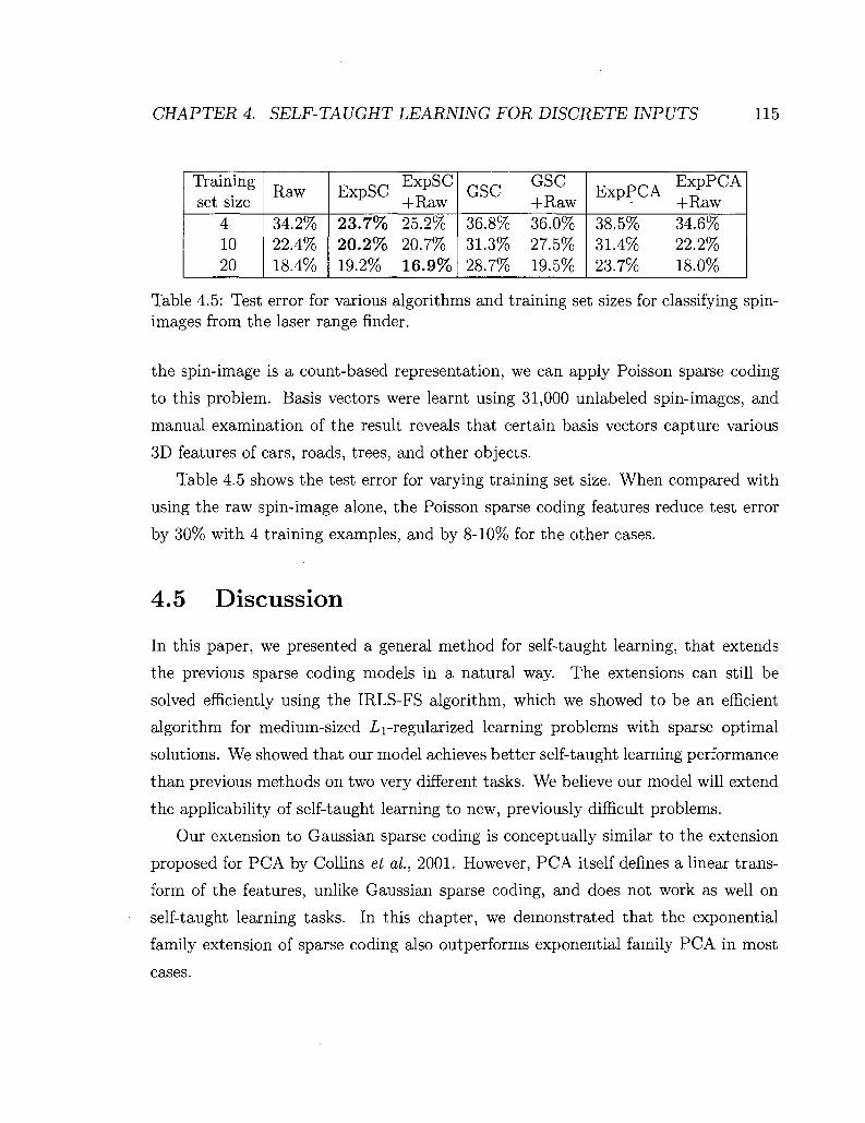
CHAPTER 4. SELF-TAUGHT LEARNING FOR DISCRETE INPUTS 115
Training set size
4 10 20
Raw
34.2% 22.4% 18.4%
ExpSC E ^ p S C
+Raw 23.7% 25.2% 20.2% 20.7% 19.2% 16.9%
GSC G ^ C
36.8% 36.0% 31.3% 27.5% 28.7% 19.5%
ExpPCA E xR
p P C A
+Raw 38.5% 34.6% 31.4% 22.2% 23.7% 18.0%
Table 4.5: Test error for various algorithms and training set sizes for classifying spin-images from the laser range finder.
the spin-image is a count-based representation, we can apply Poisson sparse coding
to this problem. Basis vectors were learnt using 31,000 unlabeled spin-images, and
manual examination of the result reveals that certain basis vectors capture various
3D features of cars, roads, trees, and other objects.
Table 4.5 shows the test error for varying training set size. When compared with
using the raw spin-image alone, the Poisson sparse coding features reduce test error
by 30% with 4 training examples, and by 8-10% for the other cases.
4.5 Discussion
In this paper, we presented a general method for self-taught learning, that extends
the previous sparse coding models in a natural way. The extensions can still be
solved efficiently using the IRLS-FS algorithm, which we showed to be an efficient
algorithm for medium-sized L\-regularized learning problems with sparse optimal
solutions. We showed that our model achieves better self-taught learning performance
than previous methods on two very different tasks. We believe our model will extend
the applicability of self-taught learning to new, previously difficult problems.
Our extension to Gaussian sparse coding is conceptually similar to the extension
proposed for PCA by Collins et al, 2001. However, PCA itself defines a linear trans
form of the features, unlike Gaussian sparse coding, and does not work as well on
self-taught learning tasks. In this chapter, we demonstrated that the exponential
family extension of sparse coding also outperforms exponential family PCA in most
cases.

CHAPTER 4. SELF-TAUGHT LEARNING FOR DISCRETE INPUTS 116
Compared to LDA, our model is more general because it can be applied to non
text and non-exchangeable domains. Further, it has been pointed out that when LDA
topics are viewed as defining a simplex over word distributions, the exact topics learnt
by LDA can vary a lot—the only constraint is that the simplex defined by the topics
still spans all the training documents (Blei et al., 2003). In our view, the additional
sparsity constraints in the sparse coding model help reduce this ambiguity, and allow
large numbers of "topics" to be learnt robustly.

Chapter 5
Large-scale Deep Unsupervised
Learning
In the first few chapters of this thesis, we have considered variants of the sparse cod
ing model for unsupervised learning of representations. In this chapter, we consider a
more general setting, where we are interested in learning not just a single layer of rep
resentation (obtained by the activations or features in our sparse coding algorithms),
but in multiple layers of representation, with each layer using the previous layer as
input to build successively more abstract concepts. Learning algorithms for multiple
layers of representation are often called "deep learning" algorithms.
In this chapter, we consider two well-known unsupervised learning models, deep
belief networks (DBNs) and sparse coding, that can learn hierarchical representations
of their input (Olshausen & Field, 1996b; Hinton & Salakhutdinov, 2006). With the
invention of increasingly efficient learning algorithms over the past decade, these
models have been applied to a number of machine learning applications, including
computer vision (Larochelle et al., 2007), text modeling (Salakhutdinov & Hinton,
2007) and collaborative filtering (Salakhutdinov et al., 2007), among others. We
have already discussed some such applications of sparse coding in previous chapters.
These models are especially well-suited to problems with high-dimensional inputs,
over which they can learn rich models with many latent variables or layers. When
applied to images, these models can easily have tens of millions of free parameters,
117

CHAPTER 5. LARGE-SCALE DEEP UNSUPERVISED LEARNING 118
and ideally, we would want to use millions of unlabeled training examples to richly
cover the input space. Unfortunately, with current algorithms, parameter learning at
this scale can take weeks using a conventional implementation on a single CPU. Partly
due to such daunting computational requirements, typical applications of DBNs and
sparse coding considered in the literature generally contain many fewer free parame
ters (e.g., see Table 5.1), or are trained on a fraction of the available input examples.
5.1 Deep learning algorithms
Many classical machine learning algorithms, such as support vector machines or lo
gistic regression, can be viewed as learning a single function h that transforms an
input vector x into the output label prediction y. In practice, the leap from the input
vector x to the abstract prediction y can be hard to achieve via a single function h.
For example, for image classification, these algorithms might have to learn a function
h that maps the pixel intensities x in an image directly to a prediction about whether
the image contains an elephant or not. Or, for text classifications, the algorithms
might learn a function that maps the raw words occuring in a document to a pre
diction about whether the document is a Sports document. Such applications often
use various hand-designed features to be computed on the inputs first, so that the
mapping from those features to the output label can be reasonably computed in a
single step. The learned function h is a single step of representation, and does not
capture composition of functions directly. Such algorithms that rely on a single step
(or layer) of representation are often called "shallow" learning algorithms.
In contrast, learning algorithms that attempt to learn a sequence of functions
hi, h2, . . . , /ifc, and then make a final prediction using the composition h(x) =
/ii(/i2(- • • hk(x))), do not need to learn everything about the input-to-label mapping
in a single step. Each composition can slowly abstract from low-level input dimen
sions, towards the high-level output label. Thus, for images, we could first learn to
detect edges from the pixels in an image, then we could use the edges to learn angles
and corners, till ultimately we can learn high-level concepts after several layers of
abstraction. To contrast these algorithms with shallow algorithms that learn a single

CHAPTER 5. LARGE-SCALE DEEP UNSUPERVISED LEARNING 119
layer of representation, such algorithms are often called "deep" learning algorithms.
Neural networks with multiple layers of representation are an example of a deep
learning algorithm (Rumelhart et al., 1987). However, supervised learning of deep
neural networks with many layers of representation is often prone to local minima,
and such networks are usually extremely difficult to train using only labeled data.
There has been significant recent work on deep learning algorithms, including the
development of several practical algorithms for learning deep models using unlabeled
data (Hinton & Salakhutdinov, 2006; Bengio et al., 2006). These algorithms are
based on learning the deep model a single layer at a time, by gaining a slightly more
abstract representation at each layer. Further, recent theoretical work demonstrates
that deep learning has significant theoretical advantages—loosely speaking, it can
be shown that there are learning problems for which a shallow learning algorithm
would require an exponential number of free parameters to be learned, but for which
a deep learning model might require only a linear number of free parameters (Bengio
& Lecun, 2007). Intuitively, shallow learning algorithms that attempt to capture the
label in one step are subject to a combinatorial problem of capturing all variations
in the input data, but deep learning algorithms can sometimes avoid these problems
by learning simple concepts first, and then combining these concepts to learn more
complex concepts.
We consider two specific algorithms for unsupervised learning of deep models,
deep belief networks (Hinton & Salakhutdinov, 2006) and sparse coding (Olshausen
& Field, 1996a), though many of our observations extend more generally to other
unsupervised learning algorithms for deep models, such the autoencoder-based algo
rithms for learning deep neural networks (Bengio et a l , 2006). In our view, the power
of deep learning algorithms can be best utilized when we can learn large, deep models
with many millions of parameters, and train such models using massive amounts of
unlabeled data. This requires that we consider algorithms for large-scale learning of
such deep models.

CHAPTER 5. LARGE-SCALE DEEP UNSUPERVISED LEARNING 120
5.2 Large-scale learning
Current learning algorithms for deep unsupervised learning methods, including DBNs
and sparse coding, are extremely slow for learning large models, or for learning with
large numbers of unlabeled examples. In our view, if the goal is to deploy better
machine learning applications, the difficulty of learning large models is a severe limi
tation. To take a specific case study, for two widely-studied statistical learning tasks
in natural language processing—language modeling and spelling correction—it has
been shown that simple, classical models can outperform newer, more complex mod
els, just because the simple models can be tractably learnt using orders of magnitude
more input data (Banko & Brill, 2001b; Banko & Brill, 2001a; Brants et al., 2007).
Analogously, in our view, scaling up existing DBN and sparse coding models to use
more parameters, or more training data, might produce very significant performance
benefits. For example, it has been shown that sparse coding exhibits a qualitatively
different and highly selective behavior called "end-stopping" when the model is large,
but not otherwise (Lee et al., 2007a). There has been a lot of recent work on scaling
up DBN and sparse coding algorithms, sometimes with entire research papers devoted
to ingenious methods devised specifically for each of these models (Hinton et al., 2006;
Bengio et al., 2006; Murray & Kreutz-Delgado, 2006; Lee et al., 2007a; Kavukcuoglu
et al., 2008). In our view, better self-taught learning performance can also be achieved
just by having the ability to train larger scale models, using larger numbers of training
examples.
Meanwhile, the raw clock speed of single CPUs has begun to hit a hardware power
limit, and most of the growth in processing power is increasingly obtained by throwing
together multiple CPU cores, instead of speeding up a single core (Gelsinger, 2001;
Frank, 2002). Recent work has shown that several popular learning algorithms such
as logistic regression, linear SVMs and others can be easily implemented in parallel
on multicore architectures, by having each core perform the required computations
for a subset of input examples, and then combining the results centrally (Dean &
Ghemawat, 2004; Chu et al., 2006). However, standard algorithms for DBNs and
sparse coding are difficult to parallelize with such "data-parallel" schemes, because

CHAPTER 5. LARGE-SCALE DEEP UNSUPERVISED LEARNING 121
Published source Hinton et al., 2006 Hinton & Salakhutdinov, 2006 Salakhutdinov k Hinton, 2007 Ranzato & Szummer, 2008
Application Digit images Face images Semantic hashing Text
Our model
#Params 1.6mn 3.8mn 2.6mn 3mn lOOmn
Table 5.1: A rough estimate of the number of free parameters (in millions) in some recent deep belief network applications reported in the literature, compared to our desired model. To pick the applications, we looked through several research papers and picked the ones for which we could reliably tell the number of parameters in the model. AH the models do not implement exactly the same algorithm, and the applications cited may not have used the largest-scale models possible, so this is not an exact comparison; but the order of magnitude difference between our desired model and recent work is striking.
they involve iterative, stochastic parameter updates, such that any update depends
on the previous updates. This makes the updates hard to massively parallelize at a
coarse, data-parallel level (e.g., by computing the updates in parallel and summing
them together centrally) without losing the critical stochastic nature of the updates.
It appears that fine-grained parallelism might be needed to successfully parallelize
these tasks.
In this chapter, we exploit the power of modern graphics processors (GPUs) to
tractably learn large DBN and sparse coding models. The typical graphics card
shipped with current desktops contains over a hundred processing cores, and has a
peak memory bandwidth several times higher than modern CPUs. The hardware
can work concurrently with thousands of threads at any time, and is able to schedule
these threads on the available cores with very little overhead. Such fine-grained paral
lelism makes graphics processors (GPUs) increasingly attractive for general-purpose
computation that is hard to parallelize on other distributed architectures.
There is of course a tradeoff—this parallelism is obtained by devoting many more
transistors to data processing, rather than to caching and control flow operations,
as in a regular CPU core. This puts specific constraints on the types of instruc
tions and memory accesses that can be efficiently implemented (discussed further in
Section 5.3). Thus, the main challenge in successfully applying GPUs to a machine

CHAPTER 5. LARGE-SCALE DEEP UNSUPERVISED LEARNING 122
30 MPs
Shared Memory
(16K)
SP
SP
SP
SP
SP
SP
SP
SP
100GB/S < > (coalesced)-^-
Global Memory (1GB)
Figure 5.1: Simplified schematic for the Nvidia GeForce GTX 280 graphics card, with 240 total cores (30 multiprocessors with 8 stream processors each).
learning task is to redesign the learning algorithms to meet these constraints as far as
possible. While a thorough introduction to graphics processor architecture is beyond
the scope of this thesis, we now review the basic ideas behind successful computation
with GPUs.
5.3 Computing with graphics processors
We illustrate the principles of GPU computing using Nvidia's CUDA programming
model (Harris, 2008). Figure 5.1 shows a simplified schematic of a typical Nvidia
GPU. The GPU hardware provides two levels of parallelism: there are several multi
processors (MPs), and each multiprocessor contains several stream processors (SPs)
that run the actual computation. The computation is organized into groups of
threads, called "blocks", such that each block is scheduled to run on a multipro
cessor, and within a multiprocessor, each thread is scheduled to run on a stream
processor.
All threads within a block (and thus executing on the same multiprocessor) have
1000 GB/s
MPi
Shared Memory
(16K)
><
>< SP
SP
SP
SP
>
> SP
SP
SP
SP
MP2
Shared Memory
(16K)
J SP]|SP11SP|[SP
SP]|SP1ISP1[SP

CHAPTER 5. LARGE-SCALE DEEP UNSUPERVISED LEARNING 123
shared access to a small amount (16 KB) of very fast "shared memory," and they
can synchronize with each other at different points in their execution. All threads
also have access to a much larger GPU-wide "global memory" (currently up to 4
GB) which is slower than the shared memory, but is optimized for certain types
of simultaneous access patterns called "coalesced" accesses. Briefly, memory access
requests from threads in a block are said to be coalesced if the threads access memory
in sequence (i.e., the fc-th thread accesses the A;-th consecutive location in memory).1
When memory accesses are coalesced, the hardware can perform them in parallel for
all stream processors, and the effective access speed (between the stream processors
and the global memory) is several times faster than the access speed between a CPU
and RAM.
Since GPU computation and within-GPU memory accesses themselves are highly
parallel, in many algorithms, the main bottleneck arises in transferring data between
RAM and the GPU's global memory. For example, the total time taken to multiply
two 1000x1000 matrices using our GPU configuration (and a vendor-supplied linear
algebra package) is roughly 20 milliseconds, but the actual computation takes only
0.5% of that time, with the remaining time being used for transfer in and out of global
memory. A partial solution is to perform memory transfers only in large batches,
grouped over several computations. In our example, if we were doing 25 different
matrix multiplications and were able to perform memory transfers in large chunks
(by transferring all inputs together, and transferring all outputs together), then as
much as 25% of the total time is spent in computation. Thus, efficient use of the
GPU's parallelism requires careful consideration of the data flow in the application.
^ o r simplicity, we ignore certain other technical conditions that are easy to obey in practice. We also omit discussion of two other types of memory—constant and texture memory—that are optimized for other specific types of access patterns that we do not use in our applications.

CHAPTER 5. LARGE-SCALE DEEP UNSUPERVISED LEARNING 124
5.4 Preliminaries
We consider an unsupervised learning task where we are given a large unlabeled
dataset {x^\x^2\ . . . , x ^ } , where each input x^ £ Mn.2 The goal is to learn a model
for the inputs x, and to subsequently apply the model to specific machine learning
tasks (as in a self-taught learning setup). For example, each unlabeled input x^ E
M900 might represent a 30x30 pixel image of a handwritten character (represented as
a vector of pixel intensities). We might want to learn a model for the complex 900-
dimensional space of inputs, and then use this model for classifying new handwritten
characters using only very little labeled data.
5.4.1 Deep Belief Networks
DBNs are multilayer neural network models that learn hierarchical representations
for their input data. Hinton et al. (2006) proposed an unsupervised algorithm for
learning DBNs, in which the DBN is greedily built up layer-by-layer, starting from
the input data. Each layer is learnt using a probabilistic model called a restricted
Boltzmann machine (RBM). Briefly, an RBM contains a set of stochastic hidden units
h that are fully connected in an undirected model to a set of stochastic visible units
x. Assuming binary-valued units, the RBM defines the following joint distribution:
P(x,h) oc exp 2_]XiWijhj + V^CiXi + YJbjhj \ i,j i J J
where the weights w and biases b and c are parameters to be tuned. The condi
tional distributions can be analytically computed:
2For simplicity, we drop the subscript u in our previous notation x« for unlabeled examples, and represent unlabeled examples just as i'*' in this chapter.

CHAPTER 5. LARGE-SCALE DEEP UNSUPERVISED LEARNING 125
P(hj\x) = sigmoid(bj + / jw^Xj) (5.1) i
P{xi\h) = sigmoid(ci +^2 Wijhj) (5.2) i
Maximum likelihood parameter learning for an RBM can be efficiently approx
imated by contrastive divergence updates (Hinton, 2002), where we start with the
unlabeled examples as the visible units, alternately sample the hidden units h and
visible units x using Gibbs sampling (Equations 5.1-5.2), and update the parameters
as:
Wtj := Wij + 7? ( ( ^ j ) d a t a - ( z^ j ) s ample ) (5 .3)
C% '•= Ci + TJ ((Xj)data — (^i/sample) (5-4)
fy '•= bj + ? 7 ( ( / i j ) d a t a - ( ^ s a m p l e ) (5-5)
where r\ is the learning rate, (-)data represents expectations with the visible units
tied to the input examples, and ( sample represents expectations after T > 1 iteration's
of Gibbs sampling. Since each update requires a Gibbs sampling operation, and the
updates have to be applied over many unlabeled examples to reach convergence, un
supervised learning of the parameters can take several days to complete on a modern
CPU.
5.4.2 Sparse Coding
We briefly revisit the sparse coding model introduced in Chapter 3. Sparse coding
is an algorithm for constructing succinct representations of input data (Olshausen
& Field, 1996b). Using our earlier example, if each input x ^ e M900 represents a
handwritten character image, sparse coding attempts to learn that each handwritten
character is composed of only a few building blocks, such as pen strokes (instead of
900 arbitrary intensity values).

CHAPTER 5. LARGE-SCALE DEEP UNSUPERVISED LEARNING 126
Specifically, given inputs x £ K™, sparse coding attempts to find basis vectors
b = {&i, &2> • • • > &s}> fy G M.n such that each input x can be represented as a linear
combination of a few basis vectors: x ~ YljCijbj, where a,j € K represents the ac
tivation of basis bj, and most of the a,- values are zero (or, the vector a is sparse).
The basis vectors are found by solving the following optimization problem (Lee et al.,
2007a):
minimize^ \ £ \ \\x® - £V afbjf + 0 Ylij l«5°l
s.t. ||6j|| < 1, V?e{ l , . . . , s }
where the first term in the objective function encourages good reconstruction (x^ ~
^2jbjOj ) , and the second term encourages sparsity by penalizing non-zero activa
tions (Tibshirani, 1996a). The optimization problem is not jointly convex in both
b and a variables, but it is convex in either one of those variables, if the other is
kept fixed. In Chapter 2, we discussed an alternating minimization algorithm which
iterates over two steps: first, keeping b fixed, we optimize over a, which leads to
an Li-regularized least squares problem, that can be solved using custom-designed
solvers (Efron et al., 2004; Lee et a l , 2007a; Andrew & Gao, 2007). Then, we keep a
fixed, and optimize over b using convex optimization techniques (Lee et al., 2007a).
For problems with high-dimensional inputs and large numbers of basis vectors, the
first step is particularly time consuming as it involves a non-differentiable objective
function, and the overall learning algorithm can take several days.
5.5 GPUs for unsupervised learning
Both the above algorithms repeatedly execute the following computations: pick a
small number of unlabeled examples, compute an update (by contrastive divergence
or by solving a convex optimization problem), and apply it to the parameters. To
successfully apply GPUs to such unsupervised learning algorithms, we need to satisfy
two major requirements. First, memory transfers between RAM and the GPU's global
memory need to be minimized, or grouped into large chunks. For machine learning

CHAPTER 5. LARGE-SCALE DEEP UNSUPERVISED LEARNING 127
applications, we can achieve this by storing all parameters permanently in GPU
global memory during learning. Unlabeled examples usually cannot all be stored in
global memory, but they should be transferred only occasionally into global memory
in as large chunks as possible. With both parameters and unlabeled examples in
GPU global memory, the updates can be computed without any memory transfer
operations, with any intermediate computations also stored in global memory.
A second requirement is that the learning updates should be implemented to fit
the two level hierarchy of blocks and threads, in such a way that shared memory can
be used where possible, and global memory accesses can be coalesced. Often, blocks
can exploit data parallelism (e.g., each block can work on a separate input example),
while threads can exploit more fine-grained parallelism because they have access to
very fast shared memory and can be synchronized (e.g., each thread can work on a
single coordinate of the input example assigned to the block). Further, the graphics
hardware can hide memory latencies for blocks waiting on global memory accesses
by scheduling a ready-to-run block in that time. To fully use such latency hiding,
it is beneficial to use a large number of independently executing blocks. In some
cases, as discussed for sparse coding in Section 5.7, we might benefit from completely
redesigning the updates to be inherently parallel and requiring less synchronization
between threads.
Using these principles, we arrive at the following template algorithm for applying
GPUs to unsupervised learning tasks:
Algorithm 5 Parallel unsupervised learning on GPUs Initialize parameters in global memory. while convergence criterion is not satisfied do
Periodically transfer a large number of unlabeled examples into global memory. Pick a few of the unlabeled examples at a time, and compute the updates in parallel using the GPU's two-level parallelism (blocks and threads).
end while Transfer learnt parameters from global memory.

CHAPTER 5. LARGE-SCALE DEEP UNSUPERVISED LEARNING 128
5.6 Learning large deep belief networks
We apply Algorithm 5 to learning large DBNs using the contrastive divergence up
dates in Equations (5.3-5.5). The parameters w, c and b for all the DBN layers
are maintained permanently in global memory during training. The updates require
repeated Gibbs sampling using the distributions in Equations (5.1-5.2). These distri
butions can be rewritten using matrix notation:
P(h\x) = vectorSigmoid(6 + wTx)
P(x\h) — vectorSigmoid(c + wh)
where vectorSigmoid(-) represents the elementwise sigmoid function, and x, h
are vectors containing an element corresponding to each visible and hidden unit re
spectively. The above computations can be batched together for several examples for
further efficiency. The matrix operations can be performed in parallel using optimized
linear algebra packages for the GPU, and the sigmoid computation and sampling can
be done by a simple parallelization scheme where each block works on a single exam
ple, and each thread in the block works on a single element of the example. Finally,
once the samples have been generated, the updates can again be applied in parallel
using linear algebra packages: e.g., w := w + rj ((xTh)data, - (xTh)sa,mpie)
We extend our method to learning deep belief networks with "overlapping patches"
as shown in Figure 5.2. This model is most easily understood with hidden and visible
units arranged in a 2-D array (e.g., when the input is an image and each visible unit
is a pixel). The input image is fully tiled by equally-spaced, equal-sized patches (or
receptive fields), and each patch is fully connected to a unique group of hidden units.
There is no sharing of weights in this model, and each connection is parameterized
by a free parameter. Each group of hidden units is connected only to a local window
(or patch, or receptive field) of visible units, with each connection parameterized by
a free parameter (and no weight sharing). Because of the overlapping patches, all the
parameters in the model depend on each other, making learning hard. However, Gibbs

CHAPTER 5. LARGE-SCALE DEEP UNSUPERVISED LEARNING 129
Figure 5.2: A schematic diagram of the overlapping patches model for deep belief networks. Two patches A and B in the input image are shown, with each patch connected to a different set of hidden units. The connections are parameterized by their own sets of parameters u^, &A, CA and wB, bB,CB-
sampling can still be performed in parallel for this model: each visible unit depends
on hidden units at many different locations, but the sampling operation x\h can be
implemented using only coalesced global memory accesses (implementation details:
this can be achieved by using the shared memory available in graphics processors, as
shared memory accesses do not need to be coalesced for efficient access). The upward
sampling operation h\x still uses a local patch of pixels, and can be implemented
using coalesced accesses. Finally, once the sampling operations are performed, weight
updates can be applied by considering the cross products Xihj in the samples, and
this can be done efficiently in parallel as well.
These overlapping patch RBMs can be stacked on top of each other, such that the
second-layer RBM contains hidden units connected locally to first-layer hidden units,
and so on. The resulting deep networks have a very large number of units, but only
sparse, local connections, which make learning tractable even for models with more
than 100 million parameters.

CHAPTER 5. LARGE-SCALE DEEP UNSUPERVISED LEARNING 130
5.6.1 Experimental Results
We compare our GPU-based algorithm against CPU-based methods using the follow
ing multicore hardware:
• GPU: Nvidia GeForce GTX 280 graphics card with 1GB memory. The machine
had a dual-core CPU @ 3.16GHz. The reported running time results show the
total running time (including all computation, memory transfer, etc.).
• Single CPU: Single core @ 3.16GHz.
• Dual-core CPU: Two cores, each @ 3.16GHz. (Identical machine as for the
GPU result.)
• Quad-core* CPU: Four cores, each @ 2.40GHz.3
The CPU-based method was implemented using two highly optimized multi
threaded linear algebra packages: ATLAS BLAS (Whaley et al., 2001) and Goto
BLAS (Goto & van de Geijn, 2007). Consistent with previous results, we found that
Goto BLAS was faster (Bengio, 2007), so we report CPU results using it. As input,
we used a large dataset of natural images (van Hateren & van der Schaaf, 1998)
and obtained input examples by randomly extracting square image patches of the
required size. Following previous work, we used Gaussian visible units and binary
hidden units, and trained a sparse RBM by adding an additional penalty term to the
objective (Lee et al., 2007b)—however, these modifications do not affect the running
time results significantly. For learning, we performed one-step contrastive divergence
updates using a mini-batch of 192 examples.
Table 5.2 shows the running time for processing 1 million examples for RBMs of
varying size (denoted by number of visible units x number of hidden units). The
GPU method is between 12 to 72 times faster. The speedup obtained is highest
for large RBMs, where the computations involve large matrices and can be more
3Note that each core in our quad-core machine is somewhat slower than the single CPU core, so that the peak processing power of the quad-core is a little more than three times that of the single CPU. For this reason, the quad-core machine does not always perform better than the single/dual-core machine. We put an asterisk on quad-core* everywhere to remind the reader of this distinction.
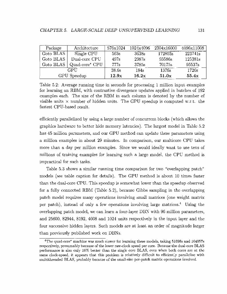
CHAPTER 5. LARGE-SCALE DEEP UNSUPERVISED LEARNING 131
Package Goto BLAS Goto BLAS Goto BLAS
Architecture Single CPU
Dual-core CPU Quad-core* CPU
GPU GPU Speedup
576x1024 1024x4096 2304x16000 4096x11008 563s 3638s 172803s 223741s 497s 2987s 93586s 125381s 777s 3785s 70175s 95537s 38.6s 184s 1376s 1726s 12.9x 16.2x 51.0x 55.4x
Table 5.2: Average running time in seconds for processing 1 million input examples for learning an RBM, with contrastive divergence updates applied in batches of 192 examples each. The size of the RBM in each column is denoted by the number of visible units x number of hidden units. The GPU speedup is computed w.r.t. the fastest CPU-based result.
efficiently parallelized by using a large number of concurrent blocks (which allows the
graphics hardware to better hide memory latencies). The largest model in Table 5.2
has 45 million parameters, and our GPU method can update these parameters using
a million examples in about 29 minutes. In comparison, our multicore CPU takes
more than a day per million examples. Since we would ideally want to use tens of
millions of training examples for learning such a large model, the CPU method is
impractical for such tasks.
Table 5.3 shows a similar running time comparison for two "overlapping patch"
models (see table caption for details). The GPU method is about 10 times faster
than the dual-core CPU. This speedup is somewhat lower than the speedup observed
for a fully connected RBM (Table 5.2), because Gibbs sampling in the overlapping
patch model requires many operations involving small matrices (one weight matrix
per patch), instead of only a few operations involving large matrices.4 Using the
overlapping patch model, we can learn a four-layer DBN with 96 million parameters,
and 25600, 82944, 8192, 4608 and 1024 units respectively in the input layer and the
four successive hidden layers. Such models are at least an order of magnitude larger
than previously published work on DBNs. 4The quad-core* machine was much slower for learning these models, taking 51698s and 104057s
respectively, presumably because of the lower raw-clock speed per core. Because the dual-core BLAS performance is also only 16% better than the single core BLAS, even when both cores are at the same clock-speed, it appears that this problem is relatively difficult to efficiently parallelize with multithreaded BLAS, probably because of the small-size per-patch matrix operations involved.

CHAPTER 5. LARGE-SCALE DEEP UNSUPERVISED LEARNING 132
Packag Goto Goto
s Arch. Single CPU Dual-core
GPU GPU Speedup
20736x4915236864x92928 38455s 77246s 32236s 65235s 3415s 6435s 9.4x 10. lx
Table 5.3: Average time in seconds for processing 1 million examples for the overlapping patch model, with contrastive divergence updates applied in batches of 192 examples each. The model size in each column is denoted by the number of visible units x number of hidden units (but note that the units are not fully connected). The two models were created by taking 144x144 pixel and 192x192 pixel inputs respectively; the size of each patch is 24x24 pixels, there are 192 hidden units connected to each patch, and neighboring patches are 8 pixels apart. Overall, the models have 28 million and 54 million free parameters respectively.
Finally, we note that the overlapping patches model can be modified to share pa
rameters in all patches, such that, for example, U>A = WB m Figure 5.2. If overlapping
patches are tiled one pixel apart, this model is identical to the convolutional RBM
model (Desjardins & Bengio, 2008; Lee et al., 2009a). Contrastive divergence learning
in this model can be implemented by using convolutions to perform the Gibbs sam
pling operation h\x. For small to medium filter (patch) sizes, spatial convolution can
be implemented very efficiently using GPUs, by having each block read a filter into
shared memory, then reading the input image column-by-column into shared mem
ory, and finally aggregating the output elements affected by that filter and that input
image column. It can be shown that by ordering operations in this way, we use only
fast shared memory accesses and coalesced global memory accesses.5 For example, on
computing the convolution of 32 128x128 images with 32 16x16 filters, our GPU im
plementation of spatial convolution (including the time to transfer images/filters into
GPU memory) is over 100 times faster than either spatial convolution implemented
in C or FFT-based convolution in Matlab.
5For larger filter sizes FFT-based convolution is generally better, and a GPU FFT package can be used.

CHAPTER 5. LARGE-SCALE DEEP UNSUPERVISED LEARNING 133
5.7 Parallel sparse coding
We now consider the sparse coding optimization problem discussed in Section 5.4.2.
Following the template in Algorithm 5, we maintain the basis parameters b perma
nently in global memory, and transfer input examples to GPU global memory period
ically in large batches. Following the alternating minimization method, each update
itself consists of two steps: the first, simpler part of the update involves optimizing
over b, given fixed a. This leads to the following constrained optimization problem:
minimize £ . \\x® - £ \ afbjf s.t. \\bjW < 1, Vj
We solve this problem using projected gradient descent, where we follow the gra
dient of the quadratic objective function, and project at each step to the feasible set.6
This method is guaranteed to converge to the optimal b and can be straightforwardly
implemented using a GPU linear algebra package.
The other part of the update involves optimizing over a, given fixed b. Since the
activation a^ for each example x® is now independent of the activations for other
examples, it suffices to consider the following canonical Li-regularized least squares
problem for a single input example x:
minimize a \\\x - ^ - cijbj\\2 + PJ2j \aj\ (5-6)
The objective function is not differentiable because of the Lx-penalty term. This
problem has recently received wide attention because of its robust feature selection
properties (Tibshirani, 1996a; Ng, 2004), and several custom algorithms have been
designed to solve it (Efron et al., 2004; Lee et a l , 2007a; Andrew & Gao, 2007).
Some of these algorithms use sparse linear algebra operations to achieve efficiency.
We instead present a very different two-stage algorithm that is inherently parallel,
6The projection operation is particularly simple: for each basis vector bj, if ||6j|| > 1 then rescale bj to have norm 1, otherwise keep bj unchanged.
CHAPTER 5. LARGE-SCALE DEEP UNSUPERVISED LEARNING 134
and is thus able to use the GPU hardware more efficiently.
5.7.1 Parallel Li-regularized least squares
Our algorithm is based on the observation that in the optimization problem in Equa
tion (5.6), if we vary only one of the activations a,j, while keeping the other activations
fixed, the optimal value a* can be easily computed (Friedman et al., 2007). Letting
B be a matrix with bj as its j-th. column, and r^ = bjbj:
if \gj -rj-ajl < P
if g6 - rjdj > (5
if gj - rfy < -P
BTBa - BTx.
The updates can be efficiently performed in parallel by having thread j compute
just one coordinate a*. Further, since we usually batch several examples together, we
can precompute the matrix BTB, the vector BTx and the vector r once in parallel,
store the result in global memory, and perform only efficient accesses to compute all
a*j values.7
Thus, we propose the following iterative algorithm: at each iteration, starting at
the current activation values a = a, we compute all the optimal coordinate values a*j
in parallel as outlined above. Then, we perform a line search in the direction of vector
d = a* — a. The line search consists of finding a step size t > 0 such that the value of
the objective function at the point a = a + td is lower than the value at a = a. This
line search, including the function evaluations, can be run in parallel.8 We then move
7To see why, note that to compute a*, thread j needs to compute gj — r^j = ^Zt(BTB)tjat —
(BTx)j — rjCbj. Consider the elements thread j accesses: (i) (BTB)tf Accesses can be coalesced if BTB is stored in row-major order, (ii) By maintaining a in shared memory, all threads can access the same element at simultaneously, as well as access the elements a,j that are different for each thread. (For the interested reader, we add that this avoids "bank conflicts" in shared memory. See CUDA reference manual for details.) (iii) (BTx)j and ry. Can be coalesced as thread j accesses the j - th location.
8Details: By substituting a = a + td in the original objective function, the line search reduces
a: =
0
(~9j + rjaj + P)IT3
(~9j + r^j - P)/rj
1 where fir = Va -\\x - ^ % ^ | | 2 =

CHAPTER 5. LARGE-SCALE DEEP UNSUPERVISED LEARNING 135
Method Single CPU Dual-core GPU Speedup
Sparsity«3% 6% 10% 215s 403s 908s 191s 375s 854s 37.0s 41.5s 55.8s 5.2x 9.0x 15.3x
Table 5.4: Average running time for updating sparse coding parameters on 5000 input examples. The GPU speedup is computed w.r.t. the fastest CPU-based result. Lee et al.'s algorithm appears to be difficult to parallelize using multithreaded Matlab, because it is an active set method that performs only small matrix operations (including inverses) most of the time. The sparsity value refers to the average percentage of the 1024 activations that were nonzero at the optimal solution. Note that 3-10% is a reasonable range as it corresponds to around 30 to 100 nonzero activations per input example.
to the new point a = a + td, and iterate. We declare convergence when the objective
value decreases by less than a 10~6 fraction of the previous objective value.
Since the direction d is a nonnegative linear combination of descent directions
along the coordinate axes: dj = a* — a,j, d must itself be a descent direction for the
objective function. Thus, at each iteration, a step size t > 0 can always be found that
reduces the value of the objective function, and the overall algorithm is guaranteed
to converge to the optimal solution.
This algorithm uses fine-grained parallelism by having each thread compute just
one coordinate of the solution. Such highly multithreaded execution is especially
well-suited for graphics processors, as the hardware is able to hide memory latency
(for threads blocked on memory accesses) by scheduling other threads that are not
blocked on memory accesses, and leads to high utilization of the available cores.
5.7.2 Experimental Results
We again compare our method against a multicore CPU baseline (Lee et al., 2007a).
We used optimized Matlab code provided by Lee et al. For the CPU multicore results,
we executed Matlab with multithreading enabled. Since different choices for the
to minimizing a 1-D function of the form /(£) = a%t2 + a,\t + ao + j3\\a + td\\i, where the values a2,ai,ao can be computed in parallel. For the 1-D line search over /(£), we simply try a fixed set of positive step sizes, and pick the largest step size that reduces the value of the objective function.
CHAPTER 5. LARGE-SCALE DEEP UNSUPERVISED LEARNING 136
regularization parameter j3 produce solutions of different sparsity, we experimented
with a range of choices.
Table 5.4 shows the running time9 for applying sparse coding basis updates (in
cluding both basis and activation optimization) for k = 5000 examples, with mini-
batches of 1000 examples. Each example x E R1024 was obtained via a randomly
sampled 32x32 pixel natural image patch. We used s = 1024 basis vectors, initialized
randomly. The large majority of sparse coding time in Lee et al.'s method is taken
by the activation learning step, especially when many activations are nonzero at the
optimum. By effectively parallelizing this step, our GPU method is up to 15 times
faster than a dual-core implementation.
We note that in our self-taught learning algorithm, the basis learning can be done
offline (before we see any test examples), but activations need to be computed for
every new example that we wish to classify. This means that it is especially important
that the activation learning procedure be very efficient, as it is used at classification
time. When compared just as a method for computing activations (and not in the
alternating procedure for basis learning), our GPU method is up to 27 times faster
than the CPU baseline.
5.8 Discussion
Graphics processors are able to exploit finer-grained parallelism than current multi-
core architectures or distributed clusters. They are designed to maintain thousands of
active threads at any time, and to schedule the threads on hundreds of cores with very
low scheduling overhead. The map-reduce framework (Dean & Ghemawat, 2004) has
been successfully applied to parallelize a class of machine learning algorithms (Chu
et al., 2006). However, that method relies exclusively on data parallelism—each core
might work independently on a different set of input examples—with no further sub
division of work. In contrast, the two-level parallelism offered by GPUs is much more
powerful: the top-level GPU blocks can already exploit data parallelism, and GPU
9The quad-core* machine was slower than the dual-core machine for these models, taking 271s, 574s and 1441s respectively, because of the lower raw-clock speed per core.
CHAPTER 5. LARGE-SCALE DEEP UNSUPERVISED LEARNING 137
threads can further subdivide the work in each block, often working with just a single
element of an input example.
We note that GPUs have been applied to certain problems in machine learning,
including SVMs (Catanzaro et al., 2008), and to supervised learning in convolutional
networks (Chellapilla et al., 2006). A general map-reduce framework for GPUs has
also been developed (He et al., 2008), but it usually gives lower performance than
a customized GPU method. We hope that our experiments will encourage large-
scale applications of deep belief networks and sparse coding to self-taught learning
problems. XXX.

Chapter 6
Conclusions
Self-taught learning is a new framework for using unlabeled data in supervised clas
sification tasks. This framework does not require that the unlabeled data follow the
class labels of the supervised task, or arise from the same generative distribution.
Such unlabeled data is often significantly easier to obtain than in previously studied
frameworks such as semi-supervised learning. In this thesis, we have demonstrated
that self-taught learning can be applied successfully to a variety of hard machine
learning problems.
Algorithms for self-taught learning: The centerpiece of our work is a self-
taught learning algorithm based on an optimization problem called "sparse coding."
This algorithm uses unlabeled data to learn a new representation for complex, high-
dimensional inputs, and then applies supervised learning over this representation.
The representation captures higher-level aspects of the input, and significantly im
proves classification performance on many test domains, including computer vision,
audio recognition and text classification (Raina et al., 2007). We have also developed
efficient sparse coding algorithms for a translation-invariant version of the model,
that can be applied to audio and image data (Grosse et al., 2007). We also generalize
the model to a much broader class of inputs (the exponential family of distributions),
and apply the model to text classification and a robotic perception task (Lee et al.,
2009b). Taken together, these experiments demonstrate that machine learning can
be applied to much harder problems than previously possible.
138

CHAPTER 6. CONCLUSIONS 139
Large-scale algorithms: These self-taught learning algorithms work best when
they are allowed to learn rich models (with millions of parameters) using large amounts
of unlabeled data (millions of examples). Unfortunately, with current methods, it can
take weeks to learn such rich models. Further, these methods require fast, sequen
tial updates, and with current algorithms, are not conducive to being parallelized
on a distributed cluster, such as the commonly used map-reduce cluster. To apply
self-taught learning to such large-scale problems, we show that graphics processor
hardware (available in most modern desktops) can be used to massively parallelize
the algorithms. Using a new inherently parallel algorithm, the sparse coding algo
rithm can be easily implemented on graphics processors, and we show that this can
reduce the learning time from about three weeks to a single day (Raina et al., 2009).
Learning hierarchical representations: Finally, we consider self-taught learn
ing methods that learn hierarchical representations using unlabeled data. We focus
on a particular hierarchical model, the deep belief network, that has received wide
attention in the machine learning community in recent years. We develop general
principles for unsupervised learning of such hierarchical models using graphics pro
cessors, and show that the slow learning algorithms for deep belief networks can be
successfully parallelized. This implementation is up to 70 times faster than an op
timized CPU implementation, reduces the learning time from weeks to hours, and
represents the state-of-the-art in learning deep belief networks (Raina & Ng, 2008).
Learning for the Internet age: The last decade has been characterized by a
veritable explosion in the amount of data freely available. It is now possible to almost
routinely obtain hundreds of millions of images, or even billions of English documents
on the Web. Websites such as Google and Facebook serve billions of webpages every
month. Developing machine learning algorithms that can operate at these scales is a
challenge.
Further, since a large proportion of the available data is unlabeled, progress in
machine learning might well rely on the development of unsupervised learning algo
rithms that can use large amounts of unlabeled data. In this thesis work, we show
that unlabeled data can be used profitably in a variety of applications—the algo
rithms we describe are almost completely unsupervised, but can perform remarkably

CHAPTER 6. CONCLUSIONS 140
well on image, text and audio data. However, we believe that this work is still just
scraping the surface of possibilities, and the potential benefits of using easily available
unlabeled data can be truly enormous.

Bibliography
(2005). A sparse texture representation using local affine regions. IEEE Trans. Pattern
Anal. Mach. Intell, 27, 1265-1278. Lazebnik, Svetlana and Schmid, Cordelia and
Ponce, Jean.
Ando, R. K., & Zhang, T. (2005). A framework for learning predictive structures
from multiple tasks and unlabeled data. Journal of Machine Learning Research, 6,
1817-1853.
Andrew, G., & Gao, J. (2007). Scalable training of Li-regularized log-linear models.
ICML.
Atick, J. (1992). Could information theory provide an ecological theory of sensory
processing. Network: Computation in Neural Systems, 3, 213-251.
Banko, M., & Brill, E. (2001a). Mitigating the paucity-of-data problem: exploring
the effect of training corpus size on classifier performance for natural language
processing. First international conference on Human language technology research
(pp. 1-5).
Banko, M., & Brill, E. (2001b). Scaling to very very large corpora for natural language
disambiguation. ACL.
Baxter, J. (1995). Learning internal representations. COLT. Santa Cruz, California,
United States.
Baxter, J. (1997). Theoretical models of learning to learn. In T. Mitchell and S. Thrun
(Eds.), Learning to learn.
141

BIBLIOGRAPHY 142
Belkin, M., Niyogi, P., & Sindhwani, V. (2005). On Manifold Regularization. AISTAT.
Bell, A. J., & Sejnowski, T. J. (1995). An information-maximization approach to
blind separation and blind deconvolution. Neural Computation, 7, 1129-1159.
Belongie, S., Malik, J., & Puzicha, J. (2002). Shape matching and object recognition
using shape contexts. IEEE Trans. Pattern Anal. Mack. Intell, 24, 509-522.
Ben-David, S., Lu, T., & Pal, D. (2008). Does unlabeled data provably help? worst-
case analysis of the sample complexity of semi-supervised learning. COLT (pp.
33-44).
Ben-David, S., & Schuller, R. (2003). Exploiting task relatedness for multiple task
learning. COLT.
Bengio, Y. (2007). Speeding up stochastic gradient descent. NIPS Workshop on
Efficient Machine Learning.
Bengio, Y., Lamblin, P., Popovici, D., & Larochelle, H. (2006). Greedy layer-wise
training of deep networks. NIPS.
Bengio, Y., & Lecun, Y. (2007). Scaling learning algorithms towards ai MIT Press.
Berg, A., Berg, T., k, Malik, J. (2005). Shape matching and object recognition using
low distortion correspondence. CVPR.
Bishop, C. (1995). Neural networks for pattern recognition. Oxford University Press.
Bishop, C. M. (2006). Pattern recognition and machine learning. Springer.
Blei, D., Ng, A. Y., k Jordan, M. (2002). Latent Dirichlet allocation. NIPS.
Blei, D., Ng, A. Y., & Jordan, M. I. (2003). Latent Dirichlet allocation. JMLR, 3,
993-1022.
Blum, A., & Chawla, S. (2001). Learning from labeled and unlabeled data using
graph mincuts. ICML (pp. 19-26). Morgan Kaufmann Publishers Inc.

BIBLIOGRAPHY 143
Blumensath, T., & Davies, M. (2006). Sparse and shift-invariant representations of
music. IEEE Transactions on Audio, Speech, and Language Processing (pp. 50-57).
Boyd, S., & Vandenberghe, L. (2004). Convex optimization. Cambridge University
Press.
Boynton, G., & Hegde, J. (2004). Visual cortex: The continuing puzzles of area v2.
Current Biology, U, 523R-524R.
Bradley, D., & Bagnell, J. A. (2008). Differentiate sparse coding. NIPS.
Brants, T., Popat, A. C , Xu, P., Och, F. J., & Dean, J. (2007). Large language
models in machine translation. EMNLP-CoNLL.
Caruana, R. (1997). Multitask learning. Machine Learning, 28, 41-75.
Catanzaro, B. C , Sundaram, N., & Keutzer, K. (2008). Fast support vector machine
training and classification on graphics processors. ICML.
Cavanaugh, J., Bair, W., & Movshon, J. (2002). Nature and interaction of signals
from the receptive field center and surround in macaque vl neurons. Journal of
Neurophysiology, 88, 2530-2546.
Chapelle, O., Scholkopf, B., & Zien, A. (Eds.). (2006). Semi-supervised learning.
Cambridge, MA: MIT Press.
Chellapilla, K., Puri, S., & Simard, P. (2006). High performance convolutional neural
networks for document processing. Frontiers in Handwriting Recognition.
Chu, C. T., Kim, S. K., Lin, Y. A., Yu, Y., Bradski, G. R., Ng, A. Y., & Olukotun,
K. (2006). Map-reduce for machine learning on multicore. NIPS.
Collins, M., Dasgupta, S., & Schapire, R. E. (2001). A generalization of principal
component analysis to the exponential family. In NIPS.
Cortes, C , & Vapnik, V. (1995). Support-vector networks. Machine Learning (pp.
273-297).

BIBLIOGRAPHY 144
Cozman, F. G., & Cohen, I. (2002). Unlabeled data can degrade classification perfor
mance of generative classifiers. Fifteenth International Florida Artificial Intelligence
Society Conference (pp. 327-331).
Dean, J., & Ghemawat, S. (2004). Mapreduce: Simplified data processing on large
clusters. USENIX Symposium on Operating Systems Design and Implementation
(pp. 137-150).
Deerwester, S. C., Dumais, S. T., Landauer, T. K., Furnas, G. W., & Harshman, R. A.
(1990). Indexing by latent semantic analysis. Journal of the American Society of
Information Science, 1^1, 391-407.
Desjardins, G., & Bengio, Y. (2008). Empirical evaluation of convolutional RBMs for
vision (Technical Report).
Do, C., & Ng, A. Y. (2006). Transfer learning for text classification. NIPS.
Dupuis-Roy, N., Fortin, I., Fiset, D., & Gosselin, F. (2009). Uncovering gender
discrimination cues in a realistic setting. Journal of Vision, 9, 1-8.
Efron, B., Hastie, T., Johnstone, I., & Tibshirani, R. (2004). Least angle regression.
Annals of Statistics, 32, 407-499.
Essen, U., & Steinbiss, V. (1992). Cooccurrence smoothing for stochastic language
modeling. Acoustics, Speech, and Signal Processing, IEEE International Conference
on, 1, 161-164.
Fei-Fei, L., Fergus, R., & Perona, P. (2004). Learning generative visual models from
few training examples: an incremental Bayesian approach tested on 101 object
categories. CVPR Workshop on Gen.-Model Based Vision.
Fisher, R. A. (1936). The use of multiple measurements in taxonomic problems.
Annals of Eugenics, 7, 179-188.
Frank, D. (2002). Power-constrained CMOS scaling limits. IBM Journal of Research
and Development, 46.

BIBLIOGRAPHY 145
Freeman, W. T., & Adelson, E. H. (1991). The design and use of steerable filters.
IEEE Transactions on Pattern Analysis and Machine Intelligence, 13, 891-906.
Friedman, J., Hastie, T., Hofling, H., & Tibshirani, R. (2007). Pathwise coordinate
optimization. Ann. App. Stat., 2.
Garofolo, J. S., Lamel, L. F., Fisher, W. M., Fiscus, J. G., Pallett, D. S., Dahlgren,
N. L., & Zue, V. (1993). Timit acoustic-phonetic continuous speech corpus. Lin
guistic Data Consortium, Philadelphia.
Gelsinger, P. (2001). Microprocessors for the new millennium: Challenges, opportu
nities and new frontiers. ISSCC Technical Digest.
Goodman, J. (2004). Exponential priors for maximum entropy models. ACL.
Gool, L. J. V., Moons, T., & Ungureanu, D. (1996). Affine/ photometric invariants for
planar intensity patterns. ECCV '96: Proceedings of the 4th European Conference
on Computer Vision-Volume / (pp . 642-651). London, UK: Springer-Verlag.
Goto, K., & van de Geijn, R. (2007). High performance implementation of the level-3
BLAS. ACM Transactions on Mathematical Software, 35.
Grauman, K., & Darrell, T. (2007). The pyramid match kernel: Efficient learning
with sets of features. Journal of Machine Learning Research, 8, 725-760.
Green, P. J. (1984). Iteratively reweighted least squares for maximum likelihood esti
mation, and some robust and resistant alternatives. Journal of the Royal Statistical
Society, Series B, Methodological, 46, 149-192.
Gross, C. G. (2002). Genealogy of the "grandmother cell". The N euro scientist, 8,
512-518.
Grosse, R., Raina, R., Kwong, H., & Ng, A. Y. (2007). Shift-invariant sparse coding
for audio classification. UAL
Harris, M. (2008). Many-core GPU computing with NVIDIA CUDA. International
Conference on Super computing.
BIBLIOGRAPHY 146
Harris, Z. S. (1968). Mathematical structures of language. Wiley.
Hawkins, J., & Blakeslee, S. (2004). On intelligence. Times Books.
He, B., Fang, W., Luo, Q., Govindaraju, N. K., & Wang, T. (2008). Mars: A
mapreduce framework on graphics processors. PACT.
Hearst, M. A. (1992). Automatic acquisition of hyponyms from large text corpora.
International Conference on Computational Linguistics (pp. 539-545).
Hinton, G. E. (2002). Training products of experts by minimizing contrastive diver
gence. Neural Computation, 14, 2002.
Hinton, G. E., Osindero, S., & Teh, Y.-W. (2006). A fast learning algorithm for deep
belief nets. Neural Computation, 18.
Hinton, G. E., & Salakhutdinov, R. R. (2006). Reducing the dimensionality of data
with neural networks. Science, 313, 504-507.
Hofmann, T. (1999). Probabilistic latent semantic analysis. UAI (pp. 289-296).
Holub, A., Welling, M., & Perona, P. (2005). Combining generative models and Fisher
kernels for object class recognition. ICCV.
Horn, R., & Johnson, C. R. (1985). Matrix analysis. Cambridge Press.
Hoyer, P. O., & Hyvrinen, A. (2002). A multi-layer sparse coding network learns
contour coding from natural images. VISION RESEARCH, 42, 2002.
Hubel, D. H., & Wiesel, T. N. (1962). Receptive fields, binocular interaction and
functional architecture in the cat's visual cortex. The Journal of Physiology, 160,
106-154.
Hyvarinen, A., & Pajunen, P. (1999). Nonlinear independent component analysis:
Existence and uniqueness results. Neural Networks, 12, 429-439.
Ill, H. D., & Marcu, D. (2006). Domain adaptation for statistical classifiers. Journal
of Artificial Intelligence Research, 26, 101-126.

BIBLIOGRAPHY 147
Ito, M., & Komatsu, H. (2004). Representation of angles embedded within contour
stimuli in area v2 of macaque monkeys. Journal of Neuroscience, 24, 3313-3324.
Jaakkola, T., & Haussler, D. (1998). Exploiting generative models in discriminative
classifiers. NIPS.
Joachims, T. (1999). Transductive inference for text classification using support vector
machines. International Conference on Machine Learning (ICML) (pp. 200-209).
Bled, Slowenien.
Johnson, A. E., & Hebert, M. (1999). Using spin images for efficient object recogni
tion in cluttered 3d scenes. IEEE Transactions on Pattern Analysis and Machine
Intelligence, 21, 433-449.
Jurafsky, D., & Martin, J. (2000). Speech and language processing. Prentice Hall.
Kavukcuoglu, K., Ranzato, M., & LeCun, Y. (2008). Fast inference in sparse coding
algorithms with applications to object recognition (Technical Report).
Ke, Y., & Sukthankar, R. (2004). PCA-SIFT: A more distinctive representation for
local image descriptors. IEEE Computer Society Conference on Computer Vision
and Pattern Recognition, 2, 506-513.
Koenderink, J. J., & van Doom, A. J. (1987). Representation of local geometry in
the visual system. Biol. Cybern., 55, 367-375.
Koh, K., Kim, S.-J., &: Boyd, S. (2007). An interior-point method for large-scale
Li-regularized logistic regression. JMLR, 8, 1519-1555.
Krsmanovic, F., Spencer, C , Jurafsky, D., & Ng, A. Y. (2006). Have we met? MDP
based speaker id for robot dialogue. The Ninth International Conference on Spoken
Language Processing (InterSpeech-ICSLP).
Lafferty, J., McCallum, A., & Pereira, F. (2001). Conditional random fields: Proba
bilistic models for segmenting and labeling sequence data. Proc. 18th International
Conf. on Machine Learning.
BIBLIOGRAPHY 148
Lanckriet, G., Cristianini, N., Bartlett, P., & Ghaoui, L. E. (2004). Learning the ker
nel matrix with semidefinite programming. Journal of Machine Learning Research,
5, 27-72.
Lang, K. (1995). Newsweeder: learning to filter netnews. ICML.
Larochelle, H., Erhan, D., Courville, A., Bergstra, J., & Bengio, Y. (2007). An em
pirical evaluation of deep architectures on problems with many factors of variation.
ICML.
Lasserre, J. A., Bishop, C. M., &; Minka, T. P. (2006). Principled hybrids of generative
and discriminative models. CVPR (pp. 87-94).
Lawrence, N. D., & Jordan, M. I. (2006). Gaussian processes and the null-category
noise model. In A. Chapelle and B. Scholkopf (Eds.), Semi-supervised learning,
152-165. MIT Press.
Lazebnik, S., Schmid, C., &; Ponce, J. (2006). Beyond bags of features: Spatial
pyramid matching for recognizing natural scene categories. CVPR.
LeCun, Y., & Bengio, Y. (1998). Convolutional networks for images, speech, and
time series. 255-258.
Lecun, Y., Bottou, L., Bengio, Y., & Haffner, P. (1998). Gradient-based learning
applied to document recognition. Proceedings of the IEEE (pp. 2278-2324).
LeCun, Y., & Cortes, C. (1998). The MNIST database of handwritten digits,
ht tp: / /yann.lecun.com/exdb/mnist / .
Lee, D. D., & Seung, H. S. (1997). Unsupervised learning by convex and conic coding.
NIPS (pp. 515-521).
Lee, D. D., & Seung, H. S. (1999). Learning the parts of objects by non-negative
matrix factorization. Nature, 401, 788-791.
Lee, H., Battle, A., Raina, R., k Ng, A. Y. (2007a). Efficient sparse coding algorithms.
NIPS.

BIBLIOGRAPHY 149
Lee, H., Chaitanya, E., & Ng, A. Y. (2007b). Sparse deep belief net model for visual
areaV2. NIPS.
Lee, H., Grosse, R., Ranganath, R., & Ng, A. Y. (2009a). Convolutional deep belief
networks for scalable unsupervised learning of hierarchical representations. ICML.
Lee, H., Raina, R., Teichman, A., & Ng, A. Y. (2008). Exponential family sparse cod
ing with application to self-taught learning with text documents. ICML Workshop
on Prior Knowledge for Text and Language Processing.
Lee, H., Raina, R., Teichman, A., & Ng, A. Y. (2009b). Exponential family sparse
coding with application to self-taught learning. IJCAI.
Lee, L. (1999). Measures of distributional similarity. Proceedings of the 37th con
ference on Association for Computational Linguistics (pp. 25-32). Association for
Computational Linguistics.
Lee, S.-L, Lee, H., Abbeel, P., & Ng, A. Y. (2006). Efficient Lx regularized logistic
regression. AAAI.
Levitt, B., Kiper, D., & Movshon, J. (1994). Receptive fields and functional archi
tecture of macaque v2. Journal of Neurophysiology, 71, 2517-2542.
Lewicki, M. S., & Sejnowski, T. J. (1999). Coding time-varying signals using sparse,
shift-invariant representations. NIPS (pp. 730-736).
Lin, D. (1998). Automatic retrieval and clustering of similar words. International
Conference on Computational linguistics (pp. 768-774).
Lokhorst, J. (1999). The LASSO and Generalised Linear Models. Honors Project,
Department of Statistics, The University of Adelaide, South Australia, Australia.
Lowe, D. G. (1999). Object recognition from local scale-invariant features. Interna
tional Conference on Computer Vision (pp. 1150-1157).
Manning, C. D., & Schiitze, H. (1999). Foundations of statistical natural language
processing. MIT Press.

BIBLIOGRAPHY 150
McCallum, A. (2000). Simulated/Real/Aviation/Auto UseNet data,
http://www.cs.umass.edu/~mccallum/code-data.html.
McCullagh, P., & Nelder, J. A. (1989). Generalized linear models. Chapman & Hall.
Mika, S., Scholkopf, B., Smola, A., Miiller, K.-R., Scholz, M., & Ratsch, G. (1999).
Kernel PCA and de-noising in feature spaces. NIPS.
Mikolajczyk, K., & Schmid, C. (2005). A performance evaluation of local descriptors.
IEEE Transactions on Pattern Analysis & Machine Intelligence, 27, 1615-1630.
Miller, G. A. (1995). Wordnet: A lexical database for English. Commun. ACM, 38,
39-41.
Mountcastle, V. (1978). An organizing principle for the cerebral function: The unit
module and the distributed system. The MIT Press.
Murray, J. F., & Kreutz-Delgado, K. (2006). Learning sparse overcomplete codes for
images. J. VLSI SPS, 45.
Ng, A. Y. (2004). Feature selection, L\ vs. L2 regularization, and rotational invari-
ance. ICML.
Nigam, K., McCallum, A., & Mitchell, T. (2006). Semi-supervised text classification
using EM. In A. Chapelle and B. Scholkopf (Eds.), Semi-supervised learning. MIT
Press.
Nigam, K., McCallum, A., Thrun, S., & Mitchell, T. (2000). Text classification from
labeled and unlabeled documents using EM. Machine Learning, 39, 103-134.
Olshausen, B. A., & Field, D. J. (1996a). Emergence of simple-cell receptive field
properties by learning a sparse code for natural images. Nature, 381, 607-609.
Olshausen, B. A., & Field, D. J. (1996b). Emergence of simple-cell receptive field
properties by learning a sparse code for natural images. Nature, 381, 607-609.

BIBLIOGRAPHY 151
Olshausen, B. A., & Field, D. J. (1997). Sparse coding with an overcomplete basis
set: A strategy employed by VI? Vision Research, 37, 3311-3325.
Oppenheim, A. V., Willsky, A. S., k Nawab, S. H. (1996). Signals & systems (2nd
ed.). Prentice-Hall, Inc.
Osborne, M., Presnell, B., & Turlach, B. (2000a). On the lasso and its dual. Journal
of Computational and Graphical Statistics, 9, 319-337.
Osborne, M. R., Presnell, B., & Turlach, B. A. (2000b). A new approach to variable
selection in least squares problems. IMA Journal of Numerical Analysis, 20, 389-
404.
Pantel, P., & Lin, D. (2000). An unsupervised approach to prepositional phrase
attachment using contextually similar words. ACL (pp. 101-108).
Pearson, K. (1901). On lines and planes of closest fit to systems of points in space.
The London, Edinburgh and Dublin Philosophical Magazine and Journal of Science,
2, 559-572.
Perkins, S., Lacker, K., & Theiler, J. (2003). Grafting: Fast, incremental feature selec
tion by gradient descent in function space. Journal of Machine Learning Research,
3, 1333-1356.
Perkins, S., & Theiler, J. (2003). Online feature selection using grafting. ICML.
Quiroga, Q. Q., Reddy, L., Kreiman, G., Koch, C., & Fried, I. (2005). Invariant visual
representation by single neurons in the human brain. Nature, 435, 1102-1107.
Rabiner, L., & Juang, B.-H. (1993). Fundamentals of speech recognition. Prentice-
Hall, Inc.
Raina, R., Battle, A., Lee, H., Packer, B., & Ng, A. Y. (2006). Self-taught learning.
NIPS Workshop on Learning when test and training inputs have different distribu
tions.

BIBLIOGRAPHY 152
Raina, R., Battle, A., Lee, H., Packer, B., & Ng, A. Y. (2007). Self-taught learning:
Transfer learning from unlabeled data. ICML.
Raina, R., Madhavan, A., & Ng, A. Y. (2009). Large-scale deep unsupervised learning
using graphics processors. ICML.
Raina, R., & Ng, A. Y. (2008). Learning large deep belief networks using graphics
processors. NIPS Workshop on Parallel Implementations of Learning Algorithms.
Raina, R., Shen, Y., Ng, A. Y., & McCallum, A. (2004). Classification with hybrid
generative/discriminative models. In Nips. MIT Press.
Ranzato, M. A., & Szummer, M. (2008). Semi-supervised learning of compact docu
ment representations with deep networks. ICML.
Rose, T., Stevenson, M., & Whitehead, M. (2002). The reuters corpus volume 1 -
from yesterday's news to tomorrow's language resources. In Proceedings of the Third
International Conference on Language Resources and Evaluation (pp. 29-31).
Roth, V. (2004). The generalized lasso. IEEE Trans. Neural Networks, 15, 16-28.
Roweis, S. T., & Saul, L. K. (2000). Nonlinear dimensionality reduction by locally
linear embedding. Science, 290.
Rumelhart, D. E., Hinton, G. E., & Williams, R. J. (1987). Learning internal repre
sentations by error propagation. In D. E. Rumelhart, J. L. McClelland et al. (Eds.),
Parallel distributed processing: Volume 1: Foundations, 318-362. Cambridge: MIT
Press.
Salakhutdinov, R., & Hinton, G. (2007). Semantic Hashing. SIGIR workshop on
Information Retrieval and applications of Graphical Models.
Salakhutdinov, R., Mnih, A., & Hinton, G. (2007). Restricted boltzmann machines
for collaborative filtering. ICML.
Sceniak, M. P., Hawken, M. J., & Shapley, R. (2001). Visual spatial characterization
of macaque VI neurons. The Journal of Neurophysiology, 85, 1873-1887.

BIBLIOGRAPHY 153
Schaffalitzky, F., & Zisserman, A. (2002). Multi-view matching for unordered image
sets, or "how do i organize my holiday snaps?". ECCV '02: Proceedings of the
7th European Conference on Computer Vision-Part I (pp. 414-431). London, UK:
Springer-Verlag.
Scholkopf, B., & Smola, A. J. (2001). Learning with kernels: Support vector machines,
regularization, optimization, and beyond. Cambridge, MA, USA: MIT Press.
Seeger, M. (2001). Learning with labeled and unlabeled dataTechmcal Report). Edin
burgh University.
Series, P., Lorenceau, J., & Fregnac, Y. (2003). The silent surround of vl receptive
fields: theory and experiments. Journal of Physiology - Paris, 97, 453-474.
Serre, T., Wolf, L., & Poggio, T. (2005). Object recognition with features inspired
by visual cortex. CVPR.
Sharma, J., Angelucci, A., & Sur, M. (2000). Induction of visual orientation modules
in auditory cortex. Nature, 404, 841-847.
Smith, E., & Lewicki, M. S. (2005). Efficient coding of time-relative structure using
spikes. Neural Computation, 17, 19-45.
Snow, R., Jurafsky, D., & Ng, A. Y. (2005). Learning syntactic patterns for automatic
hypernym discovery. In Nips, 1297-1304.
Srebro, N. (2004). Learning with matrix factorizations. Doctoral dissertation, Mas
sachusetts Institute of Technology.
Srebro, N., & Jaakkola, T. (2001). Sparse matrix factorization for analyzing gene ex
pression patterns. NIPS Workshop on on Machine Learning Techniques for Bioin-
formatics.
Szummer, M., & Jaakkola, T. (2003). Information regularization with partially la
beled data. NIPS. MIT Press.

BIBLIOGRAPHY 154
Taskar, B. (2004). Database of ocr images,
h t tp : / / a i .S tan fo rd .edu /~b taska r /oc r / .
Tenenbaum, J. B., de Silva, V., k, Langford, J. C. (2000). A global geometric frame
work for nonlinear dimensionality reduction. Science, 290, 2319-2323.
Thrun, S. (1996). Is learning the n-th thing any easier than learning the first? NIPS.
Tibshirani, R. (1996a). Regression shrinkage and selection via the lasso. Journal of
the Royal Statistical Society, Series B, 58, 267-288.
Tibshirani, R. (1996b). Regression shrinkage and selection via the lasso. Journal of
the Royal Statistical Society, Series B, 58, 267-288.
Tipping, M. E., & Bishop, C. M. (1999). Probabilistic principal component analysis.
Journal of the Royal Statistical Society, Series B, 61, 611-622.
Torralba, A., Murphy, K. P., & Freeman, W. T. (2007). Sharing visual features for
multiclass and multiview object detection. IEEE Transactions on Pattern Analysis
and Machine Intelligence, 29, 854-869.
Tsuda, K., Kin, T., & Asai, K. (2002). Marginalized kernels for biological sequences.
Bioinformatics, 18.
Tzanetakis, G., & Cook, P. (2002). Musical genre classification of audio signals. IEEE
transactions on Speech and Audio Processing.
van Hateren, J. H., & van der Schaaf, A. (1998). Independent component filters of
natural images compared with simple cells in primary visual cortex. Proceedings of
the Royal Society London B, 265, 359-366.
Vapnik, V. N. (1998). Statistical learning theory. Wiley-Interscience.
Vidal-Naquet, M., & Ullman, S. (2003). Object recognition with informative features
and linear classification (pp. 281-288. ).

BIBLIOGRAPHY 155
Weston, J., Collobert, R., Sinz, F., Bottou, L., & Vapnik, V. (2006). Inference with
the universum. ICML.
Whaley, R. C , Petitet, A., & Dongarra, J. J. (2001). Automated empirical optimiza
tion of software and the ATLAS project. Parallel Computing, 27, 3-35.
Yu, J., Vishwanathan, S. V. N., Giinter, S., & Schraudolph, N. N. (2008). A quasi-
Newton approach to nonsmooth convex optimization. ICML.
Zhang, H., Berg, A., Maire, M., & Malik, J. (2006). SVM-KNN: Discriminative
nearest neighbor classification for visual category recognition. CVPR.
Zhou, D., Bousquet, O., Lai, T. N., Weston, J., & Scholkopf, B. (2003). Learning
with local and global consistency. NIPS (pp. 321-328). MIT Press.
Zhu, X. (2005). Semi-supervised learning literature survey (Technical Report 1530).
Computer Sciences, University of Wisconsin-Madison.
Zou, H., Hastie, T., & Tibshirani, R. (2004). Sparse principal component analysis.
Journal of Computational and Graphical Statistics, 15.