self-similarity and long range dependence on the internet: a
TRANSCRIPT
Self-Similarity and Long Range Dependence on theInternet: A Second Look at the Evidence, Origins and
Implications
Wei-Bo GongDept. of Electrical Engineering
University of MassachusettsAmherst, MA [email protected]
Yong LiuDept. of Computer ScienceUniversity of Massachusetts
Amherst, MA [email protected]
Vishal MisraDept. of Computer Science
Columbia UniversityNew York, NY 10027
Don TowsleyDept. of Computer ScienceUniversity of Massachusetts
Amherst, MA [email protected]
Abstract
In this paper we critically reexamine some of the long standing beliefs regarding self-similarityand long range dependence (LRD) on the Internet. Power law tails have been conjectured to be acause of LRD. In this paper, we reexamine the claims regarding heavy tails. We first examine thegenerative models for the heavy tail phenomena, both in terms of the fragility of some proposedmechanisms to modeling perturbations as well as the weak statistical evidence for the mechanisms.Next, we take a look at some of the implications of LRD in key performance aspects of Internetalgorithms. Finally, we present an alternative model explaining the LRD phenomena of Internettraffic. We argue that the multiple time-scale nature of the generation of traffic and transportprotocols make the observation of LRD inevitable.
1 IntroductionLong range dependence made a dramatic appearance in network traffic modeling, with the publicationof the seminal paper by Leland et al. in 1994 [1]. The paper clearly established that simple Poissonmodels inherited from the telephony world were not appropriate for packet traffic, and one needed newapproaches and paradigms for modeling. Network traffic was shown to be “fractal”, or more accuratelylong range dependent (LRD), and models and explanations were sought for this surprising behavior.The paper also postulated that heavy tails (specifically power laws) of some distributions associatedwith the generation of traffic were the likely cause of LRD.
1
Researchers focused their efforts on detecting power laws, and sure enough, power laws were discov-ered for web file sizes, web site connectivities, and the router connection degrees, see, for example,[2, 3, 4, 5]. In this paper we focus on the importance of the power laws in the context of LRD.These discoveries are important in the study of various protocols and algorithms. For example, theweb file size distribution is important for web-server scheduling. More importantly, these discoveriesmotivate us to identify the mechanisms behind the observed power laws and therefore enable us todesign mechanisms to improve the current operational structure of the Internet.In the past few years there has been a significant amount of research on the issue of power laws.Various mechanisms have been proposed as the origins of power law phenomena, including reflectedor drifted multiplicative processes, exponentially stopped geometric Brownian motion, self-organizedcriticality, preferential growth, and highly optimized tolerance among others [3, 6, 7, 8, 9]. There isalso a group of researchers advocating log-normal rather than power law distribution as the correctdescription of the data (see, for example, [10]). The debate has focused on the “tail” behavior since,for example, the primary difference between a log-normal distribution and a power law distributionlies in the tail. We believe that this debate on the nature of the tail (power law vs. log-normal) is oflittle practical interest or consequence. Expanding on this is the subject of this paper.Our view on the “tail debate” is as follows: First, we believe that there is never sufficient data to supportany analytical form summarizing the tail behavior and therefore any summary could be misleading anddangerous.Second, all mechanisms aimed at explaining the power law or log-normal tail are fragile in the sensethat minor perturbations to their assumptions lead to different analytical forms for the tail. We willmake this concrete in the paper. It is important to understand that such perturbations seem to alwaysexist in engineering settings. For example, in the case of exponentially stopped Geometric Brownianmotion one needs a stopping time that has an asymptotic exponential tail, which can never be the casein engineering settings since such a stopping time has to end at some finite value. In general, manyof the conclusions in the above mentioned studies are statements about the asymptotic tail behavior,which never occur in practice.Given the difficulty to identify the tail of a distribution from limited data, the fragility of mechanismsto explain different tails, what is one to do as an engineer? Fortunately, as we will observe in thispaper, there is little evidence that the tail impacts the design of various algorithms and infrastructureon the Internet. This leads to our next point, which is that engineers should focus on the behavior ofa distribution’s “waist”, that refers to the portion for which we have enough data to summarize thedistributional information, not its “tail”.In the next part of the paper, we present a generative model for network traffic that does not rely onheavy tails to produce LRD-like traffic. We argue that the multiple timescale nature of the generationof traffic, coupled with transport protocol issues, make the appearance of LRD-like behavior inevitablefor Internet traffic.The rest of the paper is organized as follows. In the next section, we cover some preliminaries regard-ing the usage of the terms self-similarity and long range dependence in the context of network trafficmodeling and analysis. We present our point of view regarding these definitions. Next, we exploresome of the weaknesses concerning the power-law hypothesis as an explanation for LRD in networktraffic. We then present our generative model for network traffic and the impact of transport protocols
2
on its correlation structure. Finally, we present our conclusions.
2 Preliminaries and definitionsWe begin by first addressing some semantic issues related to “self-similarity” and LRD. The term“self-similar” is one which is encountered in almost all recent literature dealing with traffic modeling.The usage is often ambiguous, confusing and misleading. There are a variety of terms, we presentdefinitions of some commonly used ones.
Continuous Self-similar process A continuous time process Y (t) is said to be exactly self-similarwith self-similarity parameter H (the Hurst parameter) if it satisfies the following condition
Y (t)d= a−HY (at), ∀t ≥ 0, ∀a > 0, 0 < H < 1.
where the equality is in the sense of finite dimensional distributions.
Self-similar time series In the network traffic context, we normally deal with a time series ratherthan a continuous process. The definition of self-similarity in that context goes as follows. LetX = {X(i), i ≥ 1} be a stationary sequence. Let
X(m)(k) = 1/m
km∑
i=(k−1)m+1
X(i), k = 1, 2, . . . ,
be the corresponding aggregated sequence with level of aggregation m obtained by averagingover non-overlapping blocks of size m. Then for all integers m, the following holds for a self-similar process
Xd= m1−HX(m) (1)
Second-order self-similar A stationary sequence is said to be second-order self-similar ifm1−HX(m)
has the same variance and auto-correlation as X for all m.
Asymptotically Second-order self-similar A stationary sequence is said to be asymptotically second-order self-similar if m1−HX(m) has the same variance and auto-correlation as X as m →∞. Asymptotically second-order self-similar processes are also called Long Range Dependent(LRD) processes. This is the property that network traffic exhibits, and “self-similar” is oftenused interchangeably with LRD processes which is misleading. An equivalent way to describeasymptotic second-order self-similarity is in terms of it’s power spectral density ψ
ψX(f) ∼ k|f |1−2H , f → 0 (2)
These processes are also equivalently called 1/f processes.
3
Fractional Brownian motion Fractional Brownian motion (fBm) is an example of a self-similar pro-cess. A process X(t) is said to be an fBm if the increment process is normally distributed withmean zero and variance t2H . The covariance of the process is described by
E[X(s)X(t)] =1
2(s2H + t2H − |s− t|2H)
where H is the self-similarity parameter.
Fractional Gaussian noise Fractional Gaussian noise (fGn) is the increment process of fBm.
Many publications in literature use the term self-similar and long range dependence interchangeablyand loosely and this has led to much confusion. Moreover, the Hurst parameter has also been used as aparsimonious measure to describe the correlation structure of analyzed data, which is also misleadingsince it must assume that the underlying process is self-similar. For Internet traffic in particular, it hasbeen known for a long time [11] that this is not true since the traffic exhibits strong daily and weeklypatterns, and the behavior has not changed over the years [12]. This can be observed in Figure 1 whichwe have reproduced with permission from [12]. Each data point consisted of the traffic load at twobackbone links collected over 5 minute intervals. Daily and weekly patterns are clearly visible. Thus,Internet traffic is not truly self-similar or LRD, as for long enough timescales the LRD-like behaviordisappears. This is not surprising, as most of the analyses that have been carried out in the contextof LRD have dealt with relatively short duration packet traces (of the order of an hour), before theperiodic behavior sets in. The “LRD” phenomena, thus, extends only over a finite range of timescales,and we believe it is not appropriate to discuss limiting values as is typically done.There have been attempts to generalize the concept of the Hurst parameter to models that are not self-similar but exhibit a sustained correlation structure over a finite range of time-scales. Among these,the work of [13] introduced the idea of pseudo self-similarity. However, these generalizations, and theresultant terminology, also suffer pitfalls and will not be used in this paper. Instead, we will turn to thefrequency domain to classify such processes, and use the classical family of 1/f processes [14] as thebasis for our definition.We define sustained correlation structure in terms of the power spectral density (PSD) ψ(f) of a pro-cess. A 1/f process is generally defined as a process whose empirical PSD is of the form ψ(f) ≈ k/f ν
for some k > 0 and 0 < ν < 2 over several decades of frequency f . For a long range dependent (LRD)processes, this relationship is true for arbitrary small frequencies, i.e., there is no low frequency roll-off. However, there is a class of processes that behave like LRD processes over a certain range offrequencies and the relationship ψ(f) ≈ k/f ν with ν previously defined, does not hold for some fre-quency f < F1, but it does hold for all frequencies F1 < f < F2. We say such processes (which arealso 1/f processes) have a sustained correlation structure over a finite range of time-scales, where therange of time-scales is determined by the frequency interval [F1, F2] and is given by [1/F2, 1/F1]
1. Aclassical example of such a process is the Markov on-off process. The PSD of this process resemblesthat of a Weiner process, with a ν value of 2, bounded by the on-off time periods on the low frequency
1Note that a continuous time process under our definition can have F2 = ∞, but the inertia inherent in any physicalsystem makes F2 a finite value for any observable process. Moreover, [15] suggests that the small timescale behavior iscloser to Poisson or independent.
4

Mb/
s
0:00 0:00 0:00 0:00 0:00 0:00 0:00 0:00
Jul 22 2001 Jul 24 2001 Jul 26 2001 Jul 28 2001
1020
3040
5060
7080 OC−12−7
OC−12−8
Figure 1: Week long traffic load in bytes at two different links on the Sprint backbone
range (F1). However, unlike the Weiner process its spectrum flattens out for frequencies below F1
and it does not suffer from the infinite variance problem associated with LRD processes. The Markovon-off process is a well known short range dependent (SRD) process, however one could easily be mis-led if only a short finite frequency range is observed, as the process can possess sustained correlationstructure over the corresponding time-scales.
3 The fragility and importance of tails
3.1 TerminologyWe now turn our attention to the study of power law tails and file size distributions. Before we begin,we introduce terminology that will be used in the remainder of this section. First, consider two func-tions f, g : IR+ → IR+. We say that f ∼ g iff limx→∞ f(x)/g(x) = c, 0 < c <∞. We say that f ≺ giff limx→∞ f(x)/g(x) = 0.The complementary cumulative distribution function (CCDF) of a random variable X is defined asFX(x) = P (X ≥ x). We say that X is characterized by a power law distribution if FX(x) ∼ x−α,where α > 0. We refer to the tail of a power law distribution as power tail (or, heavy tail, long tail).
5

The Pareto distribution is the canonical power law distribution. It has probability density function
f(x) =αbα
xα+1, x ≥ b, α > 0, b > 0
If α ≤ 1, it has infinite mean; if 1 < α ≤ 2, it has finite mean and infinite variance; if α > 2, both themean and variance are finite. The corresponding CCDF is FX(x) = (b/x)α.A positive random variable X is said to be lognormally distributed with two parameters µ and σ2 ifY = lnX is normally distributed with mean µ and variance σ2. The probability density function of Xis
fX(x) =
{
1√2πσx
exp{− (ln x−µ)2
2σ2 } x > 0
0 x ≤ 0
3.2 Mechanisms for Generating Long-tailed DistributionsIn this section, we briefly introduce several mechanisms which have been proposed to generate long-tailed distributions, both lognormal distributions and power law distributions.
3.2.1 Multiplication Mechanism
Consider a sequence of independent and identically distributed positive valued random variables (rvs){Xi}∞i=1 with finite first two moments. Let Yn be defined as
Yn = Yn−1Xn, n = 1, . . . (3)
with Y0 = 1. Taking the logarithm of both sides yields
lnYn =n
∑
i=1
lnXi, n = 1, . . .
which, by the central limit theorem, converges in distribution to a normally distributed random vari-able. Consequently, Yn converges in distribution to a lognormally distributed random variable.
3.2.2 Mixture Mechanisms
It is proved in [8] that a Geometric Brownian Motion (GBM) with randomly distributed stopping timehas double-Pareto distribution, although the GBM with fixed stopping time has lognormal distribution.Consider a Geometric Brownian Motion (GBM) with initial state X0:
dX = µXdt+ σXdw, (4)
where w is a standard Brownian Motion process. We are interested in the case where µ ≥ σ2/2. Atany fixed time t,
Yt
�ln(Xt) ∼ N(lnX0 + (µ− σ2/2)t, σ2t)
6

Xt assumes a lognormal distribution with probability density function
fXt(x, t) =
1√2πtσx
exp{−(ln x− lnX0 − (µ− σ2/2)t)2
2σ2t} (5)
Let T be a nonnegative random variable with density fT (t), t ≥ 0. Reed [8] showed that if T isexponentially distributed with parameter λ, fT (t) = λe−λt, the observation of the GBM made at timeT , XT
�X(T ), has a double Pareto distribution
fXT(x) =
∫ ∞
0
λe−λt × fXt(x, t)dt =
{
βθβ+θ
( xX0
)θ−1 x < X0
βθβ+θ
( xX0
)−β−1 x ≥ X0
(6)
where β and −θ (β, θ > 0) are two roots of the characteristic equation
σ2
2z2 + (µ− σ2
2)z − λ = 0
β determines the power coefficient of fXT(x) when x→ ∞.
β =
√
(µ− σ2/2)2 + 2σ2λ− (µ− σ2/2)
σ2(7)
For the discrete case, Mitzenmacher [16] investigate the tail behaviors when the stopping time has geo-metric distribution. The tail of a geometric mixture of lognormal distributions can be approximated bya power tail. This is due to the special form of the stopping time distribution, being either exponentialor geometric.
3.2.3 Optimization-based mechanisms.
Constrained optimization has been proposed as a mechanism behind many observed power law likedata sets [3]. The basic idea is that optimization of an expected performance index will decrease theprobabilities of events contributing significantly to such a mean value, and will increase the probabil-ities of certain rare events correspondingly. This leads to heavy tailed distributions under appropriateassumptions. For example, it has been shown in a simplified forest fire control model that an optimalresource allocation indeed leads to power law tail under certain assumptions, which includes that theform of the pre-optimization distribution tail is known exactly.
3.3 Fragility of Analytical Tail distributionsAnalytical forms of the tail behavior are useful for many purposes. However they could be fragile tothe perturbations in the assumptions leading to the tail formulas. We give several examples below toillustrate this point.
7

3.3.1 The multiplication mechanism - fragility of the lognormal distribution.
Recall the multiplication mechanism as defined by (3). For any finite n, the Central Limit theoremstates that log Yn approximately assumes a distribution with both mean and variance proportional ton. If we choose E[Xn] = 1, then E[lnXn] < lnE[Xn] = 0 (by Jensen’s inequality). It can beshown that lnYn converges to −∞ in probability. Therefore Yn converges to 0 in probability whilelimn→∞E[Yn] = E[Y0].Suppose that we add a reflection of the form that Yn is never allowed to fall below a threshold ξ > 0.In other words, we modify the construction to be:
Yn = max{Yn−1Xn, ξ}, n = 1, . . . .
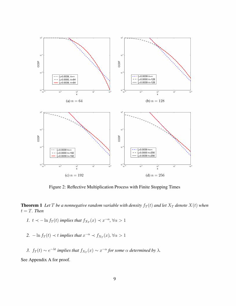
Gabaix, [17], has shown that Yn converges to an random variable with a Pareto distribution as n→ ∞.The smaller the reflection bound ξ, the slower the convergence. With finite stopping time n, thedistribution of Yn is determined by {Y0, ξ, n}. We illustrate the convergence of the distribution of Yn
by the following example: we choose Y0 = 1, ξ = 1/28, Xn = 2mn , where {mn} are i.i.d. randomvariables with probability mass function:
P (m = l) =
13
l = −112
l = 016
l = 1
Let Zn
�log2(Yn/ξ), then the evolution of Zn is
Zn+1 = max{Zn +mn+1, 0}
Its probability mass function at time n can be solved from the corresponding Markov chain and theinitial conditionZ0 = log2(Y0/ξ). As n→ ∞, Z∞ follows a geometric distribution independent of Z0,and thus Y0 and ξ. Then the distribution of Y∞ has a power law, with ξ as its smallest value. Figure 2compares CCDFs of the multiplication process with and without reflection at different stopping time:n = 64, 128, 192, 256,∞. For each stopping time n, the distribution of the multiplication processwithout reflection (ξ = 0) can be calculated as follows: let Wk
�log2(Yk), then
Wk+1 = Wk +mk+1 (8)
We can solve for the probability mass function of Wn from the Markov chain defined by (8) andW0 = log2(Y0). From those figures, we can see for finite stopping time and small reflection bound,Xn tends to have a tail similar to lognormal, even though in the limit Xn will eventually converge to apower tail.Therefore, the multiplication process for generating a lognormal distribution is fragile to a perturbationon the reflection; if ξ = 0, it produces a lognormal distribution and otherwise a Pareto distribution.
3.3.2 The mixture mechanism
We revisit the mechanism described in Section 3.2.2. We have the following result:
8
10−10 10−5 100 105 101010−15
10−10
10−5
100C
CD
F
x
ξ=0.0039, n=∞ξ=0.0000, n=64 ξ=0.0039, n=64
(a) n = 64
10−10 10−5 100 105 101010−15
10−10
10−5
100
CC
DF
x
ξ=0.0039 n=∞ξ=0.0000 n=128ξ=0.0039 n=128
(b) n = 128
10−10 10−5 100 105 101010−15
10−10
10−5
100
CC
DF
x
ξ=0.0039 n=∞ξ=0.0000 n=192ξ=0.0039 n=192
(c) n = 192
10−10 10−5 100 105 101010−15
10−10
10−5
100
CC
DF
x
ξ=0.0039 n=∞ξ=0.0000 n=256ξ=0.0039 n=256
(d) n = 256
Figure 2: Reflective Multiplication Process with Finite Stopping Times
Theorem 1 Let T be a nonnegative random variable with density fT (t) and let XT denote X(t) whent = T . Then
1. t ≺ − ln fT (t) implies that fXT(x) ≺ x−α, ∀α > 1
2. − ln fT (t) ≺ t implies that x−α ≺ fXT(x), ∀α > 1
3. fT (t) ∼ e−λt implies that fXT(x) ∼ x−α for some α determined by λ.
See Appendix A for proof.
9
Thus we observe that the distribution of X(T ) is sensitive to the tail behavior of fT (t); if it deviatesfrom an exponential decay, the power law disappears. This points to the fragility of a power law to theassumptions regarding the specific mixture.
3.3.3 Fragility of the optimization mechanism
Optimization leads to a power law. While an optimization process does lead to a power law tail witha suitably chosen objective function and under appropriate assumptions, it appears to be a fragilemechanism against the assumptions. For example, one needs to know exactly the a priori distributionmodel in order to perform the optimization procedure leading to a power law tail. Moreover these apriori distribution models often need to have infinite tails themselves. These assumptions are difficultto satisfy in an engineering system.
3.4 Difficulty of Estimating the TailThe “waist” of the lognormal distribution and the power law distribution often look very similar. Whenthe variance is large, the body of a lognormal CCDF is very close to a straight line in the log-log plot.Given a dataset of real web file sizes, we can fit most of the samples into either a lognormal model orpower law model by tuning the parameters. The dramatic difference between these two distributionslies in the tail of their CCDFs. In a log-log plot, the CCDF of a power law decays with a constantslope; the CCDF of a lognormal distribution decays with increasing slope. However in any set ofsample data, we only have a small number of samples in the extreme tail, which means it is hard todetermine which one is a better fit.To further illustrate this difficulty, suppose we have a data-set of file sizes: {Xi, i = 1, 2, · · · ,M}. As-sume all samples in the data-set are i.i.d. samples of some random variable X with CCDF G(x).We can estimate G(x) by the empirical CCDF G(x)
�1M
∑Mi=1 I(Xi > x), where I(A) is the
indicator function of set A. G(x) is an unbiased estimate of G(x) with variance V ar[G(x)] =(1 − G(x))G(x)/M . (Note: the variance of the empirical CCDF G(x) is finite at any point x aslong as X assumes a legitimate distribution, even if the variance of X itself is infinite, as for a Pareto
distribution.) When M is large, G(x) should approach a normal distribution N(G(x),√
(1−G(x))G(x)M
).The α-confidence interval for G(x) is
[
max{
0, G(x) + a
√
(1 −G(x))G(x)
M
}
, G(x) + b
√
(1 −G(x))G(x)
M
]
where∫ b
ae−x2/2dx =
√2πα and a < 0, b > 0. When we plot the confidence interval in the log-log
plot and let G(x) � 1, the width of the confidence interval is:
W ≈ log(1 +b√Mx
) − log(1 +a√Mx
)
where Mx is the expectation of the number of files with size greater than x. W keeps increasing whenMx decreases. W will blow up when MX ≤ a2.
10

103 104 105 106 107 10810−6
10−5
10−4
10−3
10−2
10−1
100
File Size
CC
DF
ParetoLognormal
(a) Model
103 104 105 106 107 108
10−5
10−4
10−3
10−2
10−1
100
File Size
CC
DF
Shadow −− ParetoSolid −− Lognormal
(b) Confidence Interval
Figure 3: Confidence Interval for Pareto and Lognormal Models
We plot the 95% confidence interval in Figure 3 for both the Pareto and the lognormal model used in[10] to fit Crovella’s web file size data-set [2]. We observe that the confidence intervals of both modelsdiverge when file sizes grow. At the extreme tail, the two confidence intervals have a large overlap,which makes it difficult to distinguish them.This suggests that one really should take into consideration the information richness when investigatingdistributional properties based on empirical data. Any inference should be made carefully in regionswhere the information is sparse. This point is echoed by Marron et al. in their papers addressingthe variability of the heavy tailed durations in Internet traffic [18, 19]. They divided the tail of thedistribution of Internet flows’ durations into three regions: “extreme tail” – the part of the tail thatis beyond the last data point (thus with no information at all in the data); “far tail” – the part of thetail where there is some data present, but not enough to reliably understand distributional properties;and finally, “moderate tail” – the part of tail where the distributional information in the data is “rich”.It provides a framework for duration distribution analysis in Internet traffic. They also observed thewobbles in the tail of the duration distribution: the tail index varies and does not stabilize. Theiranalysis in [19] generalized the theory for heavy tail durations leading to long range dependence.
3.5 Effect of tail behavior on the design and dimensioning of algorithms andprotocols on the Internet
An important factor to consider in support of our arguments is the effect that the extreme tail of a jobsize distribution has on the configuration or design of existing mechanisms on the Internet. There donot appear to be any design problems or adjustment to existing algorithms or protocols that dependupon the fact whether a (job size) distribution has infinite variance or not, whether the tail is describedby a power law or not.
11
3.5.1 Buffer dimensioning at routers
There have been numerous studies investigating the effects on the queue length of a multiplexer fed bya heavy-tailed input [20], [21], [22]. All studies show that the tail of the queue length distribution issignificantly heavier for a heavy tailed input as opposed to a light tailed or exponential tailed input. Fora finite buffer, this implies that to maintain performance guarantees in terms of drop probability buffersof significantly larger sizes would be required with a heavy tailed input as opposed to a light tailed one.However, all the studies performed assumed an open-loop transport protocol. Files, on the Internet, are(invariably) transported by TCP which is a closed-loop transport protocol. The arguments fall apartwhen we consider the closed loop case, and loss rates in fact do not depend on the tail of the flowlength (file size) distribution. This was highlighted in simulation a study [23]. TCP is configured ortuned according to fine timescale behavior, of the orders of a typical round trip time. Longer timescaleeffects, where the extreme tail of a distribution is likely to show up, are not considered at all in thedesign of TCP. Study in [24] also suggests that TCP moderates the effect of heavy tailed file sizes.Buffer dimensioning on the Internet is done typically in tune with the bandwidth-delay product of theoutput link of the router (typical values are 2-8 times bandwidth*delay). A major consideration is tolimit the amount of queueing delay for TCP flows, since the delay affects the overall throughput of afeedback based flow control protocol like TCP. Hence the buffers are kept relatively small, and thesesmall buffers then filter out the tail effects. This implies that even if we consider open-loop transportprotocols, that share the link/buffer with TCP, the tail effects of the performance are largely filteredout due to the small buffers. A recent study [25] also shows that at small time scales network trafficcan be well represented by the Poisson model.
3.5.2 The danger of extrapolation for simulation studies
Extrapolating a distribution without evidence can have serious consequences on simulation studies.For example, in [26], Gong et al. have developed the MacLaurin series of the average waiting timein GI/GI/1 queue. Assume the service time Bn can be expressed as θXn, where {Xn} is i.i.d. withE[Xn] = 1, and {Xn} are independent of θ. Also assume the inter-arrival density f(t) has a strictlyproper rational Laplace transform. Then the average waiting time can be expressed as
E[W ](θ) =∞
∑
i=0
i+1∑
k=1
1
k
f(i)∗(k−1)(0)
(i+ 2)!E[(X1 + ...+Xk)
i+2]θi+2, (9)
where f (n)∗k (0) =
∑n−1i=0 f
(i)(0)f(n−1−i)∗(k−1) (0). The distribution knowledge for the inter-arrival and ser-
vice time enter the average waiting time in different ways. While the inter-arrival density affects thewaiting time mostly through its derivatives around the origin, high moments of the service time arevery important. Long tail distributions are poor models for average waiting time, queue length andtheir variance etc. One could fit a set of web-file size data as power law (Pareto) tailed, and give thedistribution to a simulation engineer to estimate queueing delays. The simulation engineer would gen-erate service times according to the given power law tail and as a consequence, the simulation resultswill depend heavily on how long simulation is run, as the longer it runs the greater the possibility ofgenerating an unrealistically large service time. Simulations with heavy-tailed workloads have been
12

investigated in [27]. It has been shown that simulations with power law distributions are difficult toconverge to steady state and even at steady state there is often high variability.
3.6 The Effect of a Power Law Tail on TrafficIn this section we study the impact of file size distributions on the traffic correlation structure. Inparticular, we evaluate how the tail of the file size distribution affects the LRD of the resulting net-work traffic. We perform two tests, one “visual” test, similar to the one shown in [1] that strikinglyestablished the failure of Poisson modeling, and another more formal, statistical test. Because of itssimplicity, we use the M/G/∞ input process to model web traffic. An M/G/∞ input process b(t)characterizes the number of busy servers at time t of a discrete time infinite server system fed by Pois-son arrivals of rate λ and with generic service time σ distributed according to Fσ(x). One can think ofthis as modeling the arrival of web sessions according to a Poisson process where each session desiresto transfer a file of size X and is given a rate of one unit per second. The M/G/∞ input process hasbeen shown to be versatile and tractable [28]. The auto-covariance of b(t) has been established as:
Γ(h)�cov(b(t+ h), b(t)) = λ
∞∑
r=h+1
P [σ ≥ r] (10)
To obtain strict sense self-similar traffic, σ must have a power tail, i.e., Fσ(x) ∝ 1/xα. In order toevaluate the impact of the tail of Fσ(x) on the auto-correlation of b(t), we generate two M/G/∞input processes {b1(t), b2(t)} with two service time distributions: σ1 = ds1e, where random variables1 follows a Pareto distribution, with CCDF Fs1
(x) = (c/x)α, x > c, and σ2 = ds2e, where thedistribution of s2 is the mixture of a Pareto body and an exponential tail. The CCDF of s2 is
Fs2(x) =
{
(c/x)α for c < x < x0
ke−βx for x ≥ x0
where k = cαeβx0/xα0 . Then the CCDFs of {σ1, σ2} are
P [σ1 ≥ r + 1] = P [s1 > r] =
{
1 0 ≤ r ≤ bcc( c
r)α r ≥ bcc + 1
(11)
P [σ2 ≥ r + 1] = P [s2 > r] =
1 0 ≤ r ≤ bcc( c
r)α bcc + 1 ≤ r ≤ bx0c
ke−βr r ≥ bx0c + 1
(12)
The decay in the auto-covariance function for the Pareto-body and exponential tail process is given by
Γ(h) − Γ(h + 1) =
0 0 ≤ h ≤ bcc( c
h)α bcc + 1 ≤ h ≤ bx0c
he−βh h ≥ bx0c + 1
(13)
13

Thus, we see that the auto-covariance of the process decays polynomially over a finite timescale,defined exactly by the Pareto body of the file-size distribution. Now, in [29], the authors showedthat a polynomial decaying function over a finite time scale can be fitted with arbitrary accuracy by afinite mixture of exponentials (the result was for a continuous function rather than the discrete auto-covariance as in our case, but we can view the continuous function as a limiting case of the M/G/∞arrival process as the time slot t goes to 0). The wavelet estimator [30] computes the power spectraldensity of a process over a finite frequency range, governed by the length of the data and samplingfrequency. Thus, if we applied the wavelet test to a time series (traffic process) generated by a Paretobody-exponential tail distribution, it would be statistically indistinguishable from a process generatedby a pure Pareto tail distribution over a finite frequency range. This is demonstrated in the followingsimulation experiment:The auto-covariance functions of the M/G/∞ processes {b1(t), b2(t)} can be computed from (10).For this experiment, we set the arrival rate λ = 1, Pareto parameters α = 1.5, c = 5, the turning pointfor the exponential tail x0 = G−1
1 (0.001), and the rate of exponential tail β = 0.1. Figure 4 shows thetwo CCDFs in log-log scale.
100 101 102 103 104 10510−6
10−5
10−4
10−3
10−2
10−1
100
Service Time
CC
DF
ParetoPareto+Exponential
Figure 4: CCDF of the Simulated Service Time
We simulate {b1(t), b2(t)} by generating 500, 000 arrivals for each service time distribution and run-ning them through the server system. Auto-Covariances of b1(t) and b2(t) are plotted in Figure 5. InFigure 6 and 7 we show the evolution of bi(t) over different time scales. On time scale k, bi(t) isaveraged in windows of length k
bki (n ∗ k) =1
k
k∑
j=1
bi((n− 1) ∗ k + j) i = 1, 2; n = 1, 2, · · ·
We observe that the shapes of both b1(t) and b2(t) are similar on timescales from 1 to 1000, although themagnitudes decrease with the increase of timescale, which is consistent with the self-similar propertiesdescribed in Section 2, such as equation (1) . This suggests that a power tail is not necessary for visualself-similarity within a finite range. Next we perform the wavelet test to study the impact of the tail.
14

100 101 102 10310−1
100
101
102
Lag
Aut
o−co
varia
nce
TheoreticalExperimental
(a) Pareto Service Time
100 101 102 10310−3
10−2
10−1
100
101
102
Lag
Aut
o−co
varia
nce
TheoreticalExperimental
(b) Pareto+Exponential Service Time
Figure 5: Auto-Covariance of M/G/∞ Process
Energy-scale plot is an efficient tool to identify self-similarity and estimate Hurst parameter for timeseries [31]. It plots a time series’ energy {yj}, the logarithm of the variance of the wavelet coefficients,at different time scales. It has been shown in [32] that yj is a good spectral estimator of the time seriesat the frequency determined by time scale j. The confidence interval of the estimates increases as weincreases the scale, as noted in [31]. This is due to the fact that it is essentially a power spectral density(PSD) estimator, and at higher scales it is estimating low frequency components. The finiteness of thedata-length leads to increasingly inaccurate estimates of low frequency components. The linear regionin the energy-scale plot suggests self-similarity and the slope of the linear region is an estimate of theHurst parameter. Figure 8 compares the energy-scale curves of b1(t) and b2(t). As we can observe,the two plots are indistinguishable from each other up to scale (octave) 11. From Figure 8(a), betweenoctave 6 and 12, the Hurst parameter of b1(t) can be estimated as H = 1+0.616
2= 0.808. According to
[33], the H parameter of a M/G/∞ process with Pareto service time can be calculated as H = 3−α2
,where α is the Pareto parameter. We used α = 1.5 to generate b1(t). Therefore the theoretical valueof H is 0.75. Energy-scale plot gives us a good estimate for the H parameter of b1(t). At the sametime, if we look at the Energy-scale plot of b2(t) and estimate its self-similarity index between octave6 and 12, we will get a similar estimate of H = 1+0.597
2= 0.798. If we had enough data points to
only reliably estimate up to scale 12, the presence or absence of a heavy tail makes no impact onour estimate of the self-similarity index. It is the “power waist” that is the crucial factor here. Todistinguish the two processes, one would need enough data-points to obtain reliable estimates of thePSD at low frequencies where the two processes deviate.In this section, we have argued against focusing on the tails of file size distributions in order to study,model and analyze network traffic. We have demonstrated that “waist” behavior is equally, if notmore, important. In the next section, we take it a step further, and develop a Markovian model fortraffic exhibits LRD-like behavior.
15

0 0.5 1 1.5 2 2.5 3 3.5 4 4.5 5
x 105
0
5
10
15
20
25
30
35
Time
Busy
Serv
ers
(a) Timescale= 1
0 0.5 1 1.5 2 2.5 3 3.5 4 4.5 5
x 104
0
5
10
15
20
25
30
35
Time
Busy
Serv
ers
(b) Timescale= 10
0 500 1000 1500 2000 2500 3000 3500 4000 4500 50000
5
10
15
20
25
30
35
Time
Busy
Serv
ers
(c) Timescale= 100
0 50 100 150 200 250 300 350 400 450 5000
5
10
15
20
25
30
35
Time
Busy
Serv
ers
(d) Timescale= 1000
Figure 6: Sample Path of b1(t)
0 0.5 1 1.5 2 2.5 3 3.5 4 4.5 5
x 105
0
5
10
15
20
25
30
35
Time
Busy
Serv
ers
(a) Timescale= 1
0 0.5 1 1.5 2 2.5 3 3.5 4 4.5 5
x 104
0
5
10
15
20
25
30
35
Time
Busy
Serv
ers
(b) Timescale= 10
0 500 1000 1500 2000 2500 3000 3500 4000 4500 50000
5
10
15
20
25
30
35
Time
Busy
Serv
ers
(c) Timescale= 100
0 50 100 150 200 250 300 350 400 450 5000
5
10
15
20
25
30
35
Time
Busy
Serv
ers
(d) Timescale= 1000
Figure 7: Sample Path of b2(t)
16

0 2 4 6 8 10 12 14 16 180
2
4
6
8
10
12
14
16
N=3 [ (j1,j
2)= (6,12), α−est = 0.616, Q= 0.056883 ]
Octave j
yj
(a) b1(t): Pareto Service Time
0 2 4 6 8 10 12 14 16 180
2
4
6
8
10
12
14
16
N=3 [ (j1,j
2)= (6,12), α−est = 0.597, Q= 5.3279e−08 ]
Octave j
yj
(b) b2(t): Pareto+Exponential Service Time
Figure 8: Energy-Scale plot of M/G/∞ Process
4 A Markovian model for LRD trafficWe now present a model, that is Markovian in its components, and yet exhibits LRD-like correlationand spectral behavior. The model was originally proposed by us in [34]. The crucial observation indeveloping the model is that layered nature of generation of traffic has an important role in determiningthe correlation structure for individual traffic sources.
4.1 The life of a packetLet’s consider the transmission of a packet between a sender-receiver pair on a network. The packetis transmitted when a number of things simultaneously happen. Firstly, a session has to be in progressbetween a sender-receiver pair. Next, within the session the particular application (e.g., web browsing)intermittently requests/supplies data. The sender then starts sending the data, usually according toa reliable transport protocol like TCP. The release of packets to the network is decided by the flowand congestion control mechanism. Finally, if the link layer is shared, then packets are allowed onshared access medium only one at a time. For instance, if the access medium is wireless, then packettransmission is governed by the 802.11 mechanism, with intermittent transmission (if the channel isfree) and back off stages (if the channel is busy). As is evident, a number of different conditionshave to be true, largely independent of each other, for a packet to appear on the network. Not onlythat, the timescales at which the events are occurring are disparate. The transport layer timescalecorresponds to typical round trip times, that are sub-second. Application layer on-off events (e.g.,browsing, downloading, thinking) are of the order of seconds to minutes, whereas session layer eventslast from minutes to hours (e.g., user login sessions). Clearly, one should expect multiple timescalebehavior from network traffic if it was generated using this mechanism. In the following section, wedemonstrate more precisely the multiple timescale nature of the traffic.
17
1 0
1 0
1 0 1 0
1 0
1 0 1 0
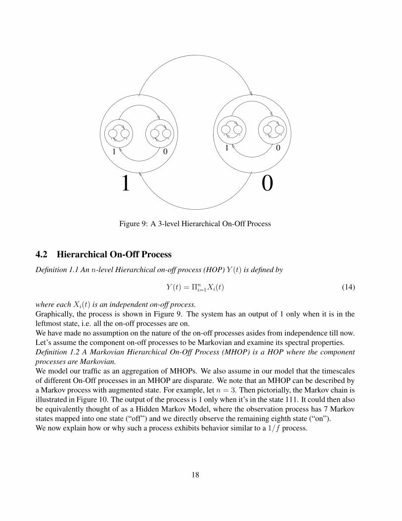
Figure 9: A 3-level Hierarchical On-Off Process
4.2 Hierarchical On-Off ProcessDefinition 1.1 An n-level Hierarchical on-off process (HOP) Y (t) is defined by
Y (t) = Πni=1Xi(t) (14)
where each Xi(t) is an independent on-off process.Graphically, the process is shown in Figure 9. The system has an output of 1 only when it is in theleftmost state, i.e. all the on-off processes are on.We have made no assumption on the nature of the on-off processes asides from independence till now.Let’s assume the component on-off processes to be Markovian and examine its spectral properties.Definition 1.2 A Markovian Hierarchical On-Off Process (MHOP) is a HOP where the componentprocesses are Markovian.We model our traffic as an aggregation of MHOPs. We also assume in our model that the timescalesof different On-Off processes in an MHOP are disparate. We note that an MHOP can be described bya Markov process with augmented state. For example, let n = 3. Then pictorially, the Markov chain isillustrated in Figure 10. The output of the process is 1 only when it’s in the state 111. It could then alsobe equivalently thought of as a Hidden Markov Model, where the observation process has 7 Markovstates mapped into one state (“off”) and we directly observe the remaining eighth state (“on”).We now explain how or why such a process exhibits behavior similar to a 1/f process.
18

&%'$
&%'$
&%'$
&%'$
&%'$
&%'$
&%'$
&%'$
PP@@
PP@@
PP@@
PP@@
PP@@
PP@@
PP@@
PP@@
`ll
`ll
`ll
`ll
`ll
`ll
`ll
`ll
`ll
`ll
`ll
`ll
JJ
JJ
""
����
011
001000
010
110
100 101
111
µ1
µ3 λ3 µ3
λ2 µ2 λ2 µ2
λ3
µ2 λ2µ2 λ2
µ1
λ1
µ1
λ1
µ1
λ1
λ1
λ3λ3 µ3 µ3
Figure 10: Markov chain representation of 3-level MHOP
4.3 Spectral Properties of the MHOPThe autocorrelation function of a Markovian on-off process is given by
Rx(τ) = pon(1 − pon)e−(λ+µ)|τ | + p2on (15)
Where λ is the transition rate from off to on and µ the rate in the reverse direction. They are relatedto pon via the relation pon = λ/(µ + λ). For the ith process, denote λi + µi by νi, p2
on by ki1 andpon(1 − pon) by ki2. The correlation of a product of two independent processes is then be just theproduct of the individual correlations, i.e.,
Rx1x2= Rx1
·Rx2
= (k11 + k12e−ν1|τ |)(k21 + k22e
−ν2|τ |)
= k11k21 + k12k21e−ν1|τ | + k11k22e
−ν2|τ | + k12k22e−(ν1+ν2)|τ |
19
The Fourier transform of the autocorrelation function gives the power spectral density, and thus wehave
Sx1x2(f) = k11k21δ(f) +
2k12k21ν1
(2πf)2 + ν21
+2k11k22ν2
(2πf)2 + ν22
+2k12k22(ν1 + ν2)
(2πf)2 + (ν1 + ν2)2
Observe the last two terms in the above expression. They can be rewritten as
(k22)(k11ν2 + k12(ν1 + ν2)) ·(2πf)2 + (ν1 + ν2)ν2ρ
((2πf)2 + ν22)((2πf)2 + (ν2 + ν1)2)
where
ρ =k11(ν2 + ν1) + k12ν2
k12(ν2 + ν1) + k11ν2
The above corresponds to the power spectral density of the response of a linear time invariant (LTI)system to white noise excitation. The LTI system has two poles at ν2 and ν1 + ν2 and a zero at√
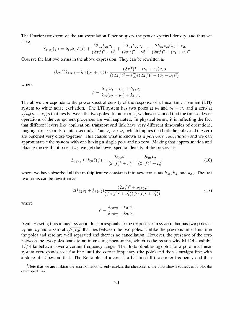
ν2(ν1 + ν2)ρ that lies between the two poles. In our model, we have assumed that the timescales ofoperations of the component processes are well separated. In physical terms, it is reflecting the factthat different layers like application, transport and link have very different timescales of operations,ranging from seconds to microseconds. Thus ν2 >> ν1, which implies that both the poles and the zeroare bunched very close together. This causes what is known as a pole-zero cancellation and we canapproximate 2 the system with one having a single pole and no zero. Making that approximation andplacing the resultant pole at ν2, we get the power spectral density of the process as
Sx1x2≈ k31δ(f) +
2k32ν1
(2πf)2 + ν21
+2k33ν2
(2πf)2 + ν22
(16)
where we have absorbed all the multiplicative constants into new constants k31, k32 and k33. The lasttwo terms can be rewritten as
2(k32ν1 + k33ν2)(2πf)2 + ν1ν2ρ
((2πf)2 + ν21)((2πf)2 + ν2
1))(17)
whereρ =
k32ν2 + k33ν1
k33ν2 + k32ν1
Again viewing it as a linear system, this corresponds to the response of a system that has two poles atν1 and ν2 and a zero at
√ν1ν2ρ that lies between the two poles. Unlike the previous time, this time
the poles and zero are well separated and there is no cancellation. However, the presence of the zerobetween the two poles leads to an interesting phenomena, which is the reason why MHOPs exhibit1/f -like behavior over a certain frequency range. The Bode (double-log) plot for a pole in a linearsystem corresponds to a flat line until the corner frequency (the pole) and then a straight line witha slope of -2 beyond that. The Bode plot of a zero is a flat line till the corner frequency and then
2Note that we are making the approximation to only explain the phenomena, the plots shown subsequently plot theexact spectrum.
20

10−2 10−1 100 101 10210−3
10−2
10−1
100
101
102
log(Frequency)
log(
Pow
er S
pect
ral D
ensi
ty)
2−level MHOP Self−Similar with H=0.88
Figure 11: Power Spectral Density for 2-level MHOP and Self-Similar Process
a straight line with slope +2 beyond that. The effect of having a zero between two poles is that therate of decay of the power spectral density slows down in the frequency region bounded on eitherside by the poles. If the zero is in exactly the middle of the two poles on the Bode plot (i.e. is thegeometric mean of the two) then the decay of the power spectral density is like that of a 1/f process,which is LRD. If the zero shifts to the left or right, then the decay is of the form 1/f γ , γ < 1 andγ > 1 respectively. This is shown in Figure 11. The two poles and the zero are marked out on theplot. We chose λ = µ for both levels and ν2 = 10ν1. Between the frequencies bounded by the twopoles, the decay of the power spectral density slows down, and goes down with a slope less than 1.A reference power spectral density of a self-similar process corresponding to a Hurst parameter of0.88 is plotted alongside. Clearly, the 2-level MHOP gives a close approximation to the self-similarprocess in the frequency range bounded by the poles. Thus, if we have an n-level MHOP, it wouldcorrespond to a cascade of such pole-zero systems and would thus tend to approximate the self-similarspectrum over the range of ν’s of all the component processes. To illustrate that, we plot a similarfigure (Figure 12) for a 3-level process, again marking out the poles and zeros and plotting a referenceself-similar process. Again, the approximation to the self-similar process over the range of ν’s (poles)is striking.The range of self-similar processes that they approximate (via the Hurst parameter), corresponds tothe range observed in network traffic [1], [31]. By changing the value of the on probability p in ourcomponent processes (thereby changing the λ/µ ratio) we can move the zero around between the polesand have considerable freedom in the range of self-similar slopes that we can approximate. Now thatwe have seen the capability of MHOPs to approximate the spectrum of self-similar processes over arange, the next natural question is that do these processes exhibit the same scaling behavior? We ran
21
10−2 10−1 100 101 10210−3
10−2
10−1
100
101
102
log(Frequency)
log(
Pow
er S
pect
ral D
ensi
ty)
3−level MHOP Self−Similar with H=0.85
Figure 12: Power Spectral Density for 3-level MHOP and Self-Similar Process
simulations and present the results in a following section.
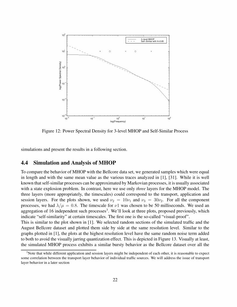
4.4 Simulation and Analysis of MHOPTo compare the behavior of MHOP with the Bellcore data set, we generated samples which were equalin length and with the same mean value as the various traces analyzed in [1], [31]. While it is wellknown that self-similar processes can be approximated by Markovian processes, it is usually associatedwith a state explosion problem. In contrast, here we use only three layers for the MHOP model. Thethree layers (more appropriately, the timescales) could correspond to the transport, application andsession layers. For the plots shown, we used ν2 = 10ν1 and ν3 = 30ν2. For all the componentprocesses, we had λ/µ = 0.8. The timescale for ν1 was chosen to be 50 milliseconds. We used anaggregation of 16 independent such processes3. We’ll look at three plots, proposed previously, whichindicate “self-similarity” at certain timescales. The first one is the so-called “visual-proof”.This is similar to the plot shown in [1]. We selected random sections of the simulated traffic and theAugust Bellcore dataset and plotted them side by side at the same resolution level. Similar to thegraphs plotted in [1], the plots at the highest resolution level have the same random noise term addedto both to avoid the visually jarring quantization effect. This is depicted in Figure 13. Visually at least,the simulated MHOP process exhibits a similar bursty behavior as the Bellcore dataset over all the
3Note that while different application and session layers might be independent of each other, it is reasonable to expectsome correlation between the transport layer behavior of individual traffic sources. We will address the issue of transportlayer behavior in a later section
22

0 100 200 3000
1000
2000
3000
4000
5000
Time Unit = 10 Seconds
Pac
kets
/Tim
e U
nit
Simulated 3−level MHOP
0 100 200 3000
1000
2000
3000
4000
5000
6000
Time Unit = 10 Seconds
Pac
kets
/Tim
e U
nit
Bellcore August Dataset
0 200 400 600 800 10000
200
400
600
800
Time Unit = 1 Second
Pac
kets
/Tim
e U
nit
0 200 400 600 800 10000
200
400
600
800
1000
Time Unit = 1 Second
Pac
kets
/Tim
e U
nit
0 200 400 600 800 10000
20
40
60
80
100
120
Time Unit = 0.1 Second
Pac
kets
/Tim
e U
nit
0 200 400 600 800 10000
20
40
60
80
100
120
Time Unit = 0.1 Second
Pac
kets
/Tim
e U
nit
0 200 400 600 800 10000
2
4
6
8
10
12
Time Unit = 0.01 Second
Pac
kets
/Tim
e U
nit
0 200 400 600 800 10000
5
10
15
Time Unit = 0.01 Second
Pac
kets
/Tim
e U
nit
Figure 13: “Visual” proof of Self-similarity
23
100 101 102 10310−1
100
101
102
log10(m)
log1
0(V
aria
nce)
Simulated 3−level MHOP Bellcore October DatasetReference Slope of −1
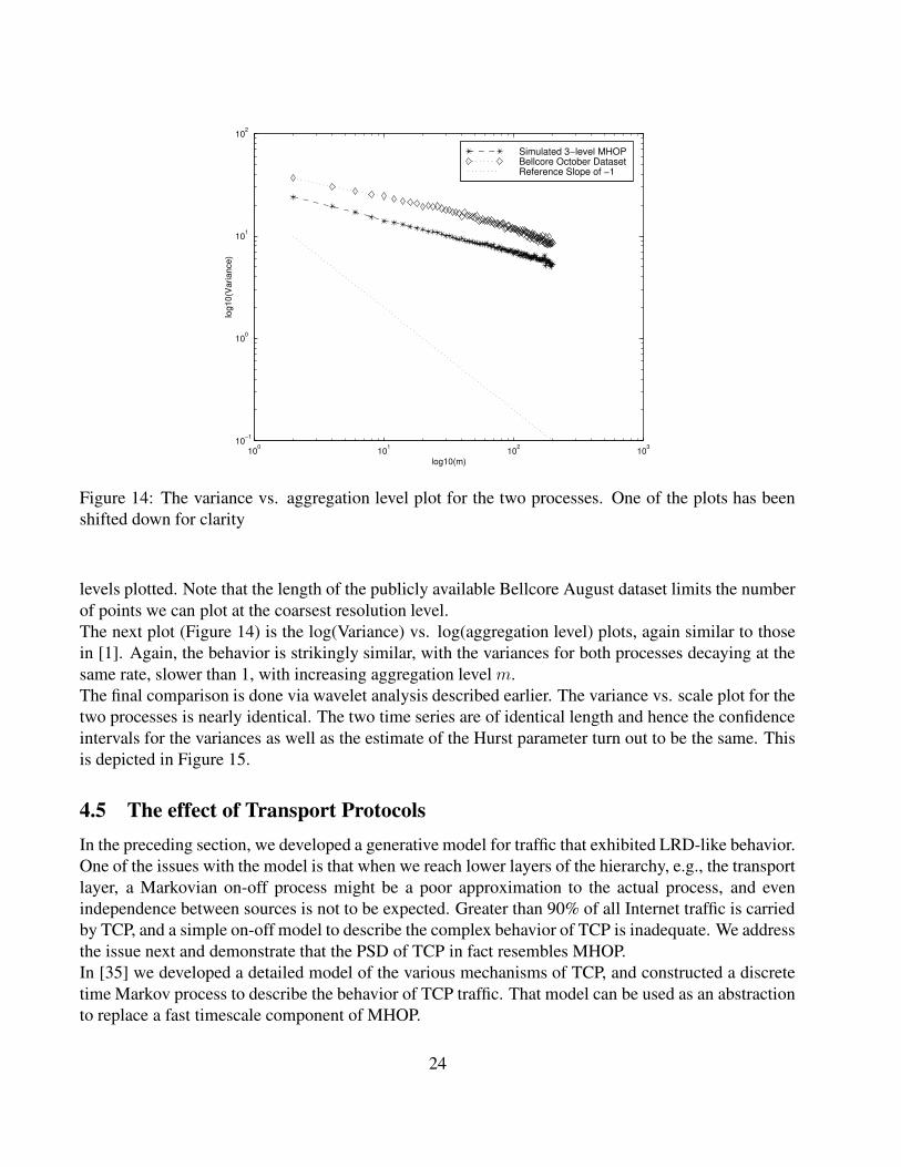
Figure 14: The variance vs. aggregation level plot for the two processes. One of the plots has beenshifted down for clarity
levels plotted. Note that the length of the publicly available Bellcore August dataset limits the numberof points we can plot at the coarsest resolution level.The next plot (Figure 14) is the log(Variance) vs. log(aggregation level) plots, again similar to thosein [1]. Again, the behavior is strikingly similar, with the variances for both processes decaying at thesame rate, slower than 1, with increasing aggregation level m.The final comparison is done via wavelet analysis described earlier. The variance vs. scale plot for thetwo processes is nearly identical. The two time series are of identical length and hence the confidenceintervals for the variances as well as the estimate of the Hurst parameter turn out to be the same. Thisis depicted in Figure 15.
4.5 The effect of Transport ProtocolsIn the preceding section, we developed a generative model for traffic that exhibited LRD-like behavior.One of the issues with the model is that when we reach lower layers of the hierarchy, e.g., the transportlayer, a Markovian on-off process might be a poor approximation to the actual process, and evenindependence between sources is not to be expected. Greater than 90% of all Internet traffic is carriedby TCP, and a simple on-off model to describe the complex behavior of TCP is inadequate. We addressthe issue next and demonstrate that the PSD of TCP in fact resembles MHOP.In [35] we developed a detailed model of the various mechanisms of TCP, and constructed a discretetime Markov process to describe the behavior of TCP traffic. That model can be used as an abstractionto replace a fast timescale component of MHOP.
24

1 2 3 4 5 6 7 8 9 10100
101
102
103
log2(scale)
log(
Var
ianc
e of
Wav
elet
Coe
ffici
ents
)
Simulated 3−level MHOP Bellcore August Dataset
Figure 15: The variance scale plot for Bellcore Dataset and Simulated Process
The power spectral density function of a discrete-time Markov process can be expressed in term of theeigenvalues of the transition probability matrix. This result was derived in [36] and is given by:
ψ(ω) =∑
l
βl(1 − λ2l )
1 − 2λl cos(ωT ) + λ2l
where ω is the frequency in radians, λl is the l-th eigenvalue of the transition probability matrix ofthe Markov chain, and βl is the average power contributed by λl as defined in [36]. The parameter Trepresents the time unit of the process, which in the model R, one round trip time.Note that each eigenvalue λl contributes a component to ψ(ω) over all frequencies. The contributionof λi is given by:
ψi(ω) =βi(1−λ2
i)
(1−λi)2+4λi sin2(ωT/2)
where the identity cos(ωT ) = 1 − 2 sin2(ωT/2) was applied.Assuming wT � 1, we have sin(ωT
2) ≈ ωT
2. As detailed in [35], this assumption is valid for frequen-
cies of interest. We then have
ψi(ω) =βi(1 − λ2
i )/λ0T2
(
1 − λi√λiT
)2
+ ω2
Observe that the form of the PSD matches what we had for MHOP, i.e. a summation of first orderterms, each term defined by an eigenvalue of the transition probability matrix. Thus, if the eigenvalues
25

are “well separated”, as in MHOP, the process exhibits LRD-like behavior following the analysisof MHOP. Details of the model and its analysis are available in [35], but essentially the value ofthe eigenvalues depends on the loss probability and round trip time experienced by TCP flows. Wereproduce a figure from the paper, that depicts the PSD of the model along with wavelet analysis ofsimulated traces of the actual TCP protocol using the ns-2 simulator. Note that the traces are for asingle long-lived flow, so there is no power law distribution involved in the generation of this traffic.We cannot over emphasize this point, that the LRD-like PSD is completely protocol determined andfile sizes are of little consequence as long as the transfer is long enough to generate data in the righttimescales.The packet rate time series was generated using the simulation packet trace with a bin size of theaverage RTT (R = 100 ms). Figure 16 shows the results of the wavelet analysis of the normalizedtime series for different loss probabilities. The solid line indicates the simulation results with a 95%confidence interval denoted by a vertical line over integer values of the time-scale. The dashed lineis the PSD of the TCP model, and the predicted time-scale marked on the plot depicts the time-scalecorresponding to the last eigenvalue of the TCP model. The time-scale is the model prediction wherethe process starts to lose its correlation structure and the PSD/wavelet energy plot is expected to flattenout.Our first observation from Figure 16 is that a single TCP flow exhibits sustained correlation over afinite range of time-scales. We note that this correlation structure is present across all loss probabilities.Note that as the loss probability increases, the time-scales over which sustained correlation structureis present increases. For a loss probability of 0.01, the time-scales range from 2R to 64R, while fora loss probability of 0.3 it ranges from 2R to 1024R, which corresponds to a range from 0.2 to 102.4seconds (almost two minutes). The wavelet plot then flattens out at higher timescales. Coupled withhigher layers of the protocol stack and utilizing the MHOP model, it is not surprising that Internettraffic exhibits LRD-like behavior regardless of the tail behavior of the distribution of the data beingtransferred.
5 ConclusionsIn this paper we have argued that the focus on power law tails in the Internet is misguided. First, manymechanisms have been proposed to explain where they come from. However, they are all very fragile,sensitive to the underlying assumptions. Second, it is extremely difficult if not impossible to statis-tically characterize a distribution tail based on a finite amount of data. Third, in many applications,the tail plays little role in determining design and performance. Instead, it is the power “waist” thatdoes. The latter was illustrated through a simple example. Multiplicative model may be the source forthe “power law” waist that has been observed. This model suggests that hierarchies and proportionalgrowth could be the mechanisms behind the multiplications in the model, and in-homogeneity of thehierarchies and the growth could be handled by appropriate clustering. One important feature of themultiplicative model is that it is similar to the central limit theorem based models where many “small”random effects add to the very robust Gaussian “body”. In our case we would say that the observedpower law or log-normal “waist” is due to many “small” random effects multiplied together. To this
26

-4
-3
-2
-1
0
1
2
3
4
5
6
0 1 2 3 4 5 6 7 8 9 10 11 12 13 14
Ene
rgy
Loss = 1%
NS trace
TCP model
��� ������� � �����������
predictedtime-scale
-4
-3
-2
-1
0
1
2
3
4
5
6
0 1 2 3 4 5 6 7 8 9 10 11 12 13 14
Ene
rgy
Loss = 5%
NS trace
TCP model
��� �������� � ������ �!�"
predictedtime-scale
-4
-3
-2
-1
0
1
2
3
4
5
6
0 1 2 3 4 5 6 7 8 9 10 11 12 13 14
Ene
rgy
Loss = 10%
NS trace
TCP model
#�$ %�&�'(�) * &�+�,�-�.�/
predictedtime-scale
-4
-3
-2
-1
0
1
2
3
4
5
6
0 1 2 3 4 5 6 7 8 9 10 11 12 13 14
Ene
rgy
Loss = 20%
NS trace
TCP model
0�1 2�3�45�6 7 3�8�9�:�;�<
predictedtime-scale
Figure 16: Wavelet analysis of simulation traces at differing loss levels and comparison with a TCPmodel
end we would also like to point out that the Gaussian distribution in engineering practice refers to itsbell, and not the tail. The latter is also for the mathematical convenience and is as unrealistic as anyother tail.In the second half of the paper, we have presented alternate models that explain the LRD-like behaviorof Internet traffic. We argue that the generation mechanism of traffic is inherently multiple timescale,and hence sustained correlations are inevitable. Coupled with that is the fact that TCP, the protocolthat carries upward of 90% of Internet traffic, generates sustained correlations on its own.Our point in this paper is that while limiting distributions of filesizes (e.g., power-law or lognor-mal tails) offer a mathematically convenient and elegant explanation for LRD, they are fraught withproblems. The effort, instead, should be on studying the complex nature of generation of traffic andunderstanding its implications.
References[1] Will E. Leland, Murad S. Taqqu, Walter Willinger, and Daniel V. Wilson, “On the self-similar
nature of ethernet traffic (extended version),” IEEE/ACM Transactions on Networking, vol. 2,no. 1, pp. 1–15, February 1994.
27

[2] M. E. Crovella and A. Bestavros, “Self-similarity in world wide web traffic: Evidence andpossible causes,” IEEE/ACM Transactions on Networking, vol. 5(6), pp. 835–846, December1997.
[3] J. M. Carlson and J. Doyle, “Highly optimized tolerance: A mechanism for power laws indesigned systems,” Physical Review E, vol. 60, pp. 1412–1427, 1999.
[4] X. Zhu, J. Yu, and J. Doyle, “Heavy tails, generalized coding, and optimal web layout,” inProceedings of IEEE/INFOCOM 01, April 2001.
[5] M. Faloutsos, P. Faloutsos, and C. Faloutsos, “On power-law relationships of the internet topol-ogy,” in Proceedings of ACM/SigComm ’99, 1999, pp. 251–262.
[6] M. Mitzenmacher, “A brief history of generative models for power law and lognormal distribu-tions,” Internet Mathematics, 2003.
[7] P. Bak, Ed., How Nature Works: the science of self-organized criticality, Springer-Verlag, 1991.
[8] W. J. Reed, “The double pareto-lognormal distribution - a new parametric model for size distri-bution,” http://www.math.uvic.ca/faculty/reed/index.html.
[9] A.L. Barabasi and R. Albert, “Emergence of scaling in random networks,” Science, vol. 286, pp.509–512, 2000.
[10] A. B. Downey, “The structural cause of file size distributions,” in Proceedings ofIEEE/MASCOTS’01, 2001.
[11] Kevin Thompson, Gregory Miller, and Rick Wilder, “Wide-area Internet traffic patterns andcharacteristics,” IEEE Network, November/December 1997.
[12] C. Fraleigh, S. Moon, B. Lyles, C. Cotton, M. Khan, D. Moll, R. Rockell, T. Seely, and C. Diot,“Packet-Level Traffic Measurements from the Sprint IP Backbone,” IEEE Network, 2003.
[13] S. Robert and J. Y. Le Boudec, “On a markov modulated chain with pseudo-long range depen-dences,” Performance Evaluation, vol. 27 – 28, pp. 159 – 173, Oct. 1996.
[14] G.W. Wornell and A.V. Oppenheim, “Estimation of fractal signals from noisy measurementsusing wavelets,” IEEE Transactions on Signal Processing, vol. 40, no. 3, pp. 611–623, Mar.1992.
[15] Jin Cao, William S. Cleveland, Dong Lin, and Don X. Sun, “Internet Traffic Tends TowardPoisson and Independent as the Load Increases,” in Nonlinear Estimation and Classification, C.Holmes, D. Denison, M. Hansen, B. Yu and B. Mallick, Ed. Springer, New York, 2002.
[16] M. Mitzenmacher, “Dynamic models for file sizes and double pareto distributions,” in preprint,2002.
28

[17] X. Gabaix, “Zipf’s law for cities: an explanation,” Quarterly Journal of Economics, August1999.
[18] F. Hernandez-Campos, J. S. Marron, G. Samorodnitsky, and F. D. Smith, “Variable heavytail duration in internet traffic, part i: Understanding heavy tails,” in Proceedings ofIEEE/MASCOTS’02, October 2002.
[19] F. Hernndez-Campos, J. S. Marron, G. Samorodnitsky, and F. D. Smith, “Variable heavy tailduration in internet traffic, part ii: Theoretical implications,” in Proceedings of 40th AllertonConference on Communication, Control and Computing, October 2002.
[20] I. Norros, “A storage model with self-similar input,” Queueing Systems, vol. 16, pp. 387–396,1994.
[21] Ashok Erramilli, Onuttom Narayan, and Walter Willinger, “Experimental queueing analysis withlong-range dependent packet traffic,” IEEE/ACM Transactions on Networking., vol. 4, no. 2, pp.209–223, 1996.
[22] P. Jelenkovic and P. Momcilovic, “Capacity regions for network multiplexers with heavy-tailedfluid on-off sources,” in Proceedings of IEEE/INFOCOM 01, April 2001.
[23] Y. Joo, V. Ribeiro, A. Feldmann, A. Gilbert, and W. Willinger, “On the impact of variability onthe buffer dynamics in IP networks,” in Allerton Conference on Communication, Control andComputing, September 1999.
[24] Kihong Park, Gitae Kim, and Mark E. Crovella, “On the effect of traffic self-similarity onnetwork performance,” in Proceedings of the SPIE International Conference on Performanceand Control of Network Systems, 1997.
[25] T. Karagiannis, M. Molle, M. Faloutsos, and A. Broido, “A nonstationary poisson view of internettraffic,” in Proceedings of IEEE/INFOCOM 2004, 2004.
[26] W.B. Gong, S. Nananukul, and A. Yan, “Pade Approximations for Stochastic Discrete EventSystems,” IEEE Transactions on Automatic Control, vol. 44, no. 12, pp. 1394–1404, August1995.
[27] Mark E. Crovella and Lester Lipsky, “Long-lasting transient conditions in simulations withheavy-tailed workloads,” in Proceedings of the 1997 Winter Simulation Conference, 1997.
[28] M. Parulekar and A. Makowski, “M/G/infinity input processes: A versatile class of models fornetwork traffic,” in Proceedings of IEEE/INFOCOM’ 97, April 1997.
[29] Anja Feldmann and Ward Whitt, “Fitting mixtures of exponentials to long-tail distributions toanalyze network performance models,” in Proceedings of IEEE/INFOCOM (3), 1997, pp. 1096–1104.
29
[30] D. Veitch and P. Abry, “Matlb code for the estimation of scaling exponents,”http://www.cubinlab.ee.mu.oz.au/∼darryl/secondorder code.html.
[31] D. Veitch and P. Arby, “A wavelet based joint estimator of the parameters of long-range depen-dence,” IEEE/ACM Transaction on Information Theory, April 1999.
[32] P. Abry, P. Goncalves, and P. Flandrin, “Wavelets, spectrum estimation, 1/f processes,” Waveletsand Statistics, Lecture Notes in Statistics, vol. 105, pp. 15–30, 1995.
[33] M. Parulekar, “Buffer engineering for M/G/Infinity input process,” Ph.D Thesis, University ofMaryland, College Park, February 2000.
[34] Vishal Misra and Wei Bo Gong, “A hierarchical model for teletraffic,” in Proceedings of the 37thAnnual IEEE CDC, 1998, pp. 1674–1679.
[35] Daniel Ratton. Figueiredo, Benyuan Liu, Vishal Misra, and Don Towsley, “On the Autocorre-lation Structure of TCP Traffic,” Computer Networks:Special Issue on ”Advances in Modelingand Engineering of Long-Range Dependent Traffic, 2001.
[36] San qi Li and Chia-Lin Hwang, “Queue response to input correlation functions: discrete spectralanalysis,” IEEE/ACM Transactions on Networking, vol. 1, no. 5, pp. 522–533, 1993.
A Proof of Theorem 1From equation (5), we have
fXt(x, t) ≺ fXt
(x, s) ≺ x−β; ∀β ≥ 0, 0 ≤ t < s (18)
and∂
∂tfXt
(x, t) =fXt
(x, t)
2σ2((ln x− lnX0)
2
t2− σ2
t− (µ− σ2/2)2)
∀T0 > 0, if (ln x − lnX0) > max{√
2σ2T0,√
2T0(µ − σ2/2)}, then ∂∂tfXt
(x, t) > 0 for t ∈ [0, T0].Thus for any distribution fT (t),
∫ T0
0
fT (t) × fXt(x, t)dt <
∫ T0
0
fT (t) × fXT0(x, T0)dt < fXT0
(x, T0) ≺ x−β ∀β ≥ 0 (19)
(1) ∀α > 1, in equation (7), we can choose λ = λ1, s.t. β1 > α− 1. Then∫ ∞
0
λ1e−λ1t × fXt
(x, t)dt =β1θ
β1 + θ(x
X0
)−β1−1 ≺ x−α
t ≺ − ln fT (t) ⇒ ∃T0, s.t. fT (t) < λ1e−λ1t, for t > T0.
∫ ∞
T0
fT (t) × fXt(x, t)dt <
∫ ∞
0
λ1e−λ1t × fXt
(x, t)dt ≺ x−α (20)
30
From (19) and (20), we have
fXT(x) =
∫ T0
0
fT (t) × fXt(x, t)dt+
∫ ∞
T0
fT (t) × fXt(x, t)dt ≺ x−α
(2) ∀α > 1, in equation (7), we can choose λ = λ2, s.t. β2 < α− 1. Thus
x−α ≺∫ ∞
0
λ2e−λ2t × fXt
(x, t)dt =β2θ
β2 + θ(x
X0)−β2−1 (21)
− ln fT (t) ≺ t⇒ ∃T0, s.t. fT (t) > λ2e−λ2t, for t > T0.
From equation (19),∫ T0
0
λ2e−λ2t × fXt
(x, t)dt ≺ x−α
together with (21)
x−α ≺∫ ∞
T0
λ2e−λ2t × fXt
(x, t)dt
Finally,
fXT(x) >
∫ ∞
T0
fT (t) × fXt(x, t)dt >
∫ ∞
T0
λ2e−λ2t × fXt
(x, t)dt
Therefore, x−α ≺ fXT(x)
(3) From equation (6),∫ ∞
0
c1e−λt × fXt
(x)dt = c2x−α (22)
Given limt→∞fT (t)
c1e−λt = 1, ∀ε > 0, ∃T (ε) s.t. if t ≥ T (ε),
(1 − ε)c1e−λt ≤ fT (t) ≤ (1 + ε)c1e
−λt (23)
From (19),∫ T (ε)
0fT (t) × fXt
(x)dt ≺ x−α, therefore ∃X1(ε), s.t. for x > X1(ε),
∣
∣
∣
∣
∫ T (ε)
0
fT (t) × fXt(x)dt
∣
∣
∣
∣
≤ εx−α (24)
Likewise,∫ T (ε)
0c1e
−λt × fXt(x)dt ≺ x−α, ∃X2(ε), s.t. for x > X2(ε),
∣
∣
∣
∣
∫ T (ε)
0
c1e−λt × fXt
(x)dt
∣
∣
∣
∣
≤ εx−α (25)
31
Let X(ε) = max{X1(ε), X2(ε)}, for x > X(ε),∣
∣
∣
∣
∫ ∞0fT (t) × fXt
(x)dt
x−α− c2
∣
∣
∣
∣
≤∣
∣
∣
∣
∫ ∞T (ε)
fT (t) × fXt(x)dt
x−α− c2
∣
∣
∣
∣
+
∣
∣
∣
∣
∫ T (ε)
0fT (t) × fXt
(x)dt
x−α
∣
∣
∣
∣
≤∣
∣
∣
∣
∫ ∞T (ε)
c1e−λt × fXt
(x)dt
x−α− c2
∣
∣
∣
∣
+ε×∣
∣
∣
∣
∫ ∞T (ε)
c1e−λt × fXt
(x)dt
x−α
∣
∣
∣
∣
+ε by (23) and (24)
≤∣
∣
∣
∣
∫ T (ε)
0c1e
−λt × fXt(x)dt
x−α
∣
∣
∣
∣
+ε× c2 + ε by (22)
≤ε× (c2 + 2) by (25)
In other words, ∀ε > 0, ∃X(ε), s.t. for x > X(ε),∣
∣
∣
∣
∫ ∞0fT (t) × fXt
(x)dt
x−α− c2
∣
∣
∣
∣
≤ ε× (c2 + 2),
so we have
limx→∞
∫ ∞0fT (t) × fXt
(x)dt
x−α= c2
32